Effects of Climatic Disturbance on the Trade-Off between the Vegetation Pattern and Water Balance Based on a Novel Model and Accurately Remotely Sensed Data in a Semiarid Basin

Abstract

Vegetation is a natural link between the atmosphere, soil, and water, and it significantly influences hydrological processes in the context of climate change. Under global warming, vegetation greening significantly aggravates the water conflicts between vegetation water use and water resources in water bodies in arid and semiarid regions. This study established an improved eco-hydrological coupled model with related accurately remotely sensed hydrological data (precipitation and soil moisture levels taken every 3 j with multiply verification) on a large spatio-temporal scale to determine the optimal vegetation coverage (M*), which explored the trade-off relationship between the water supply, based on hydrological balance processes, and the water demand, based on vegetation transpiration under the impact of climate change, in a semiarid basin. Results showed that the average annual actual vegetation coverage (M) in the Hailar River Basin from 1982 to 2012 was 0.62, and that the average optimal vegetation coverage (M*) was 0.56. In 67.23% of the region, M* was lower than M, which aggravated the water stress problem in the Hailar River Basin. By identifying the sensitivity of M* to vegetation characteristics and meteorological parameters, relevant suggestions for vegetation-type planting were proposed. Additionally, we also analyzed the dynamic threshold of vegetation under different climatic conditions, and we found that M was lower than M* under only four of the twenty-eight climatic conditions considered (rainfall increase by 10%, 20%, and 30% with no change in temperature, and rainfall increase by 20% with a temperature increase of 1 °C), thereby meeting the system equilibrium state under the condition of sustainable development. This study revealed the dynamic relationship between vegetation and hydrological processes under the effects of climate change and provided reliable recommendations to support vegetation management and ecological restoration in river basins. The remote sensing data help us to extend the model in a semiarid basin due to its accuracy.

1. Introduction

Vegetation, as an important ecosystem component, plays a vital role in maintaining the hydrological balance between watersheds and their response to climate change [1]. Climate change is a key influencing factor of vegetation that can affect hydrological processes through a range of biophysical processes [2,3,4]. Vegetation and hydrological processes have a mutually interactive relationship, whereby vegetation can influence hydrological processes in a watershed by affecting rainfall, and hydrological processes can affect vegetation growth through factors such as soil water storage [5,6]. Therefore, recognizing the interactions between vegetation and hydrological processes is important for maintaining the ecological balance of watersheds in the context of global climate change.

Vegetation coverage is a reflection of the ecological robustness of a watershed and its capacity to change [7,8]. Over the past three decades, the normalized difference vegetation index (NDVI) has shown an increasing trend in most regions of China, including some arid and semiarid regions [9,10]. Even though vegetation in China accounts for only 6.6% of the global total, studies have shown that China has contributed 25% of the global net increase in green foliage during 2000–2017 [11]. Vegetation reduces water availability through evapotranspiration, but it can also increase the regional water availability by enhancing the soil permeability and water-holding capacity [12,13]. Thus, ecosystem evapotranspiration can increase with vegetation greening, which can accelerate atmospheric water recirculation and increase precipitation under certain circumstances [14]. Similarly, through net hydrological impacts, vegetation greening can increase regional water availability [15,16]. Studies have shown that vegetation greening in humid areas has not substantially reduced runoff and soil moisture in watersheds by enhancing water recirculation, whereas this has not been the case in arid areas [17]. In arid regions, vegetation greening might lead to a series of negative ecohydrological effects in watersheds, such as reduced river runoff, insufficient ecological water demand, soil salinization, and reduced species diversity [18,19]. Wu et al. [20] found that the main cause of runoff attenuation in the transition zone between the Qinling Mountains and the Loess Plateau was vegetation greening. In water-limited regions, changes in evapotranspiration and runoff due to vegetation greening are notably larger than in energy-limited regions; thus, the phenomenon of vegetation greening in arid zones can exacerbate water scarcity [21,22].

Eagleson suggested that vegetation can reach optimal coverage during long-term environmental adaptation, beyond which, watersheds are at risk of ecological disequilibrium. When compared to both statistical models that cannot determine the mutual mechanisms between vegetation and climate factors and vegetation models that are time-consuming and require large numbers of parameters in operation, Eagleson’s ecohydrological model is simple and has a physical mechanism that describes the equilibrium relationship between soil, vegetation, and climate [23,24]. This model indicates that the state of vegetation—whether it achieves an equilibrium relationship with local hydroclimatic conditions—significantly influences the water budget. At arid and semiarid regions, precipitation variation and associated soil moisture dynamics are quite different and are involved in pulsing characteristics. This situation required long-term, large-scale, highly accurate surface data. However, there is lack of validation in terms of the applicability of the model in arid and semiarid regions. For example, the key hydrological elements, such as precipitation and soil moisture, governed the hydrological balance one day sooner than the required time scale for related high-quality remotely sensed data and validation [25,26]. Moreover, previous studies reported problems in using the model to simulate runoff when the average ecohydrological balance of a watershed was simulated [27,28]. The Budyko framework, which is based on water balance mechanisms, climate change, and vegetation dynamics, has been used widely in runoff prediction because of its simplicity [29,30]. However, few studies have extended the application range of the Budyko-type model to other ecohydrological model [31,32].

In semiarid and arid regions, there is a persistent trade-off between plant growth and water consumption. On the one hand, enhanced vegetation cover provides numerous ecological benefits, including soil erosion control and increased carbon sequestration [23,25,31]. On the other hand, the expansion of vegetation cover results in higher water consumption through the process of transpiration. Recognizing the trade-off or dynamic equilibrium between vegetation dynamics and hydrological processes under the impact of climate change, especially for arid and semiarid regions with precipitation constraints, is important in facilitating the management of watershed ecosystems and maintaining optimal ecosystem function [33,34]. Here, we selected the Hailar River Basin in the Inner Mongolia Autonomous Region of China as the study area. This region comprises an organic combination of large grassland and forest ecosystems that provide rich vegetation resources and constitute an important ecological security barrier in northern China; it is also a typical semiarid region [35,36,37]. On the basis of an improved ecohydrological model, our study explored the trade-off relationship between water supply, based on hydrological balance processes, and water demand, based on vegetation transpiration under climate change, in the Hailar River Basin. Our specific objectives were as follows: (1) to propose an improved ecohydrological model to depict the climate, vegetation, and hydrological processes, which is more applicable to arid and semiarid regions; (2) to validate the long-term, large-scale, highly accurate surface soil moisture (remote sensed related data) using multiply ground-based observation data; (3) to quantify the optimal vegetation coverage and analyze the sensitivity of the optimal vegetation coverage to vegetation parameters and meteorological parameters; and (4) to discuss how the optimal vegetation coverage and the actual vegetation coverage vary under different climatic conditions.

2. Materials and Methods

2.1. Study Area

The study area comprised the upstream–midstream region of the Hailar River Basin (47°24′7″–50°33′8″N, 117°33′12″–122°31′4″E), which covers a total area of 43,345 km². According to meteorological data from 1979 to 2018, the annual mean precipitation and annual mean temperature of the basin are approximately 347 mm and −1.2 °C, respectively, indicating that it is a semiarid basin. The water-limited and semiarid condition of the basin raises the risk of the destruction of the ecohydrological balance. The vegetation types in the basin show marked zonal distribution from the east to the west, with deciduous broadleaved forests and montane coniferous forests primarily in the eastern region, forest–grassland transition zones in the central region, and vast grasslands in the western region. The main soil types in the basin are black, dark brown, Chernozem, and meadow soils. The study area was divided into six subwatersheds as follows: subwatersheds A, B, E, and F are dominated by forests, and subwatersheds C and D are dominated by grassland (Figure 1). Under the background of climate warming, vegetation exhibits a significant greening trend, further exacerbating water deficits in the watershed. This has led to noticeable vegetation degradation and land desertification in downstream areas. The methods to address these issues are highly consistent with the objectives of this project; hence, the study will focus on the middle and upper reaches of the Hailar River Basin.

2.2. Data Collection

2.2.1. Field Sampling Data

In this study, field sampling soil moisture (s₀) data (1 August 2016–31 July 2017) within the Hailar basin was determined through field sampling and subsequent oven-drying experiments conducted in the laboratory (Figure 1). Soil samples were collected from five different depths as follows: 0–5 cm, 5–20 cm, 20–40 cm, 40–60 cm, and 60–80 cm. These samples were initially measured in the field before being transported to the laboratory, where they were oven-dried at 105 °C.

2.2.2. In Situ Observation Data

The daily average temperature, daily maximum temperature, daily minimum temperature, sunshine duration, relative humidity, and wind speed data from 1 January 1982 to 31 December 2012 measured within the study area were collected from the China Meteorological Data Sharing Network (www.data.cma.cn, accessed on 10 May 2024). These meteorological variables were interpolated onto a 10 × 10 km grid using the inverse distance weighting method to analyze the spatial climate change characteristics within the basin. Long-term soil moisture (s₀) observation data were from the Hailar eddy-covariance flux tower (120°6′8.63″E, 49°21′10.52″N, 1 August 2016~31 December 2016), and s₀ was obtained from three depths (0–5, 5–10, and 10–20 cm) and was used simultaneously with above-field sampling data to calibrate and verify remotely sensed data. Runoff (Q) observations over the period 1982–2012 in 6 sub-catchments across were provided by the Hulunbuir Hydrological Bureau.

2.2.3. Related Remotely Sensed Data

Vegetation Data

The biweekly vegetation data indicated by the NDVI was obtained from the Global Inventory Modeling and Mapping Studies 8-day and 8 km 3g.v1 dataset from 1982 to 2012. The vegetation coverage was calculated from the NDVI data using the following equation:

$$\mathrm{M}=\frac{\mathrm{N}\mathrm{D}\mathrm{V}\mathrm{I}-{\mathrm{N}\mathrm{D}\mathrm{V}\mathrm{I}}_{\mathrm{m}\mathrm{i}\mathrm{n}}}{{\mathrm{N}\mathrm{D}\mathrm{V}\mathrm{I}}_{\mathrm{m}\mathrm{a}\mathrm{x}}-{\mathrm{N}\mathrm{D}\mathrm{V}\mathrm{I}}_{\mathrm{m}\mathrm{i}\mathrm{n}}},$$

(1)

where M is vegetation coverage, and ${\mathrm{N}\mathrm{D}\mathrm{V}\mathrm{I}}_{\mathrm{m}\mathrm{i}\mathrm{n}}$ and ${\mathrm{N}\mathrm{D}\mathrm{V}\mathrm{I}}_{\mathrm{m}\mathrm{a}\mathrm{x}}$ are the NDVI of the barren soil and forest, respectively.

Soil Moisture Data

The spatial soil moisture data used were from the Global Land Data Assimilation System Version 2 (GLDAS-2.1). The GLDAS is executed globally at a high resolution (0.25° to 1°) and can produce results in near-real time. The Global Land Data Assimilation System (GLDAS) operates on a global scale at high resolutions ranging from 0.25° to 1°. It is capable of producing near-real-time results. The GLDAS dataset provides soil moisture information for four layers as follows: 0–10 cm, 10–40 cm, 40–100 cm (https://search.earthdata.nasa.gov, accesed on 10 May 2024). The data has a spatial resolution of 0.25° and a temporal resolution of 3 h.

Precipitation Data

The precipitation data taken every three hours from 1982–2012 were provided by the China Meteorological Forcing Dataset (CMFD). The data were produced by merging TRMM satellite precipitation analysis data (3B42), GLDAS precipitation, and ground data. A single event was determined by a precipitation intensity of more than 0.1 mm d⁻¹ within 6 h. The precipitation interval and duration has also been defined by the single event.

2.3. Soil Moisture Validation

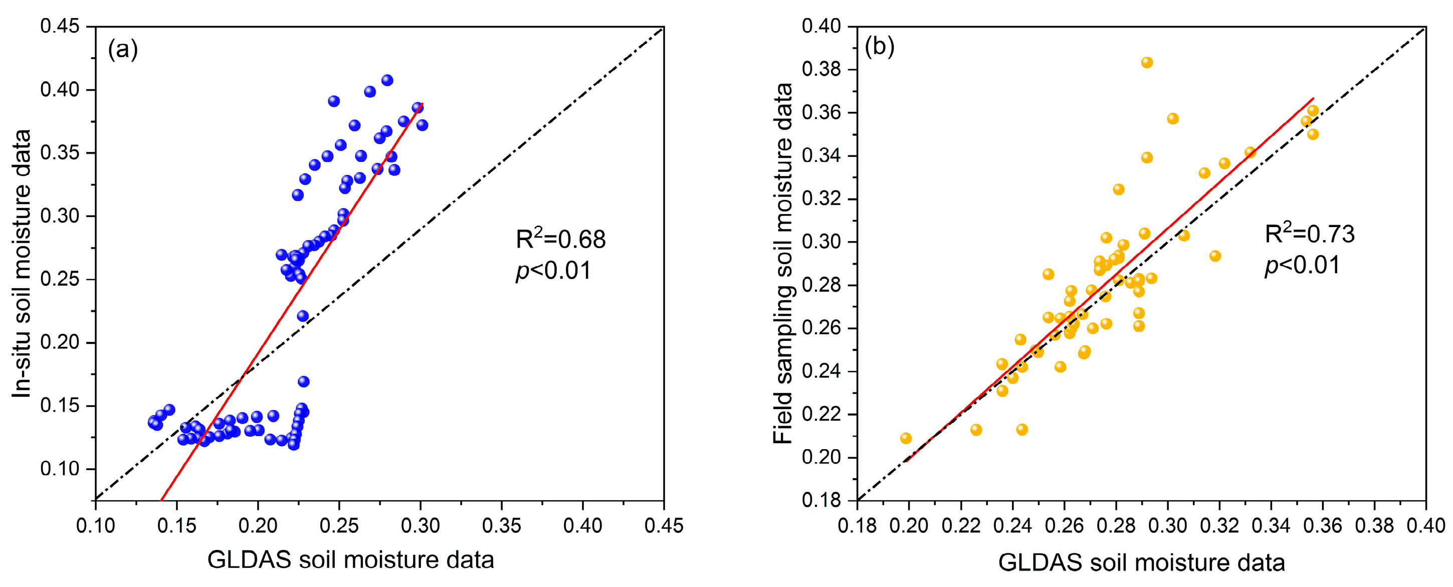
To validate the soil moisture from GLDAS data, the in situ soil moisture data from the eddy-covariance flux tower and field sampling data were used to evaluate the applicability of the GLDAS data. The results (Figure 2) showed that the coefficients of determination (R²) between the GLDAS data and in situ or field sampling data were 0.68 (p < 0.01) and 0.73 (p < 0.01), respectively. The results indicated the high performance of the soil moisture from GLDAS data in the study area.

2.4. Coupled Ecohydrological Model

2.4.1. Eagleson’s Ecohydrological Model

Eagleson’s ecohydrological model is a growing season water balance model constructed on a vertical one-dimensional scale, based on regional climate, soil, and vegetation conditions. The equation can be expressed as follows:

$$\underset{a}{\underbrace{M{k}_v^{*}{\beta }_v{m}_{tb}^{\prime }{E}_{ps}}}=m_h-\underset{b}{\underbrace{\overline{h_0}}}-\underset{c}{\underbrace{\frac{\Delta S}{m_v}}}-\underset{d}{\underbrace{m_{tb}^{″}{E}_{ps}(1-M){\beta }_s}}-\underset{e}{\underbrace{m_h{e}^{-G-2{\sigma }^{3/2}}}}-\underset{f}{\underbrace{\frac{m_t{m}_{h}K(1)}{P_{\tau }}{s}_0^c}}+\underset{g}{\underbrace{\frac{m_t{m}_{h}K(1)}{P_{\tau }}\left[1+\frac{3/2}{mc-1}\right]{\left[\frac{\psi (1)}{z_w}\right]}^{mc}}}.$$

(2)

where the terms (a)–(g) represent vegetation evapotranspiration, surface interception, soil moisture storage, bare soil evaporation, surface runoff, deep percolation, and capillary rise, respectively. The detailed algorithms of terms have been introduced in previous research [25].

In arid and semiarid regions, the proportion of deep percolation and capillary rise as a percentage of the mean storm depth is small; therefore, the term g in Equation (1) can be ignored. However, in arid and semiarid regions, the energy is limited by the potential evapotranspiration of the watershed. The vegetation coverage in these regions is small, and the competition mechanism between the soil evaporation and vegetation transpiration cannot be neglected; therefore, bare soil evaporation cannot be ignored.

2.4.2. Budyko Framework

The Budyko framework, which is based on water balance, climate change, and vegetation dynamics, has been widely used due to its simplicity and precision. The runoff simulation in the model is calculated according to the principle of hypertonic flow production; therefore, the runoff volume change with time cannot be better restored when applying the original runoff term $m_h{e}^{G-2\sigma 3/2}$ of the simulation model. Therefore, in this study, we introduced the Budyko-type model based on monthly scales in order to calculate the runoff [29] as follows:

$$\frac{ET}{P}=\frac{1+E_{ps}/P-\sqrt{(1+E_{ps}/P{)}^2-4\epsilon (2-\epsilon )E_{ps}/P}}{2\epsilon (2-\epsilon )}$$

(3)

$$\frac{R}{P}=1-\frac{ET}{P}$$

(4)

On the basis of the above improvements, we proposed a growing season water balance model based on Eagleson’s model and the Budyko framework that is more applicable to arid and semiarid regions as follows:

$$\underset{a}{\underbrace{{\mathrm{Mk}}_v^{*}{\beta }_v{m}_{tb}^{\prime }{E}_{ps}}}=m_h-\underset{b}{\underbrace{\overline{h_0}}}-\underset{c}{\underbrace{\frac{\Delta S}{m_v}}}-\underset{d}{\underbrace{m_{tb}^{″}{E}_{ps}(1-M){\beta }_s}}-\underset{e}{\underbrace{\frac{R}{m_v}}}$$

(5)

In this study, the growing season was defined as the period from the first rainfall in April to the last rainfall in September. The climate, soil, and vegetation data used as the model input that appear in the above equations and the meaning of their corresponding symbols are listed in

Table 1. Main inputs of the ecohydrological model.

Main Inputs	Name	Description	Unit
Climate conditions	md	Length of the growing season	day
	mv	Amount of precipitation	dimensionless
	mh	Rainfall event depth	mm
	mtb	Mean time between precipitation	day
	mtb′	Mean time spent on transpiration between precipitation	day
	mtb″	Mean time spent on evaporation of bare soil between precipitation	day
	Pd	Precipitation in the non-growing season	mm
	$\epsilon$	The ratio between initial and total evapotranspiration	dimensionless
Soil properties	βv	Canopy transpiration efficiency	dimensionless
	Epsd	Potential evapotranspiration during the growing season	mm day−1
	Eps	Potential evapotranspiration of moist soil	mm day−1
	βs	Evaporation efficiency of bare soil	dimensionless
Vegetation parameters	M	Average vegetation cover of the growing season	dimensionless
	Md	Average vegetation coverage of the non-growing season	dimensionless
	$k_v^{\mathrm{*}}$	Potential canopy conduction	dimensionless
	$\overline{h_0}$	Canopy precipitation interception	mm
	${\eta }_0$	The ratio of the stomal area to the leaf area	dimensionless
	Lt	Leaf area index	dimensionless
	β	Cosine of the angle the leaf surface makes with the horizon	dimensionless

.

When the vegetation transpiration coefficient ${\beta }_v$ is equal to 1, the vegetation coverage can be obtained using the following equation:

$$M{k}_v^{*}=\frac{V_{\mathrm{e}}}{m_{tb}^{\prime }{E}_{ps}}$$

(6)

where $s_0$ is the soil moisture, which can be calculated as follows:

$$s_0=m_h-\overline{h_0}-\frac{\Delta S}{m_v}-m^{″}{E}_{ps}(1-M){\beta }_s-\frac{P[2\epsilon (2-\epsilon )-1-E_{ps}/P+\sqrt{(1+E_{ps}/P{)}^2-4\epsilon (2-\epsilon )E_{ps}/P}]}{m_{v}2\epsilon (2-\epsilon )}$$

(7)

Using this model, we calculated the optimal vegetation coverage for the watershed under multiyear ecohydrological equilibrium conditions from 1982 to 2012.

3. Results

3.1. Runoff Simulation Accuracy

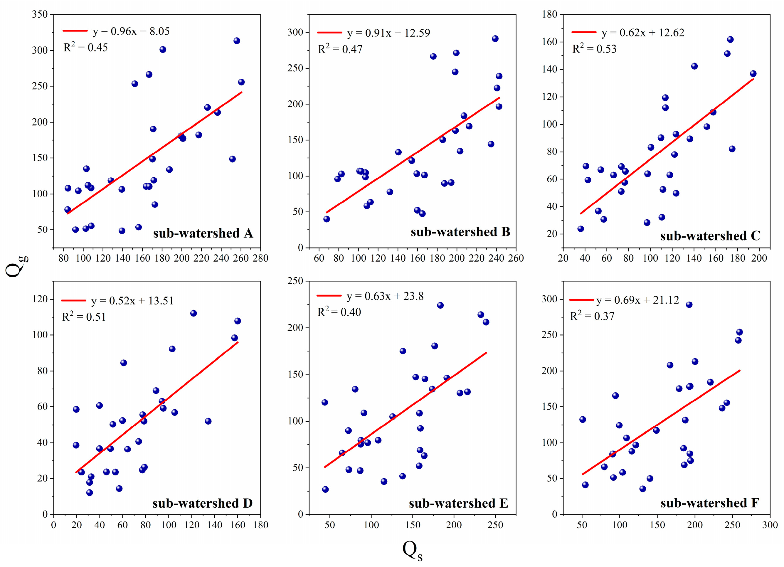
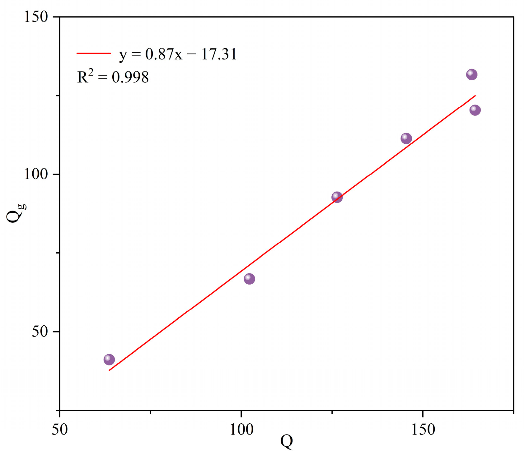
The model was validated using observed growing season runoff data from six subwatersheds, and the validation results are shown in Figure 3, where Q_s is the flow obtained from the simulation and Q_g is the measured flow during the growing season. Among the six subwatersheds, the growing season runoff from 1982 to 2012 simulated with the improved model fitted well with the measured growing season runoff, with the R² value varying from 0.37 to 0.53. In subwatersheds with a larger area, the fit was better, and the fit for subwatersheds C and D was better when compared to that for the other smaller subwatersheds. When compared to our previous studies [23,38], the simulation accuracy of the runoff term in our model was improved. Figure 4 shows that the multiyear average growing season runoff from 1982 to 2012 was generally consistent with the fit to the measured growing season runoff (R² = 0.99), which we used as the input for the runoff term in the coupled ecohydrological model.

3.2. Spatial Pattern of Multiyear M, M*, and ΔM

In this study, we compared the multiyear average (1982–2021) of the actual vegetation coverage (M) based on remote sensing with the optimal vegetation coverage (M*) based on ecological optimization theory simulation, and found no correlation between them. Additionally, we calculated ∆M (∆M = M − M*) to observe more directly the difference between the actual vegetation coverage and the optimal vegetation coverage.

The actual vegetation coverage of the watershed varied from 0.34 to 0.82, with a multiyear average actual vegetation coverage of 0.62, with the value increasing gradually from the west to the east. This is consistent with the variation in vegetation types in the watershed, i.e., grassland in the west with a low vegetation coverage and forest in the east with a high vegetation coverage. Similarly, the six subwatersheds showed statistically significant differences in the actual vegetation coverage related to the dominant vegetation type of the watershed. Subwatershed A (0.75), subwatershed B (0.72), subwatershed E (0.67), and subwatershed F (0.71) had higher multiyear average actual vegetation coverage when compared to that of subwatershed C (0.62) and subwatershed D (0.57).

The optimal vegetation coverage of the watersheds varied from 0.17 to 0.92, with a mean value of 0.56. Unlike the actual vegetation coverage, the optimal vegetation coverage did not present a clear spatial distribution, and the values of the optimal vegetation coverage did not differ much, even in areas with different major vegetation types. The values of the optimal vegetation coverage in each subwatershed were relatively close to each other, i.e., 0.48, 0.56, 0.56, 0.55, 0.56, and 0.58 for subwatersheds A–F, respectively.

Notably, the optimal vegetation coverage of each subwatershed was lower than its actual vegetation coverage; therefore, the water stress of the watershed must be considered. On the basis of the ∆M values, it was found that 67.23% of areas had optimal vegetation coverage that was lower than the actual vegetation coverage, with values varying between −0.65 and −0.01. Areas where the optimal vegetation coverage of the watershed was lower than the actual vegetation coverage are mainly located in the eastern part of the watershed in mountainous forested areas, namely subwatersheds A (−0.26), B (−0.16), E (−0.11), and F (−0.13), whereas the areas where the optimal vegetation coverage of the watershed was greater than the actual vegetation coverage are mainly located in the southwestern steppe zone, namely subwatersheds C (−0.07) and D (−0.02). Subwatershed A had the greatest actual vegetation coverage in the entire watershed, but the optimal vegetation coverage was notably smaller than that of the other areas, indicating that subwatershed A had the most severe water stress problems. The area encompassed by the blue circle in Figure 5 is the Huihe Forest, where M (0.82) is much larger than M* (0.17). This region is in the forest–grass transition area, which is relatively arid. Owing to recent ecological restoration projects, water consumption in this region has been increasing and water supply/demand problems have become serious. The blue circle is the location of planation forests in Hui River, which exhibited a large difference between M and M*. The results are likely because of the excessive afforestation in the area during recent years.

3.3. Sensitivity of M* to Vegetation Parameters

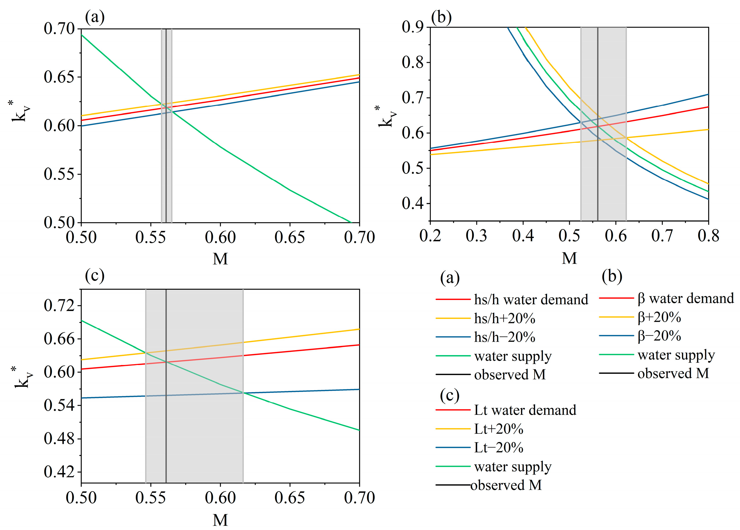
The value of M* changes with vegetation parameters, which include the cosine of the angle that the leaf surface makes with the horizon ($\beta$), the foliage area index ($L_t$), and the ratio of the height of the trunk to the height of the individual plant ($h_s/h$) (Figure 6). When $h_s/h$ increases (decreases) by 20%, the water demand curve shifts upward (downward), resulting in a decrease (increase) in M* by 0.61% (0.72%). Notably, an increase or decrease in $h_s/h$ will not change the water supply curve. However, changes to parameter $\beta$ result in changes to both the water supply curve and the water demand curve. When $\beta$ decreases by 20%, the water supply curve shifts downward, the water demand curve shifts upward, and M* decreases by 6.41%. Conversely, M* increases by 10.92% when $\beta$ increases by 20%. Moreover, when $\beta$ increases, the water supply curve shifts upward and the water demand curve shifts downward. Moreover, M* changes considerably with changes in $L_t$, especially when $L_t$ decreases. When $L_t$ increases by 20%, the water demand curve shifts upward and M* decreases by 2.51%; when $L_t$ decreases by 20%, the water demand curve shifts downward and M* increases by 9.82%. It is noted that M* is the least sensitive to $h_s/h$, and is most sensitive to increases in $\beta$ and decreases in $L_t$ (

Table 2. Sensitivity of the optimal vegetation coverage to vegetation parameters.

Vegetation Parameters	M* Change in Value		The Sensitivity of M* to Parameter Changes
	20%	−20%	20%	−20%
$h_s/h$	0.56	0.57	−0.61%	0.72%
$\beta$	0.62	0.52	10.92%	−6.41%
$L_t$	0.54	0.61	−2.51%	9.82%

).

3.4. Sensitivity of M* to Meteorological Parameters

The value of M* varies with several meteorological parameters, including the rainfall event depth ($m_h$), mean time between precipitation ($m_{tb}$), potential evapotranspiration of wet soil ($E_{ps}$), and temperature (T) (Figure 7). Overall, M* is most sensitive to $m_h$, with which it exhibits a positive correlation. When $m_h$ increases (decreases) by 20%, M* increases (decreases) by 35.56% (41.17%). Furthermore, as $m_h$ increases (decreases), the water supply curve shifts upward (downward). However, the water demand curve remains unchanged regardless of variations in $m_h$. Characteristically, M* is negatively correlated with $E_{ps}$; when $E_{ps}$ increases (decreases) by 20%, M* decreases (increases) by 14.11% (20.35%). When $E_{ps}$ increases and decreases, the water supply curve shifts downward and upward, respectively, whereas the water demand curve remains unchanged. Additionally, M* is also negatively correlated with $m_{tb}$. When $m_{tb}$ increases (decreases) by 20%, the water supply curve shifts downward (upward), resulting in a decrease (increase) in M* of 14.32% (20.12%). Changes in $m_h$, $m_{tb}$, and $E_{ps}$ lead to changes in the water supply curve, whereas changes in T lead to changes in the water supply and water demand curves. When T increases by 20%, the water supply curve shifts downward and the water demand curve shifts upward, resulting in a decrease in M* of 10.72%. In contrast, when T decreases by 20%, M* increases by 8.70%. It is noted that M* is the least sensitive to T (

Table 3. Sensitivity of the optimal vegetation coverage to meteorological parameters.

Meteorological Parameters	M* Change in Value		The Sensitivity of M* to Parameter Changes
	20%	−20%	20%	−20%
$m_h$	0.76	0.33	35.56%	−41.17%
$m_{tb}$	0.48	0.67	−14.32%	20.12%
$E_{ps}$	0.48	0.67	−14.11%	20.35%
T	0.50	0.60	−10.72%	8.70%

).

3.5. Analysis of Vegetation Coverage Threshold under Different Climate Conditions

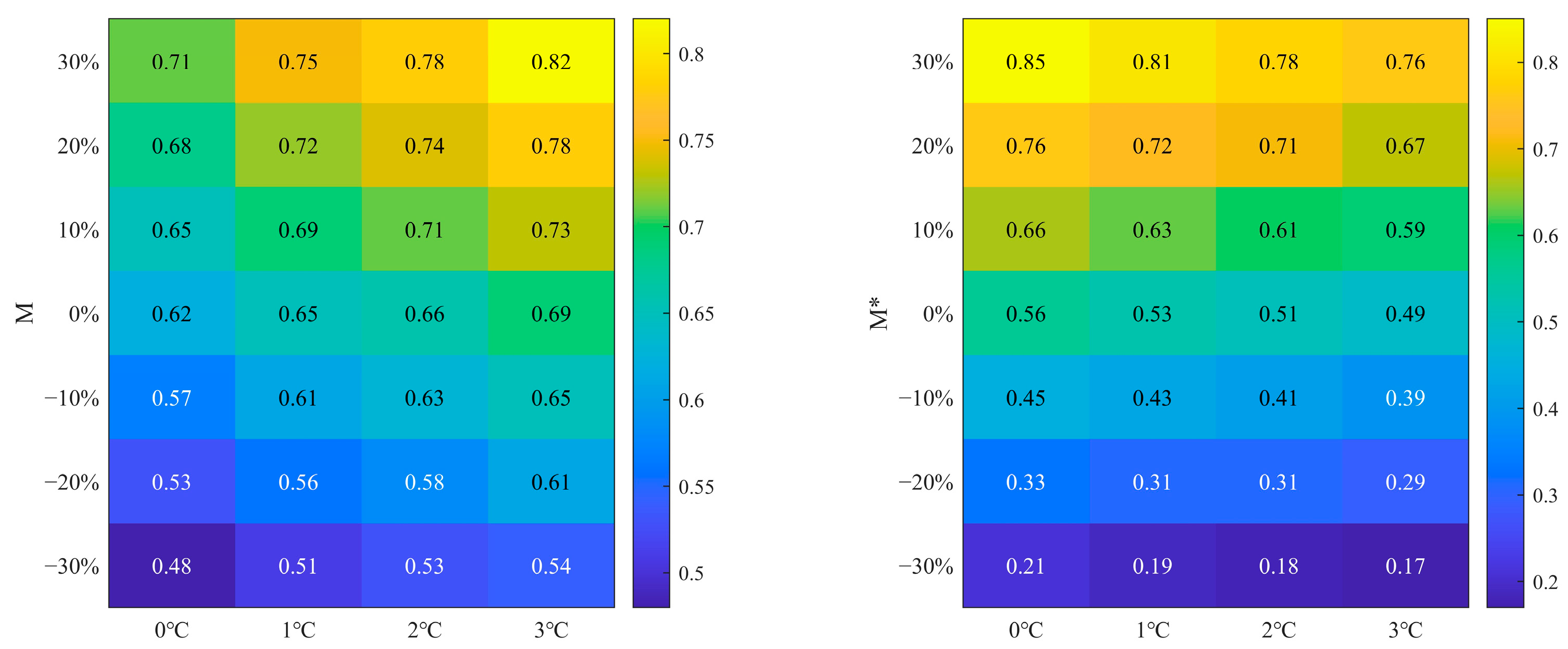
On the basis of previous studies, we explored vegetation dynamics under 28 climatic conditions (Figure 8) [39]. Although the optimal vegetation cover represents an average value for the watershed, and Section 3.3 concludes that the optimal vegetation cover in forested areas of the watershed is less than the actual vegetation cover, the optimal vegetation cover in various parts of the watershed is minimally influenced by the vegetation type. Especially under conditions where the optimal vegetation cover further decreases, given that the forest area in the watershed has not significantly decreased over the past thirty years and there has been no large-scale vegetation die-off, the watershed can be considered homogeneous with respect to the vegetation type. This study posits that, as long as the optimal vegetation cover does not further decrease, exacerbating vegetation water stress, the ecological balance of the watershed will not be disrupted. Moreover, under future climate scenarios, if the average optimal vegetation cover exceeds the actual vegetation cover, the situation will develop favorably, supporting the sustainable use of water resources.

Climate change leads to variations in both M and M*, with M varying between 0.48 and 0.82 and M* varying between 0.21 and 0.85. When the rainfall remains constant, an increase in T results in an increase in M. For a 1 °C rise in T, M increases by 4.11%; for a 2 °C rise, M increases by 6.24%; and for a 3 °C rise, M increases by 10.60%. Conversely, for a rise in T of 1, 2, and 3 °C, there is decrease in M* from 0.53 to 0.51 and finally to 0.49, respectively. With a constant value of T, M or M* increases as the rainfall increases. For example, M* rises from 0.56 to 0.85 when the rainfall increases by 30%; similarly, M rises from 0.62 to 0.71. When there is decrease in the rainfall, the sensitivity to climate change of M* is notably higher than that of M. For example, M* reduces from 0.56 to 0.21 as the rainfall declines by 30%; similarly, M reduces from 0.62 to 0.48.

4. Discussion

4.1. Improvements of the Model

On the basis of previous studies and the characteristics of the study area, we proposed a coupled ecohydrological model with higher accuracy. Su et al. [40] did not explore the effects of the climate on vegetation or the feedback of vegetation on the climate when applying Eagleson’s model to the Hei River Basin. In contrast, in our study, we explored the dynamic thresholds of vegetation under different climatic conditions and discussed whether the vegetation dynamics under different conditions satisfied the ecological balance conditions of the watershed. Cong et al. [41] validated the model by checking whether the optimal vegetation coverage obtained from the simulation was consistent with the trend of the actual vegetation coverage, whereas our validation was completed by fitting the runoff term obtained from the model simulation with the measured runoff, which was demonstrated to fit well. Additionally, our method established cross comparison to assess the accuracies of the hydrological elements using remote sensing-related data and additional field measurements.

Despite these results, our model had several limitations. First, the effect of frozen ground degradation on runoff from the watershed was not considered. The response mechanism of runoff to permafrost degradation remains unclear, and the assumptions made in different studies regarding the impacts of permafrost degradation in different watersheds vary [42,43,44]. Second, most current ecohydrological models do not consider lateral hydrological processes [45]. However, it has also been suggested that the influence of lateral hydrological processes can be attenuated when modeling the long-term average state of ecohydrological equilibrium in a watershed [30].

4.2. Analysis of Vegetation Coverage

Notably, 67.23% of the study region exhibited M* values lower than M, indicating that the current state of vegetation growth within the watershed surpasses the sustainable threshold for watershed development conditions. Regions where M* is lower than M are primarily located in the eastern mountainous forest areas of the watershed, namely subwatersheds A, B, E, and F. Conversely, the regions where M* exceeds M are mainly found in the southwestern grassland zone of subwatersheds C and D. Despite being a drier region with lower precipitation and higher values of T, the grassland zone achieves a certain equilibrium state of water and heat conditions. This allows for the possibility of the equilibrium vegetation coverage surpassing the actual vegetation coverage in the area. Although the forests within the watershed are in relatively humid zones, the dominant woody vegetation in the forested region within the ecohydrological system has a higher water demand. Because forests have experienced a greater decline in precipitation during 1982–2012 when compared to that of grassland areas, additional water stress is imposed on the system. Excessive vegetation coverage can exacerbate the drought conditions within the watershed. According to the ecohydrological optimality approach, functional adaptations within plant communities can mitigate increases in vegetation water stress, even in the presence of local water scarcity [46]. In arid and semiarid regions, it is crucial to pay attention to the balance between vegetation coverage and water consumption. During 1982–2012, the actual vegetation coverage and water consumption both increased. Owing to the greenhouse effect, the rise in T has led to a reduction in M*, relative to the ecohydrological balance. Therefore, when there is no statistically significant change in precipitation, it results in a larger difference between M and M*, exacerbating water stress and aggravating drought issues in arid and semiarid regions.

4.3. Application of the Derived Conclusions

A study has demonstrated that the vegetation coverage in Inner Mongolia is affected differently by precipitation and T on different time scales, and that the main drivers of the coverage of different types of vegetation vary on the same time scale [47]. Therefore, we simulated the vegetation coverage under 28 different climatic conditions to investigate the relationship between vegetation dynamics and climatic factors. Results showed that the vegetation coverage in the Hailar River Basin was positively correlated with precipitation, M was positively correlated with T, and M* was negatively correlated with T, similarly to the results of previous studies [48,49]. We estimated vegetation coverage thresholds and analyzed vegetation dynamics for the different climatic conditions in order to provide a basis for future revegetation activities and to help manage vegetation to cope with the effects of future climate change.

Vegetation change is beneficial to local water resources on over 50% of the global land surface; however, it is detrimental in water-limited regions such as the Hailar River Basin [16]. The Huihe forest in the study area has been restored as a result of the afforestation program, but this has also resulted in M* (0.17) being significantly smaller than M (0.82), exacerbating water depletion. China has implemented a series of afforestation programs since the 1980s [50,51,52]. With such a trend, we suggest considering the vegetation type as well as factors such as water-use efficiency and light-energy utilization when planting [53,54,55]. Studies have shown that water consumption by grasslands is notably lower than that by woodlands, that evergreen forests consume more water than deciduous forests, and that it is preferable to plant vegetation that is native to the area and that requires less water [56]. The light-energy utilization and water-use efficiency of several major vegetation establishment species in the Hailar River Basin were characterized as follows: C. scabra (7.78 mg/g, 0.044 μmol/μmol), L. chinesis (5.71 mg/g, 0.030 μmol/μmol), S. grandis (5.19 mg/g, 0.025 μmol/μmol), and A. frigida (4.54 mg/g, 0.013 μmol/μmol) [57,58]. A selection of vegetation types with high water and light-energy utilization can be effective for optimizing the water use in a watershed. Therefore, the optimal native vegetation types for planting were ranked as follows: C. scabra > L. chinesis > S. grandis > A. frigida > Larix gmelinii > Pinus sylvestris var. mongolica > Betula platyphylla forest.

In regions where water availability is the main factor limiting plant growth, such as arid and semiarid regions, excessive afforestation poses a threat to ecosystem sustainability via the depletion of available water resources. In regions with excessive vegetation coverage, the relationship between vegetation coverage and soil moisture is not linear, but follows a saturation curve [25]. When the vegetation coverage exceeds a critical threshold, the soil moisture reaches a stable value, indicating that excessive planting leads to soil dryness. Over an extended period, soil dryness has several adverse effects on vegetation, such as hindered growth, reduced resilience to drought, and impaired plant regeneration. Therefore, in arid and semiarid regions under specific meteorological conditions, it is crucial to determine the threshold values for the optimal vegetation coverage, and to establish a balanced relationship between the optimal vegetation coverage and the actual vegetation coverage.

This study combined the climate–vegetation–hydrological balance theory with an ecohydrological model to quantify the maximum climate change that the study watershed could tolerate under the constraint of vegetation dynamic thresholds, thereby providing a theoretical basis for addressing future climate change and its implications.

5. Conclusions

In this study, we proposed an improved ecohydrological model that is more applicable to arid and semiarid regions. The main conclusions derived are as follows.

• By modifying the flow term in the water balance equation, the accuracy of the runoff estimation was improved. By validating the soil moisture remote sensing data using multiply data, the application of the model has been promoted.
• The optimal vegetation coverage under the long-term ecohydrological balance for the period of 1982–2012 was calculated. The average vegetation coverage for the entire watershed was 0.62, whereas the average optimal vegetation coverage was 0.56. Regions where the optimal vegetation coverage was lower than the actual vegetation coverage were mainly distributed in the eastern mountainous forest areas of the watershed, namely subwatersheds A, B, E, and F, whereas regions where the optimal vegetation coverage was higher than the actual vegetation coverage were mainly distributed in the southwestern grassland areas of subwatersheds C and D.
• The sensitivity of the optimal vegetation coverage to the vegetation parameters, including $\beta$, $L_t$, and $h_s/h$, was analyzed. It was evident that the optimal vegetation coverage had the least sensitivity to $h_s/h$ and the greatest sensitivity to increases in $\beta$ and decreases in $L_t$, resulting in a higher optimal vegetation coverage.
• The sensitivity of the optimal vegetation coverage to meteorological parameters, including $m_h$, $m_{tb}$, $E_{ps}$, and T, was also analyzed. It was found that the optimal vegetation coverage was most sensitive to $m_h$, and that it increased with increases in $m_h$ and decreased with reductions in $m_{tb}$, $E_{ps}$, and T.
• On the basis of the analysis of climate change using the dynamic threshold of vegetation, it was found that the watershed only achieved an equilibrium state under sustainable development conditions when the rainfall increased by 10%, 20%, and 30% without an increase in T, or when the rainfall increased by 20% with an increase in T of 1 °C.

References

1. Wen, Z.; Wu, S.; Chen, J.; Lü, M. NDVI indicated long-term interannual changes in vegetation activities and their responses to climatic and anthropogenic factors in the Three Gorges Reservoir Region, China. Sci. Total Environ. 2017, 574, 947–959. [Google Scholar] [CrossRef]
2. Ge, W.; Deng, L.; Wang, F.; Han, J. Quantifying the contributions of human activities and climate change to vegetation net primary productivity dynamics in China from 2001 to 2016. Sci. Total Environ. 2021, 773, 145648. [Google Scholar] [CrossRef]
3. Wang, Q.; Ju, Q.; Wang, Y.; Shao, Q.; Zhang, R.; Liu, Y.; Hao, Z. Vegetation Changing Patterns and Its Sensitivity to Climate Variability across Seven Major Watersheds in China. Int. J. Environ. Res. Public. Health 2022, 19, 13916. [Google Scholar] [CrossRef]
4. Zhang, P.; Cai, Y.; He, Y.; Xie, Y.; Zhang, X.; Li, Z. Changes of vegetational cover and the induced impacts on hydrological processes under climate change for a high-diversity watershed of south China. J. Environ. Manag. 2022, 322, 115963. [Google Scholar] [CrossRef]
5. Ma, N.; Szilagyi, J.; Zhang, Y. Calibration-Free Complementary Relationship Estimates Terrestrial Evapotranspiration Globally. Water Resour. Res. 2021, 57, e2021WR029691. [Google Scholar] [CrossRef]
6. Yang, Y.; Donohue, R.J.; McVicar, T.R.; Roderick, M.L. An analytical model for relating global terrestrial carbon assimilation with climate and surface conditions using a rate limitation framework. Geophys. Res. Lett. 2015, 42, 9825–9835. [Google Scholar] [CrossRef]
7. Hidalgo, A.; Tello, L. Modeling and Numerical Simulation of a Vegetation Cover. Math. Comput. Sci. 2021, preprint. [Google Scholar] [CrossRef]
8. Xin, Z.; Xu, J.; Zheng, W. Spatiotemporal variations of vegetation cover on the Chinese Loess Plateau (1981–2006): Impacts of climate changes and human activities. Sci. China Ser. Earth Sci. 2008, 51, 67–78. [Google Scholar] [CrossRef]
9. Deng, Y.; Wang, S.; Bai, X.; Luo, G.; Wu, L.; Chen, F.; Wang, J.; Li, C.; Yang, Y.; Hu, Z.; et al. Vegetation greening intensified soil drying in some semi-arid and arid areas of the world. Agric. For. Meteorol. 2020, 292–293, 108103. [Google Scholar] [CrossRef]
10. Zhu, Z.; Piao, S.; Myneni, R.B.; Huang, M.; Zeng, Z.; Canadell, J.G.; Ciais, P.; Sitch, S.; Friedlingstein, P.; Arneth, A.; et al. Greening of the Earth and its drivers. Nat. Clim. Chang. 2016, 6, 791–795. [Google Scholar] [CrossRef]
11. Chen, C.; Park, T.; Wang, X.; Piao, S.; Xu, B.; Chaturvedi, R.; Fuchs, R.; Brovkin, V.; Ciais, P.; Fensholt, R.; et al. China and India lead in greening of the world through land-use management. Nat. Sustain. 2019, 2, 122–129. [Google Scholar] [CrossRef]
12. Peña-Arancibia, J.L.; Bruijnzeel, L.A.; Mulligan, M.; van Dijk, A.I.J.M. Forests as ‘sponges’ and ‘pumps’: Assessing the impact of deforestation on dry-season flows across the tropics. J. Hydrol. 2019, 574, 946–963. [Google Scholar] [CrossRef]
13. Te Wierik, S.A.; Cammeraat, E.L.H.; Gupta, J.; Artzy-Randrup, Y.A. Reviewing the Impact of Land Use and Land-Use Change on Moisture Recycling and Precipitation Patterns. Water Resour. Res. 2021, 57, e2020WR029234. [Google Scholar] [CrossRef]
14. Spracklen, D.; Arnold, S.; Taylor, C. Observations of increased tropical rainfall preceded by air passage over forests. Nature 2012, 489, 282–285. [Google Scholar] [CrossRef]
15. Bentley, L.; Coomes, D.A. Partial river flow recovery with forest age is rare in the decades following establishment. Glob. Chang. Biol. 2020, 26, 1458–1473. [Google Scholar] [CrossRef]
16. Cui, J.; Lian, X.; Huntingford, C.; Gimeno, L.; Wang, T.; Ding, J.; He, M.; Xu, H.; Chen, A.; Gentine, P.; et al. Global water availability boosted by vegetation-driven changes in atmospheric moisture transport. Nat. Geosci. 2022, 15, 982–988. [Google Scholar] [CrossRef]
17. Zeng, Z.; Piao, S.; Li, L.Z.X.; Wang, T.; Ciais, P.; Lian, X.; Yang, Y.; Mao, J.; Shi, X.; Myneni, R.B. Impact of Earth Greening on the Terrestrial Water Cycle. J. Clim. 2018, 31, 2633–2650. [Google Scholar] [CrossRef]
18. Li, X.; Wang, Y.; Xue, B.; A, Y.; Zhang, X.; Wang, G. Attribution of runoff and hydrological drought changes in an ecologically vulnerable basin in semi-arid regions of China. Hydrol. Process. 2023, 37, e15003. [Google Scholar] [CrossRef]
19. Xue, B.; A, Y.; Wang, G.; Helman, D.; Sun, G.; Tao, S.; Liu, T.; Yan, D.; Zhao, T.; Zhang, H.; et al. Divergent Hydrological Responses to Forest Expansion in Dry and Wet Basins of China: Implications for Future Afforestation Planning. Water Resour. Res. 2022, 58, e2021WR031856. [Google Scholar] [CrossRef]
20. Wu, Y.; Zhang, H.; Lan, T.; Wei, X.; Shao, S.; Zhang, J.; Ding, H. Attribution of runoff variation to climate and human-driven changes in the transition zone between the Qinling Mountains and the Loess Plateau under vegetation greening. Hydrol. Res. 2022, 53, 733–753. [Google Scholar] [CrossRef]
21. Bai, P.; Liu, X.; Zhang, Y.; Liu, C. Assessing the Impacts of Vegetation Greenness Change on Evapotranspiration and Water Yield in China. Water Resour. Res. 2020, 56, e2019WR027019. [Google Scholar] [CrossRef]
22. Zhou, G.; Wei, X.; Chen, X.; Zhou, P.; Liu, X.; Xiao, Y.; Sun, G.; Scott, D.; Zhou, S.-Y.-D.; Han, L.; et al. Global pattern for the effect of climate and land cover on water yield. Nat. Commun. 2015, 6, 5918. [Google Scholar] [CrossRef] [PubMed]
23. Fang, Q.; Wang, G.; Zhang, S.; Peng, Y.; Xue, B.; Cao, Y.; Shrestha, S. A novel ecohydrological model by capturing variations in climate change and vegetation coverage in a semi-arid region of China. Environ. Res. 2022, 211, 113085. [Google Scholar] [CrossRef]
24. Shao, W.; Yang, D.; Sun, F.; Wang, J. Analyzing the Regional Soil-Vegetation-Atmosphere Interaction Using Both the Eagleson and Budyko’s Water Balance Models. Procedia Environ. Sci. 2011, 10, 1908–1913. [Google Scholar] [CrossRef]
25. Zhang, S.; Yang, D.; Yang, Y.; Piao, S.; Yang, H.; Lei, H.; Fu, B. Excessive Afforestation and Soil Drying on China’s Loess Plateau. J. Geophys. Res. Biogeosci. 2018, 123, 923–935. [Google Scholar] [CrossRef]
26. Liang, W.; Bai, D.; Wang, F.; Fu, B.; Yan, J.; Wang, S.; Yang, Y.; Long, D.; Feng, M. Quantifying the impacts of climate change and ecological restoration on streamflow changes based on a Budyko hydrological model in China’s Loess Plateau. Water Resour. Res. 2015, 51, 6500–6519. [Google Scholar] [CrossRef]
27. Zhang, S.; Yang, H.; Yang, D.; Jayawardena, A.W. Quantifying the effect of vegetation change on the regional water balance within the Budyko framework. Geophys. Res. Lett. 2016, 43, 1140–1148. [Google Scholar] [CrossRef]
28. Du, C.; Sun, F.; Yu, J.; Liu, X.; Chen, Y. New interpretation of the role of water balance in an extended Budyko hypothesis in arid regions. Hydrol. Earth Syst. Sci. 2016, 20, 393–409. [Google Scholar] [CrossRef]
29. Wang, D.; Tang, Y. A one-parameter Budyko model for water balance captures emergent behavior in darwinian hydrologic models. Geophys. Res. Lett. 2014, 41, 4569–4577. [Google Scholar] [CrossRef]
30. Li, H.; Liu, L.; Koppa, A.; Shan, B.; Liu, X.; Li, X.; Niu, Q.; Cheng, L.; Miralles, D. Vegetation greening concurs with increases in dry season water yield over the Upper Brahmaputra River basin. J. Hydrol. 2021, 603, 126981. [Google Scholar] [CrossRef]
31. Mo, K.; Cong, Z.; Lei, H. Optimal vegetation cover in the Horqin Sands, China. Ecohydrology 2016, 9, 700–711. [Google Scholar] [CrossRef]
32. Zhang, Y.; Zhao, T.; Shi, C.; Ma, Q. Simulation of Vegetation Cover Based on the Theory of Ecohydrological Optimality in the Yongding River Watershed, China. Forests 2021, 12, 1377. [Google Scholar] [CrossRef]
33. Almalki, R.; Khaki, M.; Saco, P.M.; Rodriguez, J.F. Monitoring and Mapping Vegetation Cover Changes in Arid and Semi-Arid Areas Using Remote Sensing Technology: A Review. Remote Sens. 2022, 14, 5143. [Google Scholar] [CrossRef]
34. Khan, Z.; Khan, Z.; Ahmed, A.; Bazai, M.H. Land use/land cover change detection and prediction using the CA-Markov model: A case study of Quetta city, Pakistan. J. Geogr. Soc. Sci. (JGSS) 2021, 2, 164–182. [Google Scholar]
35. A, Y.; Wang, G.; Liu, T.; Xue, B.; Kuczera, G. Spatial variation of correlations between vertical soil water and evapotranspiration and their controlling factors in a semi-arid region. J. Hydrol. 2019, 574, 53–63. [Google Scholar] [CrossRef]
36. Fang, Q.; Wang, G.; Liu, T.; Xue, B.-L.; A, Y. Controls of carbon flux in a semi-arid grassland ecosystem experiencing wetland loss: Vegetation patterns and environmental variables. Agric. For. Meteorol. 2018, 259, 196–210. [Google Scholar] [CrossRef]
37. Li, J.; Bai, X.; Jin, Y.; Song, F.; Chen, Z.; Cai, L.; Zou, F.; Jiang, M.; Yun, R.; Lv, Z. Recent Intensified Runoff Variability in the Hailar River Basin during the Past Two Centuries. J. Hydrometeorol. 2020, 21, 2257–2273. [Google Scholar] [CrossRef]
38. Fang, Q.; Xin, X.; Guan, T.; Wang, G.; Zhang, S.; Ma, M. Vegetation patterns governing the competitive relationship between runoff and evapotranspiration using a novel water balance model at a semi-arid watershed. Environ. Res. 2022, 214, 113976. [Google Scholar] [CrossRef] [PubMed]
39. Han, D.; Wang, G.; Liu, T.; Xue, B.-L.; Kuczera, G.; Xu, X. Hydroclimatic response of evapotranspiration partitioning to prolonged droughts in semiarid grassland. J. Hydrol. 2018, 563, 766–777. [Google Scholar] [CrossRef]
40. Su, T.; Zhang, B.; He, X.; Shao, R.; Li, Y.; Tian, J.; Long, B.; He, C. Rational Planning of Land Use Can Maintain Water Yield Without Damaging Ecological Stability in Upstream of Inland River: Case Study in the Hei River Basin of China. J. Geophys. Res. Atmos. 2020, 125, e2020JD032727. [Google Scholar] [CrossRef]
41. Cong, Z.; Li, Q.; Mo, K.; Zhang, L.; Shen, H. Ecohydrological optimality in the Northeast China Transect. Hydrol. Earth Syst. Sci. 2017, 21, 2449–2462. [Google Scholar] [CrossRef]
42. Duan, L.; Man, X.; Kurylyk, B.L.; Cai, T.; Li, Q. Distinguishing streamflow trends caused by changes in climate, forest cover, and permafrost in a large watershed in northeastern China. Hydrol. Process. 2017, 31, 1938–1951. [Google Scholar] [CrossRef]
43. Niu, L.; Ye, B.; Ding, Y.; Li, J.; Zhang, Y.; Sheng, Y.; Yue, G. Response of hydrological processes to permafrost degradation from 1980 to 2009 in the Upper Yellow River Basin, China. Hydrol. Res. 2016, 47, 1014–1024. [Google Scholar] [CrossRef]
44. Wang, T.; Yang, H.; Yang, D.; Qin, Y.; Wang, Y. Quantifying the streamflow response to frozen ground degradation in the source region of the Yellow River within the Budyko framework. J. Hydrol. 2018, 558, 301–313. [Google Scholar] [CrossRef]
45. Fatichi, S.; Pappas, C.; Ivanov, V.Y. Modeling plant–water interactions: An ecohydrological overview from the cell to the global scale. WIREs Water 2016, 3, 327–368. [Google Scholar] [CrossRef]
46. Barkaoui, K.; Navas, M.; Roumet, C.; Cruz, P.; Volaire, F. Does water shortage generate water stress? An ecohydrological approach across Mediterranean plant communities. Funct. Ecol. 2017, 31, 1325–1335. [Google Scholar] [CrossRef]
47. Mu, S.; Yang, H.; Li, J.; Chen, Y.; Gang, C.; Zhou, W.; Ju, W. Spatio-temporal dynamics of vegetation coverage and its relationship with climate factors in Inner Mongolia, China. J. Geogr. Sci. 2013, 23, 231–246. [Google Scholar] [CrossRef]
48. Sun, Y.; Guo, P.; Yan, X.; Zhao, T. Dynamics of vegetation cover and its relationship with climate change and human activities in Inner Mongolia. J. Nat. Resour. 2010, 25, 407–414. (In Chinese) [Google Scholar]
49. Xu, X.; Li, X.; Liang, H.; Huang, L. Change in vegetation coverage and its relationships with climatic factors in temperate steppe, Inner Mongolia. Acta Ecol. Sin. 2010, 30, 3733–3743. (In Chinese) [Google Scholar]
50. Lü, Y.; Fu, B.; Feng, X.; Zeng, Y.; Liu, Y.; Chang, R.; Sun, G.; Wu, B. A Policy-Driven Large Scale Ecological Restoration: Quantifying Ecosystem Services Changes in the Loess Plateau of China. PLoS ONE 2012, 7, e31782. [Google Scholar] [CrossRef]
51. Wu, Z.; Wu, J.; Liu, J.; He, B.; Lei, T.; Wang, Q. Increasing terrestrial vegetation activity of ecological restoration program in the Beijing–Tianjin Sand Source Region of China. Ecol. Eng. 2013, 52, 37–50. [Google Scholar] [CrossRef]
52. Xue, B.; Helman, D.; Wang, G.; Xu, C.-Y.; Xiao, J.; Liu, T.; Wang, L.; Li, X.; Duan, L.; Lei, H. The low hydrologic resilience of Asian Water Tower basins to adverse climatic changes. Adv. Water Resour. 2021, 155, 103996. [Google Scholar] [CrossRef]
53. Chen, Y.; Wu, B.; Chen, D.; Qi, Y. Using Machine Learning to Assess Site Suitability for Afforestation with Particular Species. Forests 2019, 10, 739. [Google Scholar] [CrossRef]
54. Liu, Y.; Miao, H.-T.; Huang, Z.; Cui, Z.; He, H.; Zheng, J.; Han, F.; Chang, X.; Wu, G.-L. Soil water depletion patterns of artificial forest species and ages on the Loess Plateau (China). For. Ecol. Manag. 2018, 417, 137–143. [Google Scholar] [CrossRef]
55. Zhou, G.; Xia, J.; Zhou, P.; Shi, T.; Li, L. Not vegetation itself but mis-revegetation reduces water resources. Sci. China Earth Sci. 2021, 64, 404–411. [Google Scholar] [CrossRef]
56. Feng, X.; Fu, B.; Piao, S.; Wang, S.; Ciais, P.; Zeng, Z.; Lü, Y.; Zeng, Y.; Li, Y.; Jiang, X.; et al. Revegetation in China’s Loess Plateau is approaching sustainable water resource limits. Nat. Clim. Chang. 2016, 6, 1019–1022. [Google Scholar] [CrossRef]
57. Fang, Q.; Wang, G.; Xue, B.; Liu, T.; Kiem, A. How and to what extent does precipitation on multi-temporal scales and soil moisture at different depths determine carbon flux responses in a water-limited grassland ecosystem? Sci. Total Environ. 2018, 635, 1255–1266. [Google Scholar] [CrossRef]
58. Cui, Q.Y.; Chen, Z.Z.; Du, Z.C. Characteristics of light energy and water utilization of major plants in semi-arid grasslands. Acta Prataculturae Sin. 2001, 10, 14–21. (In Chinese) [Google Scholar]
Figure 1. Study area.
Remotesensing 16 02132 g001
Figure 2. Soil moisture validation (a) GLDAS against In-situ data; (b) GLDAS against field sampling data.
Remotesensing 16 02132 g002
Figure 3. Runoff validation in the six subwatersheds.
Remotesensing 16 02132 g003
Figure 4. Runoff validation between the six subwatersheds.
Remotesensing 16 02132 g004
Figure 5. Spatial distributions of (a) vegetation coverage, (b) optimal vegetation coverage, and (c) their difference, blue circle represent the Hui-River Forest.
Remotesensing 16 02132 g005
Figure 6. Sensitivity of the optimal vegetation coverage to vegetation parameters (a)   h s / h , (b) β , (c) L t .
Remotesensing 16 02132 g006
Figure 7. Sensitivity of the optimal vegetation coverage to meteorological parameters (a) m h , (b) m t b , (c) E p s and (d) T.
Remotesensing 16 02132 g007
Figure 8. Variations in actual/optimal vegetation coverage in different climatic conditions.
Remotesensing 16 02132 g008