Ground-Based Hyperspectral Estimation of Maize Leaf Chlorophyll Content Considering Phenological Characteristics

Abstract

Accurately measuring leaf chlorophyll content (LCC) is crucial for monitoring maize growth. This study aims to rapidly and non-destructively estimate the maize LCC during four critical growth stages and investigate the ability of phenological parameters (PPs) to estimate the LCC. First, four spectra were obtained by spectral denoising followed by spectral transformation. Next, sensitive bands (R_λ), spectral indices (SIs), and PPs were extracted from all four spectra at each growth stage. Then, univariate models were constructed to determine their potential for independent LCC estimation. The multivariate regression models for the LCC (LCC-MR) were built based on SIs, SIs + R_λ, and SIs + R_λ + PPs after feature variable selection. The results indicate that our machine-learning-based LCC-MR models demonstrated high overall accuracy. Notably, 83.33% and 58.33% of these models showed improved accuracy when the R_λ and PPs were successively introduced to the SIs. Additionally, the model accuracies of the milk-ripe and tasseling stages outperformed those of the flare–opening and jointing stages under identical conditions. The optimal model was created using XGBoost, incorporating the SI, R_λ, and PP variables at the R3 stage. These findings will provide guidance and support for maize growth monitoring and management.

1. Introduction

Chlorophyll is the essential driving force behind light energy conversion and crop growth [1,2]. Leaf chlorophyll content (LCC) plays a significant role in plant photosynthetic efficiency, nutrient content, and crop yield and also indicates plant growth, primary productivity, and carbon use efficiency [3,4,5]. However, traditional chemical methods for determining the LCC require experimental procedures such as weighing, extraction, and assaying, which cause irreversible damage to leaves and are time-consuming and labor-intensive.

Advancements in remote sensing technology have led scientists to deeply appreciate the unique potential of hyperspectral technology for accurately estimating vegetation physiological and biochemical parameters [6,7,8]. As a non-destructive, efficient, and real-time remote sensing monitoring method, hyperspectral technology can use the differences in the absorption and reflection of light energy by chlorophyll in different plants to achieve LCC quantitative estimation [9]. Pan et al. [10] found a high correlation between the derivative spectra of maize leaves at 714 nm and their chlorophyll content. Recent studies have demonstrated the efficacy of employing a diverse array of remote sensing data and physical and empirical models in enhancing the precision of LCC estimation. Gao et al. [11] integrated the PROSPECT and LESS radiative transfer modeling models to comprehensively assess the efficacy of forest LCC estimation at the leaf and canopy scales. Wan et al. [12] proposed using near-infrared reflectance of vegetation to minimize the effects of the canopy structure and soil background in Sentinel-2 and Landsat-7/8 images. This study will further explore the improvement of LCC estimation methods to optimize agricultural production.

Over the past decade, more scientists have integrated the principles of classical spectral indices (SIs) [13] with hyperspectral techniques to estimate the LCC. Concurrently, a continuous influx of new SIs have been proposed. We attempted to summarize these SIs into the following three categories: broadband SIs, narrowband SIs, and optimal spectral indices (SIc). Schlemmer et al. [14] estimated the chlorophyll and nitrogen content of maize leaves at the canopy level using the following three different SIs: the green chlorophyll index (CIgreen), the red edge chlorophyll index (CIrededge), and the MERIS terrestrial chlorophyll index (MTCI). These indices were constructed from the broadbands of the red, green, red edge, and near-infrared (NIR), with CIrededge giving the most favorable results. In addition, the chlorophyll vegetation index (CVI) and the GreenNDVI, constructed based on broadbands, have been shown to have tremendous potential for chlorophyll estimation [15]. Wu et al. [16] compared various band combinations and found that three narrowband vegetation indices, the modified chlorophyll absorption ratio index (MCARI), the MCARI/OSAVI, and the modified simple ratio index (MSR), were influential in estimating the LCC, while eliminating the influence of soil reflectance and non-photosynthetic substances. Jay et al. [17] demonstrated the ability of the structure-insensitive pigment index (SIPI) to estimate the sugar beet LCC. However, since the leaf structure and pigment composition are not precisely the same for different plants, either broadband or narrowband SIs need to be optimized for better estimation [17]. Furthermore, Jiang et al. [18] traversed all two-by-two combinations in the 380–1000 nm band to generate the SIc, compared them with the SIs, and found that the SIc could be used to build a more reliable prediction model for maize anthocyanins.

In exploring vegetation growth and maturation, phenology is regarded as a critical and irreplaceable indicator of climate and natural environmental changes [19,20,21]. The vegetation index seasonal curves are the basis for determining phenological period nodes [22], and familiar methods for determining phenological parameters (PPs) can be categorized into three groups, namely, the threshold method [23], the delayed moving average method [24], and the change-point estimation method [25]. Piao et al. [26] considered ground-based phenology observations as a traditional but beneficial approach, in some cases superior to more advanced remote sensing observations. However, traditional plant phenology research mainly explores the cyclical growth events of plant germination, flowering, and fruiting through field observations, which makes it challenging to obtain PPs that reflect the actual growth status of vegetation [27,28]. Scientists have already applied the combination of vegetation phenology and multispectral data to the study of vegetation type identification and achieved excellent results [29]. However, the cross-study with the hyperspectral field has not been reported. Furthermore, the time-series curves of rice, wheat, and maize plotted by Wu et al. [30] based on four variables, including gross primary production, yielded PPs that differed less under the same crop species. However, the study of PPs for maize LCC inversion has not been reported.

It is noteworthy that the current prediction models of vegetation physiological and biochemical parameters constructed using hyperspectral data still exhibit the following limitations: (1) in the data preprocessing stage, few studies have considered the effect and accuracy of spectral denoising [31], not to mention the precision comparison of different methods; (2) in the modeling stage, most studies usually take only the results of a single spectral transformation [32] as the data source, ignoring the data exploration ability of different spectral transformation methods’ data discovery abilities, and fewer studies use multiple spectral transformation methods at the same time; (3) in the model evaluation stage, the selected indices tend to ignore the evaluation of the overfitting degree [33] of the model, which brings more uncertainty to the generalizability of the model.

In response to the above issues, the LCC at four vital growth stages of maize was estimated using three types of variables, namely, sensitive bands (R_λ), SIs (broadband classical SIs, narrowband classical SIs, and SIc), and PPs derived from 360–1000 nm hyperspectral reflectance data, combined with different spectral transformation methods and modeling approaches. The objectives of this study are (1) to apply the vegetation index seasonal curves from vegetation remote sensing to ground hyperspectral data and explore their potential for LCC estimation, and (2) to explore new parameter combinations and high-accuracy modeling for estimating the LCC of maize leaves at different growth stages based on the improvement of the three shortcomings above. This paper will reference the new application of phenological data in hyperspectral techniques and provide theoretical and decision-making support for modern agricultural management and precision agriculture.

Table A1. Concept abbreviations list.

Category	Concept	Abbreviations
broadband spectral indices	the green chlorophyll index	CIgreen
	the red edge chlorophyll index	CIrededge
	the chlorophyll vegetation index	CVI
	the MERIS terrestrial chlorophyll index	MTCI
critical growth stage of maize	milk-ripe stage	R3
	twelfth leaf stage or flare–opening stage	V12
	sixth leaf stage or jointing stage	V6
	tasseling stage	VT
evaluation metrics	interquartile range	IQR
	R-square	R2
	root mean square error	RMSE
	root mean square error of calibration	RMSEC
	root mean square error of validation	RMSEV
	relative prediction deviation	RPD
	standard deviation	SD
feature variable selection method	competitive adaptive reweighted sampling	CARS
	genetic algorithm	GA
	successive projections algorithm	SPA
	uninformative variables elimination	UVE
fundamental variables	phenological parameters	PPs
	sensitive bands	Rλ
	optimal spectral indices	SIc
	spectral indices	SIs
machine learning	gradient-boosting decision trees	GBDTs
	random forest	RF
	random forest regression	RFR
	support vector machine	SVM
	support vector regression	SVR
	extreme gradient boosting	XGBoost
narrowband spectral indices	the modified chlorophyll absorption ratio index	MCARI
	the modified simple ratio index	MSR
	the structure-insensitive pigment index	SIPI
phenological parameters	amplitude of season	AOS
	gross spring greenness	GSG
	net spring greenness	NSG
	the peak value of season	POS
	rate of growth	ROG
regression models	machine learning regression models for LCC estimation	LCC-ML
	multivariate regression models for LCC estimation	LCC-MR
	univariate regression models for LCC estimation	LCC-UR
	machine learning	ML
	machine learning regression	MLR
spectral denoising method	Gaussian filter	GF
	moving average	MA
	median filter	MF
	Savitzky–Golay	SG
the original and transformed spectra	the discrete wavelet transform spectra	DWT
	the first derivative spectra	FD
	the original spectra	OS
	the standard normal variate spectra	SNV
other	leaf area index	LAI
	leaf chlorophyll content	LCC
	near-infrared	NIR

Note: In alphabetical order of the category and abbreviations.

in the Appendix A all of the concept abbreviations utilized in this article.

2. Materials and Methods

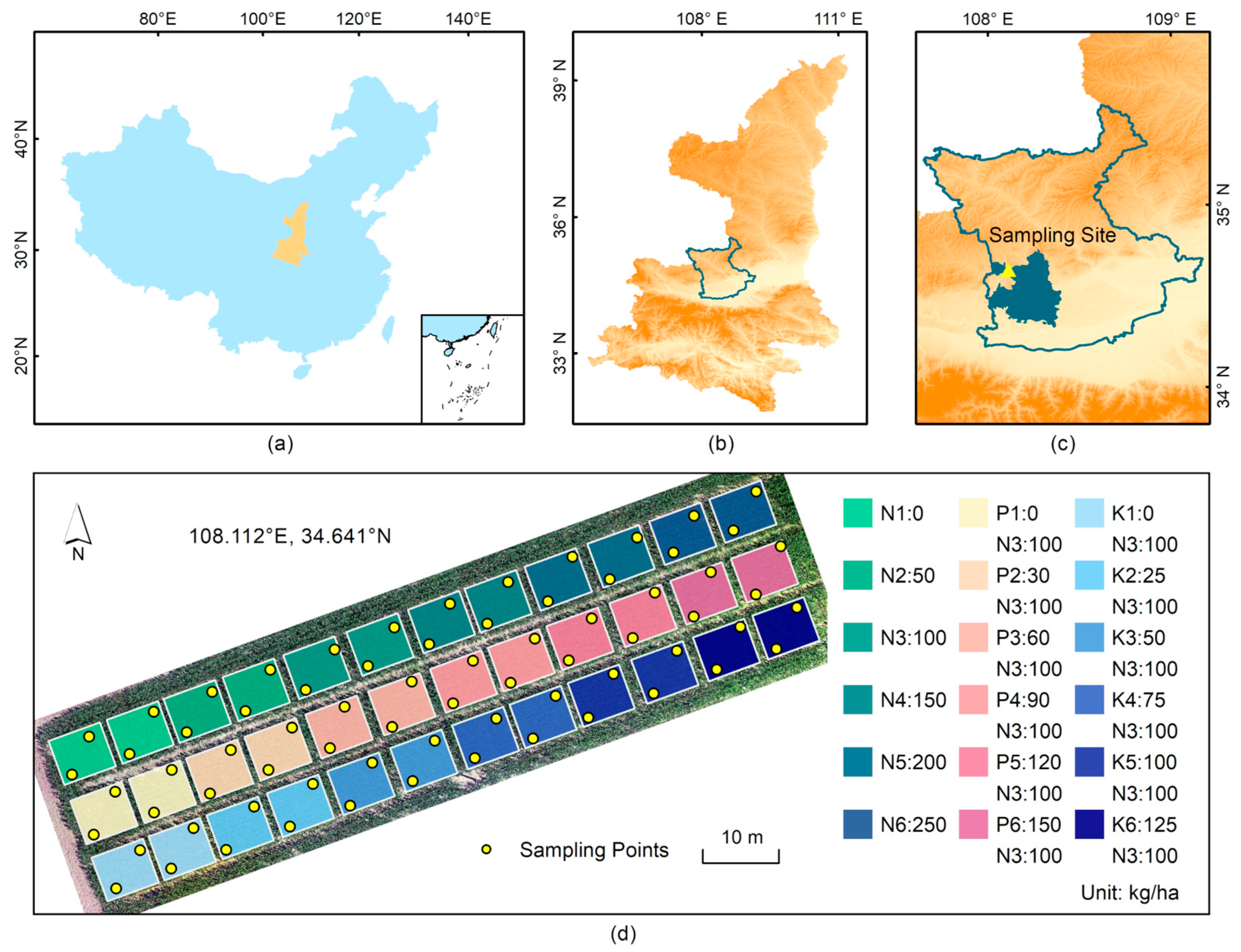
2.1. Experimental Design

The field trial site, as depicted in Figure 1, is located in Qinan Village, Liangshan Town, Qian County, Xianyang City, Shaanxi Province (108.112°E, 34.641°N), in the northern part of the Guanzhong Plain, a typical agricultural region in China. The area has an average elevation of 980.11 m and features low terrain in the southeast and high terrain in the northwest, with slight slopes. The geomorphological type is loess tableland, and the soil type is loam. The climate is mild, with distinct seasons. It belongs to the temperate continental monsoon climate, with an average annual temperature of 13.2 °C and an average annual precipitation of 500–600 mm. The local crop ripening system is two years of triple ripening or one year of ripening, and the main crops include wheat, maize, and oilseed rape.

The field trial was conducted from April 2021 to August 2021, and the crop variety was “Shandan 2001” maize. The trial started on April 20 and was divided into 36 plots, each with two sampling points on the diagonal, with a plot area of 56 m² (7 m × 8 m). Different fertilization treatments were applied to each plot to increase the data variability and improve the generalizability of the maize LCC modeling. In this trial, three treatments of N, P, and K were set up, and each treatment had six levels and two replications. The pure nitrogen application rate of the N fertilizer treatment was 0, 50, 100, 150, 200, and 250 kg/ha; the K₂O application rate of the K fertilizer treatment was 0, 25, 50, 75, 100, and 125 kg/ha; the P₂O₅ application rate of the P fertilizer treatment was 0, 30, 60, 90, 120, and 150 kg/ha. The fertilizers for each treatment were applied once before maize planting, without follow-up, and other management measures were the same as those used in the local high-yield field. Figure 1d shows the fertilization treatments and sampling points in the field trials.

Maize leaves were sampled at the following four vital growth stages: V6 (sixth leaf stage or jointing stage) on June 10, V12 (twelfth leaf stage or flare–opening stage) on June 29, VT (tasseling stage) on July 31, and R3 (milk-ripe stage) on August 30 [34]. At each stage, three leaves in good growth condition were collected from the maize plant’s upper, middle, and lower parts at each of the 72 sampling points in all plots.

2.2. Data Collection

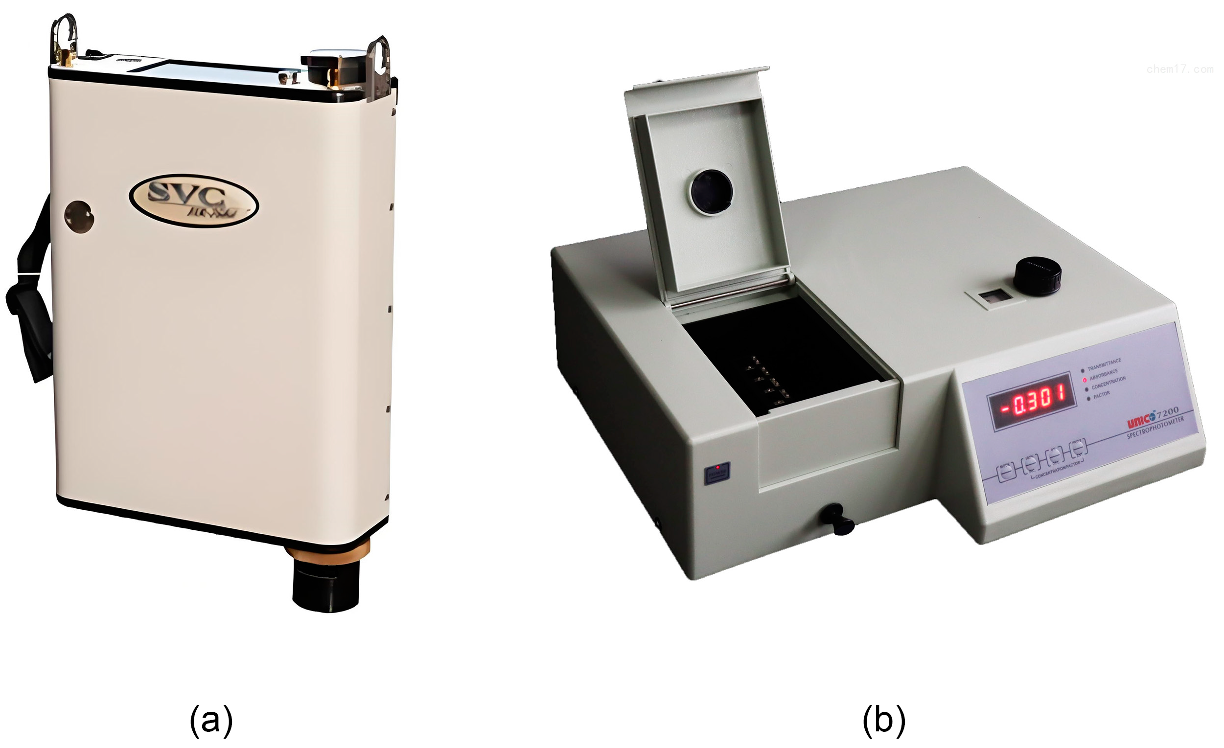
2.2.1. Hyperspectral Data Acquisition

The hyperspectral data of the maize leaves were measured with the SVC HR-1024i (Spectra Vista Corporation, Poughkeepsie, NY, USA) high-performance portable non-imaging ground spectrometer. The instrument covers 350 to 2500 nm, offering varying spectral resolutions across the following different band ranges: 3.5 nm for 350–1000 nm, 9.5 nm for 1000–1850 nm, and 6.5 nm for 1850–2500 nm [18]. The spectral data were collected indoors, and reference plate correction was performed before testing at 0.5 h intervals. Three healthy, pest-free leaves were collected at each sampling point, and two spectral curves were determined for each leaf’s tip, center, and base. The hyperspectral data for each sampling point was the average of the 18 spectral curves. Finally, all spectral curves were resampled to 1 nm in the SVC HR1024i software. Based on previous studies [14,18,35], the spectral range of this study was determined to be 360–1000 nm. Figure 2a shows the SVC HR-1024i device.

2.2.2. Leaf Chlorophyll Content Determination

The maize leaf LCC was determined using the spectrophotometric method. The acquisition of hyperspectral data was synchronized with the LCC determination. Leaves were wiped clean, avoiding veins and hyperspectral measurement sites, and the central part of the leaf was selected and cut into debris. For each sampling site, approximately 0.2 g of leaf debris was weighed, added to 95% ethanol, and placed in a dark room for 2–3 days until the leaves turned white. After filtration and volume fixation of 25 mL, the absorbance at 649 and 665 nm was determined with a spectrophotometer. The chlorophyll concentration (mg/L) was calculated according to Equation (1) and combined with the mass of the leaves and the volume of the extracted liquid to calculate the LCC (mg/g). In Equation (1), $C_T$, $C_a$, and $C_b$ are the total chlorophyll concentration, chlorophyll a, and chlorophyll b, and $A_{\mathsf{\lambda }}$ is the absorbance at λ nm [36]. Finally, the 3σ principle was used to detect outliers in the LCC values at each growth stage, and there was an outlier in each of the V6, VT, and R3 stages. The hyperspectral data of the sample points where the outliers were located were excluded accordingly and not included in this study. The visible spectrophotometer is shown in Figure 2b.

$$C_T=C_a+C_b=\left(13.95\times A_{665}-6.88\times A_{649}\right)+(24.96\times A_{649}-7.32\times A_{665})$$

(1)

2.3. Model-Independent Variable Determination

2.3.1. Spectral Denoising and Transformation

In this study, four spectral denoising methods, the Gaussian filter (GF), median filter (MF), moving average (MA), and Savitzky–Golay (SG), were compared using the R-square (R²) and root mean square error (RMSE) as evaluation metrics. The GF is a linear smoothing filter whose probability density function obeys normal distribution. The segment size of the GF method in this study was set to 3 [37]. The basic principle of the MF is to replace the center value with the median of all values in the sliding filter window, and we set the segment size to 3 based on previous research [38]. In the sliding filter window, the center value is averaged with the other values in the window, and the average value is taken as the center value, which is the process of MA implementation. The segment size of the MA method in this study was set to 3 [37]. The SG is a polynomial smoothing algorithm based on the principle of least squares with the polynomial order set to 2 and the number of left/right side points set to 5 [18]. This part was implemented by Unscrambler X 10.4 [39].

The spectra obtained by denoising were the original spectra (OS). In this study, the OS was transformed to obtain the first derivative spectra (FD), the standard normal variate spectra (SNV), and the discrete wavelet transform spectra (DWT). These transformations allowed for the extraction of the R_λ, SIs, and PPs as modeling-independent variables. Among them, the FD is the first-order derivative of the OS and represents the rate of change in the OS. The FD can display more spectral details due to the amplification of the OS curves by the FD [40,41]. The fundamental premise of the SNV is to standardize the hyperspectral data of each sample, with a mean of 0 and a standard deviation of 1. The SNV can broaden the spectrum’s absorption properties while maintaining the OS’s fundamental characteristics [42]. Moreover, the DWT decomposes the leaf spectrum into high- and low-frequency components. The low-frequency component is retained, while the high-frequency component is thresholded. Layer-by-layer decomposition is then performed in the low-frequency component, generating multiple sub-signals. The DWT has the advantage of highlighting refined features, making it suitable for spectral feature extraction [43]. The concurrent application of disparate transformed spectra permits the synthesis of the spectral information generated by disparate methodologies, thereby furnishing a more comprehensive corpus of raw data to estimate the LCC. This part was carried out using Matlab R2023a [44].

2.3.2. Spectral Indices (SIs) and Phenological Parameters (PPs)

Spectral indices are closely related to the plant growth status and leaf pigment content. This study selected five broadband SIs and five narrowband SIs, highly correlated with the LCC, as the independent variables. The calculation equations and references for each index are shown in

Table 1. Classical spectral indices and phenological parameters.

SIs	Equations/Definition	References
CIgreen	${(R}_{NIR}/R_{green})-1$	[14]
CIrededge	${(R}_{NIR}/R_{rededge})-1$	[14]
CVI	${(R}_{NIR}/R_{green})/{(R}_{red}/R_{green})$	[15]
GreenNDVI	${(R}_{NIR}-R_{green})/{(R}_{NIR}+R_{green})$	[15]
MTCI	${(R}_{NIR}-R_{rededge})/{(R}_{rededge}+R_{red})$	[14]
MCARI	$[\left({\rho }_{700}-{\rho }_{670}\right)-0.2\left({\rho }_{700}-{\rho }_{550}\right)]({\rho }_{700}/{\rho }_{670})$	[8]
MCARI/OSAVI	$[\left({\rho }_{700}-{\rho }_{670}\right)-0.2\left({\rho }_{700}-{\rho }_{550}\right)]({\rho }_{700}/{\rho }_{670})/$ $\left[\right(1+0.16\left)\right({\rho }_{800}-{\rho }_{670})/({\rho }_{800}+{\rho }_{670}+0.16\left)\right]$	[16]
MSR	$({\rho }_{800}/{\rho }_{670}-1)/\sqrt{{\rho }_{800}/{\rho }_{670}+1}$	[16]
OSAVI	$(1+0.16)({\rho }_{800}-{\rho }_{670})/({\rho }_{800}+{\rho }_{670}+0.16)$	[16]
SIPI	$({\rho }_{850}-{\rho }_{445})/({\rho }_{850}+{\rho }_{680})$	[17]
AOS	the difference between the maximum and the mean value line	[45]
GSG	the area enclosed by the time series and its endpoints	[45]
NSG	the area enclosed by the time series and its mean value line	[45]
POS	the maximum value of the time series	[45]
ROG	the average positive slope of the time series	[45]

Note: Band range: green: 540–560 nm; red: 660–680 nm; red edge: 690–750 nm; NIR: 780–800 nm; R represents the average reflectance over a range of bands, and ρ represents the reflectance of a particular band.

. Among them, the band ranges of the broadband SIs were determined by the spectral curve characteristics of the maize leaves at each growth stage and referring to related studies [14]. In addition, due to the characteristics of the hyperspectral data with many narrow bands, it is essential to explore the most suitable optimized spectral index (SIc). Therefore, this study calculated the DSI, NDSI, and RSI for any two-band combination in the 360–1000 nm band range. The SIc was determined based on the principle of maximum correlation.

In this study, we attempted to introduce PPs into a maize LCC estimation model to explore their capability to invert maize physiological and biochemical parameters. Phenology, a cyclical pattern of organismal growth and activity, and its application in LCC estimation has not been reported. For this study, we generated time-series curves by fitting the NDVI data on a sample-by-sample basis for different transformed spectra, where the x-axis represents the number of days and the y-axis represents the NDVI value. In the fitting process, the R3 and V6 stage data were repeated once at both ends to ensure that the edge data were adequately considered. We referred to the mathematical algorithms of Xue et al. [45] to extract the following five PPs from the time-series curves: the amplitude of season (AOS), the gross spring greenness (GSG), the net spring greenness (NSG), the peak value of season (POS), and the rate of growth (ROG). As defined in Table 1, these parameters indicate the plant growth amplitude, peak greenness, plant vigor, gross greenness, and net greenness [45]. This part was realized using Matlab R2023a [44].

2.3.3. Feature Variable Selection

Ordinary feature variable selection methods include the competitive adaptive reweighted sampling (CARS), genetic algorithm (GA), successive projections algorithm (SPA), and uninformative variables elimination (UVE). The CARS and SPA methods determine the selection result using the RMSE minimization principle. Moreover, UVE performs the selection by setting a threshold, but the same number of variables cannot be obtained with the same threshold. Suppose there is no guarantee that the number of variables used is equal. In that case, it is impossible to compare the effect of the LCC estimation of different models and growth stages. Furthermore, some scholars have proposed that CARS only applies to PLSR algorithms [46]. In contrast, the GA method has the ability to optimize globally. It can guarantee an equal number of variables by counting the variables with the highest frequency of occurrence through multiple operations. GA is an optimization strategy for stochastic global search in a high-dimensional space with the following four main configurations: coding, fitness function, genetic operator, and operating parameters. The GA performs the variable selection process by simulating genetic selection and natural elimination during biological evolution, which includes genetic coding, population initialization, selection, crossover, and mutation [47]. The GA population consists of random coding genes, and the response function is used to evaluate each coding gene, inserting more suitable individuals into the population and replacing the worst individuals. The parameters of the GA in this study were set as follows: number of populations, 50; crossover probability, 50%; mutation probability, 1%; genetic generations, 100 [48]. Finally, the results of 100 independent runs of the GA were used as feature variables in the model. In the multivariate modeling process, the input variables were the same for each model to facilitate the evaluation of the model performance. The procedure was implemented in Matlab R2023a [44].

2.4. Regression Analysis Method

After the 3σ principle method to remove outliers, the maize LCC in each growth stage was ranked in ascending order, and stratified random sampling was performed at a ratio of 3:1 to divide the calibration set and validation set. There were 53, 54, 53, and 53 samples in the modeling set for the V6, V12, VT, and R3 growth stages, respectively, and 18 samples in the validation set for each growth stage. This study used three types of regression analyses, including univariate linear and nonlinear regression, multivariate linear regression, and multivariate machine learning (ML) regression, to estimate the maize LCC and evaluate the potential of the PPs in the LCC estimation. All regression analysis methods were performed in Matlab R2023a [44].

Random forest regression (RFR) is an integrated learning algorithm that combines Bagging with the decision tree algorithm [49]. In the training phase, RFR uses the Bootstrap function to obtain several different sub-training data from the input calibration dataset to train different decision trees separately [50]. In the statistical phase, the final regression result is determined by the combined decision result of each binary decision tree, which improves the model’s robustness and stability by statistically analyzing many decision trees [51]. The random forest (RF) model construct based on TreeBagger must set the two critical parameters of the number of decision trees, “ntree”, and the minimum number of leaves, “mtry” [52], set to 550 and 1/3 of the sample size by debugging.

Support vector regression (SVR) is a classic early ML model that focuses on finding an optimal regression plane to which all data have the shortest distance [53]. In SVR, the dimensionality of the input data is independent of the computational complexity, which can solve nonlinear high-dimensional problems well [54]. It has demonstrated high predictive performance in numerous studies. To construct the support vector machine (SVM) using the Libsvm 3.32 software package, two significant parameters, the penalty coefficient (C) and the kernel function parameter (γ) [55], must be set. These parameters were set by performing a grid search in the range of [10-2, 10-1, 1, 10, 100] and [10-4, 10-3, 10-2, 10-1, 1, 10] to determine the optimal results.

Extreme gradient boosting (XGBoost) is a scalable and parallelizable ML method for efficient operations and an improved algorithm for gradient-boosting decision trees (GBDTs) [56]. XGBoost 1.4.0 uses first- and second-order derivatives for leaf node splitting optimization, and thus does not require a specific definition of the loss function. This makes XGBoost suitable for various loss functions and ideal for different applications. In addition, to control the complexity of the model and prevent overfitting, XGBoost introduces a regularization term, which improves the model’s fitting and generalization capabilities [57]. This study used the CV function to determine that the max_depth was 3, the min_child_weight was 2, the subsample was 0.8, the colsample_bytree was 0.8 [58], and the other parameters were adopted as default values.

2.5. Model Evaluation Metrics

In this research, the R-square (R²), root mean square error of calibration (RMSEC), root mean square error of validation (RMSEV), and relative prediction deviation (RPD) were chosen to evaluate the maize LCC estimation models. The R² is a dimensionless coefficient that reflects the extent to which the dependent variable is explained by the independent variable in the regression relationship. The RMSEV is used to quantify the accuracy of the model, and when the RMSEV/RMSEC > 1.5, the model is overfitted [59,60]. The RPD is the ratio of the sample standard deviation (SD) to the RMSE. Moreover, an RPD < 1.4 indicates that the model is unable to predict the variables; 1.4 ≤ RPD < 1.8 indicates that the model can implement a rough prediction of the variable; 1.8 ≤ RPD < 2.0 indicates that the model can implement a reasonable prediction of the variable; 2.0 ≤ RPD < 2.5 indicates that the model can implement high-precision prediction; an RPD > 2.5 indicates that the model is capable of reproducing the measured LCC values [61]. This study suggests that a high-precision LCC estimation model should have a high R² and a low RMSEV, and satisfy the two essential conditions of RPD > 2 and RMSEV/RMSEC ≤ 1.5.

3. Results

3.1. Statistical Analysis of LCC

Table 2. Statistics of actual leaf chlorophyll content at each growth stage of maize (V6 presents the sixth leaf stage or jointing stage; V12 presents the twelfth leaf stage or flare–opening stage; VT presents the tasseling stage; R3 presents the milk-ripe stage; the same as below).

Datasets	Growth Stages	Sample Numbers	Range	Mean	Standard Deviation	Coefficient of Variation/%
Calibration set	V6	53	2.13–4.24	3.27	0.44	13.56
	V12	54	1.99–4.72	3.43	0.54	15.73
	VT	53	2.41–4.68	3.59	0.53	14.82
	R3	53	1.85–5.50	3.33	0.78	23.59
Validation set	V6	18	2.26–4.23	3.28	0.49	15.04
	V12	18	2.41–4.52	3.43	0.52	15.06
	VT	18	2.60–4.79	3.62	0.56	15.36
	R3	18	1.77–5.49	3.38	0.85	25.29

presents the statistical results of the actual LCC of maize at various growth stages. The calibration and validation sets demonstrated high consistency and similarity across all statistical indexes. As the maize matured, the LCC exhibited an overall increasing, then decreasing trend, with the VT stage having the highest mean value and the V6 stage having the lowest. The distribution of the maize LCC ranged from 1.77 to 5.50, while the coefficient of variation was between 13.56% and 25.29%. Specifically, the standard deviation and coefficient of variation in the maize LCC increased fluctuatingly over time and peaked at stage R3. This indicates that the maize LCC was more discretized and variable at this stage, resulting in more diverse data.

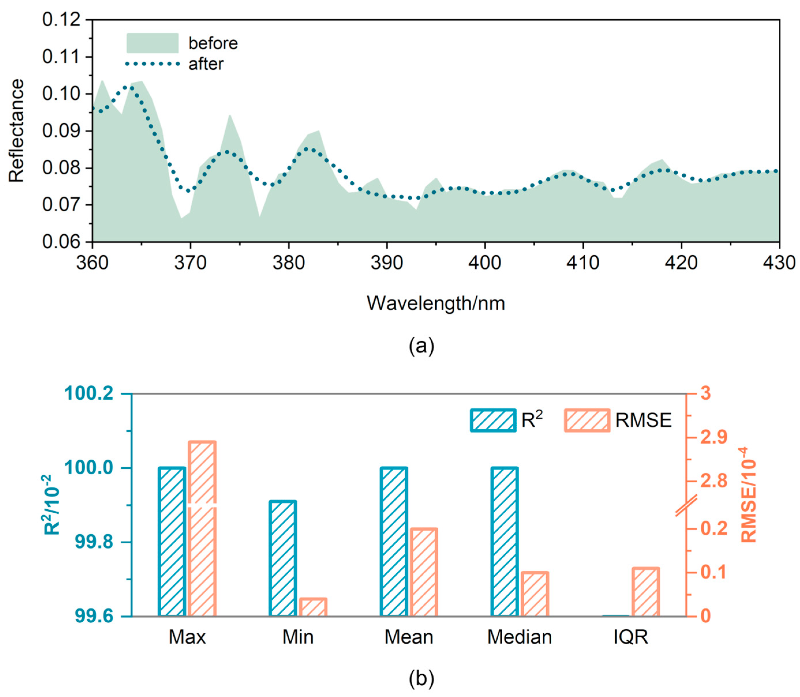
3.2. Spectral Denoising

This study applied four denoising methods, the GF, MF, MA, and SG, to the spectral data. The statistical results showed that, overall, there was very little difference between the R² and RMSE of the four denoising methods. Specifically, in the 360–1000 nm band, the R² of all four methods was very close to 1, and the minimum value reached 0.9599. Additionally, all the RMSE values were very close to 0, with a maximum value of only 0.0031, indicating that the four methods have preserved the information of the original data to the maximum extent and have not introduced any additional errors. Therefore, in detail, we compared the maximum, minimum, median, and interquartile range (IQR) of the R² and RMSE of the four methods. The results showed that the SG method had a significantly smaller minimum value of the R², and its maximum value of the RMSE was also relatively more significant. However, there was almost no significant difference between the other methods. The above results indicated that the SG method was slightly inferior to the other three methods regarding the R² and RMSE, which may be related to the parameter settings. Finally, we chose the GF method, which had the best overall performance, as the denoising method and the results of its spectral processing as the OS. Figure 3a depicts a reflectance comparison between the unprocessed and GF denoised spectra within the 360–430 nm range, with sample point No. 1 as an example. The evaluation results of the GF method are shown in Figure 3b.

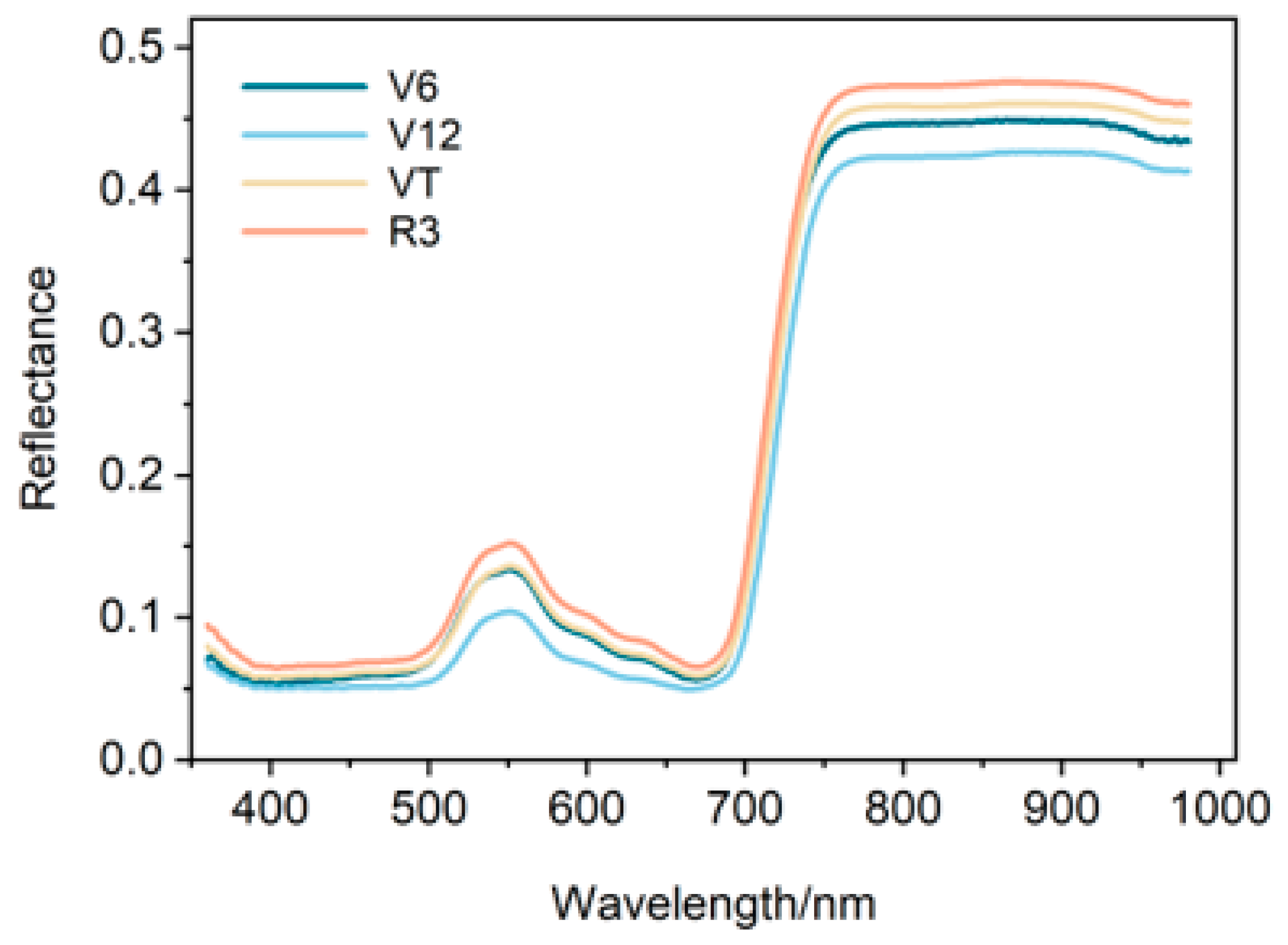
3.3. Spectral Curves of Maize Leaves

The spectral curves of the maize leaves at various growth stages are displayed in Figure 4, with each band’s reflectance indicating the average reflectance of all sample points within it. The overall spectral reflectance followed the R3 > VT > V6 > V12 pattern. Throughout each growth stage, the maize leaves displayed consistent features. Specifically, there were two chlorophyll absorption bands at 360–520 nm and 620–720 nm, resulting in the lowest reflectance of 0.05, which is attributed to the characteristics of the maize chlorophyll in absorbing blue and red light. Additionally, a weak reflectance peak at 520–620 nm was observed, with a corresponding highest reflectance of 0.15. Between 690 and 750 nm, the spectral reflectance increased sharply. It formed a “red edge” due to near-infrared wavelength reflection by the leaf cells. Moreover, a near-infrared high-reflectance platform was formed between 780 and 1000 nm, with all of the spectral reflectance exceeding 0.41.

3.4. Correlation between LCC and Spectral Reflectance

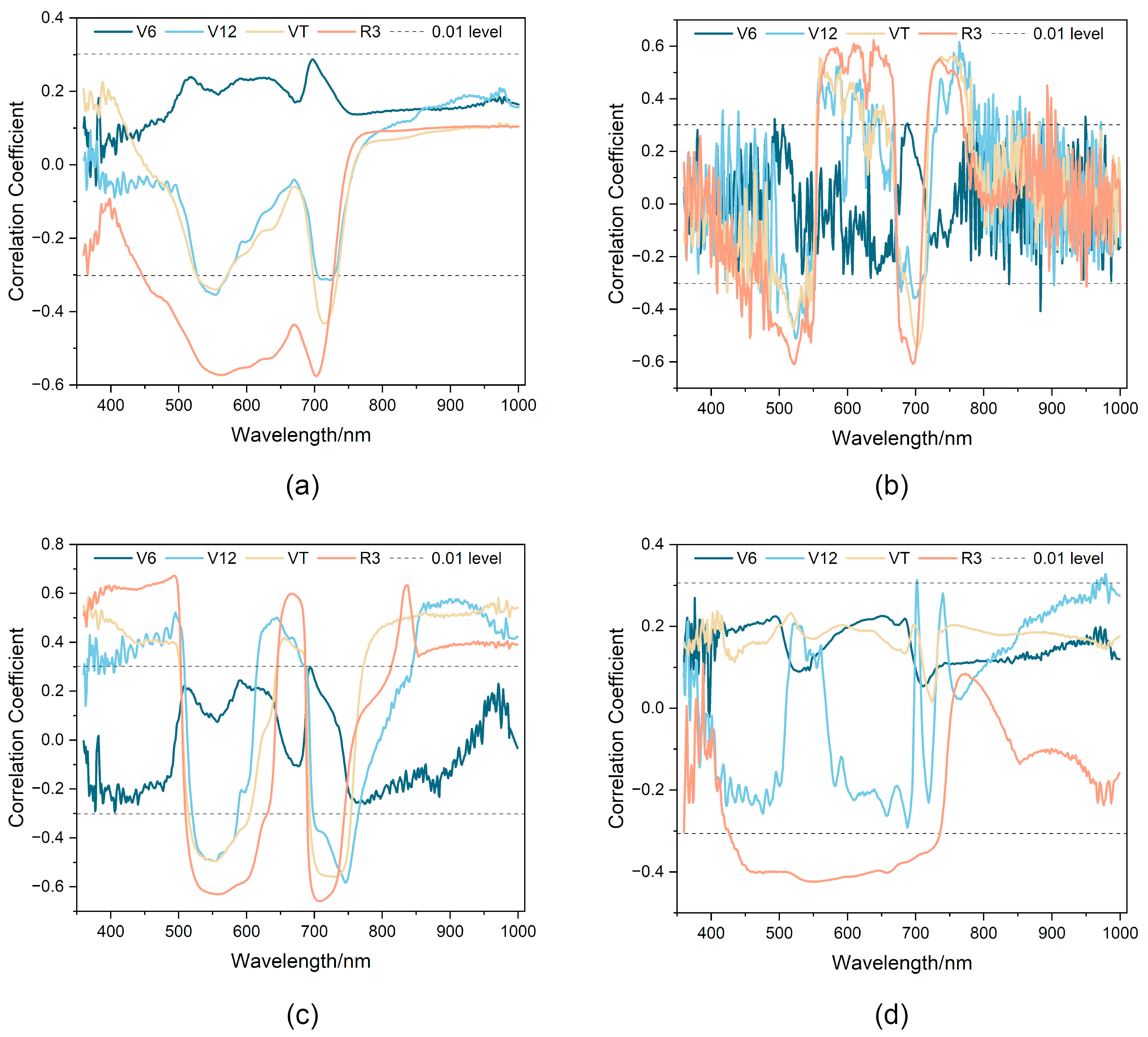
3.4.1. Correlation between LCC and Single-Band Spectrum

Figure 5 depicts the correlation between the maize LCC and various spectra within the 360–1000 nm range. As illustrated by Figure 5a, the correlation curves of the OS were primarily above zero during the V6 stage, while displaying mainly negative correlations in the V12, VT, and R3 stages. During the V6 stage, the OS exhibited a negative correlation in the 370–380 nm band region, with a positive correlation throughout the remaining bands. In contrast, during the V12, VT, and R3 stages, the OS exhibited a positive correlation within the 750–1000 nm spectral band and predominantly showed a negative correlation within the remaining bands. The number of bands in which the correlation coefficients of each growth stage passed the 0.01 significance level test, was 0 in the V6 stage, 68 in the V12 stage, 80 in the VT stage, and 282 in the R3 stage. The highest correlation coefficients for each stage were 0.29, −0.35, −0.43, and −0.58, respectively, corresponding to spectral bands at 697, 554, 714, and 703 nm. These bands were situated at the weak reflectance peak and red edge, as shown in Figure 4. This suggested a correlation between these positions’ spectra and the LCC.

Figure 5b–d illustrate the correlation of the FD, SNV, and DWT with the LCC in maize across various growth stages. At the V6 stage, the number of bands passing the significant level test of 0.01 increased from zero to nine after the OS was transformed to the FD. Figure 5b shows the bands near 500, 700, and 950 nm above the 0.01 level line. At the V12 stage, the SNV increased significantly correlated bands to 491. Figure 5c demonstrates that the spectral reflectance within 360–510 nm, 520–580 nm, 620–680 nm, 700–770 nm, and 850–1000 nm bands exhibit significant correlation with the LCC at the 0.01 level. At the VT stage, the highest number of significantly correlated spectra at the SNV reached 564. The R3 stage exhibited the most significantly correlated spectra with the numbers 282, 299, 547, and 312 at the OS, FD, SNV, and DWT. Figure 5a,d show that the significantly correlated spectra at stage R3 were much more than at the other three stages. After employing various spectral transformations, the maximum correlation coefficients for the V6, V12, VT, and R3 stages increased to −0.41 in the FD, 0.62 in the FD, 0.82 in the SNV, and 0.67 in the SNV, respectively. The above suggested noticeable differences in the ability of various spectral transformation methods to explore information and that all four spectra analyzed in this study enhanced the correlation with the maize LCC at differing growth stages and across various wavelength ranges.

3.4.2. Correlation of LCC with Classical SIs or PPs

Figure 6 depicts the correlation between 10 SIs or five PPs and the LCC across various maize growth stages and spectral conditions. The image indicates varying correlations between the maize LCC and SIs or PPs based on the spectral conditions and growth stages. At the V6 stage, on average, only four parameters passed the significance test at a 0.05 significance level in the OS, FD, and SNV. Meanwhile, in the DWT, no parameters passed the significance test. In the OS and DWT, fewer parameters passed the significance test at stages V12 than in the FD and SNV. At the VT stage, 40.00% of the parameters for the OS and 86.67% for the SNV passed the significance test, with most of them being at the 0.01 level. However, the parameters for the FD and DWT were almost zero at the VT stage. At the R3 stage, 37 parameters passed the significance test in the OS, SNV, and DWT, while only four parameters were in the FD.

The study found that the highest correlation coefficients were observed at the V6, V12, VT, and R3 stages with values of 0.33, 0.67, 0.70, and 0.86, corresponding to the following parameters: the ROG in the FD, GreenNDVI in the SNV, CIrededge in the OS, and CIrededge in the OS. All of the OS, SNV, and DWT parameters of the SIs passed the significance test at the 0.01 level in the R3 stage, except for the MSR value, which was not present in the SNV. Figure 6 demonstrates higher correlations for the SIs in both the OS and DWT at the R3 stage and in the SNV at the V12, VT, and R3 stages. Similarly, the PPs displayed higher correlations in the OS and DWT at the R3 stage and the SNV at the V6 and VT stages. Overall, spectral transformations enhanced the correlation of several SIs and PPs with the maize LCC, and the performance of the PPs was inferior to that of the SIs.

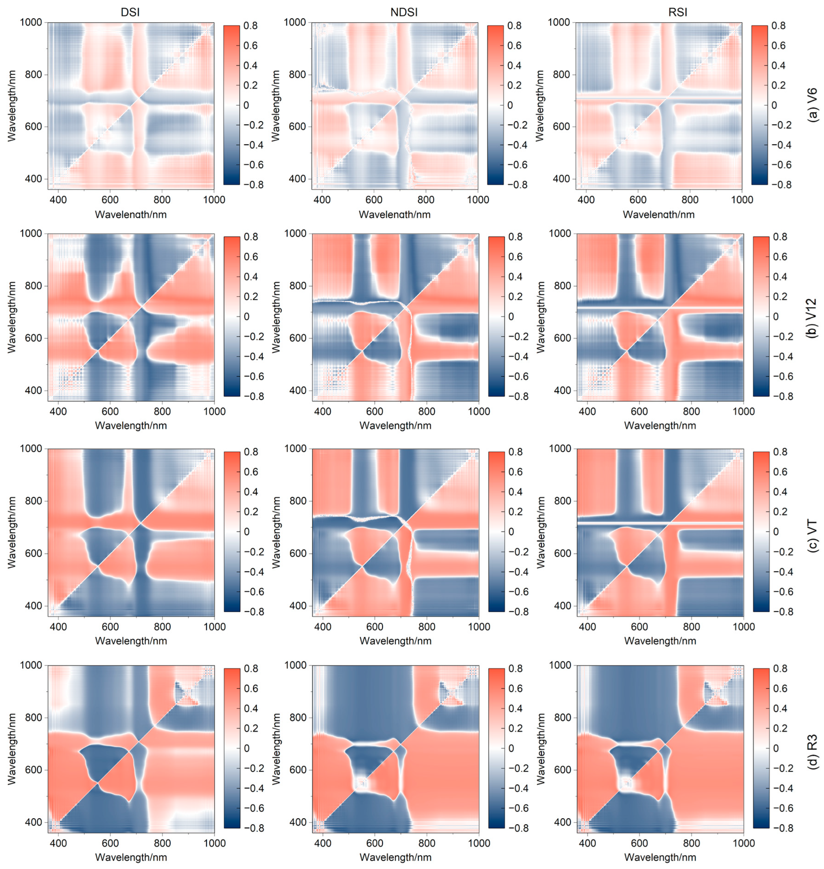
3.4.3. Correlation between LCC and SIc

This study constructed the DSI, RSI, and NDSI using various two-band OS, FD, SNV, and DWT combinations for maize leaves at each growth stage within 360–1000 nm. The transformed spectra that yielded the highest average correlation coefficients at each growth stage were chosen to generate contour maps of the correlation coefficients of the SIc, as illustrated in Figure 7. Figure 7a–c feature the SNV at the V6, V12, and VT stages, while Figure 7d showcases the DWT at the R3 stage. The white areas indicate the absence of any corresponding SIc or where the correlation coefficient is close to zero. In aggregate, the V6 stage correlates weakly with the LCC, while the other stages exhibit only minor differences. At the V6 stage, SNV_DSI proved to have the most effective SIc, while SNV_RSI, SNV_RSI, and DWT_RSI took the lead at stages V12, VT, and R3, with respective average correlation coefficients of 0.23, 0.43, 0.46, and 0.51. The highest correlation coefficients for each growth stage were 0.52, 0.62, 0.62, and 0.70, and the corresponding SIc and band positions were DSI_(956,946), RSI_(764,763), RSI_(367,972), and RSI_(370,460).

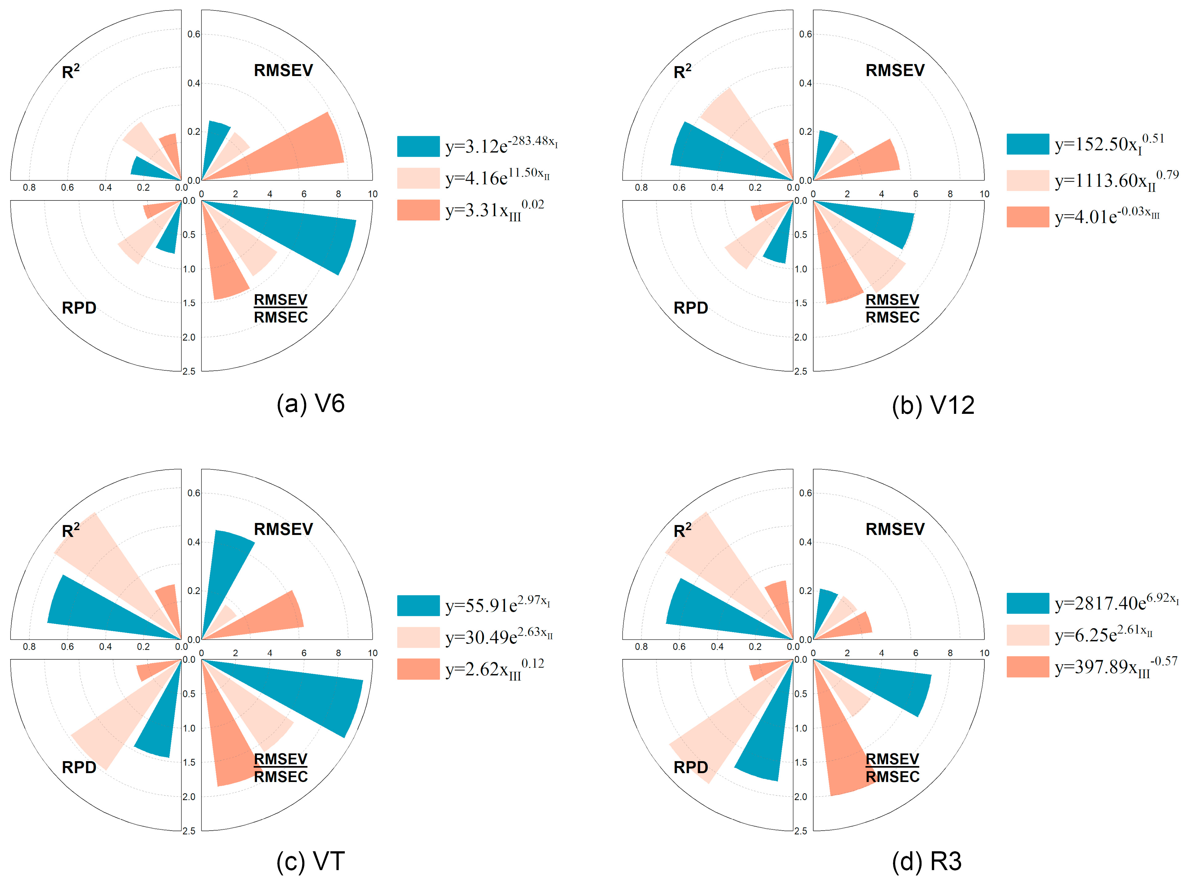
3.5. Univariate Regression Model for LCC Estimation (LCC-UR)

To compare and evaluate the ability of different parameters in estimating the maize LCC independently, we selected the parameters with the highest correlations at each growth stage, including the R_λ (FD_R₈₈₃, FD_R₇₆₄, SNV_R₃₆₇, and SNV_R₄₉₃), the SIs (SNV_DSI_(956,946), FD_DSI_(764,627), SNV_RSI_(367,972), and SNV_DSI_(514,701)), and the PPs (FD_ROG, DWT_AOS, SNV_AOS, and DWT_NSG). These were used as independent variables to construct univariate regression models. The established models included the following five types: primary, quadratic, power, exponential, and logarithmic. We evaluated the accuracy of each model and determined the best models for each growth stage, as shown in Figure 8, along with their expressions and accuracy evaluation parameters.

At the V6 stage, the model based on the independent variable SNV_DSI_(956,946) achieved the highest estimation accuracy, with an R² of 0.3770 and an RMSEV of 0.2412 for the validation set. Moving to the V12 stage, the models built from FD_R₇₆₄ and FD_DSI_(764,627) yielded higher R² values of 0.6521 and 0.5951 and lower RMSEV values of 0.2085 and 0.2042. At the VT stage, the independent variable SNV_RSI_(367,972) produced the highest R² of 0.8126 and the lowest RMSEV of 0.1757. At stage R3, the independent variables SNV_R₄₉₃ and SNV_DSI_(514,701) demonstrated effectiveness, with R² values of 0.6759 and 0.8165 and RMSEV values of 0.2121 and 0.2188, respectively. Figure 8 illustrates that the models’ accuracy in the V6 growth stage is lower than in the remaining stages.

Figure 8 displays the RPD and RMSEV/RMSEC values of each model used to evaluate the comprehensive performance and overfitting of the models. The models built at the V6 and VT stages had RPD values of less than 1.4, indicating they could not predict the maize LCC. On the contrary, models constructed by the R_λ and SI at stages VT and R3 showed RPD values greater than 1.4, suggesting that they predicted the maize LCC with a rough approximation. The models constructed based on the SI at the R3 stage yielded an RPD value greater than 2.0, indicating its high-precision prediction ability. However, it should not be overlooked that all of the LCC-UR models exhibited a much larger RMSEV/RMSEC than 1.5, indicating severe overfitting issues.

The models shown in Figure 8 used independent variables extracted only from the transformed spectra, highlighting the potential of spectral transformation to uncover valuable information. The most accurate models at each growth stage were all power and exponential function models, indicating that the relationship between the maize LCC and variables is nonlinear. Furthermore, power and exponential functions provided a better explanation of this relationship. Regarding the LCC estimation, the regression model created using the independent variable SI performed the best. This result implied that the SI has more potential for estimating the maize LCC because it combines data from both spectra. The R_λ had the second-best performance, while the PPs exhibited the worst performance. This suggests that differences in phenological information at the leaf scale may not be significant, and the R_λ and PPs cannot estimate the maize LCC independently.

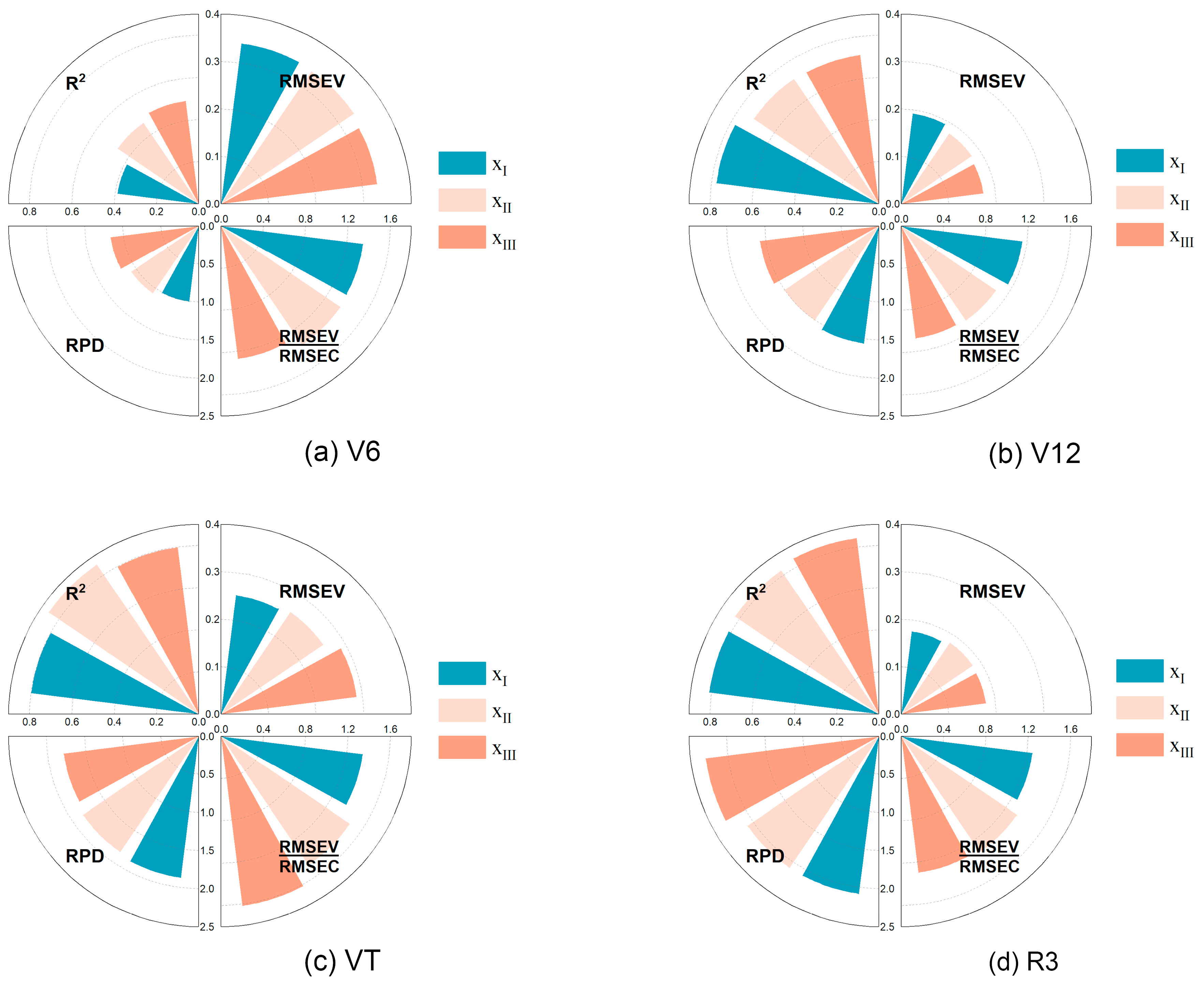
3.6. Multivariate Regression Model for LCC Estimation (LCC-MR)

Due to the correlation between the SIs and maize LCC and their performance in the LCC-UR model, the SIs were utilized as the primary characterizing variables. The optimal R_λ and PPs were combined with the SIs to construct the LCC-MR models. For each growth stage, 52 parameters derived from four transform spectra—including five broadband SIs, five narrowband SIs, and the three SIc—were utilized as inputs for the GA. Then, the GA was executed independently 100 times, and the top 10 variables selected with the highest frequency were identified as the primary characterizing variables in each growth stage. Furthermore, we sequentially added the R_λ and the PPs with the highest correlation to each growth stage to determine the optimal combination of parameters for estimating the maize LCC.

Table 3. The characteristic variables at each growth stage.

Growth Stages	Characteristic Variables
	SIs	Rλ	PPs
V6	OS_RSI, OS_DSI, OS_NDSI, FD_OSAVI, FD_SIPI, FD_MSR, FD_RSI, FD_DSI, SNV_NDSI, DWT_MCARI/OSAVI	FD_R883	FD_ROG
V12	OS_DSI, FD_GreenNDVI, FD_DSI, DWT_MCARI, DWT_MCARI/OSAVI, DWT_CIgreen, DWT_GreenNDVI, DWT_RSI, DWT_DSI, DWT_NDSI	FD_R764	DWT_AOS
VT	OS_RSI, OS_DSI, FD_MCARI, FD_DSI, SNV_MCARI/OSAVI, SNV_CIrededge, SNV_RSI, SNV_DSI, SNV_NDSI, DWT_MTCI	SNV_R367	SNV_AOS
R3	OS_DSI, OS_NDSI, FD_CIgreen, FD_RSI, FD_NDSI, SNV_RSI, SNV_DSI, SNV_NDSI, DWT_RSI, DWT_NDSI	SNV_R493	DWT_NSG

displays the defining variables for each growth stage.

3.6.1. Multivariate Linear Model

The evaluation parameters for the multivariate linear model at each growth stage are illustrated in Figure 9. Results x_I, x_II, and x_III correspond to the inputs of the SIs, SIs + R_λ, and SIs + R_λ + PPs, respectively. Figure 9 indicates that multivariate linear models are much more accurate than the univariate ones. The V6 stage showed an average R² of 0.4482 and an average RMSEV of 0.3367, displaying general performance. In stages V12 and VT, the model’s precision improved compared to the preceding stage, presenting average R² values of 0.7349 and 0.8182 and average RMSEV values of 0.1820 and 0.2667. Ultimately, in the R3 stage, the model’s accuracy peaked with a mean R² of 0.8264 and an RMSEV of 0.1792. With the exception of the x_III at the V12 stage, all RPD values for the models in stages V12 through R3 exceeded 1.8, whereas all model RPD values for stage R3 were more than 2.0. This indicated that the model in the R3 stages can perform high-precision predictions. Furthermore, all RMSEV/RMSEC values were less than 1.5, except for x_III in the V12 stage, with little indication of overfitting.

Among all of the models, 25% satisfied the criterion of RPD > 2 and RMSEV/RMSEC ≤ 1.5, with general performance. Half of the models showed improved accuracy with the addition of the R_λ to the SIs, while a quarter of the models improved with the reintroduction of the PPs. The models with the highest accuracies in the V6, V12, and R3 stages were constructed using the SIs + R_λ + PPs, whereas the best-performing models in the VT stage were based on the SIs. This suggests the ability of the R_λ and PPs to enhance the estimation accuracy in multivariate linear models. Given the limitations of multivariate linear models, we will explore machine learning models in subsequent studies.

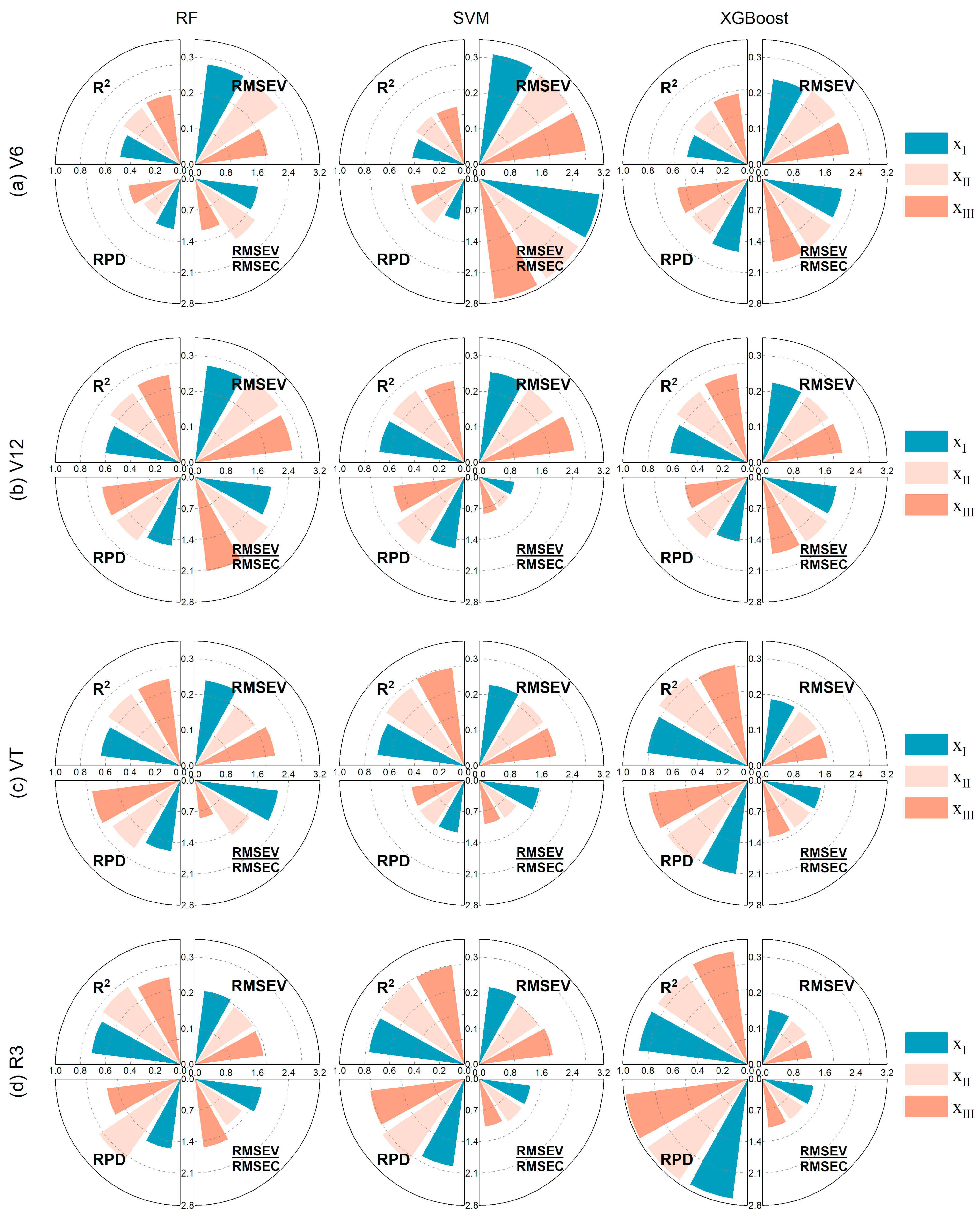
3.6.2. Machine Learning (ML) Model

Since the most practical combination of spectral parameters for estimating the maize LCC was unknown, and considering the superiority of machine learning regression (MLR) in estimating crop physiological and biochemical parameters [8,35,52], we developed the LCC-ML model utilizing the RF, SVM, and XGBoost algorithms. We combined ten selected SIs determined by the GA with the R_λ and PPs as independent variables. The model’s accuracy evaluation parameters at each growth stage are presented in Figure 10.

At the V6 stage, the RF and SVM models that exhibited superior performance were constructed based on the spectral parameter combination of the SIs + R_λ + PPs, resulting in R² values of 0.5637 and 0.4629, with corresponding RMSEV values of 0.2062 and 0.3017. The XGBoost model, constructed using the SIs, outperformed the others in the V6 stage, achieving an R² value of 0.4892 and an RMSEV of 0.2410.

At the V12 stage, the RF model achieved the highest accuracy based on the spectral parameter combination of the SIs + R_λ + PPs, with an R² value of 0.7092 and an RMSEV of 0.2748. The top-performing SVM and XGBoost models resulted from the combination of the SIs + R_λ, with R² values of 0.6953 and 0.6863 and an RMSEV of 0.2510 and 0.2240, and the two models outperformed the others at the V12 stage.

At the VT stage, the RF and XGBoost models with the highest accuracy were constructed based on the spectral parameter combination of the SIs + R_λ + PPs, with R² values of 0.7002 and 0.8118 and RMSEV values of 0.2269 and 0.1843. The SVM model achieved superior performance by implementing the SIs + R_λ combination, resulting in an R² of 0.7574 and an RMSEV of 0.2186, respectively. Notably, the XGBoost model outperformed throughout the stage.

At the R3 stage, the RF and SVM models performed best with the spectral parameter combination of the SIs + R_λ + PPs and SIs + R_λ, producing R² values of 0.7019 and 0.7909 and RMSEV values of 0.1933 and 0.2009, respectively. The XGBoost model achieved the highest accuracy in the R3 stage when using the SIs + R_λ + PPs, with an R² of 0.9118 and an RMSEV of 0.1406.

Figure 10 displays the RPD and RMSEV/RMSEC values for each growth stage. During stage V6, only the RF model was capable of generating a preliminary estimation of the maize LCC (1.4 ≤ RPD < 1.8), whereas all of the models were overfitted at this stage (RMSEV/RMSEC > 1.5). At the V12 stage, the SVM model can implement a reasonable prediction of the maize LCC (1.8 ≤ RPD < 2.0) using the SIs + R_λ spectral parameter combination. However, all of the RF and XGBoost models exhibited overfitting (RMSEV/ RMSEC > 1.5). In the VT stage, the maize LCC was predicted with a high accuracy (2.0 ≤ RPD < 2.5) by all of the XGBoost models, whereas the spectral parameter of the SIs exhibited overfitting. In the R3 stage, every XGBoost model demonstrated the ability to reproduce the measured LCC values accurately (RPD > 2.5). Furthermore, all of the SVM and XGBoost models exhibited no overfitting (RMSEV/RMSEC ≤ 1.5).

Overall, the R3 stage proved to be the most effective for estimating the maize LCC, and six models demonstrated high-precision prediction capability (RPD > 2.0, RMSEV/RMSEC ≤ 1.5). By contrast, only zero, zero, and two models performed well during the V6, V12, and VT growth stages. The XGBoost was the top-performing model for predicting the maize LCC, with five models meeting the high accuracy criteria (RPD > 2.0, RMSEV/RMSEC ≤ 1.5) for all of the growth stages. Among the models that met the criteria of RPD > 2.0 and RMSEV/RMSEC ≤ 1.5, there were one, four, and three models constructed based on the spectral parameters of the SIs, SIs + R_λ, and SIs + R_λ + PPs, respectively. The most exceptional of all of the models was the XGBoost model, which was constructed based on the spectral parameter combination SIs + R_λ + PPs in the R3 stage. It had an R² of 0.9118, an RMSEV of merely 0.1406, an RPD of 2.7662, and an RMSEV/RMSEC of 1.2592.

4. Discussion

4.1. Effect of Spectral Transformations on Chlorophyll Estimation

The selected spectral transformation methods increased the correlation coefficients between the OS and maize LCC. Specifically, the FD increased the correlation coefficients by up to 73.76%, the SNV by up to 64.46%, and the DWT by up to 45.10% at different growth stages. Additionally, the SNV increased the number of bands passing the 0.01 significance level test by 423, 484, and 265 at the V12, VT, and R3 stages. The selected spectral transformation methods can reveal the correlation between the spectral data and vegetation growth status, as previously demonstrated in studies [62,63,64]. The FD can eliminate the effect of parallel background values and make the location of spectrally sensitive bands visible through amplification [40,41]. The SNV reduces the effects of the solid particle size, surface scattering, and spectral range variations on diffuse scattering and broadens the absorption properties of the spectrum [42,65]. The DWT generates the raw data coefficients by transforming the eigenvalues of the detailed and approximated signals, preserving most of the raw data features [43]. Accordingly, the univariate estimation models of the maize LCC were constructed based on the principle of highest correlation. The transformed spectra showed superior performance compared to the OS, and high-precision predictions (RPD > 2.0) were achieved using the SNV at the R3 stage. In the future, the FD, SNV, and DWT may continue to be effective spectral transformation methods, with the SNV being particularly promising.

4.2. Estimating Chlorophyll Using SIs, R_λ, and PPs

As a whole, the potential of the univariate estimation of the maize LCC was SIs > R_λ > PPs, where the SIs include broadband SIs, narrowband SIs, and SIc, and in terms of the correlation with the maize LCC, it was the SIc > broadband SIs > narrowband SIs. Luo et al. developed pigment content estimation models for the dwarf mosaic virus infection of maize based on the R_λ, SIs, and SIc, respectively, and the results showed that the SIc was more effective than the SIs and R_λ [66], which was consistent with the results of this study. However, Zhao et al. [67] found that the broadband use of averaging band information leads to the loss of critical information available in specific narrow bands. The broadband SI ranges in our study were adjusted based on the maize leaf spectral curves and previous research [14,15] to enhance the prediction accuracy for the broadband SIs, leading to the opposite result. PPs are critical in macro-studies such as climate change [26,68] and vegetation classification [30]. Bolton and Friedl improved the accuracy of a county-scale maize yield prediction model in the US by introducing a phenology indicator based on the vegetation index [20]. However, this study found that the PPs could not independently estimate the maize LCC (RPD < 1.4). This may be due to the low frequency of the field trials, resulting in inaccurate time-series curves. However, a frequency of trials that is too high would deviate from the original purpose of the rapid estimation of the maize LCC. Balancing the relationship between the estimation accuracy and practical application is an important direction for future research. In addition, the study scale and geographic location may also be important factors influencing the differences in maize phenology, which will also be considered in the future. The broadband SIs with the most potential to estimate the maize LCC identified in this study were the CIrededge and GreenNDVI, the narrowband SIs were the MCARI and SIPI, and the PPs were the NSG and POS. Furthermore, this paper’s findings align with Schlemmer et al.’s [14] conclusion that the CIrededge is more effective in estimating chlorophyll.

While some LCC-UR models capable of high-precision prediction of the LCC (RPD > 2.0) have been available in the R3 stage, all of the LCC-UR models suffer from severe overfitting (RMSEV/RMSEC > 1.5), which results in poor generalizability in practical use. Therefore, to further explore more superior model parameter combinations, we input the SIs, SIs + R_λ, and SIs + R_λ + PPs into the multivariate linear model and the LCC-ML model, respectively. Research has shown that using SIs obtained from multiple spectral transformation methods rather than a single spectrum led to the better inversion of physiological and biochemical parameters [69]. Therefore, we utilized the SIs obtained from all spectral transformations, after feature variable selection by the GA, as model-independent variables. The accuracy of half of the multivariate linear models was improved by adding the Rλ to the SIs, and the accuracy of one-fourth of the models was enhanced by reintroducing the PPs. The optimal parameter combinations for the modeling were the SIs + R_λ + PPs, SIs + R_λ + PPs, SIs, and SIs + R_λ + PPs for the V6, V12, VT, and R3 stages, respectively. Among these models, only those in the R3 stage could make high-precision predictions (RPD > 2.0). The multivariate linear model, built by combining the SIs, R_λ, and PPs, performed the best (R² = 0.8423, RMSEV = 0.1796, and RPD = 2.2991). It was worth noting that none of the multivariate linear models were overfitted (RMSEV/RMSEC ≤ 1.5), except one model in the VT stage. As for the LCC-ML model, the accuracies of 83.33% of the models were enhanced by introducing the R_λ alongside the SIs, while 58.33% of the models saw improvements upon reintroducing the PPs. The best parameter combinations for each stage were the SIs for the V6 stage, the SIs + R_λ for the V12 stage, the SIs + R_λ + PPs for the VT stage, and the SIs + R_λ + PPs for the R3 stage. Additionally, for the LCC-ML models, nine models made high-precision predictions (RPD > 2.0), and three models were significantly predictive (RPD > 2.5). Among them, the most potent predictive model was constructed using XGBoost (R² = 0.9118, RMSEV = 0.1406, and RPD = 2.7622) and the variables SIs + R_λ + PPs. Overall, the model’s predictive performance improved after introducing the R_λ and PPs. Jiang et al. discovered that combining the R_λ + SIs + SIc into the model was better for estimating the anthocyanins in maize leaves than using a single parameter or a combination of two parameters [18]. This finding was consistent with the results of our study.

The results indicated that the LCC-ML model provided the most accurate estimation, followed by the multivariate linear model, and the LCC-UR model performed the worst. The power and exponential functions showed the highest accuracy for the LCC-UR in all growth stages, but their RMSEV/RMSEC values were too high for practical applications. Only 25% of all multivariate linear models achieved highly accurate predictions, whereas the ML model demonstrated the capacity to reproduce the actual LCC values. The ML models achieved average R² and RPD values of 0.6819 and 1.6233, with an average RMSEV of 0.2298, and only a few individual models displayed overfitting at the VT and R3 stages. The XGBoost model at the R3 stage provided the highest accuracy in predicting the LCC. The ML model’s exceptional performance is due to its utilization of various algorithms and models to thoroughly explore the hyperspectral data’s potential patterns and features, automating the learning and prediction process [70]. The RF addresses overfitting by introducing randomness and maintains high accuracy even with limited datasets. This is due to its ease of parallelization and lack of the need for dimensionality reduction to handle high-dimensional data [71]. Gao et al. [72] used Bayesian optimization in LCC estimation to debug the parameters of the RF method. They obtained a maximum RPD value of 3.21, which is larger than the 2.20 we derived. The SVM can transform the optimal hyperplane into a quadratic programming problem, which provides advantages in dealing with low-sample, high-dimensional, nonlinear, and classification problems [11]. The maximum value of the RPD for all of the SVM models in this study reached 2.22, which is higher than the 2.06 derived by Xiaoyan et al. [73]. According to the study, XGBoost was more stable and accurate than other LCC-UR and LCC-MR models at all growth stages of maize, making it an ideal model for maize LCC estimation [55]. Additionally, the XGBoost model was also superior in estimating other crop growth parameters, such as the leaf area index (LAI) [74] and water content [75].

4.3. Effects of Different Growth Stages on Chlorophyll Estimation

In this study, we developed LCC estimation models for four critical growth stages of maize, each exhibiting distinct LCC estimation performances. At stages V6, V12, VT, and R3, the XGBoost model based only on the SIs (R² = 0.4892, RMSEV = 0.2410, and RPD = 1.6477), the SVM model using the SIs + R_λ (R² = 0.6953, RMSEV = 0.2510, and RPD = 1.8272), the XGBoost model with the SIs + R_λ + PPs (R² = 0.8118, RMSEV = 0.1843, and RPD = 2.2367), and the XGBoost model using the SIs + R_λ + PPs (R² = 0.9118, RMSEV = 0.1406, and RPD = 2.7662) demonstrated the highest LCC estimation accuracy. Except for the V6 stage, there was no overfitting indication (RMSEV/RMSEC ≤ 1.5) in the above models. Overall, the accuracy of the LCC-UR and LCC-MR at each growth stage was, in descending order of the stage, the R3, VT, V12, and V6. This indicates that different growth stages affect the estimation of the LCC in maize, which is consistent with the findings of Schlemmer et al. [14]. Although there were spectral transformations, the accuracy of both the LCC-UR and LCC-MR models was lower at the V6 and V12 stages compared to the R3 and VT stages. This is because V6 and V12 are nutrient growth stages, where the relatively low chlorophyll content and rapid changes in leaf morphology and stomatal density may affect the light absorption and reflection characteristics [76,77]. The R3 and VT stages performed better with the same modeling approach and variables. Guo et al. observed that the correlation between the maize LCC and vegetation index consistently increased across the 11 time points from July 7 to September 30 [78]. Moreover, the model accuracy in our study showed a corresponding improvement from June 10 to August 30. Notably, the coefficient of variation in the actual values of the maize LCC (Table 2) increased fluctuatingly over time, peaking at R3. This significant variation in the LCC values may contribute to the enhanced performance of the estimation model [79].

4.4. Challenges and Future Research

The optimal XGBoost model developed in this study had an RPD of 2.7622, higher than that Yin et al. reported [80]. However, it is difficult to evaluate the model objectively by calculating statistical metrics. Therefore, in the future, the baseline algorithm can be introduced as a comparative criterion to evaluate the model accuracy in the same study [81]. It is necessary to combine XGBoost with the grasshopper optimization algorithm (GOA), the particle swarm optimization (PSO), the whale optimization algorithm (WOA) [82], and other optimization algorithms in order to further improve the estimation accuracy of the model. Furthermore, a model for estimating the LCC based on unmanned aerial vehicle (UAV) data, which considers phenological characteristics, should be developed to demonstrate the potential of the PPs at the canopy scale. Finally, future studies should consider including data from different geographical locations to improve the model’s generalizability.

5. Conclusions

This study estimated the maize LCC of the V6, V12, VT, and R3 stages using ML methods (RF, SVM, and XGBoost) based on the 360–1000 nm OS and spectral-transformed data (FD, SNV, and DWT). The study first constructed the LCC-UR models using the R_λ, SIs, and PPs to evaluate their independent estimation ability. Then, the GA was used to conduct feature variable selection for the SIs. Subsequently, the LCC-MR models were constructed based on the SIs, SIs + R_λ, and SIs + R_λ + PPs, respectively, to analyze the impact of various variable combinations on the model estimation performance. The study drew the following main conclusions:

(1) All three of the transformed spectra could improve the correlation of the spectral data with the maize LCC and showed more significant superiority in the LCC-UR and LCC-MR. The position of the spectrally sensitive bands can be made evident by the FD, the SNV can broaden the absorption characteristics of spectra, and the DWT retained most of the original data features.

(2) The univariate estimation of the maize LCC potential presented SIs > R_λ > PPs, and the LCC-MR model outperformed the LCC-UR model. With the sequential introduction of the R_λ and PPs to the SIs, the accuracies of 83.33% and 58.33% of the ML models were enhanced, respectively. Compared to the RF and SVM, XGBoost demonstrated higher stability and accuracy in the LCC prediction.

(3) Variations in the effectiveness of the LCC estimation were observed across different maize growth stages, and the overall accuracy of the LCC-UR and LCC-MR was R3 > VT > V12 > V6 stage. The R3 and VT stages performed better when the modeling approach and variables remained constant. The best model was constructed using XGBoost in the R3 stage with the variable combination of SIs + R_λ + PPs.

References

1. Sid’ko, A.F.; Botvich, I.Y.; Pis’man, T.I.; Shevyrnogov, A.P. Estimation of the Chlorophyll Content and Yield of Grain Crops via Their Chlorophyll Potential. Biophysics 2017, 62, 456–459. [Google Scholar] [CrossRef]
2. Wang, G.; Zeng, F.; Song, P.; Sun, B.; Wang, Q.; Wang, J. Effects of Reduced Chlorophyll Content on Photosystem Functions and Photosynthetic Electron Transport Rate in Rice Leaves. J. Plant Physiol. 2022, 272, 153669. [Google Scholar] [CrossRef]
3. Clevers, J.G.P.W.; Gitelson, A.A. Remote Estimation of Crop and Grass Chlorophyll and Nitrogen Content Using Red-Edge Bands on Sentinel-2 and -3. Int. J. Appl. Earth Obs. Geoinf. 2013, 23, 344–351. [Google Scholar] [CrossRef]
4. Houborg, R.; Fisher, J.B.; Skidmore, A.K. Advances in Remote Sensing of Vegetation Function and Traits. Int. J. Appl. Earth Obs. Geoinf. 2015, 43, 1–6. [Google Scholar] [CrossRef]
5. Li, L.; Ren, T.; Ma, Y.; Wei, Q.; Wang, S.; Li, X.; Cong, R.; Liu, S.; Lu, J. Evaluating Chlorophyll Density in Winter Oilseed Rape (Brassica Napus L.) Using Canopy Hyperspectral Red-Edge Parameters. Comput. Electron. Agric. 2016, 126, 21–31. [Google Scholar] [CrossRef]
6. Qiao, B.; He, X.; Liu, Y.; Zhang, H.; Zhang, L.; Liu, L.; Reineke, A.-J.; Liu, W.; Müller, J. Maize Characteristics Estimation and Classification by Spectral Data under Two Soil Phosphorus Levels. Remote Sens. 2022, 14, 493. [Google Scholar] [CrossRef]
7. Elmetwalli, A.H.; Tyler, A.N. Estimation of Maize Properties and Differentiating Moisture and Nitrogen Deficiency Stress via Ground—Based Remotely Sensed Data. Agric. Water Manag. 2020, 242, 106413. [Google Scholar] [CrossRef]
8. Liu, Y.; Feng, H.; Yue, J.; Fan, Y.; Jin, X.; Zhao, Y.; Song, X.; Long, H.; Yang, G. Estimation of Potato Above-Ground Biomass Using UAV-Based Hyperspectral Images and Machine-Learning Regression. Remote Sens. 2022, 14, 5449. [Google Scholar] [CrossRef]
9. Li, S. Spatial Variability and Relationship of Spectral Reflectance and Growth Status to Corn Canopy in the Different Growth Stage. In Proceedings of the 2018 International Conference on Mathematics, Modelling, Simulation and Algorithms (MMSA 2018), Chengdu, China, 25–26 March 2018; Atlantis Press: Chengdu, China, 2018. [Google Scholar]
10. Pan, W.; Cheng, X.; Du, R.; Zhu, X.; Guo, W. Detection of Chlorophyll Content Based on Optical Properties of Maize Leaves. Spectrochim. Acta Part A Mol. Biomol. Spectrosc. 2024, 309, 123843. [Google Scholar] [CrossRef]
11. Gao, S.; Yan, K.; Liu, J.; Pu, J.; Zou, D.; Qi, J.; Mu, X.; Yan, G. Assessment of Remote-Sensed Vegetation Indices for Estimating Forest Chlorophyll Concentration. Ecol. Indic. 2024, 162, 112001. [Google Scholar] [CrossRef]
12. Wan, L.; Ryu, Y.; Dechant, B.; Lee, J.; Zhong, Z.; Feng, H. Improving Retrieval of Leaf Chlorophyll Content from Sentinel-2 and Landsat-7/8 Imagery by Correcting for Canopy Structural Effects. Remote Sens. Environ. 2024, 304, 114048. [Google Scholar] [CrossRef]
13. Zeng, Y.; Hao, D.; Huete, A.; Dechant, B.; Berry, J.; Chen, J.M.; Joiner, J.; Frankenberg, C.; Bond-Lamberty, B.; Ryu, Y.; et al. Optical Vegetation Indices for Monitoring Terrestrial Ecosystems Globally. Nat. Rev. Earth Environ. 2022, 3, 477–493. [Google Scholar] [CrossRef]
14. Schlemmer, M.; Gitelson, A.; Schepers, J.; Ferguson, R.; Peng, Y.; Shanahan, J.; Rundquist, D. Remote Estimation of Nitrogen and Chlorophyll Contents in Maize at Leaf and Canopy Levels. Int. J. Appl. Earth Obs. Geoinf. 2013, 25, 47–54. [Google Scholar] [CrossRef]
15. Vincini, M.; Frazzi, E. Comparing Narrow and Broad-Band Vegetation Indices to Estimate Leaf Chlorophyll Content in Planophile Crop Canopies. Precis. Agric. 2011, 12, 334–344. [Google Scholar] [CrossRef]
16. Wu, C.; Niu, Z.; Tang, Q.; Huang, W. Estimating Chlorophyll Content from Hyperspectral Vegetation Indices: Modeling and Validation. Agric. For. Meteorol. 2008, 148, 1230–1241. [Google Scholar] [CrossRef]
17. Jay, S.; Gorretta, N.; Morel, J.; Maupas, F.; Bendoula, R.; Rabatel, G.; Dutartre, D.; Comar, A.; Baret, F. Estimating Leaf Chlorophyll Content in Sugar Beet Canopies Using Millimeter- to Centimeter-Scale Reflectance Imagery. Remote Sens. Environ. 2017, 198, 173–186. [Google Scholar] [CrossRef]
18. Jiang, S.; Chang, Q.; Wang, X.; Zheng, Z.; Zhang, Y.; Wang, Q. Estimation of Anthocyanins in Whole-Fertility Maize Leaves Based on Ground-Based Hyperspectral Measurements. Remote Sens. 2023, 15, 2571. [Google Scholar] [CrossRef]
19. Richardson, A.D.; Keenan, T.F.; Migliavacca, M.; Ryu, Y.; Sonnentag, O.; Toomey, M. Climate Change, Phenology, and Phenological Control of Vegetation Feedbacks to the Climate System. Agric. For. Meteorol. 2013, 169, 156–173. [Google Scholar] [CrossRef]
20. Bolton, D.K.; Friedl, M.A. Forecasting Crop Yield Using Remotely Sensed Vegetation Indices and Crop Phenology Metrics. Agric. For. Meteorol. 2013, 173, 74–84. [Google Scholar] [CrossRef]
21. Shen, M.; Wang, S.; Jiang, N.; Sun, J.; Cao, R.; Ling, X.; Fang, B.; Zhang, L.; Zhang, L.; Xu, X.; et al. Plant Phenology Changes and Drivers on the Qinghai–Tibetan Plateau. Nat. Rev. Earth Environ. 2022, 3, 633–651. [Google Scholar] [CrossRef]
22. Gurung, R.B.; Breidt, F.J.; Dutin, A.; Ogle, S.M. Predicting Enhanced Vegetation Index (EVI) Curves for Ecosystem Modeling Applications. Remote Sens. Environ. 2009, 113, 2186–2193. [Google Scholar] [CrossRef]
23. Shen, M.; Tang, Y.; Chen, J.; Yang, W. Specification of Thermal Growing Season in Temperate China from 1960 to 2009. Clim. Change 2012, 114, 783–798. [Google Scholar] [CrossRef]
24. Reed, B.C.; Brown, J.F.; VanderZee, D.; Loveland, T.R.; Merchant, J.W.; Ohlen, D.O. Measuring Phenological Variability from Satellite Imagery. J. Veg. Sci. 1994, 5, 703–714. [Google Scholar] [CrossRef]
25. Xie, Y.; Wilson, A.M. Change Point Estimation of Deciduous Forest Land Surface Phenology. Remote Sens. Environ. 2020, 240, 111698. [Google Scholar] [CrossRef]
26. Piao, S.; Liu, Q.; Chen, A.; Janssens, I.A.; Fu, Y.; Dai, J.; Liu, L.; Lian, X.; Shen, M.; Zhu, X. Plant Phenology and Global Climate Change: Current Progresses and Challenges. Glob. Change Biol. 2019, 25, 1922–1940. [Google Scholar] [CrossRef]
27. Zeng, L.; Wardlow, B.D.; Xiang, D.; Hu, S.; Li, D. A Review of Vegetation Phenological Metrics Extraction Using Time-Series, Multispectral Satellite Data. Remote Sens. Environ. 2020, 237, 111511. [Google Scholar] [CrossRef]
28. Keenan, T.F.; Gray, J.; Friedl, M.A.; Toomey, M.; Bohrer, G.; Hollinger, D.Y.; Munger, J.W.; O’Keefe, J.; Schmid, H.P.; Wing, I.S.; et al. Net Carbon Uptake Has Increased through Warming-Induced Changes in Temperate Forest Phenology. Nat. Clim. Change 2014, 4, 598–604. [Google Scholar] [CrossRef]
29. Kc, K.; Zhao, K.; Romanko, M.; Khanal, S. Assessment of the Spatial and Temporal Patterns of Cover Crops Using Remote Sensing. Remote Sens. 2021, 13, 2689. [Google Scholar] [CrossRef]
30. Wu, L.; Zhang, Y.; Zhang, Z.; Zhang, X.; Wu, Y.; Chen, J.M. Deriving Photosystem-Level Red Chlorophyll Fluorescence Emission by Combining Leaf Chlorophyll Content and Canopy Far-Red Solar-Induced Fluorescence: Possibilities and Challenges. Remote Sens. Environ. 2024, 304, 114043. [Google Scholar] [CrossRef]
31. Kong, X.; Zhao, Y.; Xue, J.; Chan, J.C.-W. Hyperspectral Image Denoising Using Global Weighted Tensor Norm Minimum and Nonlocal Low-Rank Approximation. Remote Sens. 2019, 11, 2281. [Google Scholar] [CrossRef]
32. Shen, L.; Gao, M.; Yan, J.; Li, Z.-L.; Leng, P.; Yang, Q.; Duan, S.-B. Hyperspectral Estimation of Soil Organic Matter Content Using Different Spectral Preprocessing Techniques and PLSR Method. Remote Sens. 2020, 12, 1206. [Google Scholar] [CrossRef]
33. Pavlou, M.; Ambler, G.; Seaman, S.; De Iorio, M.; Omar, R.Z. Review and Evaluation of Penalised Regression Methods for Risk Prediction in Low-dimensional Data with Few Events. Stat. Med. 2016, 35, 1159–1177. [Google Scholar] [CrossRef]
34. Li, F.; Miao, Y.; Feng, G.; Yuan, F.; Yue, S.; Gao, X.; Liu, Y.; Liu, B.; Ustin, S.L.; Chen, X. Improving Estimation of Summer Maize Nitrogen Status with Red Edge-Based Spectral Vegetation Indices. Field Crops Res. 2014, 157, 111–123. [Google Scholar] [CrossRef]
35. Luo, L.; Chang, Q.; Gao, Y.; Jiang, D.; Li, F. Combining Different Transformations of Ground Hyperspectral Data with Unmanned Aerial Vehicle (UAV) Images for Anthocyanin Estimation in Tree Peony Leaves. Remote Sens. 2022, 14, 2271. [Google Scholar] [CrossRef]
36. Zhai, L.; Wan, L.; Sun, D.; Abdalla, A.; Zhu, Y.; Li, X.; He, Y.; Cen, H. Stability Evaluation of the PROSPECT Model for Leaf Chlorophyll Content Retrieval. Int. J. Agric. Biol. Eng. 2021, 14, 189–198. [Google Scholar] [CrossRef]
37. Zhao, X.; Liu, Z.; He, Y.; Zhang, W.; Tong, L. Study on Early Rice Blast Diagnosis Based on Unpre-Processed Raman Spectral Data. Spectrochim. Acta Part A Mol. Biomol. Spectrosc. 2020, 234, 118255. [Google Scholar] [CrossRef] [PubMed]
38. Shen, P.; Ma, X.; Guan, H.; He, H.; Wang, F.; Yu, M.; Yang, C. A Fourier Transform-Based Calculation Method of Wilting Index for Soybean Canopy Using Multispectral Image. Agronomy 2022, 12, 1650. [Google Scholar] [CrossRef]
39. Wiedemair, V.; Huck, C.W. Evaluation of the Performance of Three Hand-Held near-Infrared Spectrometer through Investigation of Total Antioxidant Capacity in Gluten-Free Grains. Talanta 2018, 189, 233–240. [Google Scholar] [CrossRef] [PubMed]
40. Shen, Q.; Xia, K.; Zhang, S.; Kong, C.; Hu, Q.; Yang, S. Hyperspectral Indirect Inversion of Heavy-Metal Copper in Reclaimed Soil of Iron Ore Area. Spectrochim. Acta Part A Mol. Biomol. Spectrosc. 2019, 222, 117191. [Google Scholar] [CrossRef] [PubMed]
41. Chen, S.; Hu, T.; Luo, L.; He, Q.; Zhang, S.; Li, M.; Cui, X.; Li, H. Rapid Estimation of Leaf Nitrogen Content in Apple-Trees Based on Canopy Hyperspectral Reflectance Using Multivariate Methods. Infrared Phys. Technol. 2020, 111, 103542. [Google Scholar] [CrossRef]
42. Zhu, C.; Ding, J.; Zhang, Z.; Wang, Z. Exploring the Potential of UAV Hyperspectral Image for Estimating Soil Salinity: Effects of Optimal Band Combination Algorithm and Random Forest. Spectrochim. Acta Part A Mol. Biomol. Spectrosc. 2022, 279, 121416. [Google Scholar] [CrossRef]
43. Wang, G.; Wang, W.; Fang, Q.; Jiang, H.; Xin, Q.; Xue, B. The Application of Discrete Wavelet Transform with Improved Partial Least-Squares Method for the Estimation of Soil Properties with Visible and Near-Infrared Spectral Data. Remote Sens. 2018, 10, 867. [Google Scholar] [CrossRef]
44. Song, D.; Gao, D.; Sun, H.; Qiao, L.; Zhao, R.; Tang, W.; Li, M. Chlorophyll Content Estimation Based on Cascade Spectral Optimizations of Interval and Wavelength Characteristics. Comput. Electron. Agric. 2021, 189, 106413. [Google Scholar] [CrossRef]
45. Xue, Z.; Du, P.; Feng, L. Phenology-Driven Land Cover Classification and Trend Analysis Based on Long-Term Remote Sensing Image Series. IEEE J. Sel. Top. Appl. Earth Obs. Remote Sens. 2014, 7, 1142–1156. [Google Scholar] [CrossRef]
46. Zhang, X.; Xue, J.; Xiao, Y.; Shi, Z.; Chen, S. Towards Optimal Variable Selection Methods for Soil Property Prediction Using a Regional Soil Vis-NIR Spectral Library. Remote Sens. 2023, 15, 465. [Google Scholar] [CrossRef]
47. Guo, Z.; Wang, M.; Agyekum, A.A.; Wu, J.; Chen, Q.; Zuo, M.; El-Seedi, H.R.; Tao, F.; Shi, J.; Ouyang, Q.; et al. Quantitative Detection of Apple Watercore and Soluble Solids Content by near Infrared Transmittance Spectroscopy. J. Food Eng. 2020, 279, 109955. [Google Scholar] [CrossRef]
48. Jiang, G.; Zhou, S.; Cui, S.; Chen, T.; Wang, J.; Chen, X.; Liao, S.; Zhou, K. Exploring the Potential of HySpex Hyperspectral Imagery for Extraction of Copper Content. Sensors 2020, 20, 6325. [Google Scholar] [CrossRef]
49. Khanal, S.; Fulton, J.; Klopfenstein, A.; Douridas, N.; Shearer, S. Integration of High Resolution Remotely Sensed Data and Machine Learning Techniques for Spatial Prediction of Soil Properties and Corn Yield. Comput. Electron. Agric. 2018, 153, 213–225. [Google Scholar] [CrossRef]
50. Han, H.; Lee, S.; Kim, H.-C.; Kim, M. Retrieval of Summer Sea Ice Concentration in the Pacific Arctic Ocean from AMSR2 Observations and Numerical Weather Data Using Random Forest Regression. Remote Sens. 2021, 13, 2283. [Google Scholar] [CrossRef]
51. Li, H.; Zhang, C.; Zhang, S.; Atkinson, P.M. Crop Classification from Full-Year Fully-Polarimetric L-Band UAVSAR Time-Series Using the Random Forest Algorithm. Int. J. Appl. Earth Obs. Geoinf. 2020, 87, 102032. [Google Scholar] [CrossRef]
52. Wang, S.; Fu, G. Modelling Soil Moisture Using Climate Data and Normalized Difference Vegetation Index Based on Nine Algorithms in Alpine Grasslands. Front. Environ. Sci. 2023, 11, 1130448. [Google Scholar] [CrossRef]
53. Cortes, C.; Vapnik, V. Support-Vector Networks. Mach. Learn. 1995, 20, 273–297. [Google Scholar] [CrossRef]
54. Zhang, C.; Zhou, Y.; Guo, J.; Wang, G.; Wang, X. Research on Classification Method of High-Dimensional Class-Imbalanced Datasets Based on SVM. Int. J. Mach. Learn. Cybern. 2019, 10, 1765–1778. [Google Scholar] [CrossRef]
55. Gu, B.; Sheng, V.S.; Tay, K.Y.; Romano, W.; Li, S. Incremental Support Vector Learning for Ordinal Regression. IEEE Trans. Neural Netw. Learn. Syst. 2015, 26, 1403–1416. [Google Scholar] [CrossRef]
56. Lin, N.; Zhang, D.; Feng, S.; Ding, K.; Tan, L.; Wang, B.; Chen, T.; Li, W.; Dai, X.; Pan, J.; et al. Rapid Landslide Extraction from High-Resolution Remote Sensing Images Using SHAP-OPT-XGBoost. Remote Sens. 2023, 15, 3901. [Google Scholar] [CrossRef]
57. Sudu, B.; Rong, G.; Guga, S.; Li, K.; Zhi, F.; Guo, Y.; Zhang, J.; Bao, Y. Retrieving SPAD Values of Summer Maize Using UAV Hyperspectral Data Based on Multiple Machine Learning Algorithm. Remote Sens. 2022, 14, 5407. [Google Scholar] [CrossRef]
58. Zheng, C.; Abd-Elrahman, A.; Whitaker, V.; Dalid, C. Prediction of Strawberry Dry Biomass from UAV Multispectral Imagery Using Multiple Machine Learning Methods. Remote Sens. 2022, 14, 4511. [Google Scholar] [CrossRef]
59. Birenboim, M.; Kengisbuch, D.; Chalupowicz, D.; Maurer, D.; Barel, S.; Chen, Y.; Fallik, E.; Paz-Kagan, T.; Shimshoni, J.A. Use of Near-Infrared Spectroscopy for the Classification of Medicinal Cannabis Cultivars and the Prediction of Their Cannabinoid and Terpene Contents. Phytochemistry 2022, 204, 113445. [Google Scholar] [CrossRef]
60. Zhou, F.-Y.; Liang, J.; Lü, Y.-L.; Kuang, H.-X.; Xia, Y.-G. A Nondestructive Solution to Quantify Monosaccharides by ATR-FTIR and Multivariate Regressions: A Case Study of Atractylodes Polysaccharides. Spectrochim. Acta Part A Mol. Biomol. Spectrosc. 2022, 279, 121411. [Google Scholar] [CrossRef]
61. Viscarra Rossel, R.A.; McGlynn, R.N.; McBratney, A.B. Determining the Composition of Mineral-Organic Mixes Using UV–Vis–NIR Diffuse Reflectance Spectroscopy. Geoderma 2006, 137, 70–82. [Google Scholar] [CrossRef]
62. Ta, N.; Chang, Q.; Zhang, Y. Estimation of Apple Tree Leaf Chlorophyll Content Based on Machine Learning Methods. Remote Sens. 2021, 13, 3902. [Google Scholar] [CrossRef]
63. Li, Z.; Li, C.; Gao, Y.; Ma, W.; Zheng, Y.; Niu, Y.; Guan, Y.; Hu, J. Identification of Oil, Sugar and Crude Fiber during Tobacco (Nicotiana tabacum L.) Seed Development Based on near Infrared Spectroscopy. Biomass Bioenergy 2018, 111, 39–45. [Google Scholar] [CrossRef]
64. Zhang, J.; Wang, W.; Qiao, H.; Xu, C.; Guo, J.; Si, H.; Wang, J.; Xiong, S.; Ma, X. Estimation of Leaf Nitrogen Content in Winter Wheat Based on Continuum Removal and Discrete Wavelet Transform. Int. J. Remote Sens. 2023, 44, 5523–5547. [Google Scholar] [CrossRef]
65. Fearn, T.; Riccioli, C.; Garrido-Varo, A.; Guerrero-Ginel, J.E. On the Geometry of SNV and MSC. Chemom. Intell. Lab. Syst. 2009, 96, 22–26. [Google Scholar] [CrossRef]
66. Luo, L.; Chang, Q.; Wang, Q.; Huang, Y. Identification and Severity Monitoring of Maize Dwarf Mosaic Virus Infection Based on Hyperspectral Measurements. Remote Sens. 2021, 13, 4560. [Google Scholar] [CrossRef]
67. Zhao, D.; Huang, L.; Li, J.; Qi, J. A Comparative Analysis of Broadband and Narrowband Derived Vegetation Indices in Predicting LAI and CCD of a Cotton Canopy. ISPRS J. Photogramm. Remote Sens. 2007, 62, 25–33. [Google Scholar] [CrossRef]
68. Ren, S.; Peichl, M. Enhanced Spatiotemporal Heterogeneity and the Climatic and Biotic Controls of Autumn Phenology in Northern Grasslands. Sci. Total Environ. 2021, 788, 147806. [Google Scholar] [CrossRef] [PubMed]
69. Zhang, Y.; Chang, Q.; Chen, Y.; Liu, Y.; Jiang, D.; Zhang, Z. Hyperspectral Estimation of Chlorophyll Content in Apple Tree Leaf Based on Feature Band Selection and the CatBoost Model. Agronomy 2023, 13, 2075. [Google Scholar] [CrossRef]
70. Khan, A.; Vibhute, A.D.; Mali, S.; Patil, C.H. A Systematic Review on Hyperspectral Imaging Technology with a Machine and Deep Learning Methodology for Agricultural Applications. Ecol. Inform. 2022, 69, 101678. [Google Scholar] [CrossRef]
71. Guo, Y.; Xiao, Y.; Hao, F.; Zhang, X.; Chen, J.; De Beurs, K.; He, Y.; Fu, Y.H. Comparison of Different Machine Learning Algorithms for Predicting Maize Grain Yield Using UAV-Based Hyperspectral Images. Int. J. Appl. Earth Obs. Geoinf. 2023, 124, 103528. [Google Scholar] [CrossRef]
72. Gao, D.; Qiao, L.; An, L.; Zhao, R.; Sun, H.; Li, M.; Tang, W.; Wang, N. Estimation of Spectral Responses and Chlorophyll Based on Growth Stage Effects Explored by Machine Learning Methods. Crop J. 2022, 10, 1292–1302. [Google Scholar] [CrossRef]
73. Xiaoyan, W.; Zhiwei, L.; Wenjun, W.; Jiawei, W. Chlorophyll Content for Millet Leaf Using Hyperspectral Imaging and an Attention-Convolutional Neural Network. Ciênc. Rural 2020, 50, e20190731. [Google Scholar] [CrossRef]
74. Zhang, J.; Cheng, T.; Guo, W.; Xu, X.; Qiao, H.; Xie, Y.; Ma, X. Leaf Area Index Estimation Model for UAV Image Hyperspectral Data Based on Wavelength Variable Selection and Machine Learning Methods. Plant Methods 2021, 17, 49. [Google Scholar] [CrossRef] [PubMed]
75. Tunca, E.; Köksal, E.S.; Öztürk, E.; Akay, H.; Çetin Taner, S. Accurate Estimation of Sorghum Crop Water Content under Different Water Stress Levels Using Machine Learning and Hyperspectral Data. Environ. Monit. Assess. 2023, 195, 877. [Google Scholar] [CrossRef]
76. Kosola, K.R.; Eller, M.S.; Dohleman, F.G.; Olmedo-Pico, L.; Bernhard, B.; Winans, E.; Barten, T.J.; Brzostowski, L.; Murphy, L.R.; Gu, C.; et al. Short-Stature and Tall Maize Hybrids Have a Similar Yield Response to Split-Rate vs. Pre-Plant N Applications, but Differ in Biomass and Nitrogen Partitioning. Field Crops Res. 2023, 295, 108880. [Google Scholar] [CrossRef]
77. Széles, A.; Horváth, É.; Simon, K.; Zagyi, P.; Huzsvai, L. Maize Production under Drought Stress: Nutrient Supply, Yield Prediction. Plants 2023, 12, 3301. [Google Scholar] [CrossRef] [PubMed]
78. Guo, Y.; Wang, H.; Wu, Z.; Wang, S.; Sun, H.; Senthilnath, J.; Wang, J.; Robin Bryant, C.; Fu, Y. Modified Red Blue Vegetation Index for Chlorophyll Estimation and Yield Prediction of Maize from Visible Images Captured by UAV. Sensors 2020, 20, 5055. [Google Scholar] [CrossRef] [PubMed]
79. Wang, Q.; Chen, X.; Meng, H.; Miao, H.; Jiang, S.; Chang, Q. UAV Hyperspectral Data Combined with Machine Learning for Winter Wheat Canopy SPAD Values Estimation. Remote Sens. 2023, 15, 4658. [Google Scholar] [CrossRef]
80. Yin, Q.; Zhang, Y.; Li, W.; Wang, J.; Wang, W.; Ahmad, I.; Zhou, G.; Huo, Z. Estimation of Winter Wheat SPAD Values Based on UAV Multispectral Remote Sensing. Remote Sens. 2023, 15, 3595. [Google Scholar] [CrossRef]
81. Abbas, F.; Zhang, F.; Ismail, M.; Khan, G.; Iqbal, J.; Alrefaei, A.F.; Albeshr, M.F. Optimizing Machine Learning Algorithms for Landslide Susceptibility Mapping along the Karakoram Highway, Gilgit Baltistan, Pakistan: A Comparative Study of Baseline, Bayesian, and Metaheuristic Hyperparameter Optimization Techniques. Sensors 2023, 23, 6843. [Google Scholar] [CrossRef]
82. Han, Y.; Tang, R.; Liao, Z.; Zhai, B.; Fan, J. A Novel Hybrid GOA-XGB Model for Estimating Wheat Aboveground Biomass Using UAV-Based Multispectral Vegetation Indices. Remote Sens. 2022, 14, 3506. [Google Scholar] [CrossRef]
Figure 1. (a) Location of Shaanxi Province in China. (b) Location of Xianyang City in Shaanxi Province. (c) Location of Qian County in Xianyang City. (d) Plots, sampling points, and fertilization treatments in field trials. Drone image captured on 31 July 2021. Different colors indicate different levels of fertilization treatments.
Remotesensing 16 02133 g001
Figure 2. (a) The SVC HR-1024i device. (b) The visible spectrophotometer.
Remotesensing 16 02133 g002
Figure 3. (a) Example of reflectance comparison for sample point No. 1 before and after the Gaussian filter spectral denoising from 360 to 430 nm. (b) Spectral denoising precision parameters of the Gaussian filter method, including the maximum (Max), minimum (Min), mean, median, and interquartile range (IQR) values for the R-square (R2) and root mean square error (RMSE).
Remotesensing 16 02133 g003
Figure 4. Original spectral reflectance of maize leaves at each growth stage from 360 to 1000 nm.
Remotesensing 16 02133 g004
Figure 5. Correlation between the different transform spectra and maize leaf chlorophyll content at each growth stage: (a) the original spectra (OS); (b) the first derivative spectra (FD); (c) the standard normal variate spectra (SNV); (d) the discrete wavelet transform spectra (DWT).
Remotesensing 16 02133 g005
Figure 6. Correlation coefficient between the SIs, phenological parameters from different transformation spectra at each growth stage, and the maize leaf chlorophyll content. Note: * indicates significant at the 0.05 level and ** at the 0.01 level.
Remotesensing 16 02133 g006
Figure 7. Contour maps of the correlation coefficients between the SIc and maize leaf chlorophyll content at each growth stage: (a) the V6 stage; (b) the V12 stage; (c) the VT stage; (d) the R3 stage.
Remotesensing 16 02133 g007
Figure 8. Accuracy evaluation parameters of the LCC-UR models at each growth stage: (a) the V6 stage; (b) the V12 stage; (c) the VT stage; (d) the R3 stage. The xI, xII, and xIII indicate that the model uses the Rλ, SIs, and PPs as independent variables.
Remotesensing 16 02133 g008
Figure 9. Accuracy evaluation parameters of multivariate linear models at each growth stage: (a) the V6 stage; (b) the V12 stage; (c) the VT stage; (d) the R3 stage. The xI, xII, and xIII indicate that the model uses the SIs, SIs + Rλ, and SIs + Rλ + PPs as independent variables.
Remotesensing 16 02133 g009
Figure 10. Accuracy evaluation parameters of the LCC-ML models at each growth stage: (a) the V6 stage; (b) the V12 stage; (c) the VT stage; (d) the R3 stage. The RF, SVM, and XGBoost indicate the column data using the random forest, support vector machine, and extreme gradient boosting. The xI, xII, and xIII indicate that the model uses the SIs, SIs + Rλ, and SIs + Rλ + PPs as independent variables.
Remotesensing 16 02133 g010