Two-Dimensional Space-Variant Motion Compensation Algorithm for Multi-Hydrophone Synthetic Aperture Sonar Based on Sub-Beam Compensation

Abstract

For a multi-hydrophone synthetic aperture sonar (SAS), the instability of the platform and underwater turbulence easily lead to two-dimensional (2-D) space-variant (SV) motion errors. Such errors can cause serious imaging problems and are very difficult to compensate for. In this study, we propose a 2-D SV motion compensation algorithm for a multi-hydrophone SAS based on sub-beam compensation. The proposed algorithm is implemented using the following four-step process: (1) The motion error of each sub-beam is obtained by substituting the sonar’s motion parameters measured in the exact motion error model established in this study. (2) The sub-beam’s targets of all targets are compensated for motion error by implementing two-phase multiplications on the raw data of the multiple-hydrophone SAS in the order of hydrophone by hydrophone. (3) The data of the sub-beam’s target compensated motion error are extracted from the raw data by utilizing the mapping relationship between the azimuth angle and the Doppler frequency. (4) The imaging result of each sub-beam is obtained by performing a monostatic imaging algorithm on each sub-beam’s data and coherently added to obtain high-resolution imaging results. Finally, the validity of the proposed algorithm was tested using simulation and real data.

1. Introduction

Synthetic aperture sonar (SAS) [1,2,3] is a high-resolution acoustic imaging system mounted on an autonomous underwater vehicle (AUV), remote-operated vehicle (ROV), and unmanned undersea vehicle (UUV) platforms. It is widely applied in underwater topography mapping, small-target detection, and buried object detection [4,5,6,7]. However, the instability of the platform, underwater turbulence, and other factors in the changeable underwater environment easily cause 2-D SV motion errors in the SAS, which vary with the range and azimuth dimensions. Such errors can result in several imaging problems, such as the loss of geometric resolution, reduction in image contrast, increase in sidelobes, and strong phase distortion.

To account for such errors, the SAS positions require an accurate measurement with inertial navigation units (INUs) or an accurate estimate, and the motion error requires accurate compensation with the motion compensation (MOCO) algorithm. Generally, this algorithm can be divided into two types: time-domain MOCO and line-by-line MOCO algorithms. The time-domain MOCO algorithm is the most accurate but requires very high computational effort [8]. The line-by-line MOCO algorithm has a much higher computational efficiency; however, the existing line-by-line MOCO algorithm for SAS only considers the range dependence of the 2-D SV motion error. Moreover, the azimuth dependence of the 2-D SV motion error has the ability to cause a dramatic phase error and an unfocused imaging result in high-resolution and complicated motion error cases. To the best of our knowledge, many 2-D SV MOCO algorithms for the airborne synthetic aperture radar (SAR) have been applied widely, such as in precise topography and aperture-dependent motion compensation algorithms (PTA) [9], subaperture topography and aperture-dependent motion compensation algorithms (SATA) [10], and frequency division motion algorithms (FD) [11,12,13]. Although SAS technology is derived from the SAR community, these algorithms cannot be directly applied to SAS. This is mainly due to the difference between SAS and SAR. Because of the low speed of sound in water, an SAS requires a hydrophone array to obtain a useful mapping rate [1], which is referred to as multi-hydrophone SAS. Owing to the multi-hydrophone configuration, the displacement of each sample from the ideal trajectory should take the offset displacement caused by the rotation of the hydrophone array into account, and this additional offset varies with the hydrophone position in the array. For example, the additional offset is up to 1.75 cm when the yaw angle is 1°, and the length of the hydrophone array is 1 m. This offset is not negligible for the SAS because its wavelength is usually less than 2 cm for the high-resolution SAS. Thus, the 2-D SV motion error for multi-hydrophone SAS is also hydrophone-dependent and cannot be compensated by the existing MOCO algorithms.

To compensate for the 2-D SV error for the multi-hydrophone SAS and overcome the shortcomings of the above algorithms, we propose a 2-D space-variant motion compensation algorithm for the multi-hydrophone SAS based on sub-beam compensation. The proposed algorithm is designed using the following four steps: (1) The exact motion error model for multi-hydrophone SAS, which includes five degrees of freedom (roll, pitch, yaw, sway, and heave), is established for the first time. In addition, the motion error of each target observed through a short observation aperture, viewed as a narrow beam or a sub-beam, is obtained by substituting the sonar’s motion parameters measured or estimated into the exact motion error model. (2) Owing to the short observation aperture of the sub-beam, the motion error of all targets observed by the sub-beam can be replaced by the motion error of the targets at the beam center of the sub-beam. Moreover, because the motion error in the sub-beam is weakly dependent on the range, its delay can be considered the same as the delay along the range. Thus, by implementing two-phase multiplications on the raw data of the multiple-hydrophone SAS in the order of hydrophone by hydrophone, targets illuminated by the sub-beam of all targets illuminated by sonar are compensated for the phase error and delay error coming from motion error, respectively. (3) To extract the sub-beam data from raw data, the mapping relationship between the azimuth angle and Doppler frequency is utilized to split the equivalent single-hydrophone data, which is a result of implementing the Doppler spectrum extension and coherent superposition on the multi-hydrophone raw data. (4) To obtain the imaging result with high resolution, the imaging result of each sub-beam, obtained by performing the monostatic imaging algorithm on each sub-beam data, is coherently added. Finally, the validity of the proposed algorithm is tested using simulation and real data.

The remainder of this paper is organized as follows: In Section 2, a range history model is presented. In Section 3, the signal mode is introduced. In Section 4, the proposed algorithm is discussed in detail. Section 5 presents the experimental results based on the simulated and real measured data to verify the effectiveness of the proposed algorithm. The conclusions are presented in Section 6.

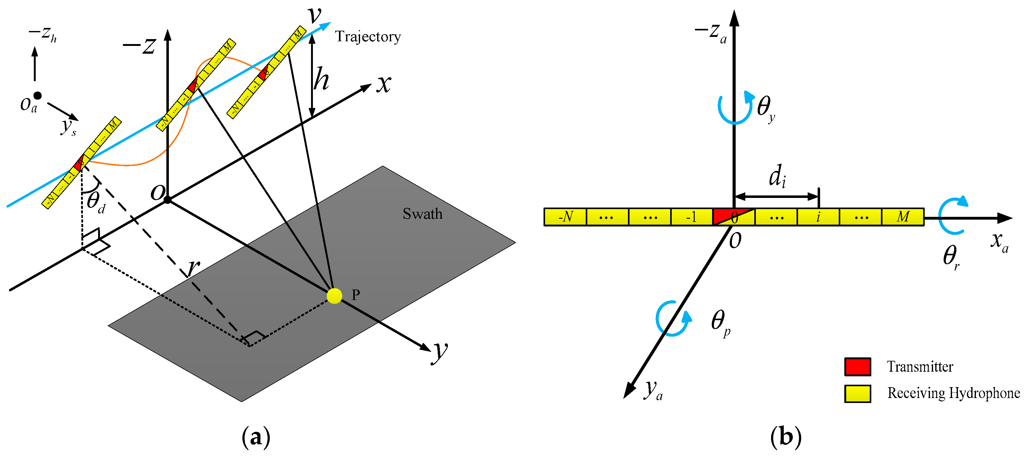
2. Range History Model

2.1. Exact Range History

As shown in Figure 1a, an imaging coordinate system oxyz is established according to the right-hand rule, where the z-axis is pointed upward, and the x-axis and y-axis are in a horizontal plane and perpendicular to each other. An acoustic array, which contains an M + N + 1 hydrophone and one transponder, moves in the oxyz coordinate system. The velocity of the acoustic array along the x-axis is v, and the offsets along the y-axis and z-axis are sway $y_s$ and heave $z_h$, respectively. To describe the gestures of the acoustic array, a moving coordinate system $o{x}_a{y}_a{z}_a$ is built as shown in Figure 1b, where the origin and $x_a$-axis are the phase center of the transponder and the phase center line of the hydrophones, respectively. The roll, pitch, and yaw of the acoustic array are denoted by ${\theta }_r$,${\theta }_p$, and ${\theta }_y$, respectively.

In Figure 1a, when the transponder transmits the signal at position $\left(vt,y_s,-h-z_h\right)$, the distance from the transponder to P$\left(x_0,r\sin {\theta }_d,0\right)$ is as follows:

$$R_T^{*}\left(t;x_0,r\right)=\sqrt{{\left(vt-x_0\right)}^2+{\left(y_s-r\sin {\theta }_d\right)}^2+{\left(h+z_h\right)}^2}$$

(1)

where $t$ is the slow time, h is the height of the array beyond the seafloor, r is the closest distance between the target and trajectory, and ${\theta }_d$ is the depression angle between r and the z-axis.

Owing to the low speed of underwater sound, the moving distance of the SAS between the transmission and reception cannot be ignored. Assuming that ${\tau }_{mi}^{*}$ is the delay between the moment of the ith hydrophone receiving the echo and the moment of the transponder transmitting signal, the position of the ith hydrophone at the receiving moment is given by the following:

$$\left[\begin{array}{c}{x}_i\\ y_i\\ z_i\end{array}\right]=\left[\begin{array}{c}vt+v{\tau }_{mi}^{*}\\ y_s\\ -h-z_h\end{array}\right]+M_r^T\left[\begin{array}{c}{d}_i\\ 0\\ 0\end{array}\right]=\left[\begin{array}{c}v{\tau }_{mi}^{*}+vt+d_i\cos {\theta }_y\cos {\theta }_p\\ y_s-d_i\sin {\theta }_y\cos {\theta }_p\\ -h-z_h-d_i\sin {\theta }_p\end{array}\right],$$

(2)

where $d_i$ is the distance from the ith hydrophone to the transponder and $M_r$ is a rotation matrix given in [14]. According to the location of P and the ith hydrophone at the receiving moment, the distance from P to the ith hydrophone is as follows:

$$\begin{array}{l}{R}_{Ri}^{*}(t;x_0,r)=\sqrt{{(vt+v{\tau }_{mi}^{*}+d_i\cos {\theta }_y\cos {\theta }_p-x_0)}^2}\\ \overline{+{(r\sin {\theta }_d+d_i\sin {\theta }_y\cos {\theta }_p-y_s)}^2+{\left(h+z_h+d_i\sin {\theta }_p\right)}^2}\end{array},$$

(3)

The exact propagation distance of sound from the transmission to reception is the sum of $R_T^{*}\left(t;x_0,r\right)$ and $R_{Ri}^{*}\left(t;x_0,r\right)$, which is expressed as follows:

$$R_{mi}^{*}(t;x_0,r)=R_T^{*}(t;x_0,r)+R_{Ri}^{*}(t;x_0,r).$$

(4)

This is referred to as the exact range history. However, because the echo signal received by the ith hydrophone is propagated for ${\tau }_{mi}^{*}$, the exact range history can be expressed as follows:

$$R_{mi}^{*}(t;x_0,r)=c{\tau }_{mi}^{*},$$

(5)

where c is the speed of underwater sound. By combining (4) and (5), the solution for ${\tau }_{mi}^{*}$ is given as follows:

$${\tau }_{mi}^{*}=\frac{B_{mi}+\sqrt{B_{mi}^2+C_{mi}}}{A},$$

(6)

where A, $B_{mi}$, and $C_{mi}$, respectively, are represented as follows:

$$A=c^2-v^2,$$

(7)

$$B_{mi}=v{d}_i\cos {\theta }_y\cos {\theta }_p+v^2\left(t-\frac{x_0}{v}\right)+c\sqrt{v^2{\left(t-\frac{x_0}{v}\right)}^2+{\left(r\sin {\theta }_d-y_s\right)}^2+{\left(h+z_h\right)}^2},$$

(8)

$$C_{mi}=2v\left(t-\frac{x_0}{v}\right)d_i\cos {\theta }_y\cos {\theta }_p+2\left(h+z_h\right)d_i\sin {\theta }_p+d_i^2+2\left(r\sin {\theta }_d-y_s\right)d_i\sin {\theta }_y\cos {\theta }_p.$$

(9)

2.2. Exact Motion Error

Because yaw and pitch, particularly yaw, can change the direction of the SAS beam and cause the squint phenomenon, we selected the squint model as the ideal model for the multi-hydrophone SAS without loss of generality. Assuming that the mean of yaw and pitch are ${\theta }_{y0}$ and ${\theta }_{p0},$ respectively, the ideal range history is given in [15] and is expressed as follows:

$$R_i^{*}(t;x_0,r)=\frac{B_i+\sqrt{B_i^2+C_i}}{A}c,$$

(10)

where

$$B_i=v{d}_i\cos {\theta }_{y0}\cos {\theta }_{p0}+v^2\left(t-\frac{x_0}{v}\right)+c\sqrt{v^2{\left(t-\frac{x_0}{v}\right)}^2+r^2},$$

(11)

$$C_i=2v\left(t-\frac{x_0}{v}\right)d_i\cos {\theta }_{s0}\cos {\theta }_{p0}+2h{d}_i\sin {\theta }_{p0}+2d_{i}r\sin {\theta }_d\sin {\theta }_{y0}\cos {\theta }_{p0}+d_i^2.$$

(12)

The exact motion error is the difference between the exact range history and the ideal range history and is obtained by subtracting (10) from (5) as follows:

$${\epsilon }_i^{*}(t;x_0,r)=\frac{B_{mi}+\sqrt{B_{mi}^2+A{C}_{mi}}}{A}c-\frac{B_i+\sqrt{B_i^2+A{C}_i}}{A}c,$$

(13)

It can be noted from (13) that this motion error is a 2-D SV and hydrophone-dependent term because its size is related to the target position at the beam and the hydrophone position in the acoustic array.

2.3. Sub-Beam Range History

The SAS echo can be viewed as the sum of all sub-beam echoes, as shown in Figure 2. Assuming that the number of sub-beams is K and the squint angle of the kth sub-beam is ${\theta }_k$, the moment is $x_0/v+r\tan {\theta }_k/v$ when the beam center of the kth sub-beam crosses target P. Because the sub-beam beamwidth is very narrow, the motion error of all targets illuminated by the sub-beam can be replaced by the motion error of the targets at the beam center of the sub-beam. By substituting $t_k$ into (13), the approximation motion error of the kth sub-beam can be obtained as follows:

$${\epsilon }_{i,k}(r)=\frac{B_{mi}^{\prime }+\sqrt{{B_{mi}^{\prime }}^2+A{C}_{mi}^{\prime }}}{A}c-\frac{B_i^{\prime }+\sqrt{{B_i^{\prime }}^2+A{C}_i^{\prime }}}{A}c$$

(14)

where

$$B_{mi}^{\prime }=v{d}_i\cos {\theta }_y\cos {\theta }_p+vr\tan {\theta }_k+c\sqrt{r^2{\tan }^2{\theta }_k+{\left(r\sin {\theta }_d-y_s\right)}^2+{\left(h+z_h\right)}^2},$$

(15)

$$C_{mi}^{\prime }=2d_{i}r\tan {\theta }_k\cos {\theta }_y\cos {\theta }_p+2\left(h+z_h\right)d_i\sin {\theta }_p+d_i^2+2\left(r\sin {\theta }_d-y_s\right)d_i\sin {\theta }_y\cos {\theta }_p,$$

(16)

$$B_i^{\prime }=v{d}_i\cos {\theta }_{y0}\cos {\theta }_{p0}+vr\tan {\theta }_k+c\sqrt{r^2{\tan }^2{\theta }_k+r^2},$$

(17)

$$C_i^{\prime }=2r{d}_i\tan {\theta }_k\cos {\theta }_{s0}\cos {\theta }_{p0}+2h{d}_i\sin {\theta }_{p0}+2r{d}_i\sin {\theta }_d\sin {\theta }_{y0}\cos {\theta }_{p0}+d_i^2.$$

(18)

The range history of the sub-beam can be viewed as the sum of the ideal range history and motion error; thus, the range history of the kth sub-beam can be expressed as follows:

$$R_{mi,k}(t;r)=R_i^{*}(t;r)+{\epsilon }_{i,k}(r).$$

(19)

Considering that the expression of $R_i^{*}\left(t;r\right)$ is very complex, it is necessary to simplify it. According to the description of the displaced phase center antenna (DPCA) technology [16], the multi-hydrophone SAS can be viewed as a monostatic hydrophone transmit signal and receive echo at the phase center of the bistatic transponder/hydrophone pair. Thus, the range history $R_i^{*}\left(t;r\right)$ can be considered as the sum of a single root term and a range-dependent term and is rewritten as follows:

$$R_i^{*}(t;r)=R_i(t;r)+\Delta R_i\left(r\right),$$

(20)

where $R_i\left(t;r\right)$ is the single root term, which is equivalent to the range history of the monostatic hydrophone, and $\Delta R_i\left(r\right)$ is the range-dependent offset term, which is the offset distance attained by transforming a bistatic transponder/hydrophone pair into a monostatic hydrophone. $R_i\left(t;r\right)$ and $\Delta R_i\left(r\right)$ are given as follows:

$$R_i(t;r)=2\sqrt{r^2+v^2{\left(t+\frac{r}{c}+\frac{d_i}{2v\cos {\theta }_{sq0}}\right)}^2},$$

(21)

$$\Delta R_i\left(r\right)=\frac{v^2}{4r}{\left(\frac{2r}{c}+\frac{d_i}{v}\right)}^2-\frac{r}{2}+\frac{{(d_i\sin {\theta }_{p0}+h)}^2}{2r}+\frac{{(d_i\sin {\theta }_{y0}\cos {\theta }_{p0}+r\sin {\theta }_d)}^2}{2r},$$

(22)

where ${\theta }_{sq0}$ is the squint angle.

It can be noted from (22) and (14) that $\Delta R_i\left(r\right)$ and ${\epsilon }_{i,k}\left(r\right)$ are both range-dependent terms; thus, they can be integrated into one term for convenience as expressed below.

$${\zeta }_{i,k}\left(r\right)=\Delta R_i\left(r\right)+{\epsilon }_{i,k}(r),$$

(23)

referred to as the motion compensation term. Then, the range history of the kth sub-beam can be rewritten as follows:

$$R_i^{*}(t;r)=R_i(t;r)+{\zeta }_{i,k}\left(t;r\right).$$

(24)

To evaluate the size of the path error caused by approximating $R_i^{*}\left(t;r\right)$ into $R_{mi,k}\left(t;r\right)$, a simulation was performed. We assume that the acoustic array is shown in Figure 1b, where $N$ and $M$ are equal to 25 and 0, respectively. The system parameters of the SAS are shown in

Table 1. System parameters.

Carrier Frequency (kHz)	80,32,20	Pulse Width (ms)	20	PRF (Hz)	2.5
Bandwidth (kHz)	20	Speed (m/s)	2.5	Hydrophone (m)	0.08
Altitude (m)	30	Transmitter (m)	0.16	Hydrophone number	25

, and the motion parameters are shown in Figure 3, where ${\theta }_y$,${\theta }_p$, $y_s$, and $z_h$ vary randomly with the pulses in $\left[-1^{\circ },1^{\circ }\right]$, $\left[0^{\circ },2^{\circ }\right]$, $\left[-1.5,1.5\right]m$, and $\left[-0.1,0.1\right]m$, respectively. Considering that the beam width is a very important factor in determining the size of the 2-D SV motion error, this simulation was carried out for different beam widths. To compare the results of different beam widths under the same acoustic array and resolution, the SAS beamwidth was changed by adjusting the center frequency of the transmitted signal. Thus, there are three types of center frequencies, as listed in Table 1, whose wavelengths are ${\lambda }_1\left(1.87\mathrm{cm}\right)$, ${\lambda }_2\left(3.75\mathrm{cm}\right)$, and ${\lambda }_3\left(7.5\mathrm{cm}\right)$ with beamwidths of $6^{\circ }$, ${15}^{\circ }$, and ${24}^{\circ }$, respectively.

Without a loss of generality, the hydrophone at the farthest distance from the transponder was selected, and the maxima of ${\theta }_y$,${\theta }_p$, $y_s$, and $z_h$ were used to calculate the motion error. In the proposed method, the total number of sub-beams for beamwidths of $6^{\circ }$, ${15}^{\circ },$ and ${24}^{\circ }$ are 20, 40, and 55, respectively. In the conventional algorithm, the motion errors of all targets illuminated by the SAS beam are replaced by the motion errors of the targets on the center line of the SAS beam. The results of the two algorithms were measured in terms of the wavelength ($\lambda$), as shown in Figure 4.

First, as shown in Figure 4a–c, the beamwidth has a significant influence on the size of the path error in the conventional algorithm. By using the threshold of the path error as 0.0625 (1/16) wavelengths, we measured the maximum path error in Figure 4a–c. The results were $0.3058{\lambda }_1$, $0.5878{\lambda }_2$, and $0.8919{\lambda }_3$, respectively, which are significantly larger than 0.0625 wavelengths. Therefore, it can be concluded that the size of the path error in the conventional algorithm has a significant effect on the imaging results after MOCO.

Next, it can be observed from Figure 4d–f that the beamwidth has little influence on the size of the path error. The main reason for this beneficial result is that the beamwidth of the central sub-beam is sufficiently narrow such that the size of the path error is small when the motion errors of all targets observed by the sub-beam are replaced by the motion errors of the targets at the beam center of the sub-beam. Theoretically, the farther the sub-beam is from the beam center of the SAS, the greater the size of the path error of the sub-beam. Thus, without loss of generality, we selected the sub-beam at the SAS beam edge for analysis. In Figure 4, the images of the second row and the third row are the path error results of the central and edge sub-beams at different beamwidths, respectively. By comparing the images of the two rows, it is clear that the edge sub-beams have a greater path error than the central sub-beams. To evaluate the size of the path error of these sub-beams quantitatively, we measured the maximum path error in Figure 4d–i. The results were $0.0104{\lambda }_1$, $0.0052{\lambda }_2$,$0.0059{\lambda }_3$,$0.0461{\lambda }_1$, $0.0527{\lambda }_2$, and $0.0538{\lambda }_3$, respectively. Although the results show that the path errors of the edge sub-beams are evidently larger than that of the central sub-beams, they are all less than the threshold of 0.0625 wavelengths. Therefore, it can be concluded that the size of the path error in the proposed algorithm has no effect on the imaging result after MOCO.

3. Signal Model

The echo signal of the ith hydrophone can be considered the sum of the echo signals collected by each sub-beam and is expressed as follows:

$$s_i(t,\tau ;r)={\displaystyle \sum _{k=1}^K{s}_{i,k}(t,\tau ;r)}$$

(25)

$s_{i,k}\left(\tau ,t;r\right)$ is the echo signal collected by the kth sub-beam of the ith hydrophone after demodulation and is expressed as follows:

$$\begin{array}{ll}{s}_{i,k}(t,\tau ;r)& =w_r\left(\tau -\frac{R_i(t;r)+{\zeta }_{i,k}\left(t;r\right)}{c}\right){\omega }_a\left(t\right)\exp \left\{-j\frac{2\pi f_0}{c}\left[R_i(t;r)+{\zeta }_{i,k}\left(t;r\right)\right]\right\}\\ & \times \exp \left\{j\pi K_r{\left(\tau -\frac{R_i(t;r)+{\zeta }_{i,k}\left(t;r\right)}{c}\right)}^2\right\}\end{array}$$

(26)

where ${\mathsf{\omega }}_r(\Delta )$ represents the envelope of the transmitted signal, ${\mathsf{\omega }}_{\mathrm{az}}(\Delta )$ represents the beam pattern of a transponder and a hydrophone, $\tau$ is the fast time, $K_{\mathrm{r}}$ is the FM rate of the transmitted signal, and $f_0$ is the center frequency of the transmitted signal.

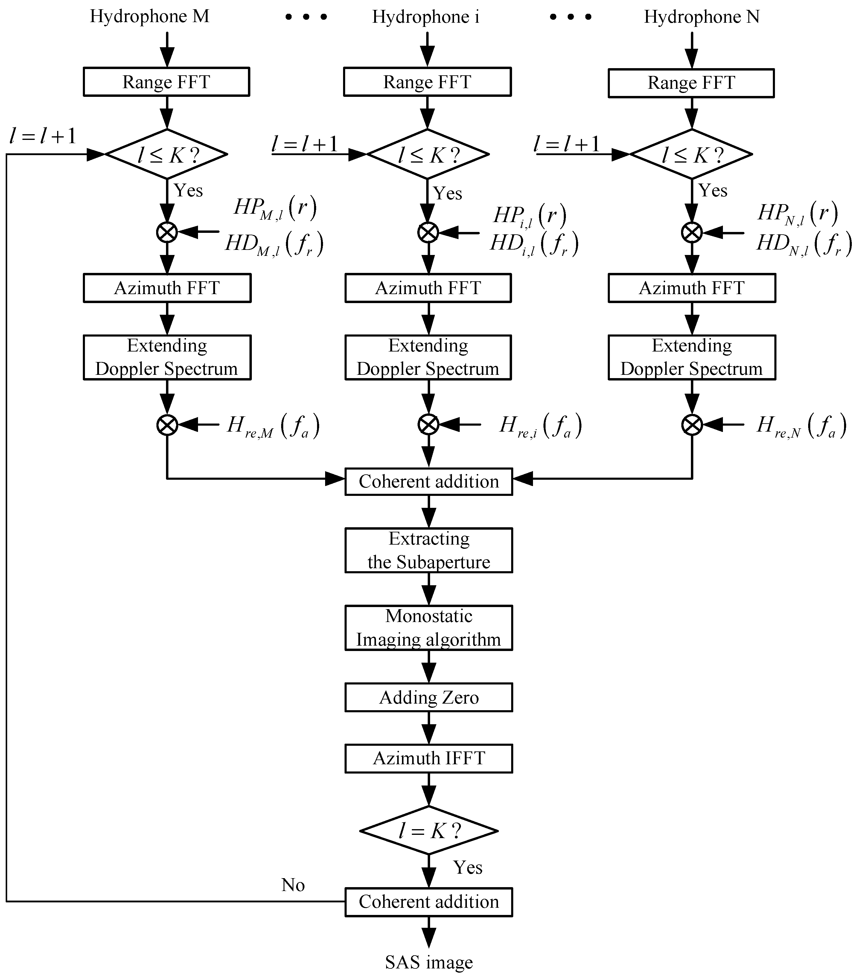
4. Development of the Motion Compensation

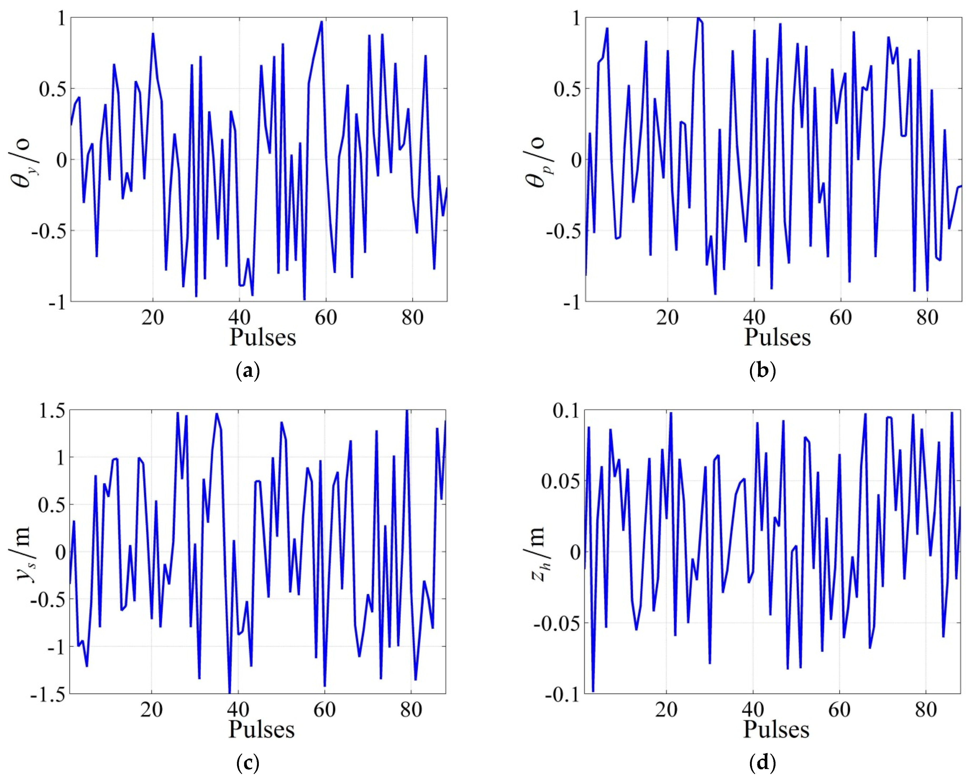
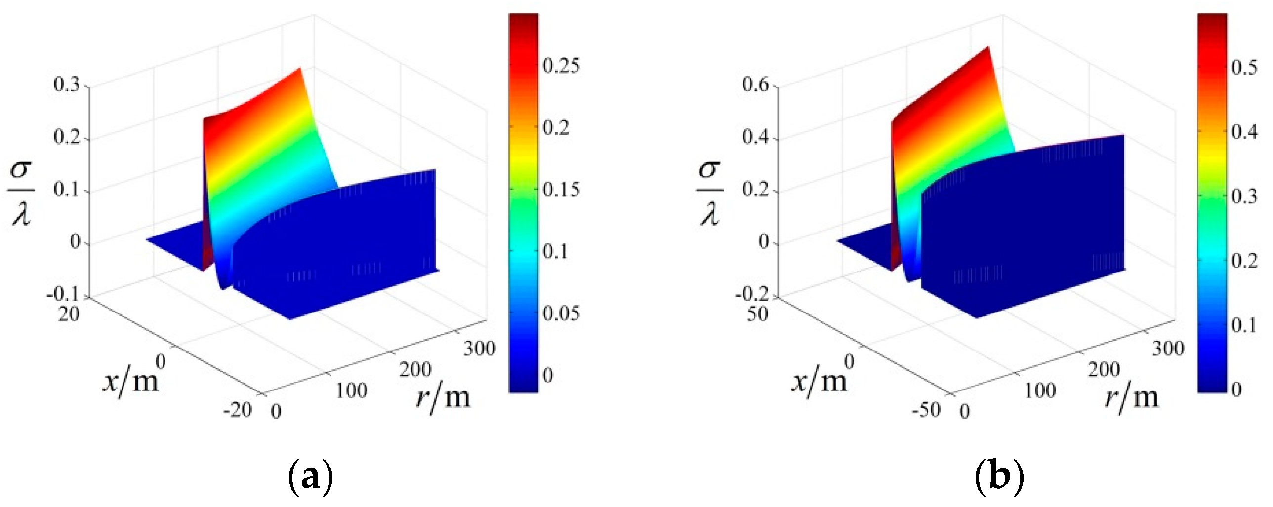
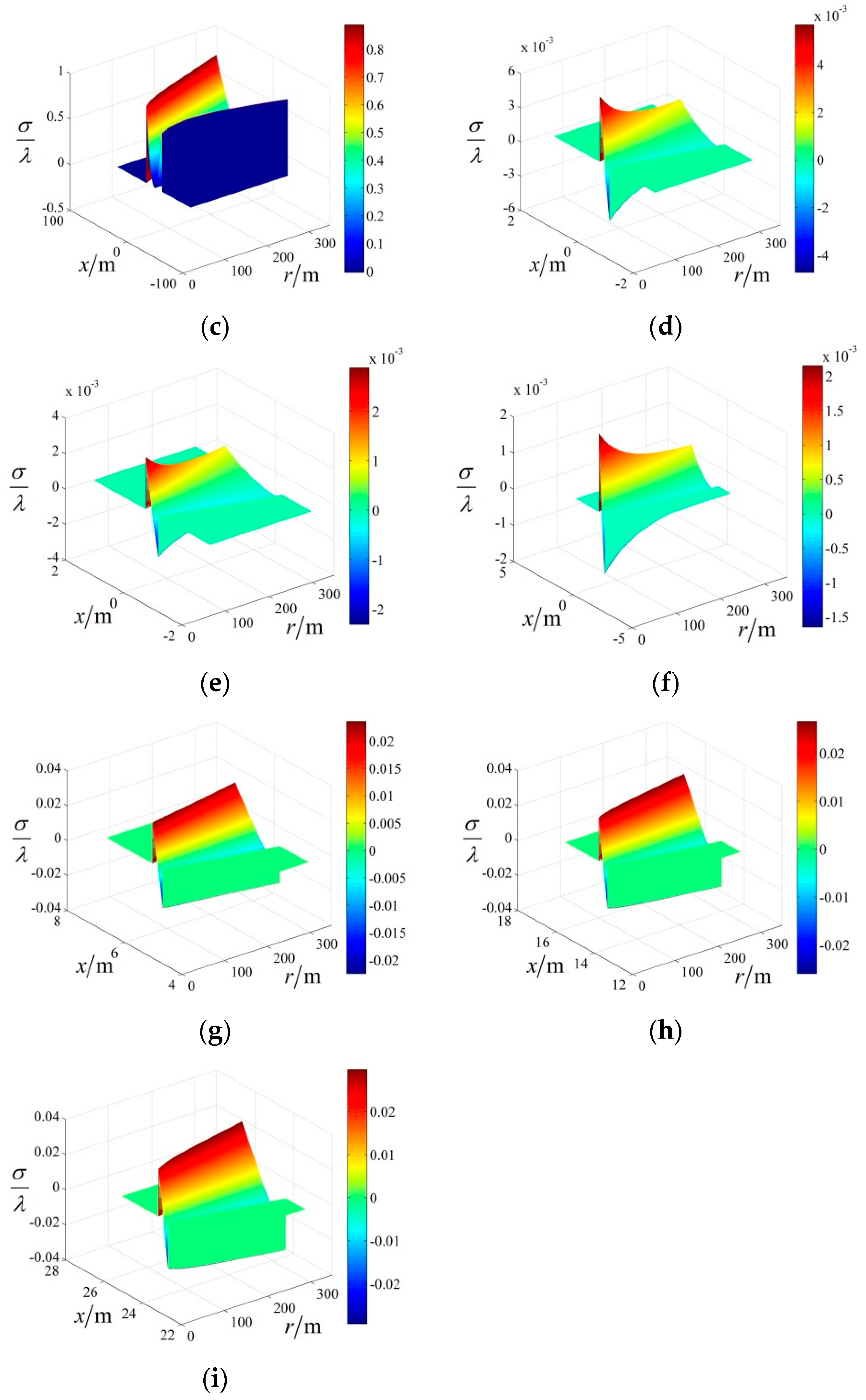
The proposed algorithm contains the range Fourier transformation, phase and delay correction for the sub-beam, azimuth Fourier transformation, azimuth spectrum replication, coherent addition for each hydrophone, Doppler spectrum division, monostatic imaging, azimuth inverse Fourier transformation, and coherent addition for the imaging result of each sub-beam, as shown in Figure 5.

The first step is to transform $s_i\left(\tau ,t;r\right)$ into the range frequency domain. Here, the principle of the stationary phase (POSP) [17] is used to perform the range Fourier transformation on $s_i\left(\tau ,t;r\right)$. The results of the range Fourier transformation are as follows:

$$\begin{array}{ll}{S}_i(f_r,t;r)& =A_0{W}_r\left(f_r\right){\omega }_a\left(t\right)\exp \left(-j\frac{\pi f_r^2}{K_r}\right)\exp \left[-j2\pi \frac{R_i(t;r)}{c}\left(f_0+f_r\right)\right]\\ & \times {\displaystyle \sum _{k=1}^K\left\{\exp \left[-j2\pi \frac{{\zeta }_{i,k}\left(r\right)}{c}{f}_0\right]\times \exp \left[-j2\pi \frac{{\zeta }_{i,k}\left(r\right)}{c}{f}_r\right]\right\}}\end{array}$$

(27)

where $W_r(.)$ represents the spectral envelope of the transmitted signal, and $f_r$ is the range frequency.

The second step is to compensate for the sub-beam motion error by the phase correction and delay correction in the order of one-by-one hydrophone. The phase correction is performed on $S_i\left(f_r,t;r\right)$ with phase multiplication, where the factor for the phase multiplication is given by the following:

$$H{P}_{i,l}\left(r\right)=\exp \left[j\frac{2\pi f_0}{c}{\zeta }_{i,l}\left(r\right)\right]$$

(28)

where the subscript l represents the lth sub-beam. Because ${\xi }_{i,l}\left(t;r\right)$ is weakly dependent on the range, the delay caused by ${\xi }_{i,l}\left(t;r\right)$ can be considered the same as the delay along the range, which can be replaced by the delay at reference range. According to the Fourier transform shifting properties, the constant delay can be corrected by performing a phase multiplication on $S_i\left(f_r,t;r\right)$, where the factor for this phase multiplication is given as follows:

$$H{D}_{i,l}\left(t;f_r\right)=\exp \left[j\frac{2\pi f_r}{c}{\zeta }_{i,l}\left(r_{ref}\right)\right]$$

(29)

After multiplying (27) with (28) and (29) separately, the signal of the ith hydrophone is expressed as follows:

$$\begin{array}{ll}{S}_{i,l}(f_r,t;r)& =A_0{W}_r\left(f_r\right){\omega }_a\left(t\right)\exp \left(-j\frac{\pi f_r^2}{K_r}\right)\exp \left[-j2\pi \frac{R_i(t;r)}{c}\left(f_0+f_r\right)\right]\\ & \times {\displaystyle \sum _{k=1}^K\left\{\exp \left[-j2\pi \frac{{\zeta }_{i,k}\left(r\right)-{\zeta }_{i,l}\left(r\right)}{c}{f}_0\right]\times \exp \left[-j2\pi \frac{{\zeta }_{i,k}\left(r\right)-{\zeta }_{i,l}\left(r_{ref}\right)}{c}{f}_r\right]\right\}}\end{array}$$

(30)

The third step is the azimuth Fourier transformation. Here, we again utilize the POSP to perform the azimuth Fourier transform on $S_{i,l}\left(f_r,t;r\right)$. The results of the range Fourier transform are as follows:

$$\begin{array}{ll}{S}_{i,l}(f_r,f_a;r)& =A_0{W}_r\left(\frac{f_r}{K_r}\right)W_a\left(f_a\right)\exp \left(-j\frac{\pi f_r^2}{K_r}\right)\exp \left(-j\frac{4\pi r{f}_0}{c}\sqrt{\frac{f_r^2}{f_0^2}+\frac{2f_r}{f_0}+D^2}\right)\\ & \times \exp \left(-j\frac{2\pi r{f}_a}{c}\right)\exp \left(-j\frac{2\pi d_i{f}_a}{2v\cos {\theta }_{sq0}}\right)\\ & \times {\displaystyle \sum _{k=1}^K\left\{\exp \left[-j2\pi \frac{{\zeta }_{i,k}\left(r\right)-{\zeta }_{i,l}\left(r\right)}{c}{f}_0\right]\times \exp \left[-j2\pi \frac{{\zeta }_{i,k}\left(r\right)-{\zeta }_{i,l}\left(r_{ref}\right)}{c}{f}_r\right]\right\}}\end{array}$$

(31)

where D is the range migration factor and is represented as follows:

$$D=\sqrt{1-\frac{c^2{f}_a^2}{4v^2{f}_0^2}}$$

(32)

The fourth step is the azimuth spectrum replication. The 2-D spectrum of each hydrophone in (31) suffers a serious problem of azimuth undersampling owing to the principle of multi-hydrophone SAS. Thus, it becomes difficult for the multi-hydrophone SAS to obtain a 2-D spectrum without azimuth aliasing before extracting the 2-D spectrum of the sub-beam from (31). The method of azimuth spectrum replication was proposed to solve this problem. This method includes two main steps. The first step is to replicate the undersampled 2-D spectrum of each hydrophone $N+M+1$ times. The second step is to rank the replicated 2-D spectrum end-to-end in azimuth. Although the method of azimuth spectrum replication cannot suppress azimuth aliasing, it provides an effective method to deal with the undersampled 2-D spectrum in azimuth.

The fifth step is to coherently add the signal of each hydrophone. To remove the azimuth aliasing caused by the azimuth undersampling of each hydrophone, a method that coherently adds the corrected signal of each hydrophone is utilized as follows:

$$S_l(f_r,f_a;r)=\left[\begin{array}{ccccc}{H}_{re,N}\left(f_a\right)& \cdots & H_{re,i}\left(f_a\right)& \cdots & H_{re,M}\left(f_a\right)\end{array}\right]\left[\begin{array}{c}{S}_{N,l}(f_r,f_a;r)\\ ⋮\\ S_{i,l}(f_r,f_a;r)\\ ⋮\\ S_{M,l}(f_r,f_a;r)\end{array}\right]$$

(33)

where

$$H_{re,i}\left(f_a\right)=\exp \left(j\frac{\pi d_i{f}_a}{v\cos {\theta }_{sq0}}\right)$$

(34)

The result is given as follows:

$$\begin{array}{ll}{S}_l(f_r,f_a;r)& =A_0{W}_r\left(\frac{f_r}{K_r}\right)W_a\left(f_a\right)\exp \left(-j\frac{\pi f_r^2}{K_r}\right)\\ & \times \exp \left(-j\frac{2\pi r{f}_a}{c}\right)\exp \left(-j\frac{4\pi r{f}_0}{c}\sqrt{\frac{f_r^2}{f_0^2}+\frac{2f_r}{f_0}+D^2}\right)\\ & \times \{\begin{array}{l}1,f_{a,l}-\frac{B_{a,l}}{2}\le f_a\le f_{a,l}+\frac{B_{a,l}}{2}\\ {\displaystyle \sum _{i=N}^M{\displaystyle \sum _{k=1,k\ne l}^K\left\{\begin{array}{l}\exp \left[-j2\pi \frac{{\zeta }_{i,k}\left(r\right)-{\zeta }_{i,l}\left(r\right)}{c}{f}_0\right]\\ \times \exp \left[-j2\pi \frac{{\zeta }_{i,k}\left(r\right)-{\zeta }_{i,l}\left(r_{ref}\right)}{c}{f}_r\right]\end{array}\right\},else}}\end{array}\end{array}$$

(35)

where $B_{a,l}$ and $f_{a,l}$ define the Doppler bandwidth and Doppler center frequency of the $l^{th}$ sub-beam, respectively. From (35), we can see that only the motion error corresponding to the lth sub-beam is effectively compensated.

The sixth step is to extract the sub-beam’s signal from the 2-D spectrum of the SAS. $B_{a,l}$ and $f_{a,l}$ of the lth sub-beam are calculated by utilizing the mapping relationship between the azimuth view angle and Doppler frequency. According to the values of $B_{a,l}$ and $f_{a,l}$, the signal of the lth sub-beam can be obtained from (35) and is extracted as follows.

$$\begin{array}{ll}{S}_l(f_r,f_a;r)& =A_0{W}_r\left(\frac{f_r}{K_r}\right)W_a\left(f_a\right)\\ & \times \exp \left(-j\frac{\pi f_r^2}{K_r}\right)\exp \left(-j\frac{2\pi r{f}_a}{c}\right)\\ & \times \exp \left(-j\frac{4\pi r{f}_0}{c}\sqrt{\frac{f_r^2}{f_0^2}+\frac{2f_r}{f_0}+D^2}\right),f_{a,l}-\frac{B_{a,l}}{2}\le f_a\le f_{a,l}+\frac{B_{a,l}}{2}\end{array}$$

(36)

The seventh step is to perform the imaging algorithm on the sub-beam signal. The fifth step is essentially a process in which a multi-hydrophone signal is transformed into a monostatic signal; thus, all monostatic imaging algorithms, such as the range–Doppler algorithm [18], chirp scaling algorithm [19], $\omega K$ algorithm ($\omega \mathrm{KA}$) [20], and their modifications, can be performed on the sub-beam signal to obtain the imaging result of each sub-beam. The imaging algorithm mainly includes range cell migration correction, range compression, second range compression, azimuth matched filter, and azimuth inverse Fourier transformation. However, to meet the pixel points for the scene, the data in (36) must be padded with zero in the azimuth before the azimuth inverse Fourier transformation. In addition, to obtain the imaging results of the other sub-beams except for the lth sub-beam, steps 2 to 7 need to be executed repeatedly.

The eighth step is to coherently add the imaging results of all the sub-beams. Because the sub-beam’s Doppler bandwidth is narrow, its imaging result has low resolution. To obtain a high-resolution imaging result, it is necessary to coherently add every sub-beam’s imaging result.

5. Validation Test

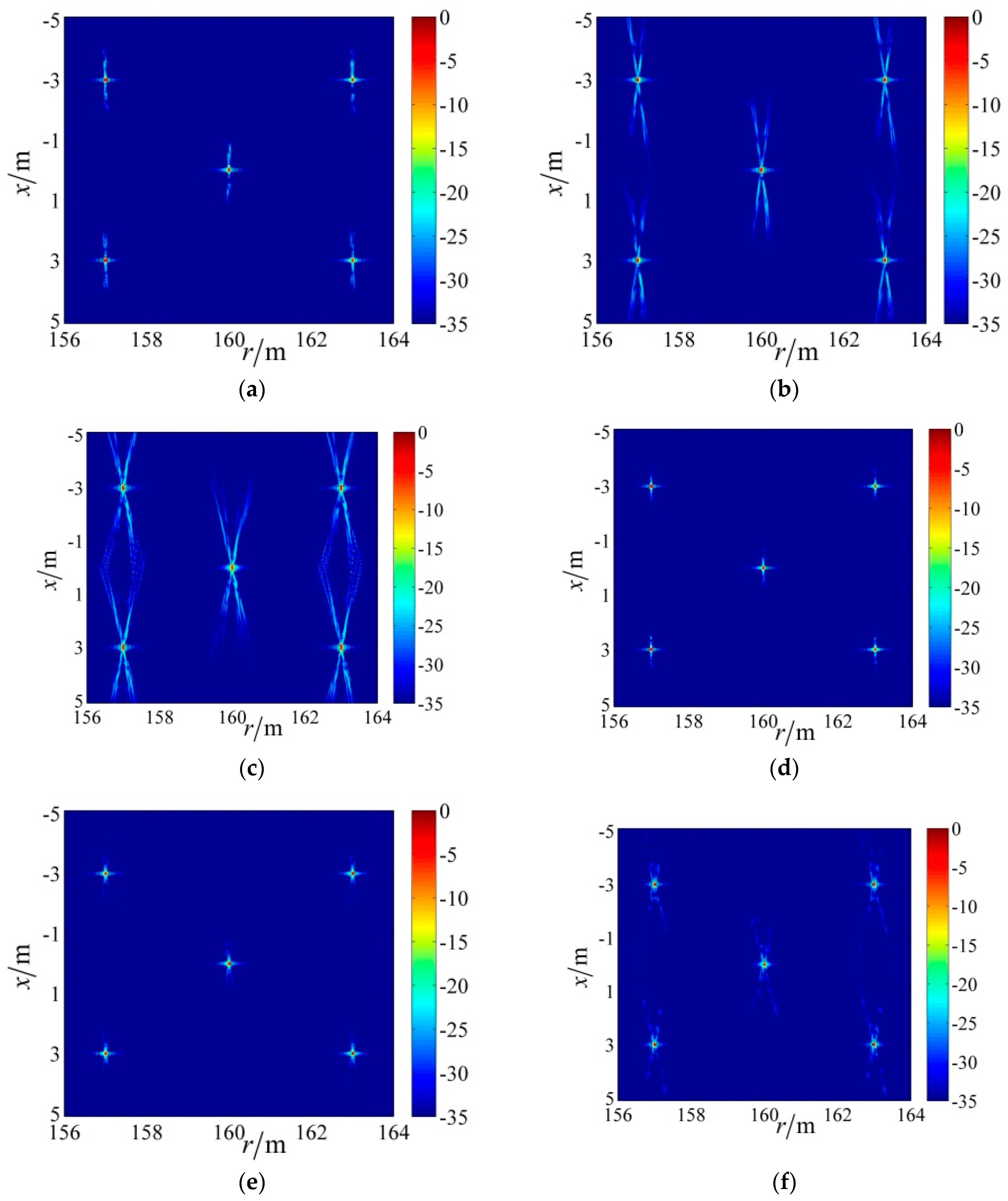
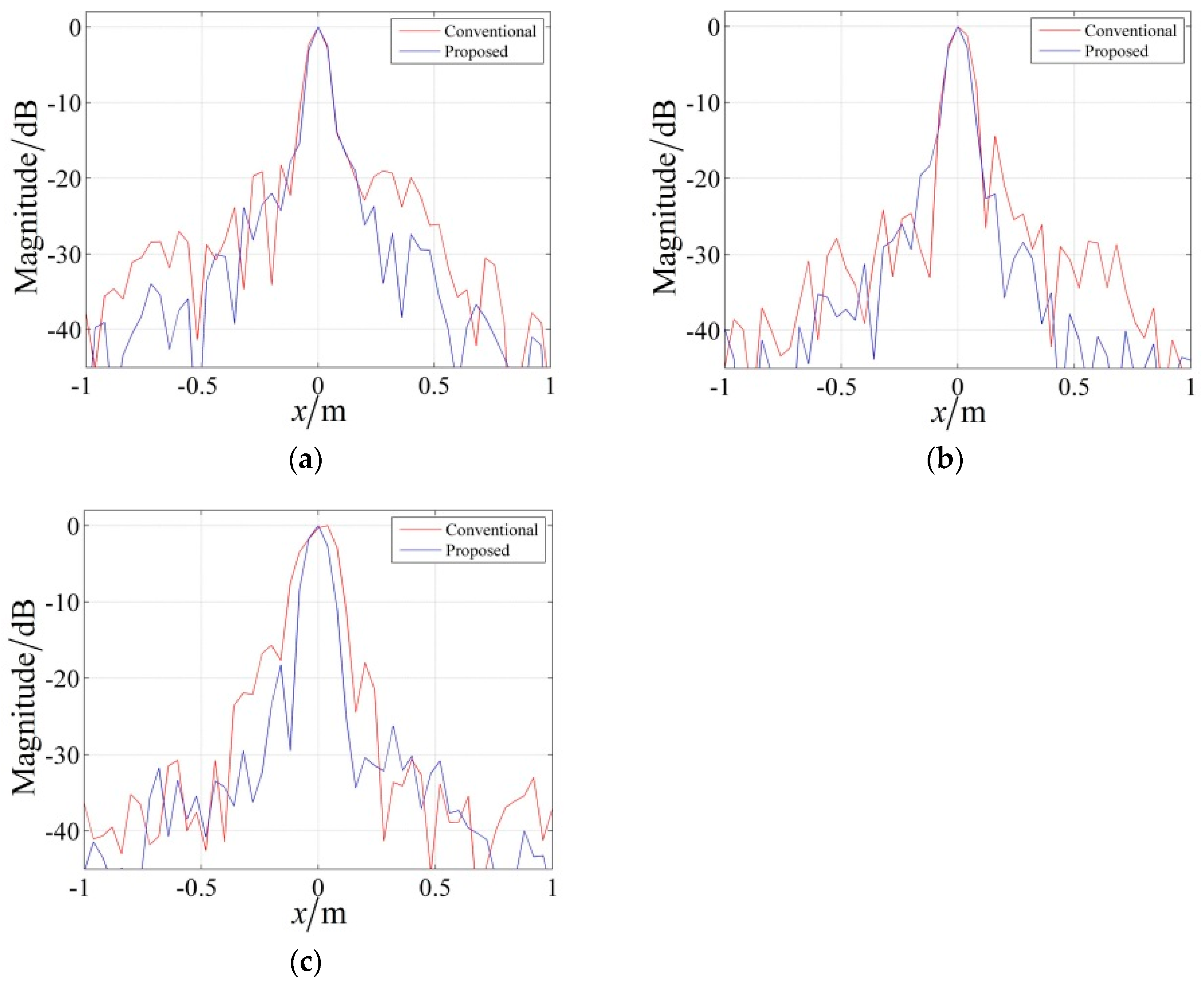
5.1. Exact Range History Imaging Results of Simulation Data

To evaluate the performance of the proposed MOCO algorithm, a simulation was performed. The system parameters are shown in Table 1, the SAS motion error is shown in Figure 3, and the scene illuminated by sonar has five idea point targets, which are assumed to be located at positions P1 (−3 m, 152 m, 30 m), P2 (−3 m, 158 m, 30 m), P3 (3 m, 158 m, 30 m), P4 (3 m, 152 m, 30 m), and P5 (0 m, 155 m, 30 m), respectively. In the simulation, the exact range history of each target is given by (6), and to avoid the new path error caused by the imaging algorithm, a $\omega \mathrm{KA}$ is utilized as the monostatic imaging algorithm in the seventh step. The results of the proposed algorithm and the conventional algorithm are shown in Figure 6.

From Figure 6a–c, it can be observed that the sidelobe energy and azimuth mainlobe width of the imaging results of the conventional algorithm become stronger and wider with the increase in beam width, respectively. Although the imaging results of the proposed algorithm have problems similar to those of the conventional algorithm, the increasing extent of sidelobe level and mainlobe width are less than those of the conventional algorithm, as shown in Figure 6d–f. Next, to compare the imaging results in more detail, point P5 was extracted from the subfigures of Figure 6. Theoretically, the range image is obtained using match filter technology, and the motion has a smaller effect on the range image than the azimuth image. Thus, for convenience, we only made the azimuth slice of point P5, as shown in Figure 7. Then, the impulse response width was measured and compared with the theoretical resolution of 8 cm. From

Table 2. The imaging quality of the results of the conventional algorithm and the proposed algorithm.

Algorithm	Beamwidth	IRW/cm	PSLR/dB	ISLR/dB
The conventional algorithm	6°	8.71	−17.80	−11.32
The proposed algorithm	6°	8.10	−18.05	−14.05
The conventional algorithm	15°	9.99	−14.80	−9.08
The proposed algorithm	15°	8.29	−19.89	−13.62
The conventional algorithm	24°	14.98	−16.01	−7.95
The proposed algorithm	24°	8.94	−18.93	−11.64

, it can be observed from the comparison results that when the beam width is 6°, 15°, and 24°, the mainlobe broadening of the conventional algorithms is 8.9%, 24.9%, and 87.3% at beamwidths of 6°, 15°, and 24°, respectively, while the mainlobe broadening of the proposed algorithm is only 1.2%, 3.6%, and 11.8%. These results show that the imaging result of the proposed algorithm is better than that of the conventional algorithm and is close to the theoretical result. Therefore, the validity of the proposed algorithm was tested through simulation.

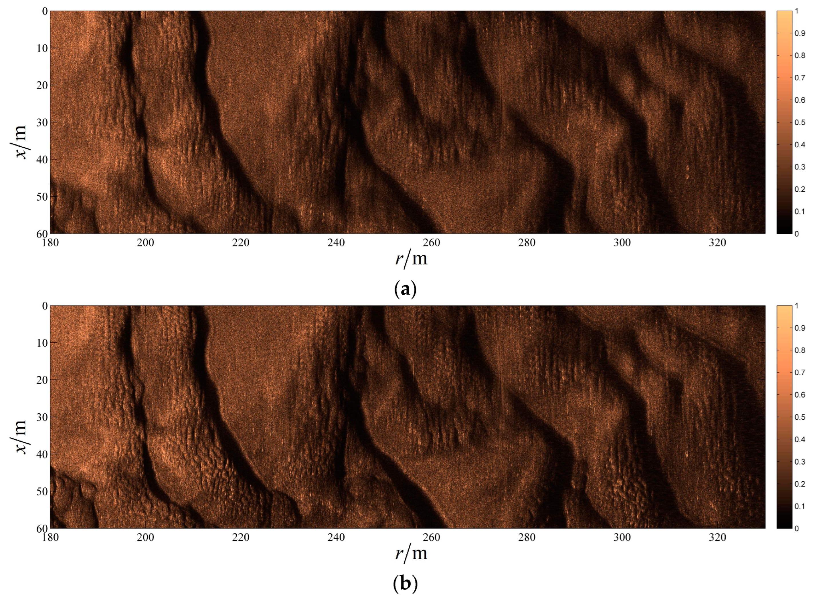
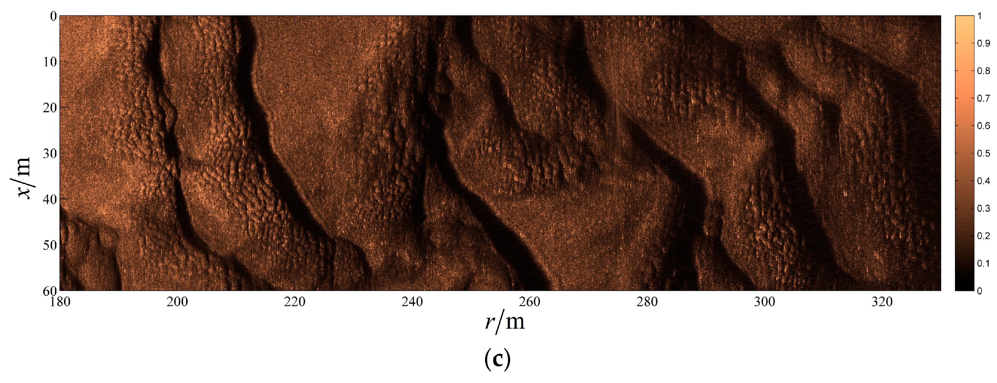
5.2. Imaging Results of Real Data

In this section, the performance of the proposed algorithm is evaluated by comparing the imaging results of different algorithms. The real data were sourced from the South China Sea and were collected using a multi-hydrophone SAS in 2017. The imaging results with no motion compensation, the conventional algorithm, and the proposed algorithm are shown in Figure 8a–c, respectively, where the number of sub-beams in the proposed algorithm is seven.

It can be observed that the image in Figure 8b is clearer and shows more detailed information than the image in Figure 8a; thus, the existing algorithm is effective. However, the image result of the far scene in Figure 8b is worse than that of the near scene. This result indicates that there is still a large path error that is not compensated for by the conventional algorithm. By comparing Figure 8b with Figure 8c, it can be seen that the image result in Figure 8c is better than that in Figure 8b, both in the far scene and in the near scene. Therefore, the validity and superiority of the proposed algorithm are verified.

6. Conclusions

A 2-D SV motion compensation algorithm for a multi-hydrophone SAS based on sub-beam compensation was proposed in this study. To the best of our knowledge, such an algorithm had not yet been reported. The main contributions of this study are as follows: (1) An exact motion error model for the multi-hydrophone SAS, which includes five degrees of freedom, namely roll, pitch, yaw, sway, and heave, is newly established. (2) The ability of the proposed algorithm to compensate for the 2-D SV motion error with hydrophone dependency for the multi-hydrophone SAS is demonstrated. (3) The ability of the proposed algorithm to compensate for low-frequency and high-frequency motion errors simultaneously is also shown. Moreover, the algorithm can be applied to multi-channel SARs, such as the spaceborne SAR. However, the premise of the proposed algorithm is to determine the motion parameters of the platform measured.

References

1. Hayes, M.P.; Gough, P.T. Synthetic Aperture Sonar: A Review of Current Status. IEEE J. Ocean. Eng. 2009, 34, 207–224. [Google Scholar] [CrossRef]
2. Zhang, X.; Wu, H.; Sun, H.; Ying, W. Multireceiver SAS imagery based on monostatic conversion. IEEE J. Sel. Top. Appl. Earth Obs. Remote Sens. 2021, 14, 10835. [Google Scholar] [CrossRef]
3. Zhang, X. An efficient method for the simulation of multireceiver SAS raw signal. Multimed. Tools Appl. 2023, 83, 37351–37368. [Google Scholar] [CrossRef]
4. Scott, B.T.; Brett, B.; Sowmya, R.; Ethan, L.; Bradley, M.; Patrick, R. Environmentally adaptive automated recognition of underwater mines with synthetic aperture sonar imagery. J. Acoust. Soc. Am. 2021, 150, 851–863. [Google Scholar]
5. Angeliki, X.; Yan, P. Compressive synthetic aperture sonar imaging with distributed optimization. J. Acoust. Soc. Am. 2019, 146, 1839–1850. [Google Scholar]
6. Nadimi, N.; Javidan, R.; Layeghi, K. An Efficient Acoustic Scattering Model Based on Target Surface Statistical Descriptors for Synthetic Aperture Sonar Systems. J. Mar. Sci. Appl. 2020, 19, 494–507. [Google Scholar] [CrossRef]
7. Piper, J.E.; Lim, R.; Thorsos, E.I.; Williams, K.L. Buried Sphere Detection Using a Synthetic Aperture Sonar. IEEE J. Ocean. Eng. 2009, 34, 485–494. [Google Scholar] [CrossRef]
8. Callow, H.J. Signal Processing for Synthetic Aperture Sonar Image Enhancement. Ph.D. Thesis, Electrical and Electronic Engineering, University of Canterbury, Christchurch, New Zealand, 2003. [Google Scholar]
9. Macedo, K.A.C.d.; Scheiber, R. Precise topography- and aperture-dependent motion compensation for airborne SAR. IEEE Geosci. Remote Sens. Lett. 2005, 2, 172–176. [Google Scholar]
10. Prats, P.; Reigber, A.; Mallorqui, J.J. Topography-dependent motion compensation for repeat-pass interferometric SAR systems. IEEE Geosci. Remote Sens. Lett. 2005, 2, 206–210. [Google Scholar] [CrossRef]
11. Zheng, X.; Yu, W.; Li, Z. A Novel Algorithm for Wide Beam SAR Motion Compensation Based on Frequency Division. In Proceedings of the 2006 IEEE International Symposium on Geoscience and Remote Sensing, Denver, CO, USA, 31 July–4 August 2006; pp. 3160–3163. [Google Scholar]
12. Lu, Q.; Huang, P.; Gao, Y.; Liu, X. Precise frequency division algorithm for residual aperture-variant motion compensation in synthetic aperture radar. Electron. Lett. 2019, 55, 51–53. [Google Scholar] [CrossRef]
13. Lu, Q.; Gao, Y.; Huang, P.; Liu, X. Range- and Aperture-Dependent Motion Compensation Based on Precise Frequency Division and Chirp Scaling for Synthetic Aperture Radar. IEEE Sens. J. 2019, 19, 1435–1442. [Google Scholar] [CrossRef]
14. Wu, H.; Tang, J.; Zhong, H. A moderate squint imaging algorithm for the multiple-hydrophone SAS with receiving hydrophone dependence. IET Radar Sonar Navig. 2019, 13, 139–147. [Google Scholar] [CrossRef]
15. Wu, H.; Tang, J.; Zhong, H. A Correction Approach for the Inclined Array of Hydrophones in Synthetic Aperture. Sensors 2018, 18, 2000. [Google Scholar] [CrossRef] [PubMed]
16. Zhang, X.; Ying, W.; Dai, X. High-resolution imaging for the multireceiver SAS. J. Eng. 2019, 2019, 6057–6062. [Google Scholar] [CrossRef]
17. Cumming, I.G.; Wong, F.H. Digital Processing of Synthetic Aperture Radar Data: Algorithms and Implementation; Artech House: Norwood, MA, USA, 2005. [Google Scholar]
18. Zhang, X.; Yang, P.; Wang, Y. A Novel Multireceiver SAS RD Processor. IEEE Trans. Geosci. Remote Sens. 2023, 62, 4203611. [Google Scholar] [CrossRef]
19. Zhang, X.; Yang, P.; Wang, Y. LBF-based CS algorithm for multireceiver SAS. IEEE Geosci. Remote Sens. Lett. 2024, 21, 1502505. [Google Scholar] [CrossRef]
20. Cafforio, C.; Prati, C.; Rocca, F. SAR data focusing using seismic migration techniques. IEEE Trans. Aerosp. Electron. Syst. 1991, 27, 194–207. [Google Scholar] [CrossRef]
Figure 1. Geometric model of the multi-hydrophone SAS. (a) Model of range history; (b) array of hydrophones.
Remotesensing 16 02144 g001
Figure 2. Relationship between the Doppler frequency and sub-beam.
Remotesensing 16 02144 g002
Figure 3. Motion error: (a) θ y ; (b) θ p ; (c) y s ; (d) z h .
Remotesensing 16 02144 g003
Figure 4. (ac) are the path error results caused by the conventional algorithm for the beamwidths of 6 , 15 , and 24 , respectively; (df) are the path error results of the central sub-beam caused by the proposed algorithm for the beamwidths of 6 , 15 , and 24 , respectively; (gi) are the path error results of the edge sub-beam caused by the proposed algorithm for the beamwidths of 6 ,   15 , and 24 , respectively.
Remotesensing 16 02144 g004aRemotesensing 16 02144 g004b
Figure 5. Flow chart combining the proposed algorithm.
Remotesensing 16 02144 g005
Figure 6. Imaging results of the conventional algorithm and the proposed algorithm at the different beamwidths. Conventional algorithm: (a) 6 , (b) 15 , and (c) 24 ; Proposed algorithm: (d) 6 , (e) 15 , and (f) 24 .
Remotesensing 16 02144 g006
Figure 7. Azimuth slice of the imaging results of the conventional algorithm and the proposed algorithm at the different beamwidths. (a) 6 , (b) 15 , and (c) 24 .
Remotesensing 16 02144 g007
Figure 8. The imaging results. (a) No motion compensation; (b) the conventional algorithm; (c) the proposed algorithm.
Remotesensing 16 02144 g008aRemotesensing 16 02144 g008b