
A Steering-Vector-Based Matrix Information Geometry Method for Space–Time Adaptive Detection in Heterogeneous Environments

Abstract
:1. Introduction
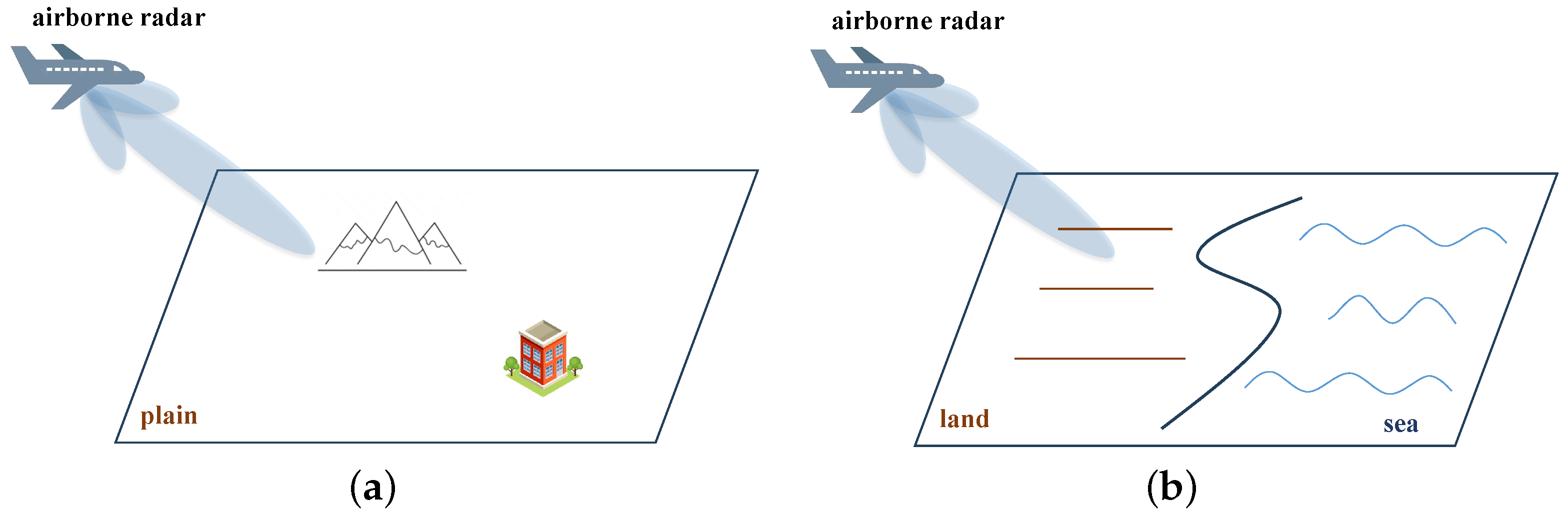
- The given steering vector of the target is abandoned by existing MIG detectors, causing underutilized information in STAD. In addition, the MIG detector fails to suppress the clutter in the spatial and temporal domains; therefore, the performance of the MIG detector can be further improved for airborne radar.
- The various existing MIG detectors are designed for single-channel radar. For multi-channel radar, there is a strong correlation between channels, which has not been considered before. This problem is especially accentuated when the dimensionality of the data matrix increases. At present, MIG detectors can only work with dimensionality reduction algorithms, which put a price on performance loss.
- We provide a novel MIG detector for STAD. The proposed steering-vector-based matrix information (S-MIG) detector introduces the steering vector into target detection, overcoming the shortcomings of the MIG detector and making it feasible to apply information geometry methods to STAD.
- We perform a detailed analysis and validation of the performance of the S-MIG detector, especially the important property that matters in target detection. The mathematical derivation and experimental results illustrate that the proposed S-MIG detector has competitive performance, while its computational burden is comparable to existing methods.
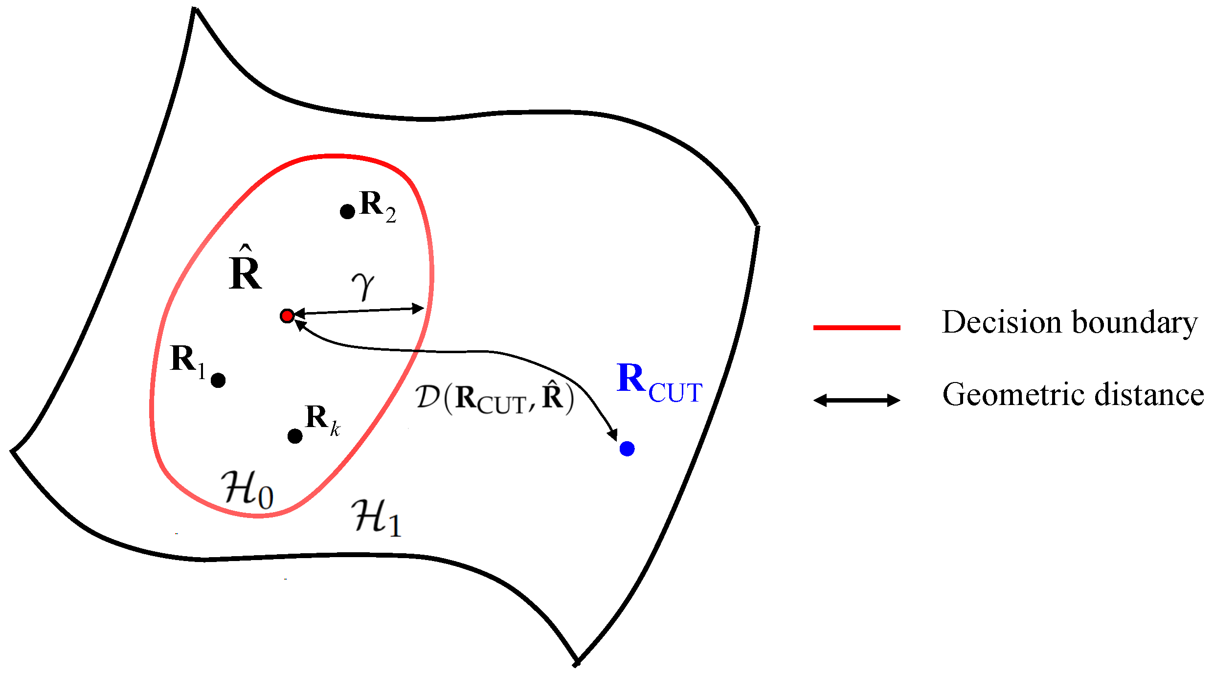
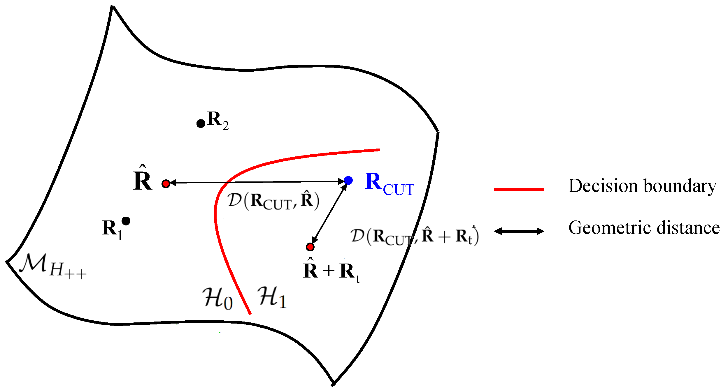
- We describe a novel detection scheme for detectors based on matrix information geometry. In cases for which the target’s steering vector is given, a detection scheme that is a hyperbola on the Hermitian positive definite (HPD) manifold is proposed, and many detection methods based on various metrics can be extended from it.
2. Problem Formulation and Preliminaries of MIG
2.1. Signal Model and Detection Model
2.2. Preliminaries of Matrix Information Geometry
3. Steering-Vector-Based Matrix Information Geometry Detector and Its Performance Analysis
3.1. Steering-Vector-Based Matrix Information Geometry Detector
3.2. Geometric Explanation of the S-MIG Detector
3.3. Performance Analysis
3.3.1. Computation Complexity Analysis
3.3.2. Robustness Analysis
4. Experimental Results and Analysis
4.1. Experiments Based on Simulated Data
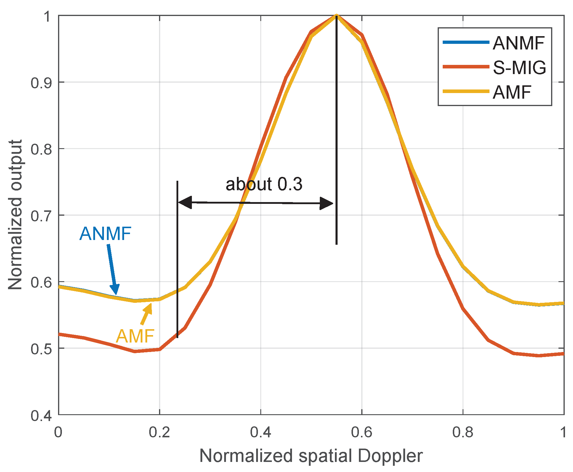
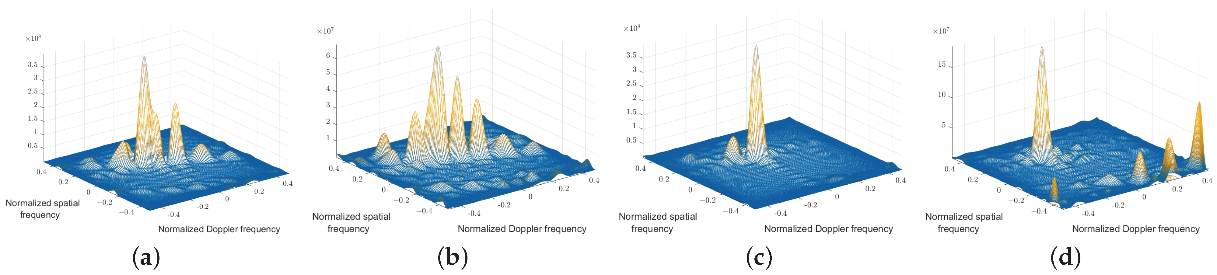
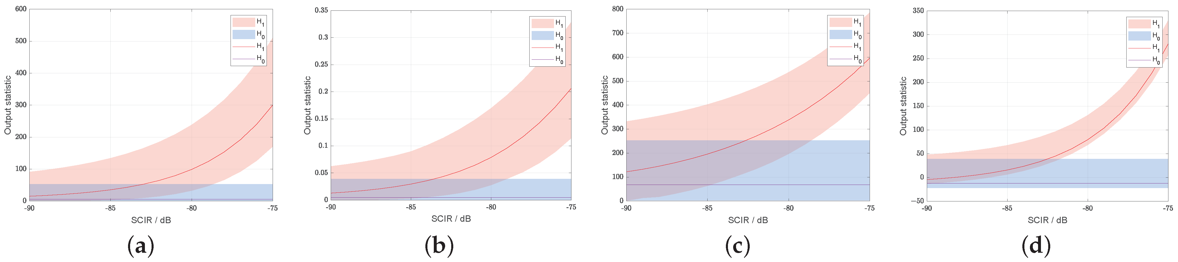
4.1.1. Directional Sensitivity
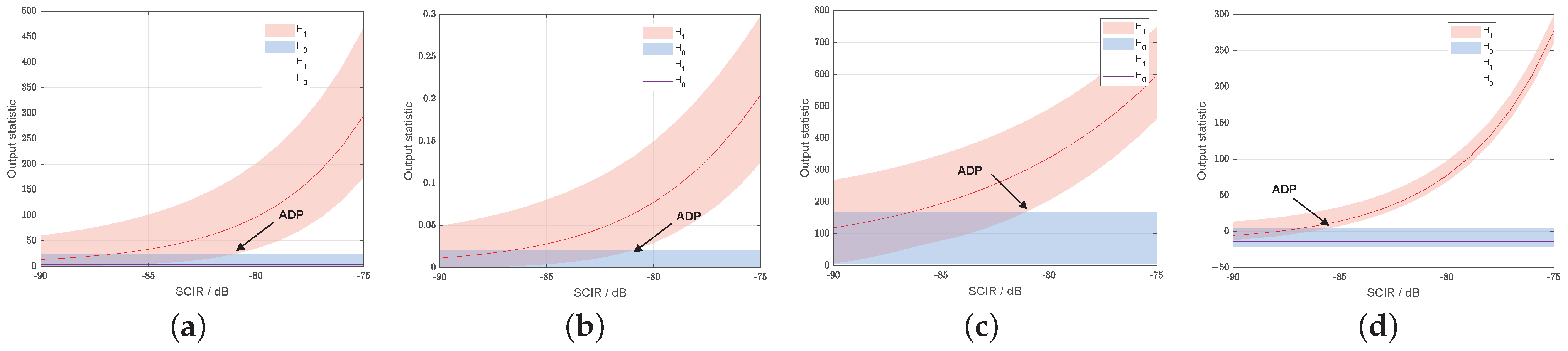
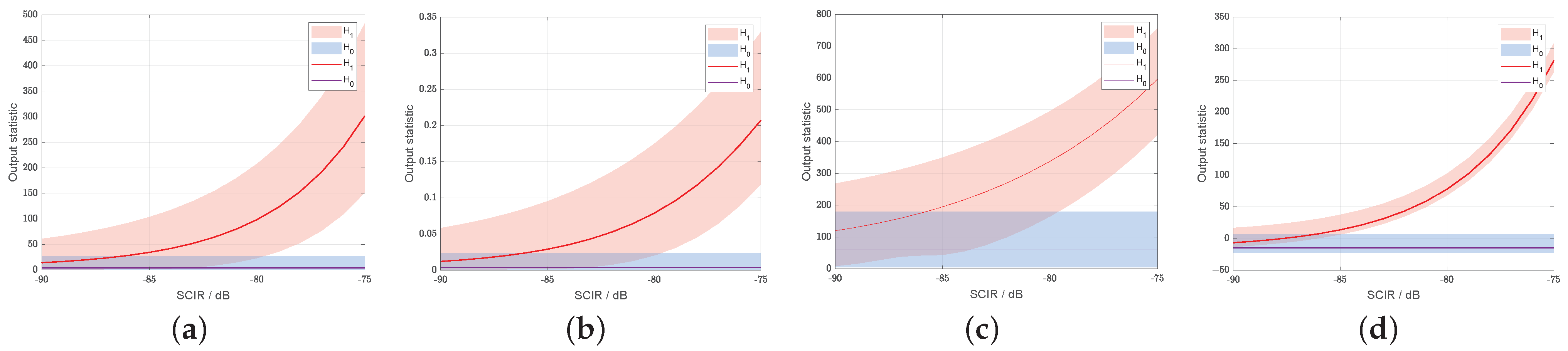
4.1.2. Robustness
4.1.3. Computational Efficiency
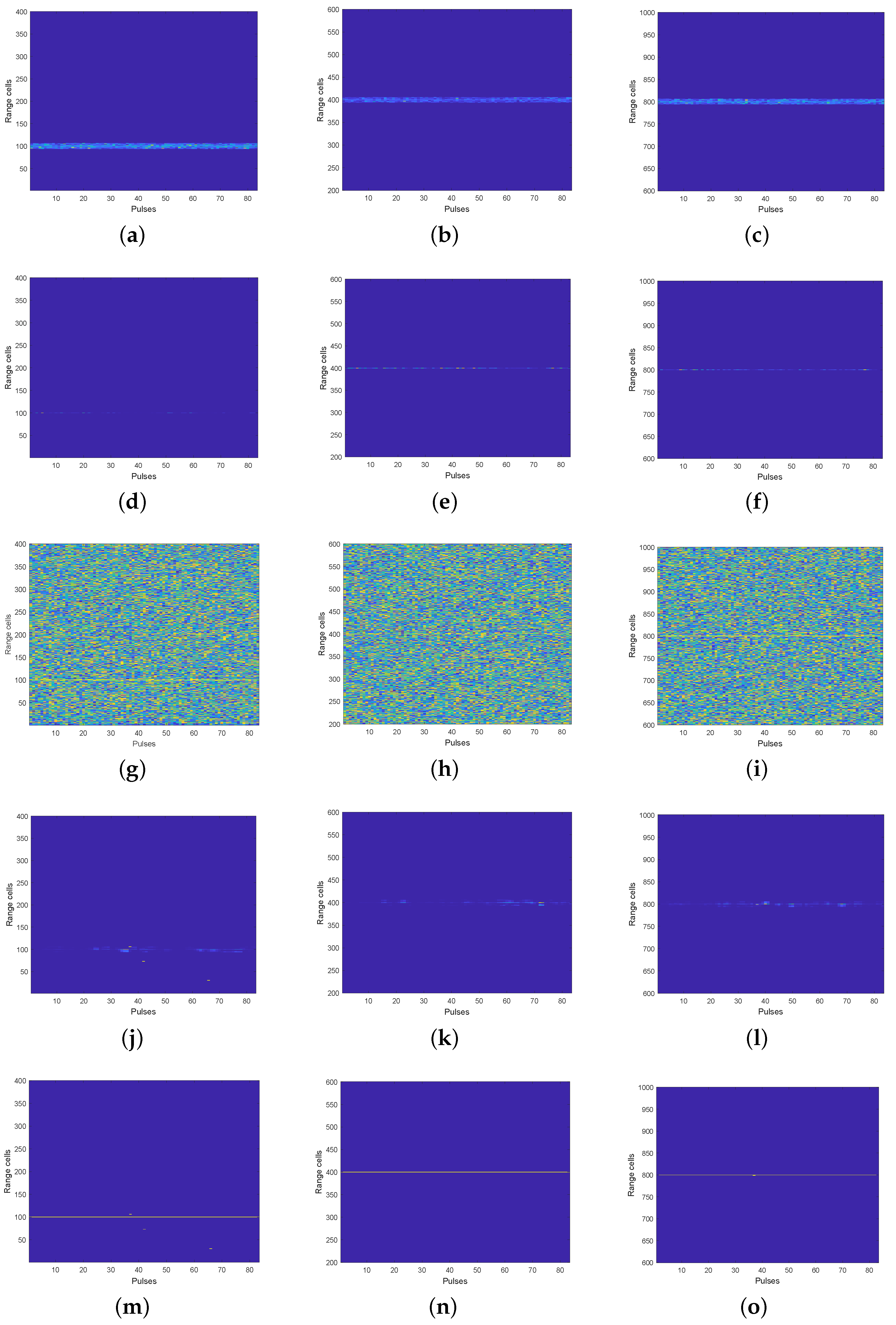
4.2. Experiments Based on Measured Data
4.2.1. Real Data of the Sea-Detecting Data-Sharing Program
4.2.2. Real Data of the Mountaintop Program
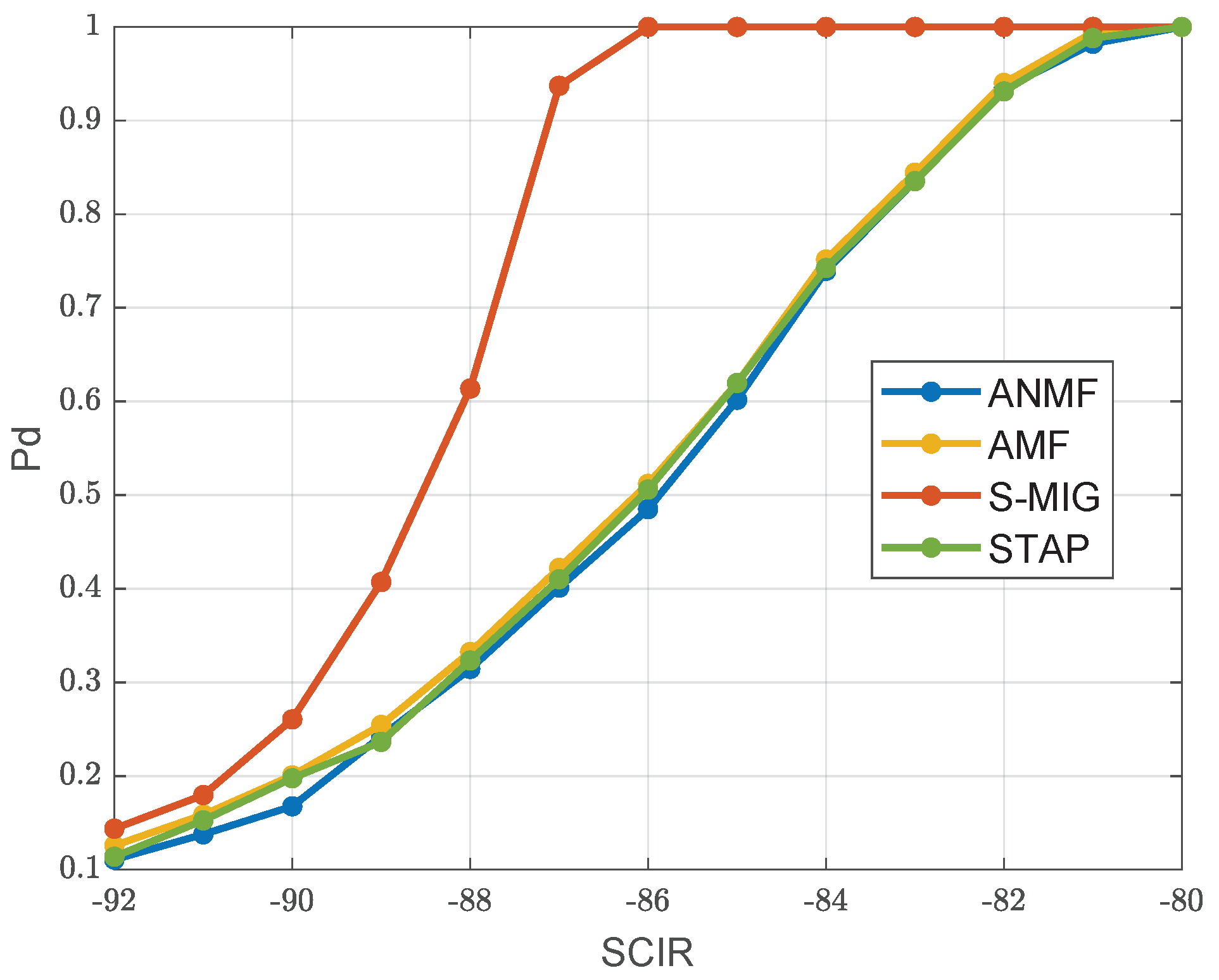
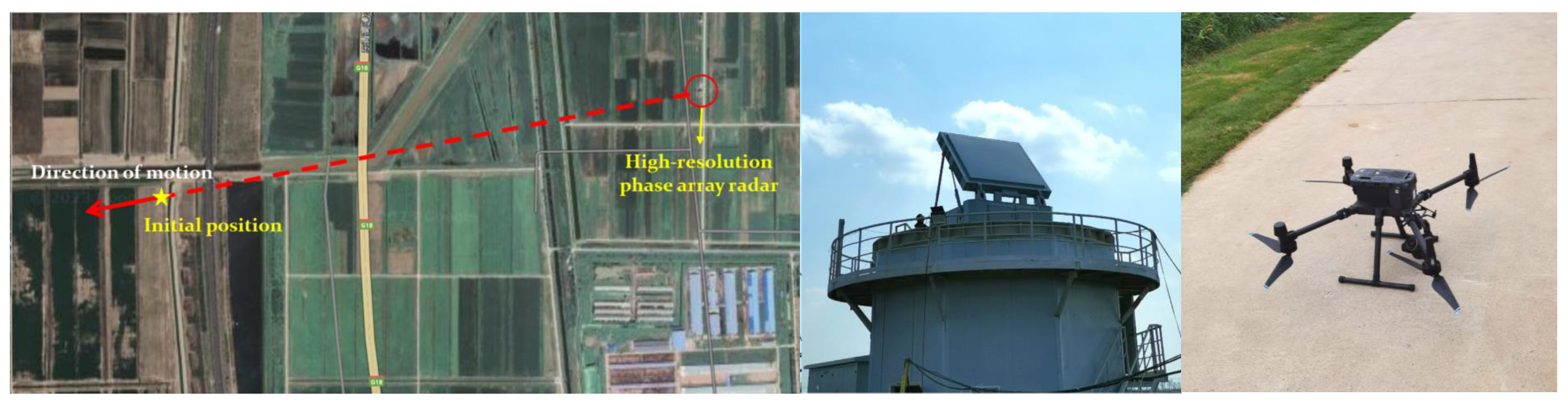
4.2.3. Real Data of the PHA Radar Database
5. Conclusions
Author Contributions
Funding
Data Availability Statement
Conflicts of Interest
Appendix A. Proof of Theorem
- In case I, according to Formula (30), we havewhere is the number of interference clutter patches. Therefore, we havewhere Equation (a) is established on both the property of the matrix inner product that and the equation that because is orthogonal to .
- In case II, as analyzed in Section 3.3.2, the hetero-clutter shows entirely different characteristics than the homo-clutter. We denote thatthenSimilar to (A5), in case II, we have
References
- Guerci, J.R. Space-Time Adaptive Processing for Radar, 2nd ed.; Artech House: Fitchburg, MA, USA, 2015; pp. 1–9. [Google Scholar]
- Reed, I.S.; Mallett, J.D.; Brennan, L.E. Rapid Convergence Rate in Adaptive Arrays. IEEE Trans. Aerosp. Electron. Syst. 1974, 10, 853–863. [Google Scholar] [CrossRef]
- Melvin, W.L. A STAP Overview. IEEE Aerosp. Electron. Syst. Mag. 2004, 19, 19–35. [Google Scholar] [CrossRef]
- Liu, W.; Xie, W.; Wang, Y. Diagonally Loaded Space-time Adaptive Detection. In Proceedings of the IEEE International Conference on Radar, Chengdu, China, 24–27 October 2011. [Google Scholar]
- Liu, W.; Xie, W.; Wang, Y. AMF and ACE Detectors Based on Diagonal Loading. Syst. Eng. Electron. 2013, 35, 463–468. [Google Scholar]
- Liu, W.; Liu, J.; Cao, C. Multichannel Adaptive Signal Detection: Basic Theory and Literature Review. Sci. China Inf. Sci. 2022, 65, 121301. [Google Scholar] [CrossRef]
- Wang, Y.; Liu, W.; Xie, W. Research Progress of Space-Time Adaptive Detection for Airborne Radar. J. Radars 2014, 3, 201–207. [Google Scholar] [CrossRef]
- Kelly, E.J. An Adaptive Detection Algorithm. IEEE Trans. Aerosp. Electron. Syst. 1986, 22, 112–127. [Google Scholar] [CrossRef]
- Chen, W.; Reed, I.S. A New CFAR Detection Test for Radar. Digit. Signal Process. 1991, 1, 198–214. [Google Scholar] [CrossRef]
- Robey, F.C.; Fuhrmann, D.R.; Kelly, E.J. A CFAR Adaptive Matched Filter Detector. IEEE Trans. Aerosp. Electron. Syst. 1992, 28, 208–216. [Google Scholar] [CrossRef]
- De Maio, A. Rao Test for Adaptive Detection in Gaussian Interference with Unknown Covariance Matrix. IEEE Trans. Signal Process. 2007, 55, 3577–3584. [Google Scholar] [CrossRef]
- De Maio, A. A New Derivation of The Adaptive Matched Filter. IEEE Signal Process. Lett. 2004, 11, 792–793. [Google Scholar] [CrossRef]
- Liu, W.; Xie, W.; Liu, J. Adaptive double subspace signal detection in Gaussian background—part. I: Homogeneous environments. IEEE Trans. Signal Process. 2014, 62, 2345–2357. [Google Scholar] [CrossRef]
- Liu, W.; Xie, W.; Gao, Y. Multichannel signal detection in interference and noise when signal mismatch happens. Signal Process. 2020, 166, 107268. [Google Scholar] [CrossRef]
- Liu, W.; Xie, W.; Liu, J. Adaptive double subspace signal detection in Gaussian background—part. II: Partially homogeneous environments. IEEE Trans. Signal Process. 2014, 62, 2358–2369. [Google Scholar] [CrossRef]
- Liu, W.; Gao, F.; Luo, Y. GLRT-based generalized direction detector in partially homogeneous environment. Sci. China Inf. Sci. 2019, 62, 209303. [Google Scholar] [CrossRef]
- Liu, W.; Wang, Y.; Liu, J. Adaptive detection without training data in colocated MIMO radar. IEEE Trans. Aerosp. Electron. Syst. 2015, 51, 2469–2479. [Google Scholar] [CrossRef]
- Liu, W.; Liu, J.; Huang, L. Rao tests for distributed target detection in interference and noise. Signal Process. 2015, 117, 333–342. [Google Scholar] [CrossRef]
- Introduction to Airborne Radar[M]. The Institution of Engineering and Technology; Geroge, W.S. (Ed.) SciTech Publishing: Raleigh, NC, USA, 2010. [Google Scholar]
- He, C.; Zhang, R.; Huang, B. Moving-Target Detection for FDA-MIMO Radar in Partially Homogeneous Environments. Electronics 2024, 13, 851. [Google Scholar] [CrossRef]
- Chen, X.; Cheng, Y.; Wu, H. Heterogeneous Clutter Suppression via Affine Transformation on Riemannian Manifold of HPD Matrices. IEEE Trans. Geosci. Remote Sens. 2022, 60, 5109816. [Google Scholar] [CrossRef]
- Yang, Y.; Yang, B. Overview of Radar Detection Methods for Low Altitude Targets in Marine Environments. J. Syst. Eng. Electron. 2024, 35, 1–13. [Google Scholar] [CrossRef]
- Kononov, A.A.; Ka, M.-H. Rapid Adaptive Matched Filter for Detecting Radar Targets with Unknown Velocity. IEEE Access 2024, 12, 25411–25428. [Google Scholar] [CrossRef]
- Conte, E.; De Maio, A. Mitigation Techniques for Non-Gaussian Sea Clutter. IEEE J. Ocean. Eng. 2003, 29, 284–302. [Google Scholar] [CrossRef]
- Gini, F.; Greco, M. Covariance matrix estimation for CFAR detection in correlated heavy tailed clutter. Signal Process. 2002, 82, 1847–1859. [Google Scholar] [CrossRef]
- Conte, E.; De Maio, A.; Ricci, G. Recursive estimation of the covariance matrix of a compound-Gaussian process and its application to adaptive CFAR detection. IEEE Trans. Signal Process. 2002, 50, 1908–1915. [Google Scholar] [CrossRef]
- Pailloux, G.; Forster, P.; Ovarlez, J.P. On Persymmetric Covariance Matrices in Adaptive Detection. In Proceedings of the IEEE International Conference on Acoustics, Speech and Signal Processing, Las Vegas, NV, USA, 31 March–4 April 2008. [Google Scholar]
- Pascal, F.; Chitour, Y.; Ovarlez, J.P. Covariance structure maximum likelihood estimates in compound-Gaussian noise: Existence and algorithm analysis. IEEE Trans. Signal Process. 2008, 56, 34–48. [Google Scholar] [CrossRef]
- Barbaresco, F. Innovative tools for radar signal processing based on Cartan’s geometry of SPD matrices & information geometry. In Proceedings of the IEEE Radar Conference, Rome, Italy, 26–30 May 2008. [Google Scholar]
- Arnaudon, M.; Yang, L.; Barbaresco, F. Stochastic algorithms for computing p-means of probability measures, geometry of radar Toeplitz covariance matrices and applications to HR Doppler processing. In Proceedings of the International Radar Symposium, Leipzig, Germany, 6–9 September 2011. [Google Scholar]
- Balaji, B.; Barbaresco, B. Application of Riemannian mean of covariance matrices to space-time adaptive processing. In Proceedings of the 9th European Radar Conference, Amsterdam, The Netherlands, 31 October–2 November 2012. [Google Scholar]
- Chen, X.; Cheng, Y.; Wang, H. Geometric Estimation on Manifolds Based Training Data Selection. In Proceedings of the 4th IEEE International Conference on Electronic Information and Communication Technology, Xi’an, China, 18–20 August 2021. [Google Scholar]
- Chen, X.; Cheng, Y.; Wu, H. Heterogeneous Clutter Suppression for Airborne Radar STAP Based on Matrix Manifolds. Remote Sens. 2021, 13, 3195. [Google Scholar] [CrossRef]
- Wu, H.; Cheng, Y.; Chen, X. Power Spectrum Information Geometry-Based Radar Target Detection in Heterogeneous Clutter. IEEE Trans. Geosci. Remote Sens. 2024, 62, 1–16. [Google Scholar] [CrossRef]
- Xie, Z.; Cheng, Y.; Wu, H. Ship Detection in SAR Images via Kullback-Leibler Divergence-Based Matrix Information Geometry Detector. J. Phys. Conf. Ser. 2023, 69, 4326. [Google Scholar] [CrossRef]
- Wu, H.; Cheng, Y.; Chen, X. Geodesic Normal Coordinate-Based Manifold Filtering for Target Detection. IEEE Trans. Geosci. Remote Sens. 2022, 60, 1–15. [Google Scholar] [CrossRef]
- Yang, Z.; Cheng, Y.; Wu, H. Enhanced Matrix CFAR Detection with Dimensionality Reduction of Riemannian Manifold. IEEE Signal Process. Lett. 2020, 27, 2084–2088. [Google Scholar] [CrossRef]
- Ye, L.; Yang, Q.; Chen, Q. Multidimensional Joint Domain Localized Matrix Constant False Alarm Rate Detector Based on Information Geometry Method with Applications to High Frequency Surface Wave Radar. IEEE Access 2019, 7, 28080–28088. [Google Scholar] [CrossRef]
- Ye, L.; Yang, Q.; Deng, W. Matrix Constant False Alarm Rate(MCFAR) Detector Based on Information Geometry. In Proceedings of the 2016 IEEE Information Technology, Networking, Electronic and Automation Control Conference, Chongqing, China, 20–22 May 2016. [Google Scholar]
- Yang, J.; Chen, Y.; Dirk, T.M. Signal Detection for Ultra-Massive MIMO: An Information Geometry Approach. IEEE Trans. Signal Process. 2024, 72, 824–838. [Google Scholar] [CrossRef]
- Wu, H.; Cheng, Y.; Chen, X. Adaptive Matrix Information Geometry Detector with Local Metric Tensor. IEEE Trans. Signal Process. 2020, 70, 3758–3773. [Google Scholar] [CrossRef]
- Yang, Z.; Cheng, Y.; Wu, H. Manifold Projection-Based Subband Matrix Information Geometry Detection for Radar Targets in Sea Clutter. IEEE Trans. Geosci. Remote Sens. 2023, 61, 1–15. [Google Scholar] [CrossRef]
- Wu, H.; Cheng, Y.; Chen, X. Information Geometry-Based Track-Before-Detect Algorithm for Slow-Moving Fluctuating Target Detection. IEEE Trans. Signal Process. 2023, 71, 1833–1848. [Google Scholar] [CrossRef]
- Chen, X.; Wu, H.; Cheng, Y. Joint Design of Transmit Sequence and Receive Filter Based on Riemannian Manifold of Gaussian Mixture Distribution for MIMO Radar. IEEE Trans. Geosci. Remote Sens. 2023, 61, 1–13. [Google Scholar] [CrossRef]
- Lapuyade-Lahorgue, J.; Barbaresco, F. Radar Detection Using Siegel Distance between Autoregressive Processes, Application to HF and X-band Radar. In Proceedings of the 2008 IEEE Radar Conference, Rome, Italy, 26–30 May 2008; pp. 1–6. [Google Scholar]
- Cheng, Y.; Hua, X.; Wang, H. The Geometry of Signal Detection with Applications to Radar Signal Processing. Entropy 2016, 18, 381. [Google Scholar] [CrossRef]
- Hua, X.; Peng, L.; Liu, W. LDA-MIG Detectors for Maritime Targets in Nonhomogeneous Sea Clutter. IEEE Trans. Geosci. Remote Sens. 2023, 61, 5101815. [Google Scholar] [CrossRef]
- Arnaudon, M.; Barbaresco, F.; Yang, L. Riemannian Medians and Means with Applications to Radar Signal Processing. IEEE J. Sel. Top. Signal Process. 2013, 7, 595–604. [Google Scholar] [CrossRef]
- Hua, X.; Yusuke, O.; Peng, L. Target Detection within Nonhomogeneous Clutter Via Total Bregman Divergence-Based Matrix Information Geometry Detectors. IEEE Trans. Signal Process. 2021, 69, 4326. [Google Scholar] [CrossRef]
- Hua, X.; Cheng, Y.; Wang, H. Matrix CFAR detectors based on symmetrized Kullback-Leibler and total Kullback-Leibler divergences. Digit. Signal Process. 2017, 69, 106–116. [Google Scholar] [CrossRef]
- Zhou, Z.; Hua, X.; Guan, C. Target Detection Based on Matrix Information Geometry for Continuous Active Sonar. J. Shaanxi Norm. Univ. 2019, 47, 23–29. [Google Scholar]
- Shi, Y.; Li, J. Target Detecting Algorithm Based on Subband Matrix for Slow Target in Sea Clutter. J. Electron. Inf. Technol. 2021, 43, 2703–2710. [Google Scholar]
- Zhao, W.; Jin, M.; Liu, W. Matrix CFAR Detector Based on Matrix Spectral Norm. Acta Electron. Sin. 2019, 47, 1951–1956. [Google Scholar]
- Ward, J. Space-Time Adaptive Processing for Airborne Radar; Lincoln Lab: Lexington, MA, USA, 1994; pp. 20–51. [Google Scholar]
- Conte, E.; Lops, M.; Ricci, G. Asymptotically Optimum Radar Detection in Compound-Gaussian Clutter. IEEE Trans. Aerosp. Electron. Syst. 1995, 31, 617–625. [Google Scholar] [CrossRef]
- Adve, R.; Hale, T.; Wicks, M. Knowledge Based Adaptive Processing for Ground Moving Target Indication. Digit. Signal Process. 2007, 17, 495–541. [Google Scholar] [CrossRef]
- Guan, J.; Liu, N.; Wang, G. Sea-detecting radar experiment and target feature data acquisition for dual polarization multistate scattering dataset of marine targets. J. Radars 2023, 12, 456–469. [Google Scholar]
- Liu, N.; Dong, Y.; Wang, G. Sea-detecting X-band radar and data acquisition program. J. Radars 2019, 8, 656–667. [Google Scholar]
- Hu, C.; Yan, Y.J.; Wang, R. High-resolution, Multi-frequency and Full-polarization Radar Database of Small and Group Targets in Clutter Environment. Sci. China Inf. Sci. 2023, 66, 227301. [Google Scholar] [CrossRef]
- Titi, G.W.; Marshall, D.F. The ARPA/NAVY Mountaintop Program: Adaptive Signal Processing for Airborne Early Warning Radar. In Proceedings of the 1996 IEEE International Conference on Acoustics, Speech and Signal Processing, Atlanta, GA, USA, 9 May 1996. [Google Scholar]
- Titi, G.W. An Overview of the ARPA/NAVY Mountaintop Program. In Proceedings of the 1994 IEEE Long Island Section Adaptive Antenna Systems Symposium, Melville, NY, USA, 19 November 1992. [Google Scholar]
- Carlson, B.D.; Goodman, L.M.; Asutin, J. An Ultralow-Sidelobe Adaptive Array Antenna. Linc. Lab. J. 1990, 3, 291–310. [Google Scholar]
- The Development of E-2D Radar from the Radar Monitoring Technology Experimental Radar RSTER to the E-2C RMP Project. Available online: http://www.360doc.com/content/18/0126/21/13664199_725368484.shtml (accessed on 1 May 2024).


| Detector | Step I | Step II | Step III | Summary |
|---|---|---|---|---|
| AMF | ||||
| ANMF | ||||
| MIG | ||||
| S-MIG |
| Parameters | Clutter | Hetero-Clutter in Case I | Hetero-Clutter in Case II |
|---|---|---|---|
| N | 4 | 4 | 4 |
| P | 6 | 6 | 6 |
| n | - | 24 | 24 |
| 0.6 | 0.6 | 0.1 | |
| 20 dB | 20 dB | 5 dB | |
| 0.2 | 0.2 | 0.8 | |
| shape parameter v | 0.4 | 0.4 | 0.4 |
| scale parameter b | 0.6 | 0.6 | 0.6 |
| number of interference | 0 | 2 | 0 |
| - | (0.2, 0.2) | - | |
| - | (0.2, 0.9) | - | |
| (0.55, 0.55) | - | - |
| Parameter | Symbol | Value |
|---|---|---|
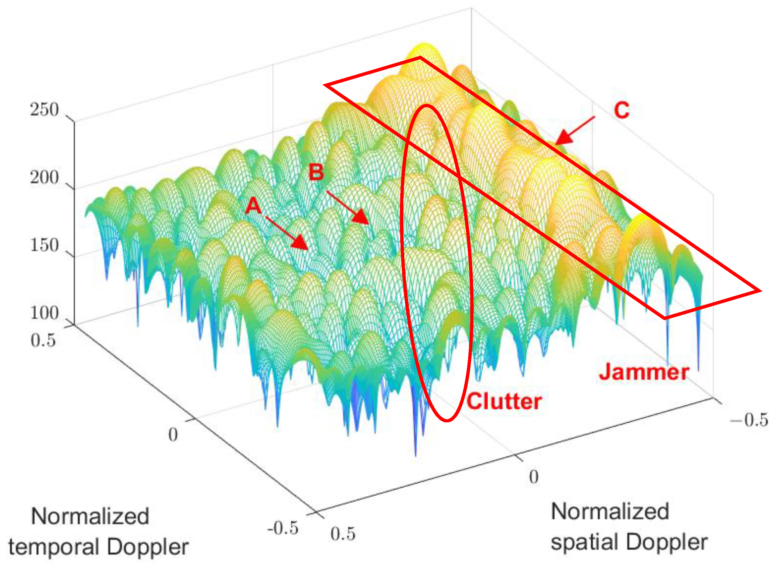
| Doppler for target A | (0.25, —0.16) | |
| Doppler for target B | (0.01, —0.16) | |
| Doppler for target C | (—0.41, —0.16) | |
| DoF | M | 224 |
| number of reference cells | K | 28 |
| number of guard cells | - | 1 |
| CPI sequence number | cpi | 1 |
| AMF | ANMF | STAP | S-MIG | |
|---|---|---|---|---|
| Target A | —81.06 dB | —81.05 dB | —81.08 dB | —85.63 dB |
| Target B | —78.69 dB | —79.03 dB | —78.62 dB | —81.76 dB |
| Target C | —79.65 dB | —79.66 dB | —79.63 dB | —84.88 dB |
| Method | SCNR | Method | SCNR |
|---|---|---|---|
| STAP without CFAR | 16.626 dB | AMF | 28.831 dB |
| CA-CFAR after STAP | 12.559 dB | ANMF | 7.751 dB |
| OS-CFAR after STAP | 12.255 dB | MIG | 17.977 dB |
| GO-CFAR after STAP | 12.888 dB | S-MIG | 32.060 dB |
Disclaimer/Publisher’s Note: The statements, opinions and data contained in all publications are solely those of the individual author(s) and contributor(s) and not of MDPI and/or the editor(s). MDPI and/or the editor(s) disclaim responsibility for any injury to people or property resulting from any ideas, methods, instructions or products referred to in the content. |
© 2024 by the authors. Licensee MDPI, Basel, Switzerland. This article is an open access article distributed under the terms and conditions of the Creative Commons Attribution (CC BY) license (https://creativecommons.org/licenses/by/4.0/).
Share and Cite
Zou, R.; Cheng, Y.; Wu, H.; Yang, Z.; Hua, X.; Wu, H. A Steering-Vector-Based Matrix Information Geometry Method for Space–Time Adaptive Detection in Heterogeneous Environments. Remote Sens. 2024, 16, 2208. https://doi.org/10.3390/rs16122208
Zou R, Cheng Y, Wu H, Yang Z, Hua X, Wu H. A Steering-Vector-Based Matrix Information Geometry Method for Space–Time Adaptive Detection in Heterogeneous Environments. Remote Sensing. 2024; 16(12):2208. https://doi.org/10.3390/rs16122208
Chicago/Turabian StyleZou, Runming, Yongqiang Cheng, Hao Wu, Zheng Yang, Xiaoqiang Hua, and Hanjie Wu. 2024. "A Steering-Vector-Based Matrix Information Geometry Method for Space–Time Adaptive Detection in Heterogeneous Environments" Remote Sensing 16, no. 12: 2208. https://doi.org/10.3390/rs16122208