Article

Non-Destructive Monitoring of Peanut Leaf Area Index by Combing UAV Spectral and Textural Characteristics

1
College of Geodesy and Geomatics, Shandong University of Science and Technology, Qingdao 266590, China
2
Institute of Crop Germplasm Resources, Shandong Academy of Agricultural Sciences, Jinan 250100, China
3
College of Natural Resources and Environment, Northwest A&F University, Xianyang 712100, China
*
Author to whom correspondence should be addressed.
Remote Sens. 2024, 16(12), 2182; https://doi.org/10.3390/rs16122182
Submission received: 9 May 2024 / Revised: 12 June 2024 / Accepted: 13 June 2024 / Published: 16 June 2024
(This article belongs to the Section Remote Sensing in Agriculture and Vegetation)

Abstract

:
The leaf area index (LAI) is a crucial metric for indicating crop development in the field, essential for both research and the practical implementation of precision agriculture. Unmanned aerial vehicles (UAVs) are widely used for monitoring crop growth due to their rapid, repetitive capture ability and cost-effectiveness. Therefore, we developed a non-destructive monitoring method for peanut LAI, combining UAV vegetation indices (VI) and texture features (TF). Field experiments were conducted to capture multispectral imagery of peanut crops. Based on these data, an optimal regression model was constructed to estimate LAI. The initial computation involves determining the potential spectral and textural characteristics. Subsequently, a comprehensive correlation study between these features and peanut LAI is conducted using Pearson’s product component correlation and recursive feature elimination. Six regression models, including univariate linear regression, support vector regression, ridge regression, decision tree regression, partial least squares regression, and random forest regression, are used to determine the optimal LAI estimation. The following results are observed: (1) Vegetation indices exhibit greater correlation with LAI than texture characteristics. (2) The choice of GLCM parameters for texture features impacts estimation accuracy. Generally, smaller moving window sizes and higher grayscale quantization levels yield more accurate peanut LAI estimations. (3) The SVR model using both VI and TF offers the utmost precision, significantly improving accuracy (R2 = 0.867, RMSE = 0.491). Combining VI and TF enhances LAI estimation by 0.055 (VI) and 0.541 (TF), reducing RMSE by 0.093 (VI) and 0.616 (TF). The findings highlight the significant improvement in peanut LAI estimation accuracy achieved by integrating spectral and textural characteristics with appropriate parameters. These insights offer valuable guidance for monitoring peanut growth.

1. Introduction

Peanuts are an important economic and oil crop in China. In 2022, the total peanut production in China was approximately 18,329,000 tons, accounting for more than half of the national oil crop production [1]. Their high and stable yields are crucial for ensuring national oil security and promoting sustainable agricultural development. The leaves of peanuts and their distribution play a fundamental role in photosynthesis [2] and evapotranspiration [3], exerting a crucial influence that significantly shapes the developmental status of peanut crops. LAI, which denotes the cumulative leaf region ratio against the ground region, stands as a paramount biophysical parameter crucial for assessing the growth of crop populations, diagnosing its nutrient status and predicting yields [4,5] since it can accurately characterize crop canopy structures as well as quantitatively analyze many physical and biological processes of crop ecosystems. Therefore, rapid and non-destructive monitoring of peanut LAI is of great significance for guiding precise agronomic management and yield estimations of peanuts.
Traditional destructive LAI measurements primarily depend on field sampling, which causes damage to the crop leaves during the acquisition process [6]. This approach is not only time-consuming and demanding, but also fails to meet the crucial demand for real-time monitoring. Although the non-destructive monitoring of LAI can be achieved using hand-held optical devices, e.g., SunScan plant canopy analyzer and Li-Cor LAI-2000, it usually requires the professional experience of operators, making it difficult to address the issue of real-time monitoring at the field scale [7]. With the advancement and application of remote sensing techniques, this method has been successfully used for large-scale crop growth monitoring in recent years. It can achieve rapid, large-scale, and non-destructive monitoring of crop biophysical and biochemical parameters [8], offering an effective alternative to traditional destructive or optical-based LAI measurements. Various payloads of remote sensing work on different platforms, e.g., ground, aerial, and space, according to their height above the ground to implement the specific monitoring tasks [9,10]. Among these platforms, unmanned aerial vehicles (UAVs), as an emerging aerial observation platform, have been increasingly popular in the field of crop growth monitoring [11] due to its practical advantages, such as its rapid, repetitive capture ability and low cost. More importantly, UAVs carrying high-resolution sensors produce centimeter-level or even higher imagery, providing rich information related to crop growth.
To date, numerous LAI estimation methods based on UAV-based remote sensing have been presented and are generally divided into two groups: physical models and empirical statistical models. The physical models are mainly divided into two types: physical radiative transfer models [12] and photogrammetry-based models [13,14]. The key insight behind the former is the mechanism of the reflection and absorption between the sunlight and the crop canopy. Due to the complex formula and many required parameters of physical radiative transfer models, they might be prone to the issue of pathological inversion [15]. The latter is commonly used for LAI inversion of forests and is not suitable for low and dwarf crops such as peanuts. Unlike the physical models, empirical statistical models explore the assumption that the crop’s characteristic parameters have significant correlations with its LAI [16], and the characteristics derived from remote sensing data are correlated with the plot-scale LAI values using several empirical statistical methods [17,18]. Since they are user-friendly and straightforward to implement, the empirical statistical methods are increasingly popular and used in this work.
In many instances, the empirical statistical approach used to estimate LAI involves constructing a regression model between LAI and the spectral reflectance of derived vegetation indices. This is because canopy reflectance offers the most immediate indication of vegetation characteristics. Many previous studies have calculated and evaluated numerous vegetation indices, applying the estimation of LAI and achieving good results. For example, Cao et al. [17] developed a wide dynamic range vegetation index (WDRVI) that added a weight coefficient to the normalized difference vegetation index (NDVI) for NIR and improved the accuracy of sugar beet growth monitoring. Ilniyaz et al. [19] compared the effects of vegetation indices derived from multispectral and red, green, and blue (RGB) data on the LAI estimation, revealing that multispectral data show excellent potential for LAI estimations in vineyards, with an accuracy of 0.889 (R2) and 0.434 (RMSE). These previous studies have made significant contributions to investigations of the relationship between LAI and vegetation indices. As a matter of fact, the spectral reflectance and its derived VIs are insensitive to the dynamic changes in crop canopy growth. As is well known, when the biomass of crops is high, the vegetation indices exhibit saturation, which might degrade the accuracy of the LAI estimation model when solely relying on these indices.
In contrast to the spectral reflectance that focuses on the crop’s internal optical responses, texture features reflect the external morphological characteristics of the crop, offering rich spatial structure information on the crop canopy [20]. Therefore, the capability of texture features in capturing the dynamic changes in crop canopy growth makes it suitable for improving the precision of LAI estimations. Despite the low precision observed when using texture features alone [21,22], the integration of both spectral and texture features has shown superior potential in previous studies related to LAI estimation [22,23,24,25,26] and has been demonstrated to alleviate the phenomenon of spectral saturation [26,27]. For instance, Wang et al. [24] linearly combined texture features to form the normalized difference texture index (NDTI), which is integrated with spectral features to effectively enhance the accuracy for retrieving mixed grass LAI. Also, Yuan et al. [26] combined spectral and texture features to estimate rice LAI. Among the four regression models used, the SVR model provides the best accuracy for the estimation, which suggests that the feature combination solution (R2 = 0.917, RMSE = 0.078) surpasses the performance of the spectral features alone (R2 = 0.839, RMSE = 0.017).
Although numerous methods have been developed and provide promising LAI estimation results for rice [20,26], potato [28,29], maize [30,31], and other crops by combining both VI and TF to date, it is still remarkably challenging due to the following aspects. First, despite the combination of both, VI and TF have been demonstrated to have important value for monitoring LAIs of multiple crops; as far as we are aware, fewer studies specifically address the effect of both vegetation indices and texture features on the peanut LAI estimation since differences in the canopy structures of different crops might lead to changes in texture characteristics as well as spectral absorption and reflection characteristics. Moreover, texture features exhibit significant sensitivity to both the window size and the grayscale quantity level in the GLCM parameters. Nevertheless, few studies comprehensively investigate the effects of GLCM-based texture features for peanut LAI estimation [32]. Second, previous studies have successfully combined both VI and TF to optimize the accuracy of LAI estimations. However, they often input a substantial number of features into the training model without scoring the importance of both VI and TF.
In response to the aforementioned challenges, we propose a non-destructive monitoring method for peanut LAI that integrates texture and spectral information derived from UAV multispectral imagery. Our main contributions in this work are as follows.
(1)
An exhaustive and meticulous correlation analysis between the spectral/textural characteristics and peanut LAI is carried out using a feature variable screening technique to determine the optimal feature combination in estimating the peanut LAI.
(2)
Several key parameters for calculating GLCM-derived statistical measures from the high-resolution UAV remote sensing data are investigated to evaluate the effect on the performance of the peanut LAI estimation model.
(3)
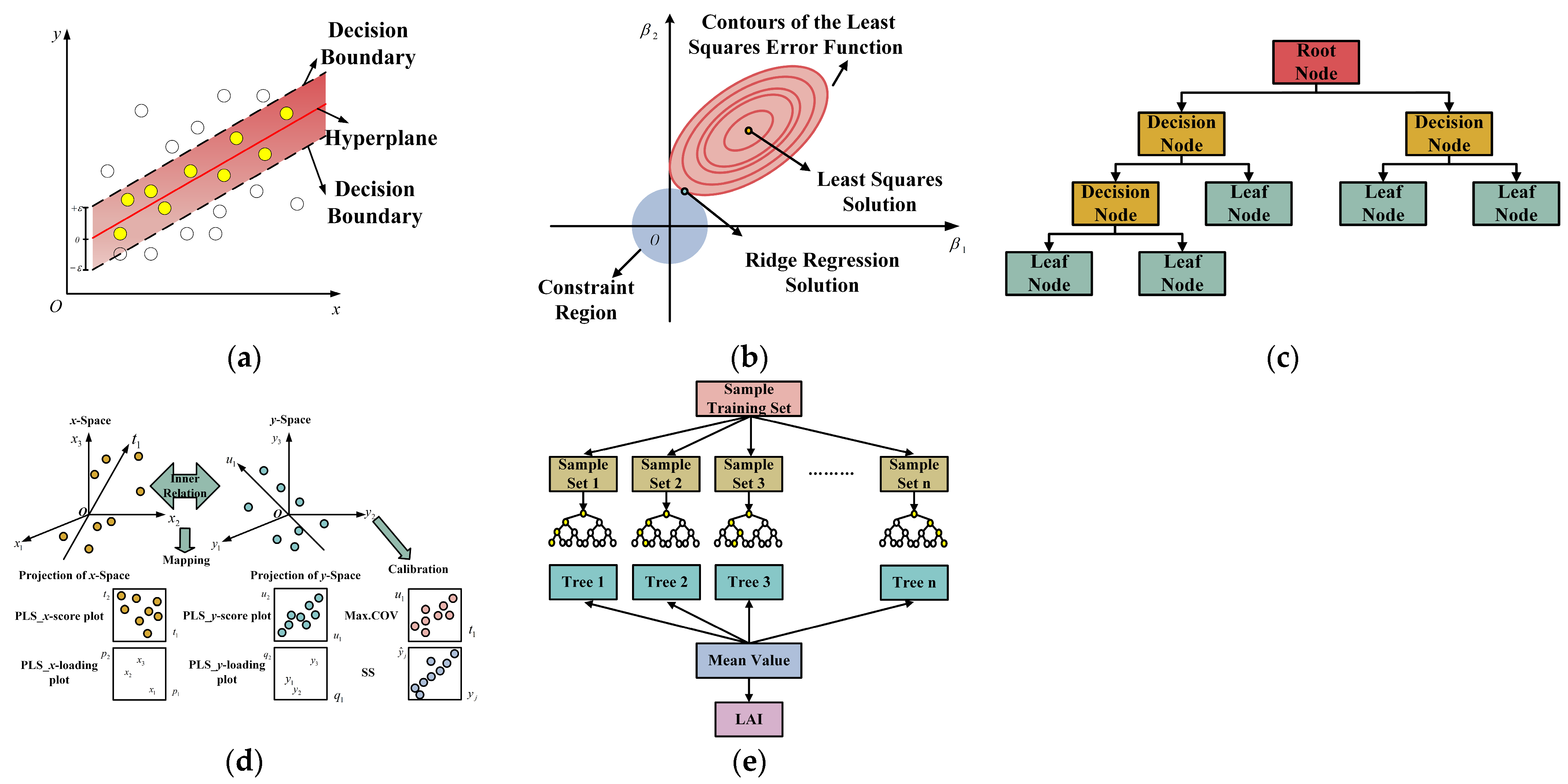
Different combinations of both spectral and textural characteristics are systematically compared and evaluated using six frequently used regression methods, including ULR, SVR, RR, DTR, PLSR, and RFR, to determine the optimal estimation of peanut LAI.
The rest of this paper is organized as follows. Section 2 present an introduction to the study site and data collection. Following this, the methodology, including feature extraction and selection as well as model construction and optimization, is described in Section 3. Section 4 showcases the experimental implementations and results of this work. Section 5 is dedicated to the discussion of our findings and a overview of our future research.

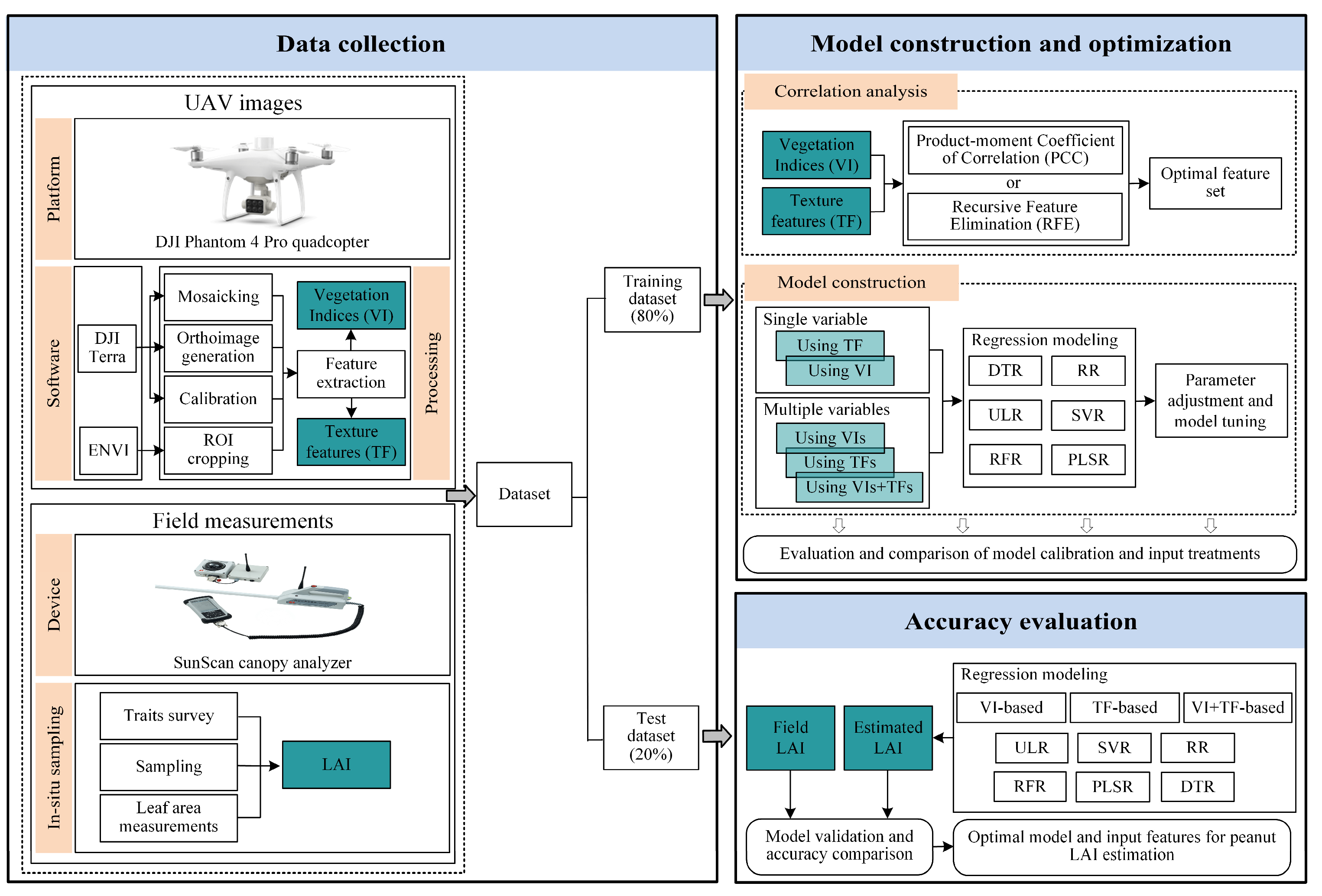
2. Material and Methods

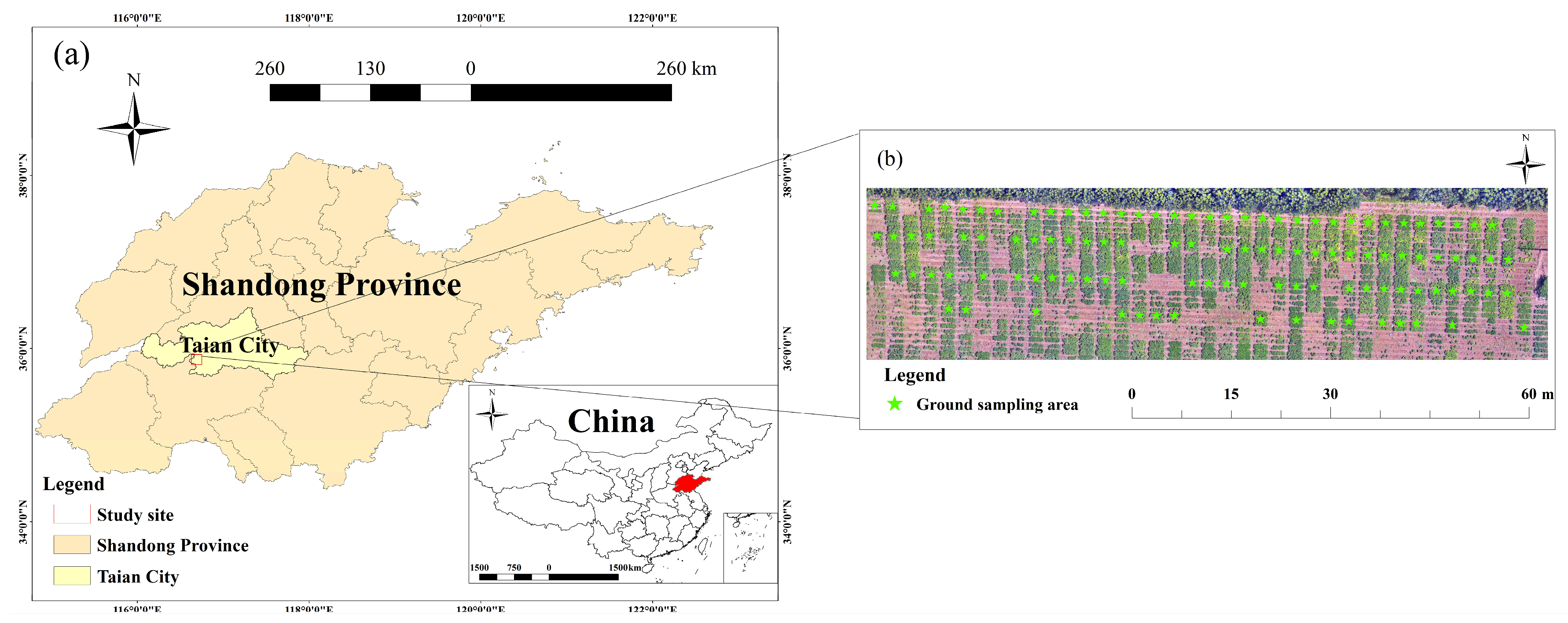
2.1. Description of Study Site

The study area is located in Ningyang county, Tai’an city, Shandong province, China (116°39′56″E, 35°50′15″N), as shown in Figure 1. It is a typical area with a semi-humid warm-temperate continental climate that is characterized by distinct four seasons with simultaneous rain and heat, and its annual average temperature is approximately 14 °C. The average altitude of this county is 85 m, with an annual average sunshine duration of 2759.1 h, an annual average precipitation of 901.4 mm, and an annual average frost-free period of 199 days. The research area adopts a coordinate system under UTM zone 49 N projection, using WGS84 as a geodetic datum.

2.2. Field Data Collection

In our experiments, 1000 peanut plots were planted with the same fertilizer (15 kg KH2PO4/ha, 15 kg urea/ha) and irrigation treatments. Watering is carried out in a timely fashion according to the growth requirements of peanuts. Ridge planting was adopted for the plot, with each plot area measuring 1 m2 and a row spacing of 0.5 m. In this study, we used the SunScan canopy analyzer to measure LAI and a drone to obtain multispectral images. In situ data observations started on 31 May 2023, and concluded on 23 August 2023. The operation was carried out on sunny days from 8:00 to 10:00 to avoid direct sunlight and obtain more uniform lighting conditions. For each plot, the three-point sampling method was used to obtain the truth value. Specifically, three representative sampling points were selected to represent the growth status, and their corresponding LAI values were measured with the SunScan plant canopy analyzer. As a result, the average of representative sampling points for each plot was considered as its fielded LAI.

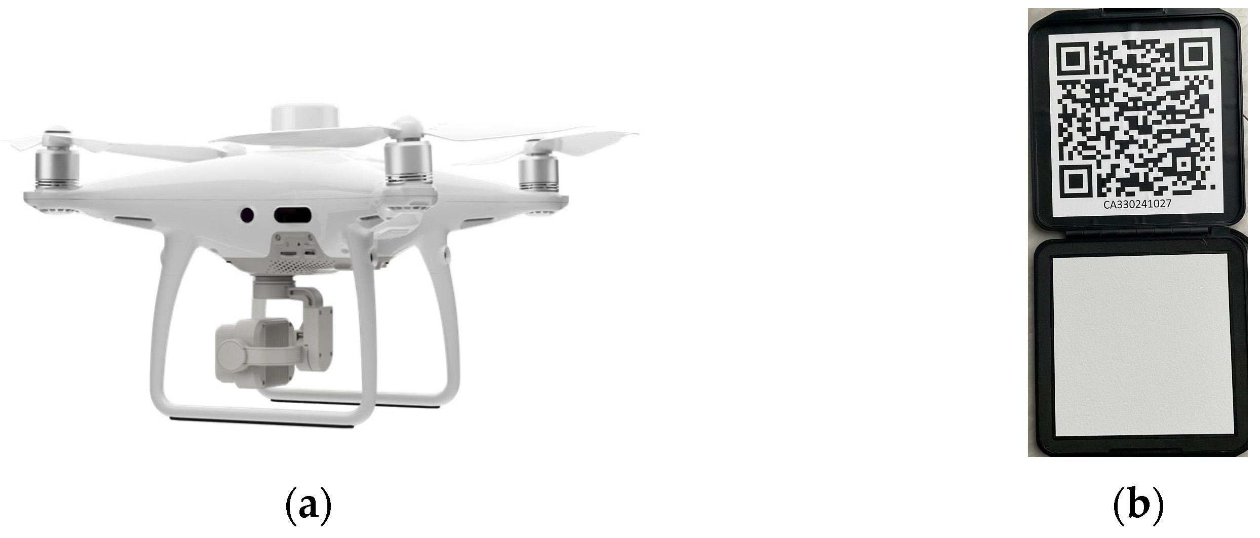
2.3. UAV Imagery Acquisition

DJI Phantom 4 multispectral quadcopter (Shenzhen DJI Sciences and Technologies Ltd., Shenzhen, China) was used as a remote sensing platform for high-resolution imagery collection with a takeoff weight of 1.38 kg and a range of 30 min, as shown in Figure 2a. It is equipped with a complementary metal oxide semiconductor (CMOS) sensor and an integrated multispectral imaging system, which consists of one visible light band and five multispectral bands (i.e., red (R), green (G), blue (B), NIR-red (NIR) and red-edge (RE) bands), as listed in Table 1. Due to the large field area, drone data collection is divided into two flight missions. During all flight missions, in order to avoid shadow interference caused by direct sunlight, each flight mission is conducted between 10 a.m. and 2 p.m. Before the drone took off, a standard whiteboard was placed horizontally on the ground, and it was photographed from a height of 1.2 m to facilitate radiometric calibration, as shown in Figure 2b. Radiometric calibration was performed three times for each spectral band prior to every flight. To improve positioning accuracy, we utilized the DJI GS Pro platform for flight route planning and display. During this process, we set the longitudinal overlap to 80% and the lateral overlap to 60% with a flight altitude of 20 m above ground level and a spatial resolution of 0.86 cm per pixel. Afterwards, DJI terra software 3.7.0 was applied to align the aerial images with the position and orientation system (POS) and mosaic them to generate the digital orthophoto map (DOM) of the study area. Following this, ENVI 5.3.1 software was adopted to perform clipping operations for the minimum bounding rectangle of the regions of interest, generating the average reflectance of each plot (a total of 111 plots) for subsequent spectral and texture feature calculations.

2.4. Methods

2.4.1. Calculation of Spectral Characteristics

The vegetation index refers to a parameter obtained by combining two or more reflectance bands linearly or nonlinearly that describe their characteristics in relation to chlorophyll content and LAI. According to the relevant literature, we selected 15 common vegetation indices with good results in LAI monitoring for field crops in previous studies. The selected Vis are briefly described, and their specific calculation formulas are listed in Table 2. More specifically, a region of interest (ROI) of a fixed size that fits the corresponding plot as largely as possible using the ROI tool in ENVI 5.3.1 software is first cropped to compute the fixed-size plot’s spectral characteristics. Following this, the plot-scale canopy reflectance is considered as the average of all of the pixels’ values within it. Consequently, the selected plot-scale VI is computed from its canopy reflectance. Figure 3 visualizes fifteen vegetation indices according to the values of the associated vegetation features.

2.4.2. Calculation of Texture Characteristics

Texture features are the specific arranged patterns that exist within a certain range of an image, reflecting the visual characteristics of homogeneity and the arrangement properties of the surface patterns. GLCM, as a statistical method that considers the spatial pattern arrangements, is achieved by analyzing the grayscale level variants of an image, which are related to the spatial statistics. Therefore, in this work, we used GLCM to extract statistical measures to represent the texture features of the image. These GLCM-derived statistical measures offer an explicit or implicit representation of the repeating pattern of local intensity variations. Table 3 provides a brief description of texture features. In our implementation, ENVI 5.3.1 software is also explored to produce the GLCM on five spectral bands and derive several statistical parameters, including mean (MEA), variance (VAR), contrast (CON), correlation (COR), dissimilarity (DIS), entropy (ENT), second moment (SEM), and homogeneity (HOM), from the calculated GLCM. Figure 4 visualizes eight GLCM-derived texture features according to the values of the associated texture feature.

2.4.3. Screening of Spectral and Texture Characteristics

As previously mentioned, we empirically summarize and compute all potential spectral/textural characteristics derived from UAV multispectral images, including 15 vegetation indices and 40 texture features, since they have been widely and successfully used to estimate and map plant canopy LAI from multispectral remote sensing data [24,31]. Among these characteristics, many of them might be highly correlated with other characteristics or have no correlation to the in situ LAI, which would result in poor performance in peanut LAI estimations [45]. To effectively alleviate irrelevancy and redundancy without losing significant information, it is very necessary to find a subset of useful spectral/textural characteristics from the total of 15 vegetation indices and 40 textural characteristics. In this work, we used two screening techniques: Pearson’s product-moment coefficient of correlation (PCC) [46] and recursive feature elimination (RFE) [28,47].
(1) Pearson’s product-moment coefficient of correlation (PCC) is the most commonly used statistical criterion to measure the correlation between two continuous variables, which is often denoted as r [ 1 ,   1 ] using the following formula. For a detailed explanation of r , please refer to Kurtz’s research [48]. After producing the correlation coefficient r , the two-tailed significance test is further carried out to offer the statistical evidence for a linear relationship, which is often denoted by P [49]. Generally speaking, a higher value of r denotes a stronger linear relationship, while a lower P -value signifies a more statistically significant association.
r = i = 1 n ( x i x ~ ) ( y i y ~ ) / ( n 1 ) i = 1 n ( x i x - ) 2 / ( n 1 ) i = 1 n ( y i y - ) 2 / ( n 1 )
Here, x i and y i are the values of two variables x and y, respectively (i.e., spectral/textural characteristics and LAI in this work); x - and y - are the average value of two variables x and y, respectively; and n is the number of data.
(2) Recursive feature elimination (RFE) operates as a wrapper-type method for feature selection by ranking features based on their own importance. Technically, it finds a subset of useful features by recursively fitting the given machine learning algorithm, scoring the features, and then discarding the weakest features until the specified number of features remains.

2.4.4. Construction of Regression Models

Once the spectral and textural characteristics of the LAI are computed, the spectral characteristics, textural characteristics, or a combination of both serve as the input of machine learning-based regression approaches to determine their relationships with in situ LAI values, where the spectral characteristics are denoted as “VI”, the textural characteristics are denoted as “TF”, and a combination of both is denoted as “VI + TF”. In our implementation, six frequently used regression models, including ULR, SVR, RR, DTR, PLSR, and RFR, are chosen to investigate whether “VI + TF” is conductive to peanut LAI estimations. Figure 5 provides a theoretical diagram of the five regression models.
(1) The univariate linear regression (ULR) model is a simple and common linear regression model that focuses on the approximate linear relationship between the remote sensing variable (e.g., spectral, texture) and the peanut LAI. Generally, it is fitted as a univariate linear equation using the least-square approach, as listed in Equation (2):
y = b x + a
where y is the peanut LAI, x is the single remote sensing variable, and b and a are the slope and the intercept of the fitted line of the univariate linear regression model, respectively.
(2) Support vector regression (SVR) is a widely used machine learning-based estimation method due to its versatility, robustness, and effectiveness. Moreover, it can effectively handle high-dimensional data and nonlinear problems, with a superior generalization ability [50]. The key insight behind it is to project the input samples onto a high-dimensional space, where a hyperplane is established. Following this, the loss function derived from the distances between the training samples and the hyperplane is minimized by only considering the input samples outside the hyperplane, as shown in Figure 5a. As a consequence, the hyperplane is the fitted regression model.
(3) Ridge regression (RR) is an extended linear regression model for alleviating multicollinearity problems, where a regularization term is added to the loss function. Figure 5b visualizes the theoretical diagram of the RR model. This regularization term is equivalent to the sum of the squared weight coefficients multiplied by the regularization strength. By doing this, the values of the weight coefficients are reduced but not completely to zero, effectively controlling the complexity of the model, avoiding overfitting and enhancing the model’s generalization ability.
(4) The decision tree regression (DTR) model divides the dataset by recursively selecting the best features and thresholds, making the samples in each subset as similar as possible. This iteration continues until a specified stopping condition is met, exemplified by reaching a predetermined tree depth or the number of samples in the node dropping below a certain threshold. Decision tree regression adopts a tree structure, where each node represents the decision condition of a feature variable, and its leaf node contains a predicted continuous value that is usually the average of all samples within it, as shown in Figure 5c.
(5) Partial least squares regression (PLSR) is a statistical technique that integrates the advantages of multiple linear regression and principal component analysis (PCA). Figure 5d provides a theoretical diagram of a PLSR model. It usually requires a good linear relationship between the remote sensing variable (e.g., spectral and texture) and the peanut LAI. With regards to the estimation situation of LAI, in which there are many remote sensing variables with complex interweaving correlations, traditional linear regression cannot accurately achieve the goal of LAI estimation, while PLSR is simple and stable and provides high prediction accuracy.
(6) Random forest regression (RFR) consists of multiple decision trees, each trained on diverse subsets extracted from the same training set. General speaking, RFR uses a bootstrap technique, where each bootstrap is continuously trained to minimize the sum of squared residuals until a complete tree is formed, as shown in Figure 5e. Noted that each tree is built based on a random sampling of data, and the trees are then combined into a “forest” for the regression task. Compared to decision tree regression, RFR uses random sampling during the branching process, ensuring that the global optimal decision is returned. Previous work has demonstrated that RFR effectively handles high-dimensional data and a large number of data, without being affected by overfitting [25], and shows a certain degree of robustness for dealing with nonlinear relationships and outliers.

2.4.5. Assessment of Regression Models

The procedure used for statistical analysis after data collection and model construction is summarized in Figure 6. For all the in situ data, we randomly split them into training and test sets to establish and evaluate the regression model, separately. The ratio of the training and test split is 80% and 20%, respectively. In our implementation, we compare the performance of six regression models for peanut LAI estimations using VI, TF, and VI + TF, separately, and we adopt the determination coefficient (R2) and root mean square error (RMSE) to quantitatively evaluate the consistency between estimated and measured LAI values, as listed in Equations (3) and (4). For the former, a value closer to 1 indicates superior model estimation performance. As for the latter, it indicates the degree of deviation between estimated and measured values, with a smaller value corresponding to better model estimation performance. All of statistical analysis are carried out using the Python programming language (https://www.python.org, accessed on 30 April 2024).
R 2 = 1 i = 1 N ( y ^ i y i ) 2 i = 1 N ( y i y - ) 2
R M S E = i = 1 N ( y ^ i y i ) 2 N
Here, y i denotes the measured LAI value, y ^ i denotes the estimated LAI value, y - denotes the average value, and N denotes the total number of samples.

3. Result and Analysis

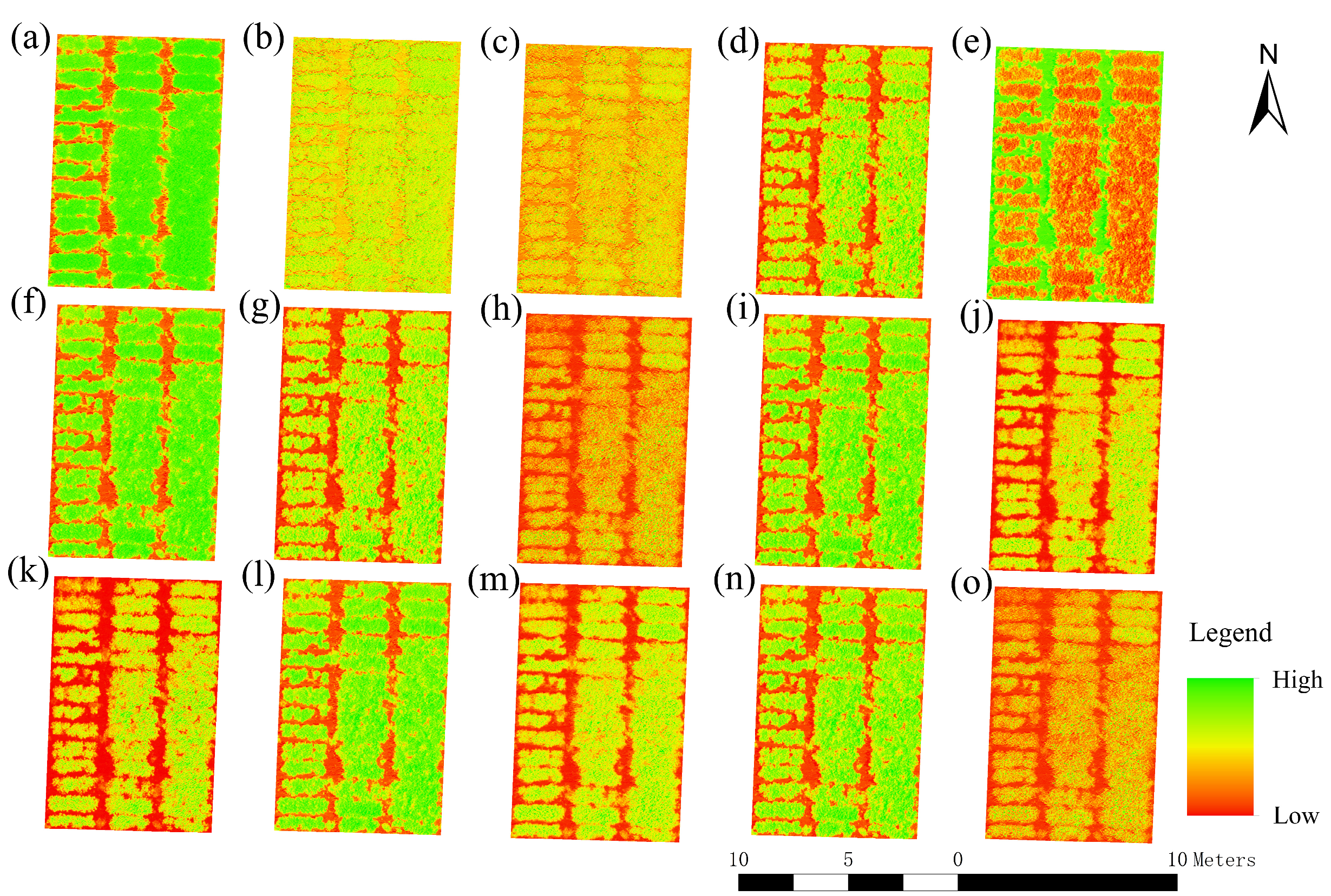
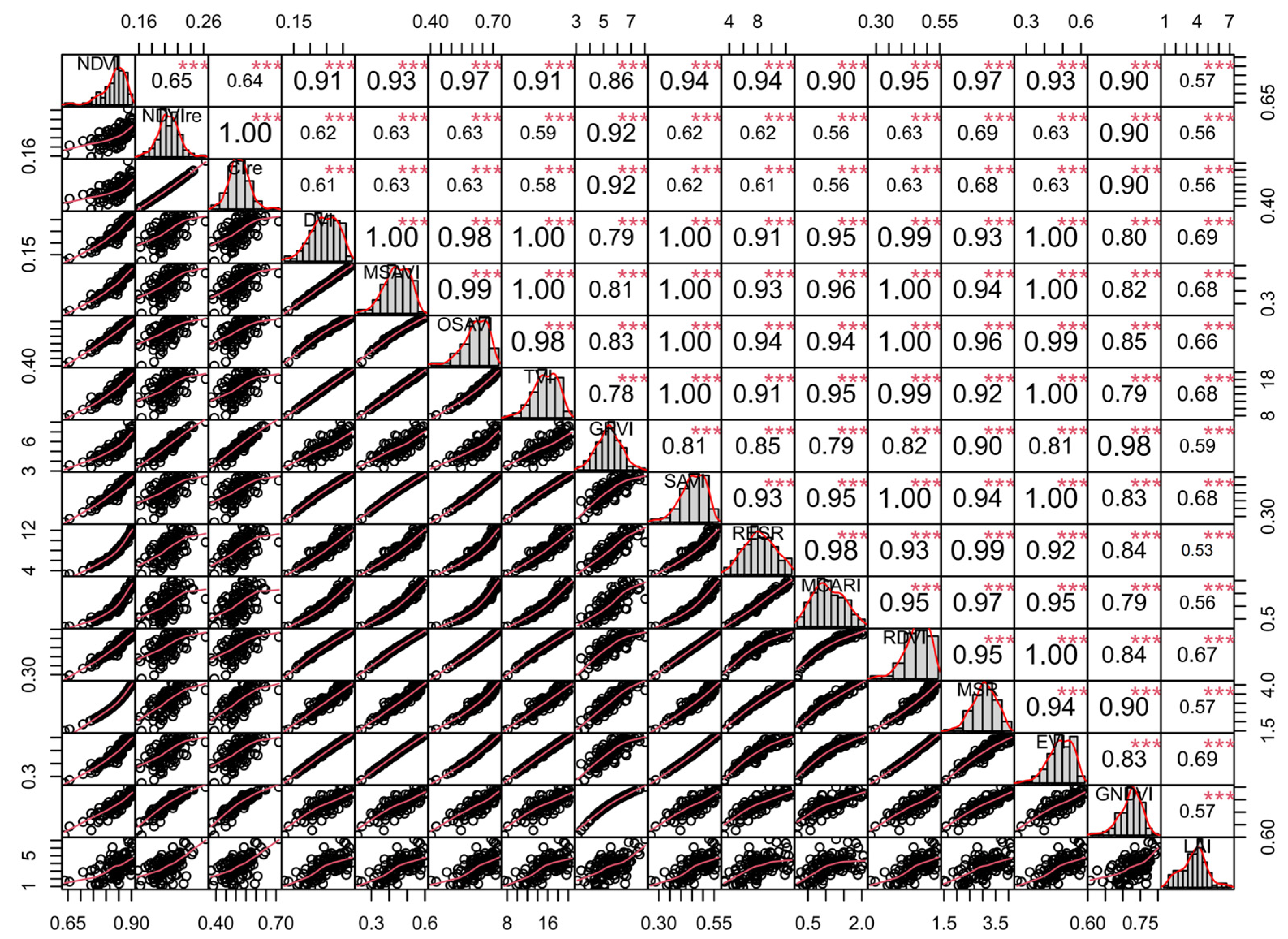
3.1. Correlation Analysis between LAI and Vegetation Indices

A correlation analysis was conducted between the calculated 15 vegetation indices and the measured LAI, and the Pearson’s correlation coefficients are shown in Figure 7. The last row and last column in the figure describe the correlation between LAI and various vegetation indices, while the rest describes the correlation between various vegetation indices. The findings demonstrate that the correlation coefficients between all the calculated vegetation indices and LAI are greater than 0.53, and the correlation coefficients between each vegetation index are greater than 0.56, indicating a high degree of correlation among the variables. Among these vegetation indices, DVI, EVI, and LAI have the strongest correlation, with the highest correlation coefficient of 0.69, while RESR offers the weakest correlation, with lowest correlation coefficient of 0.53. Consequently, all vegetation indices are retained and ranked as DVI (0.69), EVI (0.69), TVI (0.68), MSAVI (0.68), SAVI (0.68), RDVI (0.67), OSAVI (0.66), GRVI (0.59), MSR (0.57), NDVI (0.57), GNDVI (0.57), MCARI (0.56), CIre (0.56), NDVIre (0.56), and RESR (0.53) according to their own correlation coefficients.

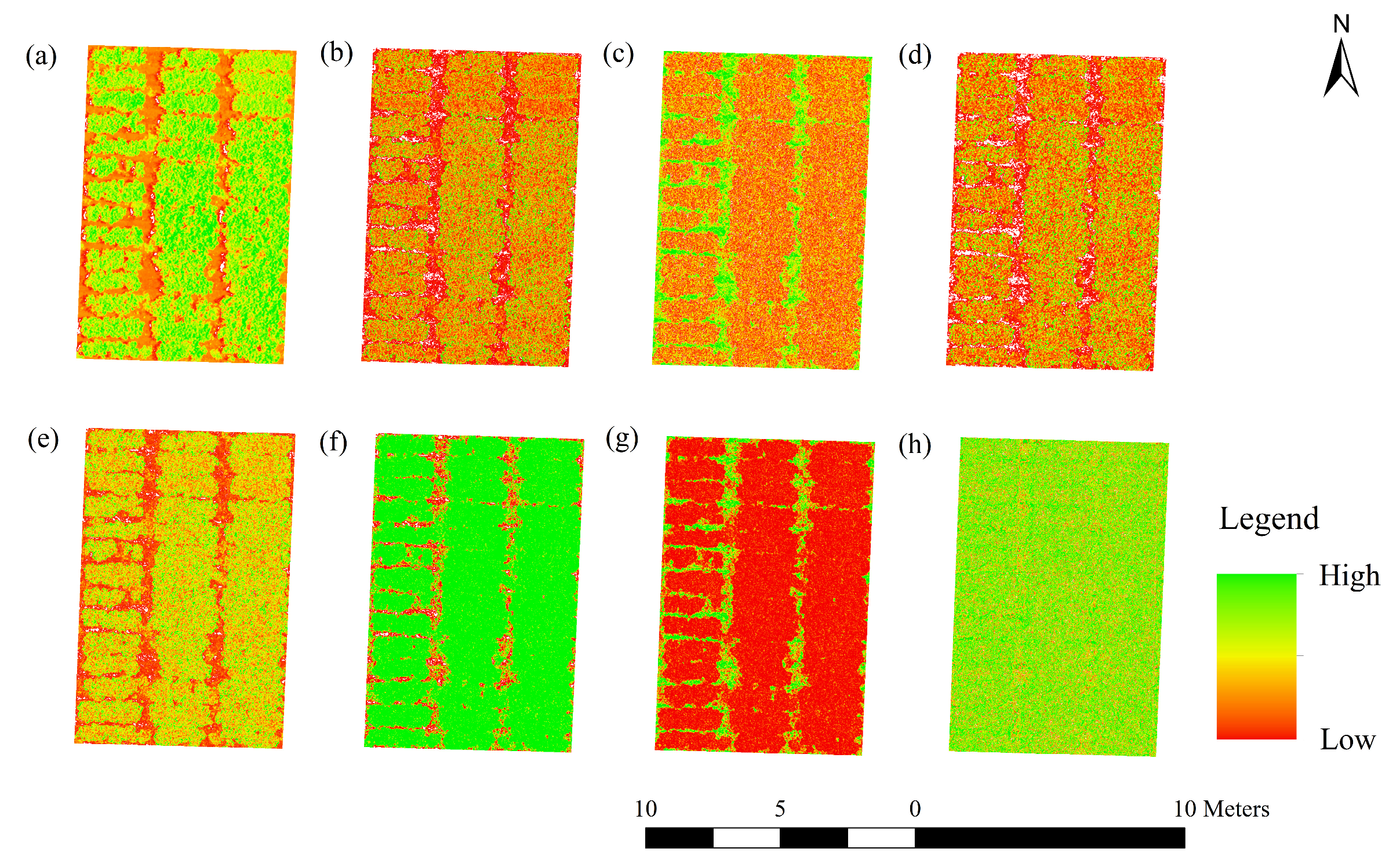
3.2. Correlation Analysis between LAI and Texture Features

Correlation analysis was also performed between the extracted 40 texture features and the measured LAI, and the Pearson correlation coefficients are presented in Table 4. The results indicate that more than half of the texture features were weakly correlated with LAI, with only a small portion showing a strong correlation with LAI. For example, among them, the correlation between MEA and LAI was relatively high, with correlation coefficients of 0.610 for the blue band, 0.570 for the red-edge band, and 0.610 for the NIR-red band. Previous studies [22,51] have also demonstrated that the textural characteristics derived from R, RE, and NIR bands are beneficial to the LAI estimation. Based on the results of previous studies and our findings from the correlation analysis between variables (as shown in Figure 8), a total of 20 texture features were selected, including blue-COR, blue-MEA, green-COR, green-MEA, red-SEC, red-ENT, red-DIS, red-HOM, red-COR, RE-MEA, RE-COR, RE-SEC, RE-VAR, RE-DIS, NIR-MEA, NIR-COR, NIR-SEC, NIR-DIS, NIR-HOM, and red-MEA.

3.3. RFE Processing for Feature Selection

In order to effectively alleviate irrelevancy and redundancy without losing useful spectral and texture information, we implement the feature scoring using the RFE-SVR method to screen for a useful feature set. The importance of each feature derived from Section 3.1 and Section 3.2 is shown in Figure 8. During the process of constructing the RFE-SVR model, we eliminate several weak features until convergence. The results indicate that the importance of features derived from the NIR and RE bands rank higher than the other bands, suggesting that the NIR and RE bands are more sensitive to peanut LAI. As a result, 9 features are retained for the establishment of the optimal peanut LAI estimation model, including 3 vegetation indices (GRVI, MCARI, and TVI) and 6 texture features (blue-MEA, NIR-SEC, NIR-HOM, NIR-DIS, RE-DIS, and RE-VAR).

3.4. Estimation of Peanut LAI with Texture Features

The high-resolution images of peanuts from the UAV platform have rich geometric structure and spatial information [52], which can provide rich spatial and structural information on the crops’ canopy for LAI estimation. In this work, we investigate the role of texture features in LAI estimation by constructing multiple regression models based on texture features alone. Moreover, the key parameters, including the size of the moving window and the grayscale quantization level, for calculating GLCM features are also systematically analyzed. Figure 9 demonstrates the accuracy of models based on different parameters for calculating GLCM features. The results indicate that it is evident that the estimation results are suboptimal. When the parameter settings are set with a moving window size of 3 × 3 and a grayscale quantization level of 64, the estimation accuracy is highest (SVR: R2 = 0.326, RR: R2 = 0.309, DTR: R2 = 0.349, PLSR: R2 = 0.357, and RFR: R2 = 0.283). Based on the above results, the performance of LAI estimations using texture features alone is very poor, which is also consistent with observations from previous studies [22].

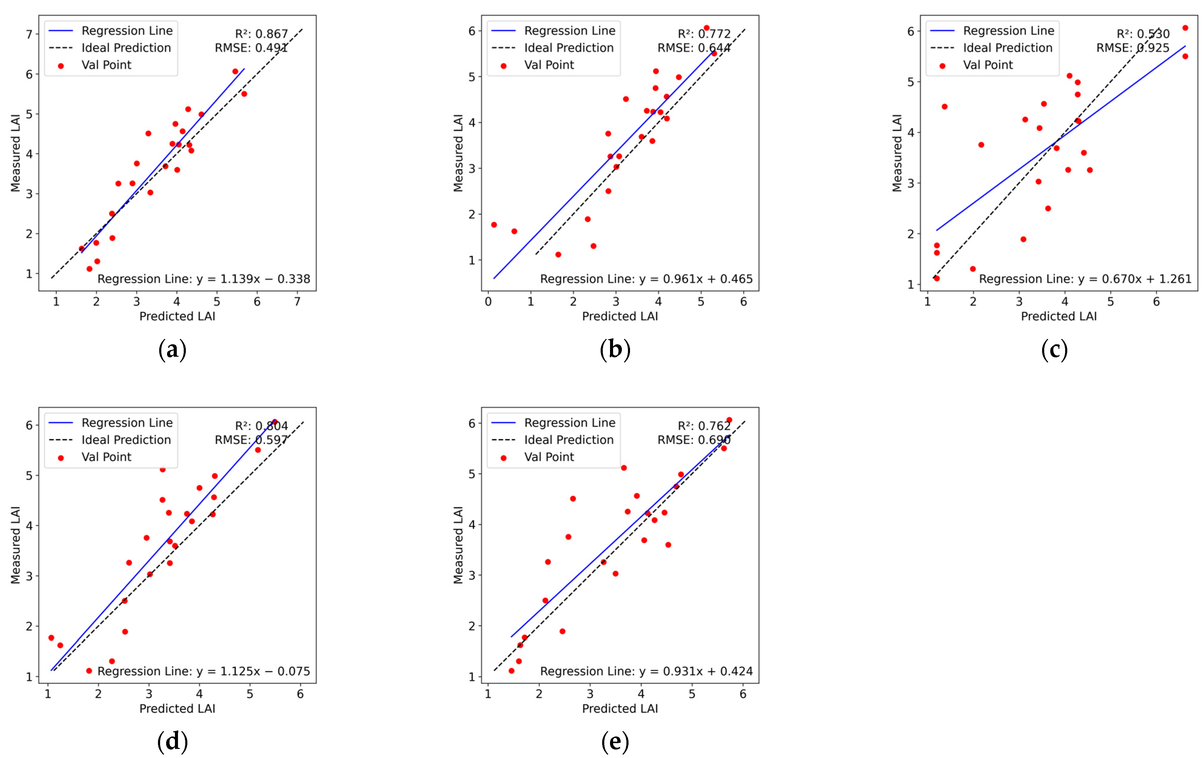
3.5. LAI Estimation Based on Different Characteristics

To delve deeper into the capabilities of spectral and texture features, this work also assesses the accuracy of different combinations of these characteristics using univariate linear regression models and multivariate regression models to find the optimal model for estimating peanut LAI. First, Table 5 summarizes the ULR’s accuracy for LAI estimation. Among the univariate linear models based on VI alone, the TVI-based model performs the best, with accuracy values of 0.545 for R2 and 0.770 for RMSE, while among the counterparts based on TF alone, the S E M 2 -based model offers highest R2 value of 0.309 and an RMSE of 0.950. By comparing the results of the univariate linear regression models, it was observed that the models based on vegetation indices exhibited higher accuracy than those of texture features. Nevertheless, the accuracy of these models was generally low, making it difficult to meet the requirements for high-quality estimation of peanut LAI.
With regards to the multivariate regression models using VI, TF, and VI + TF, we also observed that there are significant differences in estimation accuracy among different regression models, as listed in Table 6. The accuracy of estimation using VI + TF usually outperforms estimations using VI or TF alone.
Among the multivariate regression models based on VI alone, the SVR model performs the best, with accuracy values of 0.812 for R2 and 0.584 for RMSE, while among the counterparts based on TF alone, the PLSR model offers highest R2 value of 0.357 and the highest RMSE of 1.082, which suggests that the multivariate regression models using VI alone generally have higher accuracy than those using TF alone. By constructing a regression model that combines VI and TF, the accuracy of the model was significantly improved. Among five constructed regression models, the SVR model still offers the highest accuracy, with accuracy values of 0.867 for R2 and 0.491 for RMSE. Moreover, the combination of VI and TF is superior to VI alone (R2 = 0.812, RMSE = 0.584) and TF alone (R2 = 0.326, RMSE = 1.107). Similarly, RR, DTR, PLSR, and RFR models exhibit similar performance, indicating that combining vegetation index and texture features can effectively improve the performance of the LAI estimation.

3.6. Comparison of Various Multivariate Regression Methods

In addition to the selection of feature sets, the regression algorithms themselves are another key factor that affect the accuracy of LAI estimations. For the estimation of peanut LAI, this work used five multiple regression methods for comparative analysis to search for the most suitable method, including SVR, RR, DTR, PLSR, and RFR, for peanut LAI estimation. Figure 10 demonstrates estimation results of different models for peanut LAI using a combination of VI and TF. From the results, we found that SVR had the best performance, with R2 = 0.867 and RMSE = 0.491, followed by the PLSR model, with R2 = 0.804 and RMSE = 0.597, which bears resemblance to the research results [53] due to the fact that SVR can effectively handle the issues of nonlinearity and spectral noise in the dataset and exhibit a strong generalization ability on small sample data. Also, the performance of DTR is significantly the worst model (R2 = 0.530, RMSE = 0.856). This may be because the learning of decision trees is based on greedy algorithms, which attempt to achieve overall optimality by optimizing local optima; however, the global optimal decision tree is not always guaranteed, causing the problem of overfitting.

4. Discussion

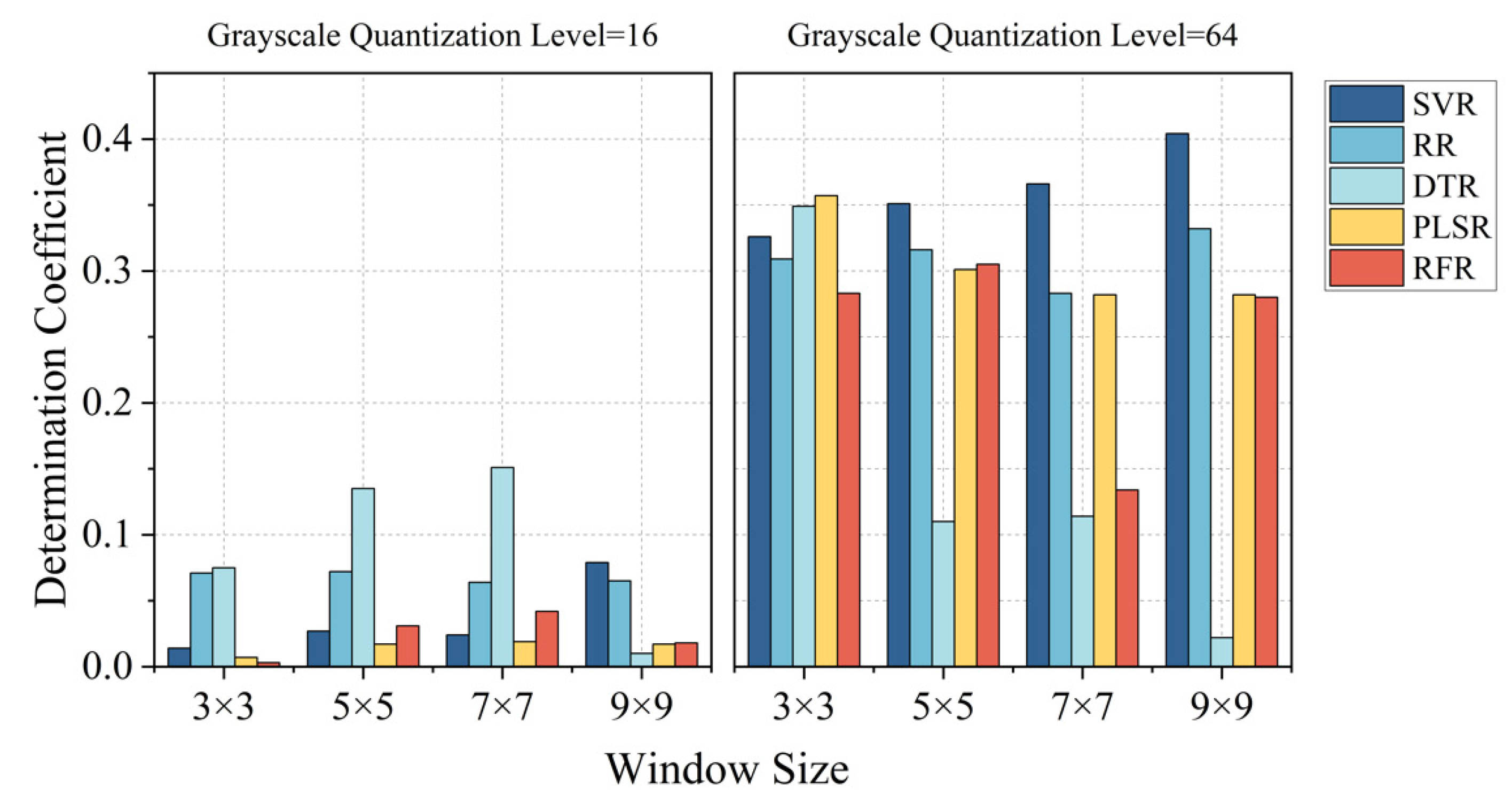
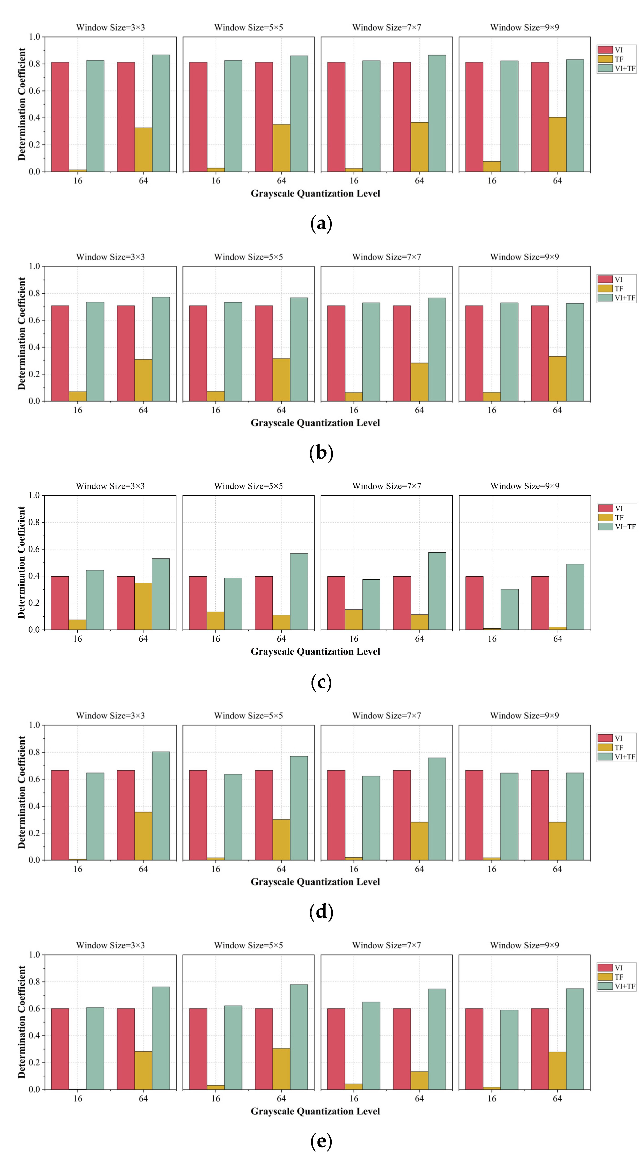
4.1. Effects of GLCM Parameters on the Performance of LAI Estimation

The size of the moving window and the grayscale quantization level are important parameters for extracting CGLM-derived TF. In theory, the smaller the size of the moving window and the higher the quantization level are, the better the information can reflect finer and richer texture features [32]. In our implementation, we set the size of moving windows to 3 × 3, 5 × 5, 7 × 7, and 9 × 9 as well as the grayscale quantization level as 16 and 64. Table 7 and Figure 11 indicate coefficients of determination (R2) for the LAI estimation of peanut from VI, TF, and VI + TF under different GLCM parameter settings.
Based on our experimental results, it could be found that the estimation accuracy of peanut LAI decreases as the moving window size increases. When the size of the moving window is 3 × 3, the LAI estimation has the highest accuracy, which conforms to Zhou’s research [54]. They found that when using texture features to study the LAI of black locality, the R2 values of the 3 × 3 and 5 × 5 windows are higher than those of the 7 × 7 or 9 × 9 windows since the small moving windows are more sensitive to the differences in the proportion of vegetation canopy, which is conducive to improving the accuracy of the estimation. Although small moving windows can capture texture changes on a small scale, sparsity and instability might be caused if it is too small [55], which is also be confirmed in the previous work [56].
What’s more, we also find that a grayscale quantization level of 64 generally has a higher accuracy than that of 16. However, previous studies [57] concluded that increasing the quantization level of GLCM texture features might reduce the accuracy of the results and that a quantization level higher than 64 not only fails to improve accuracy but also significantly increases computational complexity. At present, few studies have delved into the effect of the grayscale quantization level on the results when using a grayscale co-occurrence matrix to extract texture features, which to some extent hinders its value.
To sum up, when the moving window size is 3 × 3 and the grayscale quantization level is 64, the model has the best estimation accuracy (R2 = 0.867, RMSE = 0.491). This discovery suggests that the accuracy of LAI estimation can be markedly enhanced through the utilization of suitable texture parameters.

4.2. Advantages and Limitations of the Developed LAI Estimation Model

The vegetation indices are widely employed for estimating LAI and other crop growth parameters in the field of precision agriculture, and many previous studies [19,58] have achieved promising estimation results. In this work, we screened 3 vegetation indices, namely MCARI, GRVI, and TVI, using both PCC and RFE methods and then constructed multiple regression models using these three variables, obtaining accuracy values of 0.812 for R2 and 0.584 for RMSE, which further confirm the potential of VI in estimating peanut LAI. Nevertheless, as the peanut’s fraction vegetation coverage increases, the vegetation indices fail to reflect the interior structural information of the crop canopy; therefore, the estimation based on the vegetation indices alone could degrade [59].
The spatial information of high-resolution remote sensing data, such as texture, is related to the spatial structure of crops and can more effectively reflect the shadow and the interior structural information of the crop canopy. It has great potential in estimating forest biomass, LAI, and biodiversity [60]. With regards to texture features based on GLCM, they are extracted from all bands of the multispectral imagery and explored to assess their effect on peanut LAI estimation. Using correlation analysis, it was found that most texture features have a weak correlation with LAI. For the univariate linear regression model based on texture features alone, the highest accuracy values are 0.309 for R2 and 0.950 for RMSE. Among the five constructed regression models, the SVR model still offers the highest accuracy, with accuracy values of 0.867 for R2 and 0.491 for RMSE. As a consequence, the LAI estimation model based on texture features alone shows a poor performance, which is similar to the viewpoint of the previous work [22].
As a matter of fact, the vegetation indices and texture features offer information on the peanut’s canopy structures from their own perspectives, which is beneficial to the LAI estimation. In our implementation, it could be concluded that the accuracy of the model constructed by combining VI and TF has been significantly improved, with the highest accuracy values of 0.867 for R2 and 0.491 for RMSE. Furthermore, it remarkably outperforms VI alone, with differences of 0.055 in R2 and 0.093 in RMSE, or TF alone, with differences of 0.541 in R2 and 0.616 in RMSE. Thus, we conclude that the combination of VI and TF is helpful in the LAI estimation of peanuts, and this notion is also consistent with some previous work [22,31].
Drones have the characteristics of high spatial resolution and high temporal resolution and can be used to obtain a large range of high-resolution spectral images in a short period of time, effectively compensating for the shortcomings of satellite remote sensing in small- and medium-sized high-precision estimation research and representing a new tool in the field of precision agriculture [61]. To date, there have been numerous studies on drone remote sensing for estimating LAI of crops such as corn [51,62], winter wheat [56,63], and rice [20,26]. In our work, we further confirm the practical potentials of drone remote sensing for estimating peanut LAI.
In this work, we established one optimal estimation model for peanut LAI by screening various vegetation indices and texture features. In our implementation, we only used the data from one field with the same fertilizer application, cropping pattern, etc. to establish and validate our estimation model. Because of the differences noted for other fields (e.g., different fertilizer, irrigation treatments, or cropping patterns) or data from multiple years, fluctuations in the performance of the estimation model might occur [64]. As a consequence, the generalization of the LAI estimation model will be validated in our future research. In addition to spectral and texture information, some horizonal and vertical structures of a crop’s canopy, such as the color characteristics of crops, fraction vegetation coverage (FVC), plant height (PH), etc., also have the potential to impact the estimation of LAI since they could reflect the crop’s canopy structures from their own perspectives. Lots of previous studies [22,23,28] have used a combination of horizonal and vertical structure characteristics of the crop’s canopy for LAI estimation.

5. Conclusions

In the pursuit of a more accurate estimation of peanut LAI, this work compares the performance of spectral and texture information from UAV multispectral data for LAI estimation. Moreover, based on the construction of a useful feature set, six frequently used regression methods are explored to systematically compare and evaluate the model’s accuracy based on different combinations of input. Consequently, an optimal estimation method for peanut LAI was determined. The following conclusions are drawn:
(1)
The integration of two feature selection methods, PCC and RFE, was used to identify 9 useful spectral and textural characteristics that contribute significantly to peanut LAI, including 3 vegetation indices (GRVI, MCARI, and TVI) and 6 texture features (blue-MEA, NIR-SEC, NIR-HOM, NIR-DIS, RE-DIS, and RE-VAR).
(2)
The parameter settings when extracting texture features have an impact on the estimation results. For high-resolution images obtained using drones, the smaller the size of the moving window and the higher the grayscale quantization level are, the higher the accuracy of the estimation of peanut LAI.
(3)
The estimation model that combines VI and TF effectively enhances the accuracy of LAI prediction, achieving an R2 of 0.867 and an RMSE of 0.491.
This work provides a practical method for monitoring crop growth using drone imagery. To further improve the model’s accuracy and reliability, color, FVC, PH, etc., will be introduced into our LAI estimation model in future work.

Author Contributions

D.Q., J.Y. and Z.L. conceived and designed the research. B.B., G.L. and J.W. conducted field experiments and data acquisition. J.L. (Jincheng Liu) and J.L. (Jiayin Liu) developed the algorithms and performed the data analysis. D.Q. and J.Y. wrote the first draft and revised it based on suggestions from the other authors. All authors have read and agreed to the published version of the manuscript.

Funding

This research was jointly funded by the Shandong Provincial Key Research and Development Program (grant numbers 2022LZGC021 and 2021LZGC026) and the National Natural Science Foundation of China (grant number 42201486).

Data Availability Statement

The data that support the findings of this work are available from the corresponding author upon the reason request.

Conflicts of Interest

The authors declare no conflicts of interest.

References

  1. National Bureau of Statistics of China. China Statistical Yearbook; China Statistics Press: Beijing, China, 2023. [Google Scholar]
  2. Bonan, G.B. Importance of leaf area index and forest type when estimating photosynthesis in boreal forests. Remote Sens. Environ. 1993, 43, 303–314. [Google Scholar] [CrossRef]
  3. Al-Kaisi, M.; Brun, L.J.; Enz, J.W. Transpiration and evapotranspiration from maize as related to leaf area index. Agric. For. Meteorol. 1989, 48, 111–116. [Google Scholar] [CrossRef]
  4. Albaugh, T.J.; Allen, H.L.; Dougherty, P.M.; Kress, L.W.; King, J.S. Leaf area and above-and belowground growth responses of loblolly pine to nutrient and water additions. For. Sci. 1998, 44, 317–328. [Google Scholar] [CrossRef]
  5. Gower, S.T.; Kucharik, C.J.; Norman, J.M. Direct and indirect estimation of leaf area index, fAPAR, and net primary production of terrestrial ecosystems. Remote Sens. Environ. 1999, 70, 29–51. [Google Scholar] [CrossRef]
  6. Bréda, N.J. Ground-based measurements of leaf area index: A review of methods, instruments and current controversies. J. Exp. Bot. 2003, 54, 2403–2417. [Google Scholar] [CrossRef] [PubMed]
  7. Van Wijk, M.T.; Williams, M. Optical instruments for measuring leaf area index in low vegetation: Application in arctic ecosystems. Ecol. Appl. 2005, 15, 1462–1470. [Google Scholar] [CrossRef]
  8. Yang, G.; Liu, J.; Zhao, C.; Li, Z.; Huang, Y.; Yu, H.; Xu, B.; Yang, X.; Zhu, D.; Zhang, R. Unmanned aerial vehicle remote sensing for field-based crop phenotyping: Current status and perspectives. Front. Plant Sci. 2017, 8, 1111. [Google Scholar] [CrossRef]
  9. Colombo, R.; Bellingeri, D.; Fasolini, D.; Marino, C.M. Retrieval of leaf area index in different vegetation types using high resolution satellite data. Remote Sens. Environ. 2003, 86, 120–131. [Google Scholar] [CrossRef]
  10. Green, E.; Mumby, P.; Edwards, A.; Clark, C.; Ellis, A.C. The assessment of mangrove areas using high resolution multispectral airborne imagery. J. Coast. Res. 1998, 14, 433–443. [Google Scholar]
  11. Herwitz, S.; Johnson, L.; Dunagan, S.; Higgins, R.; Sullivan, D.; Zheng, J.; Lobitz, B.; Leung, J.; Gallmeyer, B.; Aoyagi, M.; et al. Imaging from an unmanned aerial vehicle: Agricultural surveillance and decision support. Comput. Electron. Agric. 2004, 44, 49–61. [Google Scholar] [CrossRef]
  12. Bicheron, P.; Leroy, M. A method of biophysical parameter retrieval at global scale by inversion of a vegetation reflectance model. Remote Sens. Environ. 1999, 67, 251–266. [Google Scholar] [CrossRef]
  13. Lin, L.; Yu, K.; Yao, X.; Deng, Y.; Hao, Z.; Chen, Y.; Wu, N.; Liu, J. UAV based estimation of forest leaf area index (LAI) through oblique photogrammetry. Remote Sens. 2021, 13, 803. [Google Scholar] [CrossRef]
  14. Vélez, S.; Poblete-Echeverría, C.; Rubio, J.A.; Barajas, E. Estimation of Leaf Area Index in vineyards by analysing projected shadows using UAV imagery. OENO ONE 2021, 55, 159–180. [Google Scholar] [CrossRef]
  15. Durbha, S.S.; King, R.L.; Younan, N.H. Support vector machines regression for retrieval of leaf area index from multiangle imaging spectroradiometer. Remote Sens. Environ. 2007, 107, 348–361. [Google Scholar] [CrossRef]
  16. Ke, L.; Zhou, Q.; Wu, W.; Tian, X.; Tang, H. Estimating the crop leaf area index using hyperspectral remote sensing. J. Integr. Agric. 2016, 15, 475–491. [Google Scholar]
  17. Cao, Y.; Li, G.L.; Luo, Y.K.; Pan, Q.; Zhang, S.Y. Monitoring of sugar beet growth indicators using wide-dynamic-range vegetation index (WDRVI) derived from UAV multispectral images. Comput. Electron. Agric. 2020, 171, 105331. [Google Scholar] [CrossRef]
  18. Liang, L.; Di, L.; Zhang, L.; Deng, M.; Qin, Z.; Zhao, S.; Lin, H. Estimation of crop LAI using hyperspectral vegetation indices and a hybrid inversion method. Remote Sens. Environ. 2015, 165, 123–134. [Google Scholar] [CrossRef]
  19. Ilniyaz, O.; Kurban, A.; Du, Q. Leaf area index estimation of pergola-trained vineyards in arid regions based on UAV RGB and multispectral data using machine learning methods. Remote Sens. 2022, 14, 415. [Google Scholar] [CrossRef]
  20. Zhou, C.; Gong, Y.; Fang, S.; Yang, K.; Peng, Y.; Wu, X.; Zhu, R. Combining spectral and wavelet texture features for unmanned aerial vehicles remote estimation of rice leaf area index. Front. Plant Sci. 2022, 13, 957870. [Google Scholar] [CrossRef]
  21. Wang, Z.; Ma, Y.; Chen, P.; Yang, Y.; Fu, H.; Yang, F.; Raza, M.A.; Guo, C.; Shu, C.; Sun, Y.; et al. Estimation of rice aboveground biomass by combining canopy spectral reflectance and unmanned aerial vehicle-based red green blue imagery data. Front. Plant Sci. 2022, 13, 903643. [Google Scholar] [CrossRef]
  22. Zhang, J.; Qiu, X.; Wu, Y.; Zhu, Y.; Cao, Q.; Liu, X.; Cao, W. Combining texture, color, and vegetation indices from fixed-wing UAS imagery to estimate wheat growth parameters using multivariate regression methods. Comput. Electron. Agric. 2021, 185, 106138. [Google Scholar] [CrossRef]
  23. Liu, Y.; An, L.; Wang, N.; Tang, W.; Liu, M.; Liu, G.; Sun, H.; Li, M.; Ma, Y. Leaf area index estimation under wheat powdery mildew stress by integrating UAV-based spectral, textural and structural features. Comput. Electron. Agric. 2023, 213, 108169. [Google Scholar] [CrossRef]
  24. Wang, X.; Yan, S.; Wang, W.; Liubing, Y.; Li, M.; Yu, Z.; Chang, S.; Hou, F. Monitoring leaf area index of the sown mixture pasture through UAV multispectral image and texture characteristics. Comput. Electron. Agric. 2023, 214, 108333. [Google Scholar] [CrossRef]
  25. Yang, N.; Zhang, Z.; Zhang, J.; Guo, Y.; Yang, X.; Yu, G.; Bai, X.; Chen, J.; Chen, Y.; Shi, L.; et al. Improving estimation of maize leaf area index by combining of UAV-based multispectral and thermal infrared data: The potential of new texture index. Comput. Electron. Agric. 2023, 214, 108294. [Google Scholar] [CrossRef]
  26. Yuan, W.; Meng, Y.; Li, Y.; Ji, Z.; Kong, Q.; Gao, R.; Su, Z. Research on rice leaf area index estimation based on fusion of texture and spectral information. Comput. Electron. Agric. 2023, 211, 108016. [Google Scholar] [CrossRef]
  27. Zhou, J.; Yan Guo, R.; Sun, M.; Di, T.T.; Wang, S.; Zhai, J.; Zhao, Z. The Effects of GLCM parameters on LAI estimation using texture values from Quickbird Satellite Imagery. Sci. Rep. 2017, 7, 7366. [Google Scholar] [CrossRef] [PubMed]
  28. Bian, M.; Chen, Z.; Fan, Y.; Ma, Y.; Liu, Y.; Chen, R.; Feng, H. Integrating Spectral, Textural, and Morphological Data for Potato LAI Estimation from UAV Images. Agronomy 2023, 13, 3070. [Google Scholar] [CrossRef]
  29. Yu, T.; Zhou, J.; Fan, J.; Wang, Y.; Zhang, Z. Potato Leaf Area Index Estimation Using Multi-Sensor Unmanned Aerial Vehicle (UAV) Imagery and Machine Learning. Remote Sens. 2023, 15, 4108. [Google Scholar] [CrossRef]
  30. Luo, P.; Liao, J.; Shen, G. Combining spectral and texture features for estimating leaf area index and biomass of maize using Sentinel-1/2, and Landsat-8 data. IEEE Access 2020, 8, 53614–53626. [Google Scholar] [CrossRef]
  31. Zhang, X.; Zhang, K.; Sun, Y.; Zhao, Y.; Zhuang, H.; Ban, W.; Chen, Y.; Fu, E.; Chen, S.; Liu, J.; et al. Combining spectral and texture features of UAS-based multispectral images for maize leaf area index estimation. Remote Sens. 2022, 14, 331. [Google Scholar] [CrossRef]
  32. Zhou, M.; Zheng, H.; He, C.; Liu, P.; Awan, G.M.; Wang, X.; Cheng, T.; Zhu, Y.; Cao, W.; Yao, X. Wheat phenology detection with the methodology of classification based on the time-series UAV images. Field Crops Res. 2023, 292, 108798. [Google Scholar] [CrossRef]
  33. Rouse Jr, J.W.; Haas, R.H.; Deering, D.; Schell, J.; Harlan, J.C. Monitoring the Vernal Advancement and Retrogradation (Green Wave Effect) of Natural Vegetation. NASA/GSFC Type III Final Report, Greenbelt, Md 371; NASA: Washington, DC, USA, 1974; p. E75-10354. [Google Scholar]
  34. Gitelson, A.A.; Merzlyak, M.N.; Lichtenthaler, H.K. Detection of red edge position and chlorophyll content by reflectance measurements near 700 nm. J. Plant Physiol. 1996, 148, 501–508. [Google Scholar] [CrossRef]
  35. Gitelson, A.A.; Viña, A.; Ciganda, V.; Rundquist, D.C.; Arkebauer, T.J. Remote estimation of canopy chlorophyll content in crops. Geophys. Res. Lett. 2005, 32. [Google Scholar] [CrossRef]
  36. Richardson, A.J.; Wiegand, C.J. Distinguishing vegetation from soil background information. Photogramm. Eng. Remote Sens. 1977, 43, 1541–1552. [Google Scholar]
  37. Qi, J.; Chehbouni, A.; Huete, A.R.; Kerr, Y.H.; Sorooshian, S. A modified soil adjusted vegetation index. Remote Sens. Environ. 1994, 48, 119–126. [Google Scholar] [CrossRef]
  38. Rondeaux, G.; Steven, M.; Baret, F. Optimization of soil-adjusted vegetation indices. Remote Sens. Environ. 1996, 55, 95–107. [Google Scholar] [CrossRef]
  39. Broge, N.H.; Leblanc, E. Comparing prediction power and stability of broadband and hyperspectral vegetation indices for estimation of green leaf area index and canopy chlorophyll density. Remote Sens. Environ. 2001, 76, 156–172. [Google Scholar] [CrossRef]
  40. Daughtry, C.S.; Walthall, C.; Kim, M.; De Colstoun, E.B.; McMurtrey Iii, J.E. Estimating corn leaf chlorophyll concentration from leaf and canopy reflectance. Remote Sens. Environ. 2000, 74, 229–239. [Google Scholar] [CrossRef]
  41. Huete, A.R. A soil-adjusted vegetation index (SAVI). Remote Sens. Environ. 1988, 25, 295–309. [Google Scholar] [CrossRef]
  42. Chen, J.M. Evaluation of vegetation indices and a modified simple ratio for boreal applications. Can. J. Remote Sens. 1996, 22, 229–242. [Google Scholar] [CrossRef]
  43. Roujean, J.-L.; Breon, F.-M. Estimating PAR absorbed by vegetation from bidirectional reflectance measurements. Remote Sens. Environ. 1995, 51, 375–384. [Google Scholar] [CrossRef]
  44. Matsushita, B.; Yang, W.; Chen, J.; Onda, Y.; Qiu, G. Sensitivity of the enhanced vegetation index (EVI) and normalized difference vegetation index (NDVI) to topographic effects: A case study in high-density cypress forest. Sensors 2007, 7, 2636–2651. [Google Scholar] [CrossRef]
  45. Chandrashekar, G.; Sahin, F. A survey on feature selection methods. Comput. Electr. Eng. 2014, 40, 16–28. [Google Scholar] [CrossRef]
  46. Sedgwick, P. Pearson’s correlation coefficient. BMJ 2012, 345, e4483. [Google Scholar] [CrossRef]
  47. Granitto, P.M.; Furlanello, C.; Biasioli, F.; Gasperi, F. Recursive feature elimination with random forest for PTR-MS analysis of agroindustrial products. Chemom. Intell. Lab. Syst. 2006, 83, 83–90. [Google Scholar] [CrossRef]
  48. Kurtz, A.K.; Mayo, S.T.; Kurtz, A.K.; Mayo, S.T. Pearson product moment coefficient of correlation. Stat. Methods Educ. Psychol. 1979, 192–277. [Google Scholar] [CrossRef]
  49. Obilor, E.I.; Amadi, E.C. Test for significance of Pearson’s correlation coefficient. Int. J. Innov. Math. Stat. Energy Policies 2018, 6, 11–23. [Google Scholar]
  50. Zhang, J.; Cheng, T.; Guo, W.; Xu, X.; Qiao, H.; Xie, Y.; Ma, X. Leaf area index estimation model for UAV image hyperspectral data based on wavelength variable selection and machine learning methods. Plant Methods 2021, 17, 49. [Google Scholar] [CrossRef]
  51. Sun, X.; Yang, Z.; Su, P.; Wei, K.; Wang, Z.; Yang, C.; Wang, C.; Qin, M.; Xiao, L.; Yang, W.; et al. Non-destructive monitoring of maize LAI by fusing UAV spectral and textural features. Front. Plant Sci. 2023, 14, 1158837. [Google Scholar] [CrossRef]
  52. Duan, M.; Zhang, X. Using remote sensing to identify soil types based on multiscale image texture features. Comput. Electron. Agric. 2021, 187, 106272. [Google Scholar] [CrossRef]
  53. Kiala, Z.; Odindi, J.; Mutanga, O.; Peerbhay, K. Comparison of partial least squares and support vector regressions for predicting leaf area index on a tropical grassland using hyperspectral data. J. Appl. Remote Sens. 2016, 10, 036015. [Google Scholar] [CrossRef]
  54. Zhou, J.-J.; Zhao, Z.; Zhao, J.; Zhao, Q.; Wang, F.; Wang, H. A comparison of three methods for estimating the LAI of black locust (Robinia pseudoacacia L.) plantations on the Loess Plateau, China. Int. J. Remote Sens. 2014, 35, 171–188. [Google Scholar] [CrossRef]
  55. Franklin, S.; Wulder, M.; Gerylo, G.R. Texture analysis of IKONOS panchromatic data for Douglas-fir forest age class separability in British Columbia. Int. J. Remote Sens. 2001, 22, 2627–2632. [Google Scholar] [CrossRef]
  56. Wang, X.; Wang, Y.; Zhou, C.; Yin, L.; Feng, X. Urban forest monitoring based on multiple features at the single tree scale by UAV. Urban For. Urban Green. 2021, 58, 126958. [Google Scholar] [CrossRef]
  57. Clausi, D.A. An analysis of co-occurrence texture statistics as a function of grey level quantization. Can. J. Remote Sens. 2002, 28, 45–62. [Google Scholar] [CrossRef]
  58. Xie, Q.; Huang, W.; Zhang, B.; Chen, P.; Song, X.; Pascucci, S.; Pignatti, S.; Laneve, G.; Dong, Y. Estimating winter wheat leaf area index from ground and hyperspectral observations using vegetation indices. IEEE J. Sel. Top. Appl. Earth Obs. Remote Sens. 2015, 9, 771–780. [Google Scholar] [CrossRef]
  59. Baret, F.; Guyot, G. Potentials and limits of vegetation indices for LAI and APAR assessment. Remote Sens. Environ. 1991, 35, 161–173. [Google Scholar] [CrossRef]
  60. Sarker, L.R.; Nichol, J.E. Improved forest biomass estimates using ALOS AVNIR-2 texture indices. Remote Sens. Environ. 2011, 115, 968–977. [Google Scholar] [CrossRef]
  61. Xu, W.; Chen, P.; Zhan, Y.; Chen, S.; Zhang, L.; Lan, Y. Cotton yield estimation model based on machine learning using time series UAV remote sensing data. Int. J. Appl. Earth Obs. Geoinf. 2021, 104, 102511. [Google Scholar] [CrossRef]
  62. Cheng, Q.; Ding, F.; Xu, H.; Guo, S.; Li, Z.; Chen, Z. Quantifying corn LAI using machine learning and UAV multispectral imaging. Precis. Agric. 2024, 1–23. [Google Scholar] [CrossRef]
  63. Gao, L.; Yang, G.; Li, H.; Li, Z.; Feng, H.; Wang, L.; Dong, J.; He, P. Winter wheat LAI estimation using unmanned aerial vehicle RGB-imaging. Chin. J. Eco-Agric. 2016, 24, 1254–1264. [Google Scholar]
  64. Chen, C.; Wang, E.; Yu, Q. Modeling wheat and maize productivity as affected by climate variation and irrigation supply in North China Plain. Agron. J. 2010, 102, 1037–1049. [Google Scholar] [CrossRef]
Figure 1. Overview of the study site, where (a) illustrates location of Tai’an in China and (b) illustrates field measurements.
Remotesensing 16 02182 g001
Figure 2. UAV remote sensing platform. (a): DJI Phantom 4 multispectral quadcopter; (b): The calibration panel.
Remotesensing 16 02182 g002
Figure 3. Visualization of fifteen vegetation indices that are rendered from red to green according to the values of the associated vegetation index. (a) NDVI; (b) NDVIre; (c) Cire; (d) DVI; (e) MSAVI; (f) OSAVI; (g) TVI; (h) GRVI; (i) SAVI; (j) RESR; (k) MCARI; (l) RDVI; (m) MSR; (n) EVI; and (o) GNDVI.
Remotesensing 16 02182 g003
Figure 4. Visualization of eight GLCM-based texture features that are rendered from red to green according to the values of associated texture feature. (a) MEA; (b) VAR; (c) HOM; (d) CON; (e) DIS; (f) ENT; (g) SEC; and (h) COR.
Remotesensing 16 02182 g004
Figure 5. Diagram of the multivariate regression models. (a) SVR model; (b) RR model; (c) DTR model; (d) PLSR model; and (e) RFR model.
Remotesensing 16 02182 g005
Figure 6. Experimental methodology and statistical analysis procedure used in this work.
Remotesensing 16 02182 g006
Figure 7. Correlations between LAI and vegetation indices. Above the diagonal: Pearson correlation coefficients; Below the diagonal: scatter plots representing the linear relationships between variables; Diagonal: the data distribution of each variable The circle represents discrete points, the red line represents the fitting curve, and *** indicates that the p-value is less than 0.001.
Remotesensing 16 02182 g007
Figure 8. The ranking of each feature’s importance.
Remotesensing 16 02182 g008
Figure 9. The accuracy of models based on different parameters for calculating GLCM features.
Remotesensing 16 02182 g009
Figure 10. Estimation results of different models for peanut LAI using a combination of VI and TF. (a) SVR model; (b) RR model; (c) DTR model; (d) PLSR model; and (e) RFR model.
Remotesensing 16 02182 g010
Figure 11. Different models’ coefficients of determination (R2) for the LAI estimation of peanut from spectral variables, texture features, and their combination at different window sizes and grayscale quantization levels in GLCM. (a) SVR model; (b) RR model; (c) DTR model; (d) PLSR model; and (e) RFR model.
Remotesensing 16 02182 g011
Table 1. Multispectral camera bands.
Band NumberBand NameCenter Wavelength/nmBand Width/nm
B1Blue45016
B2Green56016
B3Red65016
B4Red Edge73016
B5Near-Infrared Red84026
Table 2. Brief description of vegetation indices used in this work.
NumberIndexAcronymFormulaReference
(a)Normalized Difference Vegetation IndexNDVI ( N I R R ) / ( N I R + R ) [33]
(b)Red-Edge Normalized Difference Vegetation IndexNDVIre ( N I R R E ) / ( N I R + R E ) [34]
(c)Red-Edge Chlorophyll IndexCIre N I R / R E 1 [35]
(d)Difference Vegetation IndexDVI N I R R [36]
(e)Modified Soil-Adjusted Vegetation IndexMSAVI ( 2 N I R + 1 ) ( 2 N I R + 1 ) 2 8 ( N I R R ) / 2 [37]
(f)Optimized Soil-Adjusted Vegetation IndexOSAVI 1.16 ( N I R R ) / ( N I R + R + 0.16 ) [38]
(g)Triangular Vegetation IndexTVI 60 ( N I R G ) 100 ( R G ) [39]
(h)Green Ratio Vegetation IndexGRVI N I R / G [40]
(i)Soil-Adjusted Vegetation IndexSAVI 1.5 ( N I R R ) / ( N I R + R + 0.5 ) [41]
(j)Red Edge Simple RatioRESR R E / R [42]
(k)Modified Chlorophyll Absorption Ratio IndexMCARI ( R E R ) 0.2 ( R E G ) ( R E / R ) [40]
(l)Renormalized Difference Vegetation IndexRDVI ( N I R R ) / N I R + R [43]
(m)Modified Simple RatioMSR ( N I R / R 1 ) / N I R / R + 1 [42]
(n)Enhanced Vegetation IndexEVI 2.5 ( N I R R ) / ( N I R + 6 R 7.5 B + 1 ) [44]
(o)Green Normalized Difference Vegetation IndexGNDVI ( N I R G ) / ( N I R + G ) [40]
Table 3. Brief description of texture features. In the formulas, i and j denote the intensity values in the images, and P (i,j) is the joint probability of co-occurrences of pixels with intensity i and pixels with intensity j separated by a distance k in a particular direction d.
NumberTexture FeatureAcronymFormulaDescription
(a)MeanMEA i = 0 N 1 j = 0 N 1 P ( i , j ) i Average of the texture
(b)VarianceVAR i = 0 N 1 j = 0 N 1 P ( i , j ) ( i M E A ) 2 Variation of the texture change
(c)HomogeneityHOM i = 0 N 1 j = 0 N 1 P ( i , j ) 1 1 + ( i j ) 2 Homogeneity of the local texture
(d)ContrastCON i = 0 N 1 j = 0 N 1 P ( i , j ) ( i j ) 2 Clarity of the texture
(e)DissimilarityDIS i = 0 N 1 j = 0 N 1 P ( i , j ) i j Similarity of the texture
(f)EntropyENT i = 0 N 1 j = 0 N 1 P ( i , j ) ln P ( i , j ) Non-uniformity or complexity of the texture in the image
(g)Second MomentSEC i = 0 N 1 j = 0 N 1 P ( i , j ) 2 Gray distribution uniformity and texture thickness in the image
(h)CorrelationCOR i = 0 N 1 j = 0 N 1 P ( i , j ) 2 ( i M E A ) ( j M E A ) i = 0 N 1 j = 0 N 1 P ( i , j ) ( i M E A ) 2 i = 0 N 1 j = 0 N 1 P ( i , j ) ( j M E A ) 2 Consistency of the texture
Table 4. Correlations between LAI and texture features. B1, B2, B3, B4, and B5 denote B, G, R, RE, and NIR bands, respectively. Pearson’s correlation coefficients are shown, and significance levels are indicated by *, where the symbol “*” denotes p < 0.05 and the symbol “**” denotes p < 0.01. The most important correlations are highlighted in bold font.
Texture FeatureCorrelation Coefficient
B1B2B3B4B5
CON0.0210.200 * 0.200 *0.170 *0.085
COR−0.270 **−0.210 *−0.210 *−0.370 **−0.330 **
DIS0.0910.190 *0.190 *0.230 **0.097
ENT0.160 *0.190 *0.190 *0.270 **0.095
HOM−0.150−0.190 *−0.190 *−0.270 **−0.096
MEA0.610 **0.1600.160 *0.570 **0.610 **
SEC−0.190 *−0.190 *−0.190 *−0.270 **−0.120
VAR−0.0320.210 *0.210 *0.160 *0.014
Table 5. ULR’s accuracy for LAI estimation. The subscripts 1, 2, and 3 denotes blue, NIR-red and red-edge band, respectively.
Model InputModel FormulaR2RMSE
MCARILAI = 1.569 · MCARI + 1.8890.3230.940
GRVILAI = 0.742 · GRVI − 0.4820.5190.792
TVILAI = 0.293 · TVI − 0.9790.5450.770
M E A 1 LAI = 2.391 ·   M E A 1 + 3.0310.0931.088
D I S 2 LAI = 0.685 ·   D I S 2 + 3.3880.2251.005
D I S 3 LAI= 3.318 ·   D I S 3 + 2.2050.2740.973
H O M 2 LAI = −1.542 ·   H O M 2 + 4.3760.2710.975
S E M 2 LAI = −2.576 ·   S E M 2 + 4.0560.3090.950
Table 6. Accuracy (reported as R2) of different models based on different characteristics.
Combination of Different CharacteristicsModel
SVRRRDTRPLSRRFR
VI0.8120.7080.3970.6660.601
TF0.3260.3090.3490.3570.283
VI + TF0.8670.7720.5300.8040.762
Table 7. Accuracy (reported in R2) of different models.
Parameter SettingTFVI + TF
Patch SizeGrayscaleSVRRRDTRPLSRRFRSVRRRDTRPLSRRFR
3 × 3160.0140.0710.0750.0070.0030.8260.7350.4430.6470.609
640.3260.3090.3490.3570.2830.8670.7720.5300.8040.762
5 × 5160.0270.0720.1350.0170.0310.8260.7340.3850.6370.622
640.3510.3160.1100.3010.3050.8600.7670.5670.7710.779
7 × 7160.0240.0640.1510.0190.0420.8240.7300.3750.6240.650
640.3660.2830.1140.2820.1340.8650.7660.5750.7590.746
9 × 9160.0760.0650.0100.0170.0180.8230.7300.3020.6460.591
640.4040.3320.0220.2820.2800.8320.7250.4890.6470.748
Disclaimer/Publisher’s Note: The statements, opinions and data contained in all publications are solely those of the individual author(s) and contributor(s) and not of MDPI and/or the editor(s). MDPI and/or the editor(s) disclaim responsibility for any injury to people or property resulting from any ideas, methods, instructions or products referred to in the content.

