
Refined InSAR Mapping Based on Improved Tropospheric Delay Correction Method for Automatic Identification of Wide-Area Potential Landslides


Abstract
:1. Introduction
2. Study Area and Datasets
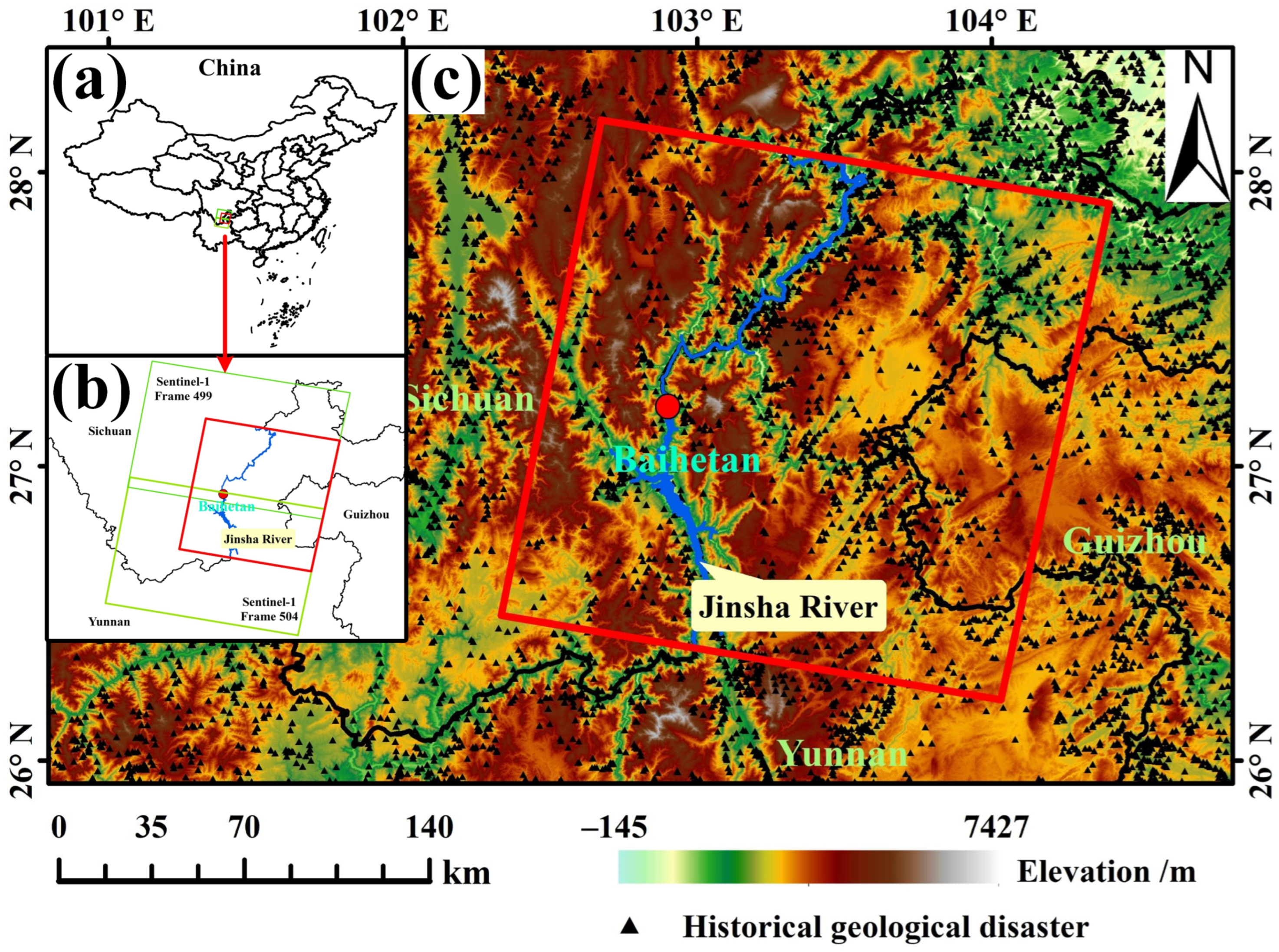
2.1. Study Area
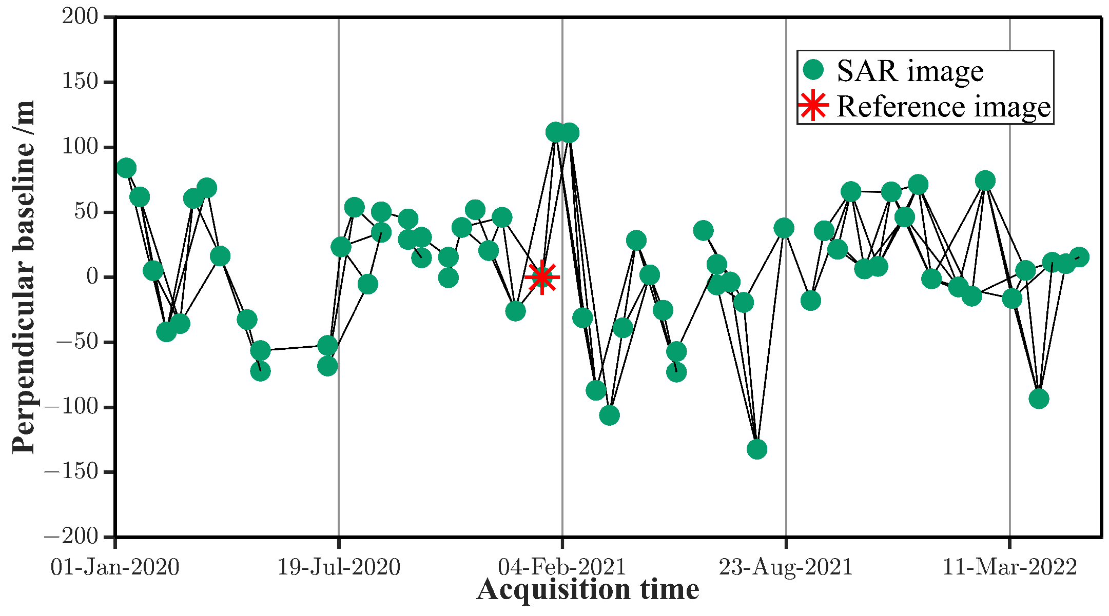
2.2. Datasets
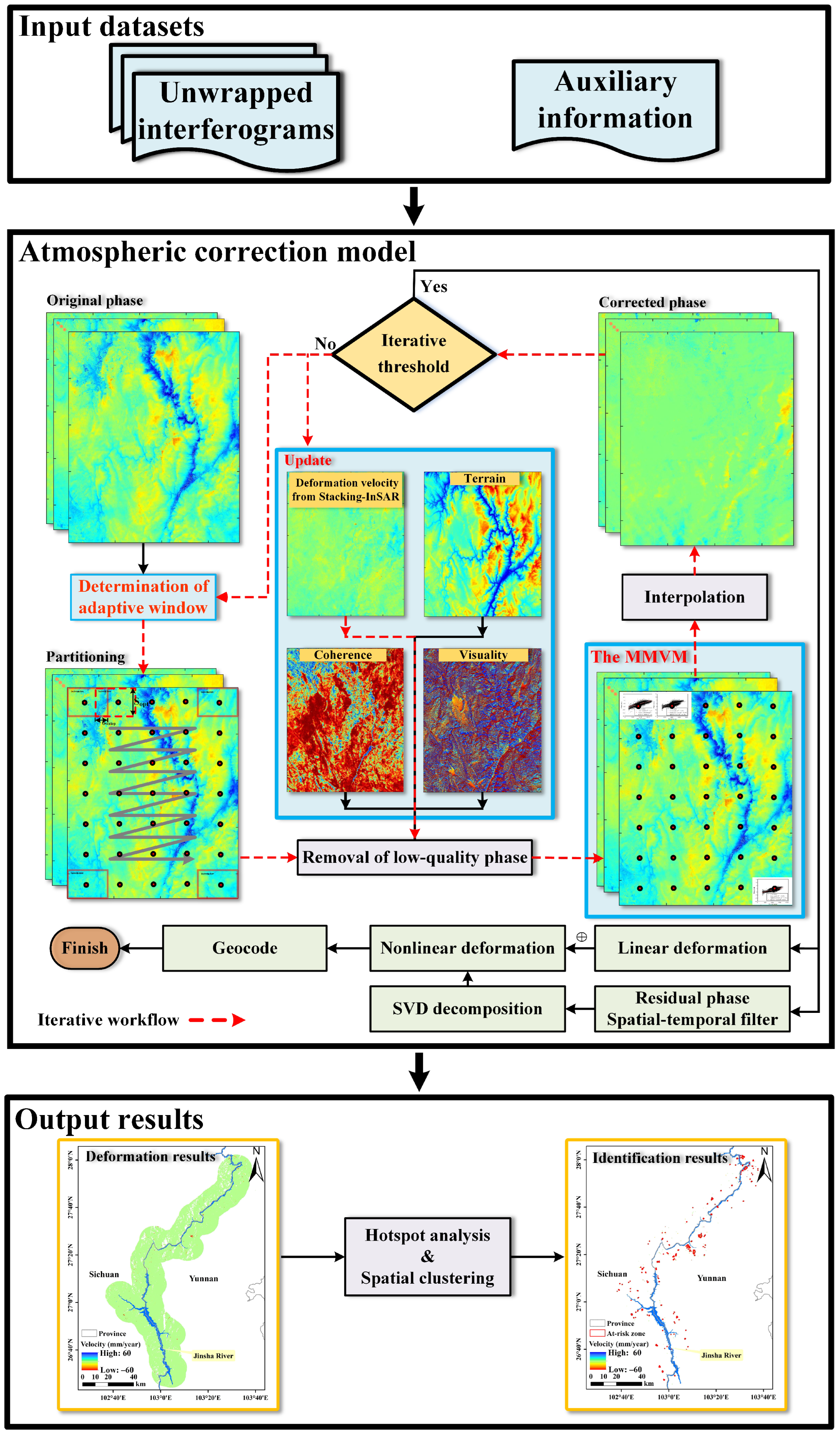
3. Methodology
3.1. InSAR Processing
3.1.1. SBAS-InSAR Processing
3.1.2. Stacking-InSAR Processing
3.2. Improved Tropospheric Delay Correction Method
3.2.1. Adaptive Window Selection
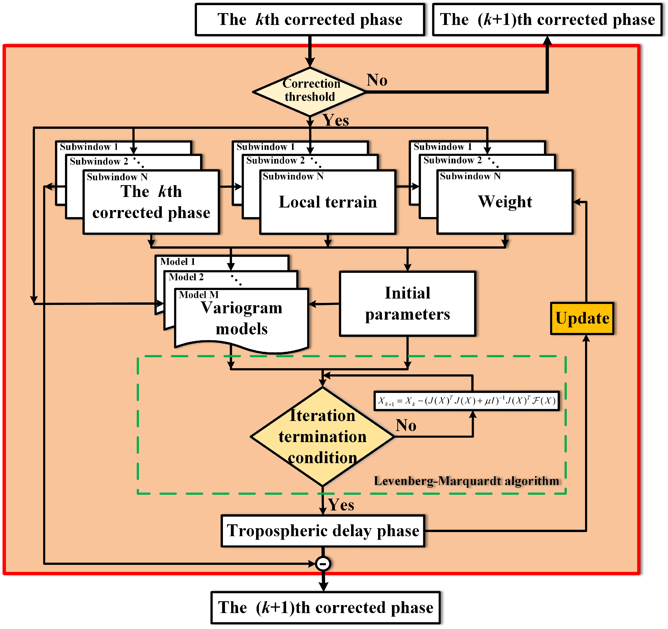
3.2.2. The MMVM-Based Tropospheric Delay Correction Method
3.3. Hotspot Analysis and Spatial Clustering
4. Results
5. Discussion
5.1. Performance Evaluation of MMVM-Based Correction Method
5.1.1. Statistical Evaluation of Corrected Interferograms
5.1.2. Improvement in Derived Deformation Rate
5.1.3. Stability of Time-Series Deformation
5.2. Advantages and Limitations of the Proposed Method
6. Conclusions
Author Contributions
Funding
Institutional Review Board Statement
Informed Consent Statement
Data Availability Statement
Acknowledgments
Conflicts of Interest
References
- Varnes, D.; David, J. Slope movement types and processes. Transp. Res. Board Spec. Rep. 1978, 176, 11–33. [Google Scholar]
- Luo, S.; Feng, G.; Xiong, Z.; Wang, H.; Zhao, Y.; Li, K.; Deng, K.; Wang, Y. An Improved Method for Automatic Identification and Assessment of Potential Geohazards Based on MT-InSAR Measurements. Remote Sens. 2021, 13, 3490. [Google Scholar] [CrossRef]
- Ran, P.; Li, S.; Zhuo, G.; Wang, X.; Meng, M.; Liu, L.; Chen, Y.; Huang, H.; Ye, Y.; Lei, X. Early Identification and Influencing Factors Analysis of Active Landslides in Mountainous Areas of Southwest China Using SBAS-InSAR. Sustainability 2023, 15, 4366. [Google Scholar] [CrossRef]
- Zhu, K.; Xu, P.; Cao, C.; Zheng, L.; Liu, Y.; Dong, X. Preliminary Identification of Geological Hazards from Songpinggou to Feihong in Mao County along the Minjiang River Using SBAS-InSAR Technique Integrated Multiple Spatial Analysis Methods. Sustainability 2021, 13, 1017. [Google Scholar] [CrossRef]
- Notti, D.; Davalillo, J.C.; Herrera, G.; Mora, O. Assessment of the performance of X-band satellite radar data for landslide mapping and monitoring: Upper Tena Valley case study. Nat. Hazards Earth Syst. Sci. 2010, 10, 1865–1875. [Google Scholar] [CrossRef]
- Ren, T.; Gong, W.; Bowa, V.; Tang, H.; Chen, J.; Zhao, F. An Improved R-Index Model for Terrain Visibility Analysis for Landslide Monitoring with InSAR. Remote Sens. 2021, 13, 1938. [Google Scholar] [CrossRef]
- Fournier, T.; Pritchard, M.; Finnegan, N. Accounting for Atmospheric Delays in InSAR Data in a Search for Long-Wavelength Deformation in South America. IEEE Trans. Geosci. Remote Sens. 2011, 49, 3856–3867. [Google Scholar] [CrossRef]
- Ferretti, A.; Prati, C. Nonlinear subsidence rate estimation using permanent scatterers in differential SAR interferometry. IEEE Trans. Geosci. Remote Sens. 2000, 38, 2202–2212. [Google Scholar] [CrossRef]
- Berardino, P.; Fornaro, G.; Lanari, R.; Sansosti, E. A new algorithm for surface deformation monitoring based on small baseline differential SAR interferograms. IEEE Trans. Geosci. Remote Sens. 2002, 40, 2375–2383. [Google Scholar] [CrossRef]
- Su, Y.; Yang, H.; Peng, J.; Liu, Y.; Zhao, B.; Shi, M. A Novel Near-Real-Time GB-InSAR Slope Deformation Monitoring Method. Remote Sens. 2022, 14, 5585. [Google Scholar] [CrossRef]
- Liao, M.; Jiang, H.; Wang, Y.; Wang, T.; Zhang, L. Improved topographic mapping through high-resolution SAR interferometry with atmospheric effect removal. ISPRS J. Photogramm. 2013, 80, 72–79. [Google Scholar] [CrossRef]
- Zhang, X.; Li, Z.; Liu, Z. Reduction of Atmospheric Effects on InSAR Observations through Incorporation of GACOS and PCA Into Small Baseline Subset InSAR. IEEE Trans. Geosci. Remote Sens. 2023, 61, 5209115. [Google Scholar] [CrossRef]
- Zhao, Y.; Zuo, X.; Li, Y.; Guo, S.; Bu, J.; Yang, Q. Evaluation of InSAR Tropospheric Delay Correction Methods in a Low-Latitude Alpine Canyon Region. Remote Sens. 2023, 15, 990. [Google Scholar] [CrossRef]
- Tymofyeyeva, E.; Fialko, Y. Mitigation of atmospheric phase delays in InSAR data, with application to the eastern California shear zone. J. Geophys. Res. Solid Earth. 2015, 120, 5952–5963. [Google Scholar] [CrossRef]
- Darvishi, M.; Cuozzo, G.; Bruzzone, L.; Nilfouroushan, F. Performance Evaluation of Phase and Weather-Based Models in Atmospheric Correction with Sentinel-1 Data: Corvara Landslide in the Alps. IEEE J. Sel. Top. Appl. Earth Observ. Remote Sens. 2020, 13, 1332–1346. [Google Scholar] [CrossRef]
- Liang, H.; Zhang, L.; Lu, Z.; Li, X. Correction of spatially varying stratified atmospheric delays in multitemporal InSAR. Remote Sens. Environ. 2023, 285. [Google Scholar] [CrossRef]
- Liu, Q.; Zeng, Q.; Zhang, Z. Evaluation of InSAR Tropospheric Correction by Using Efficient WRF Simulation with ERA5 for Initialization. Remote Sens. 2023, 15, 273. [Google Scholar] [CrossRef]
- Owerko, T.; Kuras, P.; Ortyl, Ł. Atmospheric Correction Thresholds for Ground-Based Radar Interferometry Deformation Monitoring Estimated Using Time Series Analyses. Remote Sens. 2020, 12, 2236. [Google Scholar] [CrossRef]
- Chen, Y.; Li, Z.; Penna, N. Interferometric synthetic aperture radar atmospheric correction using a GPS-based iterative tropospheric decomposition model. Remote Sens. Environ. 2018, 204, 109–121. [Google Scholar] [CrossRef]
- Xiao, R.; Yu, C.; Li, Z.; He, X. Statistical assessment metrics for InSAR atmospheric correction: Applications to generic atmospheric correction online service for InSAR (GACOS) in Eastern China. Int. J. Appl. Earth Obs. Geoinf. 2021, 96, 102289. [Google Scholar] [CrossRef]
- Karanam, V.; Mahdi, M.; Shagun, G.; Kamal, J. Multi-sensor remote sensing analysis of coal fire induced land subsidence in Jharia Coalfields, Jharkhand, India. Int. J. Appl. Earth Obs. Geoinf. 2021, 102, 102439. [Google Scholar] [CrossRef]
- Onn, F. Correction for interferometric synthetic aperture radar atmospheric phase artifacts using time series of zenith wet delay observations from a GPS network. Geophys. Res. Solid Earth. 2006, 111, B09102. [Google Scholar] [CrossRef]
- Bekaert, D.; Hooper, A.; Wright, T. A spatially variable power law tropospheric correction technique for InSAR data. Geophys. Res. Solid Earth. 2015, 120, 1345–1356. [Google Scholar] [CrossRef]
- Chen, Y.; Li, Z.; Penna, N. Triggered afterslip on the southern Hikurangi subduction interface following the 2016 Kaikura earthquake from InSAR time series with atmospheric corrections. Remote Sens. Environ. 2020, 251, 112097. [Google Scholar] [CrossRef]
- Kinoshita, Y. Development of InSAR Neutral Atmospheric Delay Correction Model by Use of GNSS ZTD and Its Horizontal Gradient. IEEE Trans. Geosci. Remote Sens. 2022, 60, 5231414. [Google Scholar] [CrossRef]
- Liang, H.; Zhang, L.; Ding, X.; Lu, Z.; Li, X. Toward Mitigating Stratified Tropospheric Delays in Multitemporal InSAR: A Quadtree Aided Joint Model. IEEE Trans. Geosci. Remote Sens. 2019, 57, 291–303. [Google Scholar] [CrossRef]
- Wang, Y.; Dong, J.; Zhang, L.; Zhang, L.; Deng, S.; Zhang, G.; Liao, M.; Gong, J. Refined InSAR tropospheric delay correction for wide-area landslide identification and monitoring. Remote Sens. Environ. 2022, 275, 113013. [Google Scholar] [CrossRef]
- Shi, M.; Peng, J.; Chen, X.; Zheng, Y.; Yang, H.; Su, Y.; Wang, G.; Wang, W. An Improved Method for InSAR Atmospheric Phase Correction in Mountainous Areas. IEEE J. Sel. Top. Appl. Earth Observ. Remote Sens. 2021, 14, 10509–10519. [Google Scholar] [CrossRef]
- Barnhart, W.; Lohman, R. Characterizing and estimating noise in InSAR and InSAR time series with MODIS. Geochem. Geophys. Geosyst. 2013, 14, 4121–4132. [Google Scholar] [CrossRef]
- Bekaert, D.; Walters, R.; Wright, T.; Hooper, A.; Parker, D. Statistical comparison of InSAR tropospheric correction techniques. Remote Sens. Environ. 2015, 170, 40–47. [Google Scholar] [CrossRef]
- Cavalié, O.; Doin, M.; Lasserre, C.; Briole, P. Ground motion measurement in the Lake Mead area, Nevada, by differential synthetic aperture radar interferometry time series analysis: Probing the lithosphere rheological structure. J. Geophys. Res. Solid Earth. 2007, 112, B03403. [Google Scholar] [CrossRef]
- Delacourt, C.; Briole, P.; Achache, J. Tropospheric corrections of SAR interferograms with strong topography. Application to Etna. Geophys. Res. Lett. 1998, 25, 2849–2852. [Google Scholar] [CrossRef]
- Lin, Y.; Simons, M.; Hetland, E.; Muse, P.; DiCaprio, C. A multiscale approach to estimating topographically correlated propagation delays in radar interferograms. Geochem. Geophys. Geosyst. 2010, 11, 9. [Google Scholar] [CrossRef]
- Li, Z.; Cao, Y.; Wei, J.; Duan, M.; Wu, L.; Hou, J.; Zhu, J. Time-series InSAR ground deformation monitoring: Atmospheric delay modeling and estimating. Earth-Sci. Rev. 2019, 192, 258–284. [Google Scholar] [CrossRef]
- Lu, P.; Casagli, N.; Catani, F.; Tofani, V. Persistent scatterers interferometry hotspot and cluster analysis (PSI-HCA) for detection of extremely slow-moving landslides. Int. J. Remote Sens. 2012, 33, 466–489. [Google Scholar] [CrossRef]
- Dai, H.; Zhang, H.; Dai, H.; Wang, C.; Tang, W.; Zou, L.; Tang, Y. Landslide Identification and Gradation Method Based on Statistical Analysis and Spatial Cluster Analysis. Remote Sens. 2022, 14, 4504. [Google Scholar] [CrossRef]
- Ni, W.; Zhao, L.; Zhang, L.; Xing, K.; Dou, J. Coupling Progressive Deep Learning with the AdaBoost Framework for Landslide Displacement Rate Prediction in the Baihetan Dam Reservoir, China. Remote Sens. 2023, 15, 2296. [Google Scholar] [CrossRef]
- Liu, H.; Luo, Y.; Feng, W.; Wang, Y.; Ma, H.; Hu, P. Site response of ancient landslides to initial impoundment of Baihetan Reservoir (China) based on ambient noise investigation. Soil Dyn. Eearthq. Eng. 2023, 167, 107590. [Google Scholar] [CrossRef]
- Cheng, Z.; Liu, S.; Fan, X.; Shi, A.; Yin, K. Deformation behavior and triggering mechanism of the Tuandigou landslide around the reservoir area of Baihetan hydropower station. Landslides 2023, 20, 1679–1689. [Google Scholar] [CrossRef]
- Yi, X.; Feng, W.; Li, B.; Yin, B.; Dong, X.; Xin, C.; Wu, M. Deformation characteristics, mechanisms, and potential impulse wave assessment of the Wulipo landslide in the Baihetan reservoir region, China. Landslides 2023, 20, 615–628. [Google Scholar] [CrossRef]
- Liu, M.; Yang, Z.; Xi, W.; Guo, J.; Yang, H. InSAR-based method for deformation monitoring of landslide source area in Baihetan reservoir, China. Front. Earth Sci. 2023, 11, 1253272. [Google Scholar] [CrossRef]
- Dun, J.; Feng, W.; Yi, X.; Zhang, G.; Wu, M. Detection and Mapping of Active Landslides before Impoundment in the Baihetan Reservoir Area (China) Based on the Time-Series InSAR Method. Remote Sens. 2021, 13, 3213. [Google Scholar] [CrossRef]
- Karabork, H.; Makineci, H.; Orhan, O.; Karakus, P. Accuracy assessment of DEMs derived from multiple SAR data using the InSAR technique. Arab. J. Sci. Eng. 2021, 46, 5755–5765. [Google Scholar] [CrossRef]
- Xu, Y.; Li, T.; Tang, X.; Zhang, X.; Fan, H.; Wang, Y. Research on the Applicability of DInSAR, Stacking-InSAR and SBAS-InSAR for Mining Region Subsidence Detection in the Datong Coalfield. Remote Sens. 2022, 14, 3314. [Google Scholar] [CrossRef]
- Li, Y.; Zhang, J.; Li, Z.; Luo, Y.; Jiang, W.; Tian, Y. Measurement of subsidence in the Yangbajing geothermal fields, Tibet, from TerraSAR-X InSAR time series analysis. Int. J. Digit. Earth. 2016, 9, 697–709. [Google Scholar] [CrossRef]
- Xiao, R.; Yu, C.; Li, Z.; Jiang, M.; He, X. InSAR stacking with atmospheric correction for rapid geohazard detection: Applications to ground subsidence and landslides in China. Int. J. Appl. Earth Obs. Geoinf. 2022, 115, 103082. [Google Scholar] [CrossRef]
- Jia, H.; Wang, Y.; Ge, D.; Deng, Y.; Wang, R. InSAR Study of Landslides: Early Detection, Three-Dimensional, and Long-Term Surface Displacement Estimation-A Case of Xiaojiang River Basin, China. Remote Sens. 2022, 14, 1759. [Google Scholar] [CrossRef]
- Zhang, B.; Hestir, E.; Yunjun, Z.; Reiter, M.; Viers, J.; Schaffer-Smith, D.; Sesser, K.; Oliver-Cabrera, T. Automated Reference Points Selection for InSAR Time Series Analysis on Segmented Wetlands. IEEE Geosci. Remote Sens. Lett. 2024, 21, 4008705. [Google Scholar] [CrossRef]
- Bekaert, D.; Handwerger, A.; Agram, P.; Kirschbaum, D. InSAR-based detection method for mapping and monitoring slow-moving landslides in remote regions with steep and mountainous terrain: An application to Nepal. Remote Sens. Environ. 2020, 249, 111983. [Google Scholar] [CrossRef]
- Zhang, G.; Xu, Z.; Chen, Z.; Wang, S.; Cui, H.; Zheng, Y. Predictable Condition Analysis and Prediction Method of SBAS-InSAR Coal Mining Subsidence. IEEE Trans. Geosci. Remote Sens. 2022, 60, 5232914. [Google Scholar] [CrossRef]
- Chen, Z.; White, L.; Banks, S.; Behnamian, A.; Montpetit, B.; Pasher, J.; Duffe, J.; Bernard, D. Characterizing marsh wetlands in the Great Lakes Basin with C-band InSAR observations. Remote Sens. Environ. 2020, 242, 111750. [Google Scholar] [CrossRef]
- Hu, Z.; Mallorquí, J. An Accurate Method to Correct Atmospheric Phase Delay for InSAR with the ERA5 Global Atmospheric Model. Remote Sens. 2019, 11, 1969. [Google Scholar] [CrossRef]
- Yu, C.; Li, Z.; Penna, N.; Crippa, P. Generic atmospheric correction model for interferometric synthetic aperture radar observations. J. Geophys. Res. Solid Earth 2018, 123, 9202–9222. [Google Scholar] [CrossRef]


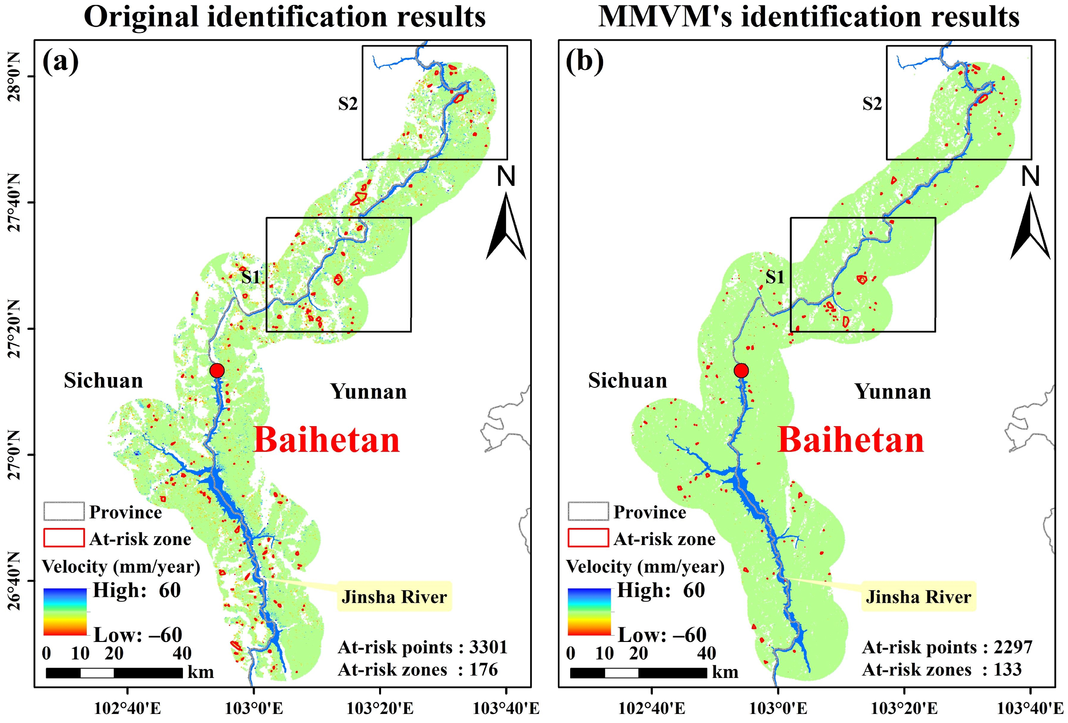
| Method | At-Risk Points | At-Risk Zones | Accuracy |
|---|---|---|---|
| Original | 3301 | 176 | 47.159% |
| After Correction | 2297 | 133 | 96.241% |
| No. | Name | Longitude | Latitude | Area | Maximum Rate | Maximum Deformation | Aspect | Threat Object |
|---|---|---|---|---|---|---|---|---|
| (°) | (°) | (km2) | (mm/year) | (mm) | ||||
| 1 | Luotianba | 103.58 | 27.98 | 0.031 | −24.098 | −36.274 | W | River, villages |
| 2 | Sunjialiangzi | 103.59 | 27.94 | 0.017 | −28.744 | −40.041 | SW | Villages, roads |
| 3 | Lijiaping | 103.52 | 27.93 | 0.168 | −25.042 | −57.358 | NW | Villages, river, and roads |
| 4 | Wozitou | 103.52 | 27.71 | 0.039 | −57.750 | −113.923 | W | Villages, farmlands, and roads |
| 5 | Qianligou | 103.32 | 27.69 | 0.022 | −24.243 | −34.381 | S | Villages, farmlands, and roads |
| 6 | Gongshan | 103.24 | 27.59 | 0.055 | −27.401 | −48.558 | SW | Villages, farmlands |
| 7 | Liangshanjing | 103.23 | 27.48 | 0.025 | −41.725 | −75.183 | SW | Villages, farmlands |
| 8 | Yujiapingzi | 103.25 | 27.46 | 0.022 | −25.286 | −66.031 | W | Villages, farmlands, and roads |
| 9 | Dayadong | 103.25 | 27.40 | 0.032 | −26.053 | −38.562 | S | Villages, roads |
| 10 | Galuo | 102.95 | 27.45 | 0.336 | −31.396 | −54.545 | W | Villages, roads |
| 11 | Shanshu | 103.25 | 27.38 | 0.001 | −29.191 | −58.825 | S | Villages, roads |
| 12 | Niupingyan | 103.12 | 27.39 | 0.034 | −35.932 | −72.767 | SW | Villages, roads |
| 13 | Ertun | 103.00 | 27.40 | 0.098 | −32.063 | −72.047 | SE | Villages, roads |
| 14 | Youyicun | 102.85 | 27.14 | 0.130 | −34.710 | −51.933 | SE | Villages, farmlands |
| 15 | Huodi | 103.06 | 26.90 | 0.570 | −30.339 | −52.472 | SW | Villages, farmlands |
| 16 | Xintian | 103.12 | 26.67 | 0.015 | −22.794 | −48.206 | E | River, villages |
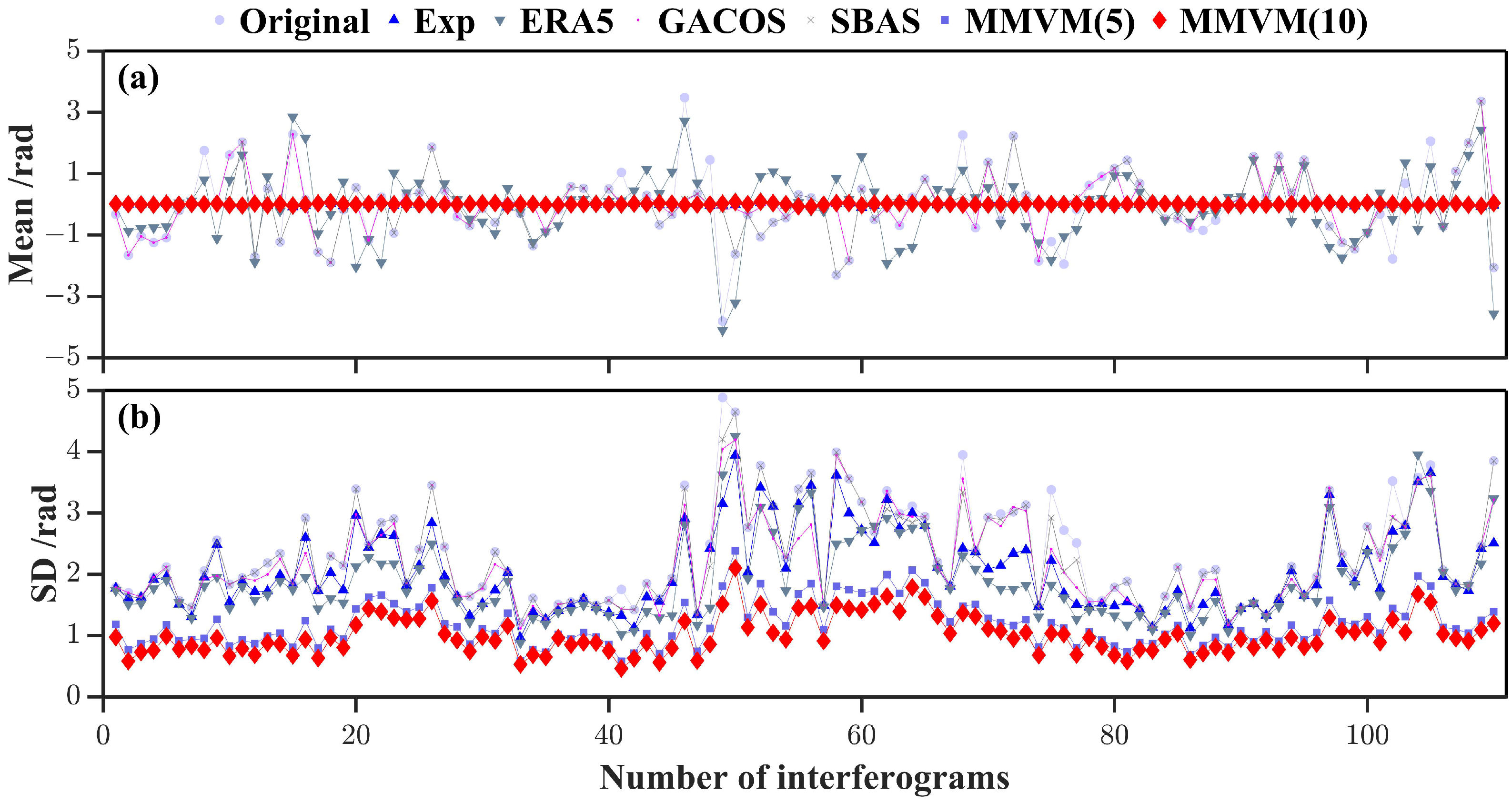
| Method | Number with Reduced SD | SD (rad) | Number with Mean Closer to 0 | Mean (rad) |
|---|---|---|---|---|
| Original | 110 | 2.3228 | 110 | −0.0327 |
| Exp | 110 | 2.0449 | 106 | 0.0101 |
| ERA5 | 107 | 1.8854 | 61 | −0.0606 |
| GACOS | 43 | 2.1990 | 42 | 0.0326 |
| SBAS | 39 | 2.2711 | 36 | 0.0103 |
| MMVM(5) | 110 | 1.1893 | 106 | 0.0040 |
| MMVM(10) | 110 | 1.0123 | 107 | 0.0045 |
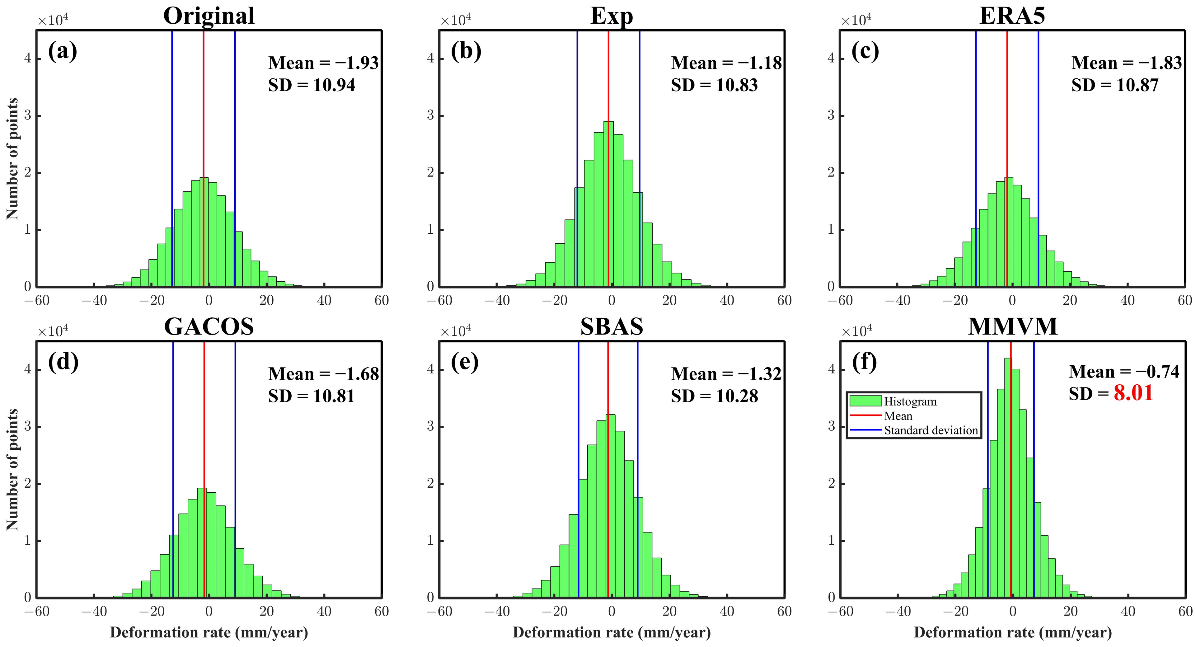
| Method | MPs | Non-Deformed Area | Deformed Area | ||
|---|---|---|---|---|---|
| MPs | SD | Mean | SD | ||
| (mm/year) | (mm/year) | (mm/year) | |||
| Original | 173,349 | 61,530 | 2.8320 | −2.9009 | 13.3601 |
| Exp | 218,352 | 81,333 | 2.8310 | −1.8157 | 13.4583 |
| ERA5 | 170,706 | 62,201 | 2.8274 | −2.7907 | 13.3704 |
| GACOS | 152,046 | 56,331 | 2.8346 | −2.5942 | 13.3697 |
| SBAS | 245,442 | 95,205 | 2.8307 | −2.0812 | 12.8820 |
| MMVM | 296,813 | 150,071 | 2.7633 | −1.3111 | 11.0191 |
| Method | Non-Deformed Areas | Deformed Areas | ||
|---|---|---|---|---|
| MPs | SD | Mean | SD | |
| (mm/year) | (mm/year) | (mm/year) | ||
| Original | 4,329,987 | 0.6469 | −0.0020 | 2.5300 |
| Exp | 5,601,942 | 0.6464 | −0.0248 | 3.3740 |
| ERA5 | 4,772,330 | 0.6444 | 0.0006 | 2.3842 |
| GACOS | 4,657,488 | 0.6478 | 0.0054 | 2.8266 |
| SBAS | 4,644,076 | 0.6464 | −0.0017 | 2.5607 |
| MMVM | 8,897,582 | 0.6236 | −0.0482 | 2.4970 |
| Method | Non-Deformed Areas | Deformed Areas | ||
|---|---|---|---|---|
| MPs | SD | Mean | SD | |
| (mm/year) | (mm/year) | (mm/year) | ||
| Original | 98,255 | 0.6431 | 0.0008 | 2.2065 |
| Exp | 107,778 | 0.6426 | −0.0004 | 2.7814 |
| ERA5 | 118,150 | 0.6374 | 0.0007 | 2.0490 |
| GACOS | 86,101 | 0.6347 | 0.0011 | 2.4283 |
| SBAS | 97,495 | 0.6443 | 0.0008 | 2.2063 |
| MMVM | 179,376 | 0.5882 | −0.0005 | 1.7713 |
| Method | Standard Deviation from Fit | |
|---|---|---|
| FP1 (mm) | FP2 (mm) | |
| Original | 6.278 | 4.213 |
| Exp | 5.965 | 4.267 |
| ERA5 | 6.259 | 4.321 |
| GACOS | 6.303 | 4.863 |
| SBAS | 6.684 | 5.306 |
| MMVM | 4.773 | 3.022 |
| Method | Plain | Steep Terrain | Computational Efficiency | External Data | Advantages | Disadvantages |
|---|---|---|---|---|---|---|
| Exp | Good | Good | Medium | No | Satisfies the spatial heterogeneity | Sensitive to deformed or turbulent signals, small-scale |
| ERA5 | Good | Poor | Low | Yes | Wide-scale | Uncertainty in estimated tropospheric delay phases |
| GACOS | Good | Poor | Medium | Yes | Wide-scale | Uncertainty in estimated tropospheric delay phases |
| SBAS | Good | Good | High | No | Various monitoring scenarios | Unable to satisfy the spatial heterogeneity |
| MMVM | Excellent | Excellent | Low | No | Wide-scale, various monitoring scenarios, and satisfies the spatial heterogeneity | Phase overcorrection in some areas |
Disclaimer/Publisher’s Note: The statements, opinions and data contained in all publications are solely those of the individual author(s) and contributor(s) and not of MDPI and/or the editor(s). MDPI and/or the editor(s) disclaim responsibility for any injury to people or property resulting from any ideas, methods, instructions or products referred to in the content. |
© 2024 by the authors. Licensee MDPI, Basel, Switzerland. This article is an open access article distributed under the terms and conditions of the Creative Commons Attribution (CC BY) license (https://creativecommons.org/licenses/by/4.0/).
Share and Cite
Li, L.; Wang, J.; Zhang, H.; Zhang, Y.; Xiang, W.; Fu, Y. Refined InSAR Mapping Based on Improved Tropospheric Delay Correction Method for Automatic Identification of Wide-Area Potential Landslides. Remote Sens. 2024, 16, 2187. https://doi.org/10.3390/rs16122187
Li L, Wang J, Zhang H, Zhang Y, Xiang W, Fu Y. Refined InSAR Mapping Based on Improved Tropospheric Delay Correction Method for Automatic Identification of Wide-Area Potential Landslides. Remote Sensing. 2024; 16(12):2187. https://doi.org/10.3390/rs16122187
Chicago/Turabian StyleLi, Lu, Jili Wang, Heng Zhang, Yi Zhang, Wei Xiang, and Yuanzhao Fu. 2024. "Refined InSAR Mapping Based on Improved Tropospheric Delay Correction Method for Automatic Identification of Wide-Area Potential Landslides" Remote Sensing 16, no. 12: 2187. https://doi.org/10.3390/rs16122187