Abstract
In an increasingly globalized world, the intelligent extraction of maritime targets is crucial for both military defense and maritime traffic monitoring. The flexibility and cost-effectiveness of unmanned aerial vehicles (UAVs) in remote sensing make them invaluable tools for ship extraction. Therefore, this paper introduces a training-free, highly accurate, and stable method for ship extraction in UAV remote sensing images. First, we present the dynamic tracking matched filter (DTMF), which leverages the concept of time as a tuning factor to enhance the traditional matched filter (MF). This refinement gives DTMF superior adaptability and consistent detection performance across different time points. Next, the DTMF method is rigorously integrated into a recurrent neural network (RNN) framework using mathematical derivation and optimization principles. To further improve the convergence and robust of the RNN solution, we design an adaptive feedback recurrent neural network (AFRNN), which optimally solves the DTMF problem. Finally, we evaluate the performance of different methods based on ship extraction accuracy using specific evaluation metrics. The results show that the proposed methods achieve over 99% overall accuracy and KAPPA coefficients above 82% in various scenarios. This approach excels in complex scenes with multiple targets and background interference, delivering distinct and precise extraction results while minimizing errors. The efficacy of the DTMF method in extracting ship targets was validated through rigorous testing.
1. Introduction
In today’s globalized world, maritime ship detection is crucial for national defense, military security [1], and maritime traffic monitoring [2]. First and foremost, real-time surveillance of vast sea areas is essential to identify and track potential maritime threats, such as enemy ships, submarines, or other suspicious vessels. This vigilance plays a critical role in safeguarding national maritime security and sovereignty [3]. Moreover, as maritime routes grow increasingly congested due to the expansion of global trade [4], an effective ship monitoring system is imperative to prevent accidents like collisions and groundings, ensuring safe navigation [5].
In this context, unmanned aerial vehicle (UAV) remote sensing technology has emerged as a powerful tool for enhancing military defense and maritime traffic planning [6,7]. UAV remote sensing, with its high flexibility and low operational costs [8], complements satellite remote sensing by providing localized and high-resolution data. While UAVs can be rapidly deployed in a variety of weather conditions, their effectiveness may be limited under severe weather circumstances such as high winds. Despite this, they remain particularly valuable for swift emergency response under most operational environments [9]. Unlike traditional satellite or airborne remote sensing, UAVs can adjust flight paths and altitudes flexibly, focusing on specific areas, particularly those with challenging or inaccessible geography. Moreover, UAVs deliver near real-time data crucial for swift decision-making and response in search and rescue operations or environmental monitoring. Modern UAVs often come equipped with advanced data processing systems that can analyze images mid-flight, offering real-time insights [10,11,12]. Furthermore, UAVs can capture targets from various angles and altitudes [13], improving the accuracy of ship identification and surveillance. This study aims to propose a fast and accurate ship identification method for effective monitoring. Typically, researchers rely on two primary techniques for ship extraction: traditional target detection from remote sensing images and deep learning approaches.
Remote sensing target extraction is fundamentally a binary classification problem, with its primary objective being the effective separation of the object of interest from the complex background [14,15]. Given the widespread acquisition and application of remote sensing images, numerous classical target detection algorithms have been developed and widely applied in recent decades. These algorithms are designed to minimize the interference of background information while enhancing the expression of target features, thus making targets more prominent and easier to detect in complex environments. Some of the representative algorithms include the match filter (MF) [16,17], adaptive coherence estimator (ACE) [18,19], and constrained energy minimization (CEM) [20,21]. Stephanie et al. [22] describe the ACE algorithm as a generalized likelihood ratio test (GLRT) within a homogeneous setting, where the covariance matrix of the auxiliary data is proportional to that of the measured vectors. The MF approach resembles ACE by treating target detection as a hypothesis-testing problem, assuming that targets and backgrounds follow different probability models. Through GLRT, MF effectively distinguishes targets from their background. This statistical target detection technique relies on the accurate differentiation of target and background probability distributions for successful identification. In practice, MF usually leverages local statistical information through a double-window technique to gather accurate statistics of the surrounding background. The CEM method proposed by William et al. [23] seeks to maximize the spectral response of the target while suppressing the background response, enabling effective separation between them. The CEM method employs a finite impulse response (FIR) detector to minimize the energy across the image while maintaining a fixed target spectral response value.
Although classical remote sensing target extraction methods have yielded positive results across various fields, the complexity and variability of real-world application scenarios necessitate further refinement. Many researchers have worked to improve traditional methods to enhance detection accuracy in different contexts. Various strategies have been proposed to better tailor target detection methods to specific environmental needs. Xiong et al. [24] combined the CEM method with a neural dynamics algorithm to extract Arctic sea ice from remote sensing images, demonstrating its efficacy in noisy environments. Shuo et al. [25] introduced an algorithm that integrates sparsity with both CEM and ACE. Similarly, Chen et al. [26] developed a noise-resistant matched filter scheme using Newton’s algorithm to identify islands and reefs. In a related study, Chaillan et al. [27] proposed a stochastic matched filter for synthetic aperture radar (SAR) image wake monitoring, using a discrete Radon transform to detect straight-line patterns. This technique is followed by a stochastic matched filter that enhances the signal-to-noise ratio of the observation. Despite these improvements, these methods lack spatial and dynamic information regarding the underlying optimization problems, resulting in suboptimal performance for ship extraction tasks. Moreover, current UAV remote sensing ship extraction techniques still have significant room for enhancement. Optimizing pixel-oriented remote sensing feature detection algorithms remains challenging, especially with phenomena like “homospectral–heterospectral”, affecting feature extraction.
In recent years, deep learning has gained popularity and has been applied across numerous engineering fields. Compared to object-oriented methods, deep learning has significant advantages in feature learning, end-to-end learning, adaptability, nonlinear modeling, and handling big data, particularly for remote sensing target extraction, such as ship monitoring. Deep learning has achieved remarkable success in fields like image recognition, speech recognition, and natural language processing, becoming a central focus in AI research. Kim et al. [28] employed the Faster-R-CNN network combined with Bayesian methods for ship detection and classification, achieving an average detection accuracy of 93.92%. The S-CNN model proposed by Zhang et al. [29] addresses suboptimal detection when confronted with varied classes and sizes of ship targets. Wang et al. [30] developed GT-YOLO, an enhanced model based on YOLOv5s, incorporating a feature fusion module with an attention mechanism to improve network feature fusion. This model introduces separable convolution to enhance the detection accuracy of small targets and low-resolution images. Finally, Zhao et al. [31] proposed a Domain Adaptive (DA) Transformer target detection method to tackle challenges posed by unlabeled multi-source satellite-borne SAR images of ships.
While deep learning has achieved remarkable success in various domains, it is crucial to recognize its limitations. Deep learning models often require large amounts of labeled data, especially for complex tasks involving extensive datasets [32,33,34]. Thus, the data volume needed for optimal generalization expands significantly. Collecting substantial labeled data is a time-consuming and labor-intensive process, incurring high costs and requiring significant human resources [35,36,37]. Moreover, when training data are limited or the model complexity is excessive, deep learning models are prone to overfitting [38,39]. This occurs when the model performs well on the training data but its performance deteriorates with unseen data, impairing its predictive capacity. Additionally, the opaque nature of deep learning models makes it challenging to understand their decision-making processes and how features are extracted. This lack of transparency is particularly problematic in sensitive fields such as medical diagnosis and legal decision-making. Furthermore, the training and inference processes of deep learning models require significant computational resources, particularly for deep models with extensive datasets. These models rely heavily on advanced computational hardware and sufficient resources to function effectively. Consequently, training complex deep learning models with limited resources can be time-consuming and inefficient, posing a challenge for applications that require rapid and accurate ship monitoring and extraction from remote sensing imagery.
Meanwhile, recurrent neural networks (RNNs) [40,41,42,43,44] have gained popularity due to their efficiency and robustness in solving real-time problems. However, existing RNN models are fundamentally designed for dynamic control and optimization tasks, making them less suitable for remote sensing target extraction. Additionally, the activation function [45] is a critical component affecting the convergence speed and accuracy of RNN models. Despite its importance, few studies have focused on developing specialized activation functions to improve RNN performance in remote sensing target extraction.
This paper proposes a dynamic tracking matched filter (DTMF) scheme for the extraction of ships from UAV remote sensing images. DTMF incorporates a dynamic penalty term based on the MF and combines the dynamic adjustments of the regularization parameter and the time variable to strengthen the orientation towards satisfying the constraints. Furthermore, the time variable is introduced as a reconciliation factor, whereby the regularization parameter grows exponentially with time, adapting to the dynamic changes in the system. This ensures that the algorithm accurately tracks the target spectral vectors over time, and is able to have good adaptability and sustained detection performance at different time points. Subsequently, DTMF is integrated into the RNN solution framework through a rigorous mathematical derivation. In order to enhance the resilience and precision of the detection scheme, a novel nonlinear activation function is introduced and an AFRNN model that can be dynamically calibrated to adapt to fluctuations in the input data or environmental conditions is proposed. This model eliminates the time lag problem and facilitates rapid convergence. In addition, a systematic theoretical analysis and corresponding results of the AFRNN model are presented to investigate and ensure its convergence and robustness. The technical route of this paper is shown in Figure 1.
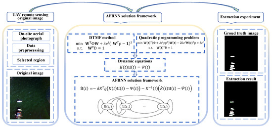
Figure 1.
Technical line.
This paper is divided into five sections. The initial section of the paper presents a summary of the current state of research in the field of remote sensing target extraction and RNN methods, along with an analysis of their respective limitations. This serves to establish a foundation for the proposed method. The second part of the paper proposes the DTMF method and transforms it into a dynamic system of equations in order to prepare for the subsequent solution. The third part incorporates the DTMF dynamic equation set into the RNN solving framework and proposes an AFRNN model for solving. Subsequently, the proposed AFRNN model is subjected to comprehensive algorithmic analysis and some theorem proofs are provided to demonstrate the algorithm’s feasibility. The fourth part compares the visualization results of the proposed DTMF ship target extraction method with those of the traditional remote sensing target extraction method. It discusses the advantages and disadvantages of the different algorithms and verifies the superiority of this paper’s method. The principal contributions of this paper are as follows:
- A novel DTMF ship target extraction model is proposed. DTMF introduces dynamic penalty terms based on MF, combining the dynamic adjustment of regularization parameters and time variables to enhance the orientation towards satisfying the constraints. Furthermore, the time variable is introduced as a reconciliation factor, whereby the regularization parameter grows exponentially with time, adapting to the dynamic changes in the system. This ensures that the algorithm accurately tracks the target spectral vectors over time, and is able to demonstrate good adaptability and sustained detection performance at different time points;
- From the control point of view, this paper proposes an AFRNN model based on RNN for solving the DTMF ship extraction method. The essence of the AFRNN model is to introduce an adaptive feedback term on the basis of the gradient RNN, and to design a special nonlinear projection function, which can be adapted to adjust dynamically according to the changes in the input data or the environment and eliminate the time lag problem;
- The efficacy of the proposed AFRNN model in addressing the DTMF method for remote sensing ship extraction is evidenced by the corresponding quantitative and visual simulation experiments and outcomes.
2. Dynamic Tracking Matched Filter
This section presents a description of the DTMF method for ship extraction. In order to facilitate the solution of the DTMF method, it is first constructed as a dynamic quadratic programming problem, which is subsequently simplified for subsequent solving.
2.1. Model Construction
In practical applications, the remote sensing image of the ship can be expressed as , where each column of the matrix belongs to space. Here, m represents the number of spectral bands, and n the number of pixels. Let be a column vector representing the spectral feature of the target. Then, the matched filter coefficients can be represented by , which is the linear operator that transforms the space. To maximize the output signal to the interference-plus-noise ratio (SINR), we need to adjust to make the output focus on the direction of the target feature vector . In this way, the output of the filter for the background clutter can be modeled as a normal distribution, where the variance . Thus, the matched filter is the optimal linear estimator that minimizes the output variance.
The coefficients of the matched filter are denoted as . Then, by reconstructing the original image using the optimal filter coefficients, we obtain the filtered output image. Finally, by applying the relevant image thresholding segmentation methods, the detection of the desired target information can be achieved. The central idea of the penalty function method is to add a penalty term to the objective function, which includes a penalty factor proportional to the degree of constraint violation. As the optimization process progresses, the method enhances the effect of the penalty term by increasing a dynamic weight factor, thereby guiding the solution towards satisfying the constraints. In this way, we can effectively solve complex constrained optimization problems. Then, by incorporating temporal information, we extend the equality-constrained matched filter in Equation (1) to a dynamic optimization:
In the optimization process, the goal is to solve the dynamic unknown vector in real time, where . The optimization objective is to minimize the objective function . The main component of the objective function, , represents the variance of the filter output signal. By minimizing this term, the effect of background noise on the filter output can be reduced. The penalty term, , is used to guide the optimization process towards a solution that satisfies the constraints. Here, is a regularization parameter that controls the weight of the penalty term in the overall objective function, and is a penalty function that measures the deviation of .
In reality, the background of remote sensing images is highly complex, and phenomena such as ’same object, different spectrum’ and ’same spectrum, different object’ frequently occur, impeding the ability to obtain the spectral vectors of the target of interest in their entirety. Consequently, the spectral vectors analogous to or similar to the target spectral vectors are obtained through sampling. The coefficient matrix is the ensemble of sampled spectral vectors, and ensures a fixed gain in the direction of the target spectral feature.
The regularization parameter balances the importance of minimizing energy with satisfying the constraints. Its size directly affects the convergence and computational efficiency of the problem. To ensure computational efficiency and convergence, it is crucial to choose appropriate penalty functions and parameters. Theoretically, under the condition that the penalty function is satisfied, the regularization parameter needs to be continuously increased during the iteration process. To achieve this, we introduce the time variable as a harmonizing factor, ensuring that the regularization parameter exponentially increases with time. This means that the system’s tolerance for error decreases over time, and as time progresses, the system increasingly ensures that the filter coefficients accurately track the target spectral vector. This dynamic adjustment is essential in systems where the spectral characteristics change over time, necessitating continuous parameter adjustments to maintain optimal performance.
To minimize algorithm complexity and save computational resources, we design the penalty function as . This squared term is continuously differentiable, and the penalty rapidly increases with the degree of deviation, imposing greater penalties on solutions that deviate further from the constraints. This ensures that the solution moves towards satisfying the constraints. Additionally, the penalty term is always non-negative, ensuring that it is always an increment to the total objective function. This maintains the bounds of the optimization function, making the optimization process more stable.
Based on the above analysis, we design the following optimization model:
This optimization model finds the optimal filter coefficients by minimizing the sum of the filter output signal variance and the penalty term. The penalty term ensures a fixed gain in the direction of the target spectral feature, allowing for target detection in a complex background. By dynamically updating the filter coefficients, this model can adapt to real-time requirements in practical applications.
2.2. Modeling Simplicity
To further expand and simplify the optimization problem, we need to extract the term . Given the term , we can use the square of a binomial formula to expand it:
we can transform the penalty termination into the following form:
First, we extract the term :
we can rewrite this as:
The optimization problem simplifies to:
We introduce the Lagrange multiplier and construct the Lagrangian function :
To solve the optimization problem, we need to take the partial derivatives of and set them to zero:
In summary, when Equation (6) is satisfied, the DTMF can obtain the optimal solution. Subsequently, to simplify the expression, the following matrix is defined:
As a result, the complex equation to be solved can be transformed into a simple linear equation as follows:
3. Adaptive Feedback Recurrent Neural Network
In the previous section, we transformed the DTMF ship target extraction model into a dynamic quadratic programming problem. The introduction of the time variable prevents this problem from being treated like a conventional static optimization problem. Therefore, traditional optimization algorithms such as the most rapid descent method and Newton’s method are not applicable in this scenario. These classical optimization methods usually rely on the information of the derivatives of the objective function to approach the optimal solution step by step, and they each have fixed accuracy limits. However, the dynamic objective function changes over time, which means that each iteration instant will face a different optimization scheme than the previous instant. The iterative approach in traditional algorithms, based on the derivative information of the moment, lacks immediate compensation for the time-varying parameters, which results in an irreparable time delay, no matter how the step size and sampling interval are set.
Based on the above problems, this section carries out the study for solving the DTMF target extraction method constructed in the previous chapter for target extraction of UAV remote sensing imagery ships.
First, we construct an error function based on the above dynamic linear Equation (7):
Based on this error function, we introduce the original zeroing neural network (OZNN) [40] and construct it as the following first-order linear differential equation:
where is a scaling parameter that adjusts the convergence speed of the linear model. Previous research has demonstrated that the dynamical system (9) can globally converge.
The Gradient Neural Network (GNN) [46] model requires the definition of an energy function based on the error and seeks the optimal solution along the negative gradient direction of the energy function. The formula for the GNN model used to solve the dynamic quadratic programming problem is as follows:
Although the GNN model (10) eliminates the need for matrix inversion, thus substantially reducing computational complexity, it incurs time delays when dealing with dynamic problems. Therefore, the GNN model (10) is not suitable for all practical application scenarios.
Remark 1.
It should be noted that is a time-varying real symmetric matrix. According to the theory of matrix diagonalization and similarity, it can be equivalent to a time-varying diagonal array. Therefore, we can obtain the following expression:
are the eigenvalues of the matrix at each moment in time. In addition, all eigenvalues satisfy the following inequality:
where and , respectively, represent the global minimum and global maximum eigenvalues of the time-symmetric matrix.
In solving the dynamic quadratic programming problem, although the GNN model (9) uses parallel computation, it lacks mechanisms to effectively cope with rapid changes in the relevant parameters, which means that there is still a gap between the solution and the theoretical solution, even at infinite time [47].
Theorem 1.
GNN model (9) allows for global convergence to a constant, which we denote as:
In the above model, the error vector norm is bounded. Specifically, ; denotes the smallest eigenvalue of .
Proof.
First, we define a Lyapunov candidate function [48]:
The time derivative of Equation (11) is:
Finally, to demonstrate the convergence properties, the GNN model Equation (9) guarantees that the is always less than or equal to . Therefore, for the final part of the proof, we can write:
Due to physical constraints, the value of cannot increase indefinitely, which leads to the GNN model (9) being unable to converge exactly to zero. In other words, the GNN model cannot solve the dynamic quadratic programming problem precisely. The proof is complete. □
To compensate for this limitation, we introduce an unknown adaptive feedback term :
From the perspective of convergence, the adaptive feedback term is incrementally scaled up as the error function converges, which in turn exponentially reduces the convergence time of the model. When the error function achieves convergence to 0, we can obtain:
Therefore, we obtain a completely new GNN model:
In order to improve the convergence speed of model (13), we design a Nonlinear Response Power-Law Modulation Function :
where is a design parameter and denotes the sign function. Therefore, the final form of the AFRNN model can be written as:
The Nonlinear Response Power-Law Modulation Function is the key to efficient convergence of the AFRNN model (15). This mechanism allows the model to accelerate the convergence process as the error function decreases.
AFRNN model (15) is a dynamic system constructed based on explicit formulas. Starting from any initial state, the model evolves over time, gradually approaching the theoretical solution by continuously updating parameters. This process relies on the current time-varying coefficient matrix and its derivative information over a predetermined time span and is implemented through specific algebraic operations. Figure 2 shows the framework structure of how the AFRNN model (15) updates parameters in a unified manner.
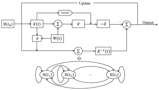
Figure 2.
Logical block diagram of the AFRNN model.
Remark 2.
The decision to utilize an RNN-based learning approach in preference to a deep learning approach was based on three key considerations. Firstly, methods such as Convolutional Neural Networks (CNNs) or Visual Transformers (ViTs) necessitate the availability of a substantial quantity of data for training purposes. However, our detection scheme is a learning-free and model-driven approach that avoids the need for redundant training. This makes the DTMF with an AFRNN model detection scheme an economically viable and adaptable option for software or hardware implementation. Secondly, deep learning approaches necessitate the mapping of unknown features from input to output. In contrast, our detection scheme is based on rigorous mathematical derivation and modeling, which renders it highly interpretable. Furthermore, it provides a systematic theoretical analysis and results to ensure its derivation. Thirdly, the DTMF method implemented in the AFRNN model can be employed to solve the Internet optimization problem in real time, thereby achieving the detection operation. Nevertheless, in analogous circumstances, the efficacy of deep learning-based methodologies can be significantly impaired.
3.1. Complexity Analysis
Here, we present a complexity analysis of floating point operations. Before discussing the time and space complexity of the AFRNN model (15), the size of the matrices and vectors involved in the algorithm needs to be clarifed some. We have and , where . Then, some flops on matrix-vector calculus [49] and storage requirements for matrix operations are introduced as follows:
- (1)
- The addition or subtraction of two vectors requires n flops.
- (2)
- Multiplication of a scalar and a vector requires n flops.
- (3)
- Multiplication of a vector and a full-rank matrix requires flops.
- (4)
- The inverse of matrix requires flops.
- (5)
- Multiplication of a scalar and a vector occupies n storage space.
- (6)
- Multiplication of a vector and a full-rank matrix occupies storage space.
- (7)
- The transpose of matrix occupies storage space.
- (8)
- The inverse of matrix occupies storage space.
In light of the above representations, calculating needs flops and occupies storage space, and calculating needs flops and occupies storage space. Thus, it costs flops for AFRNN model (15) at every time instant totally with an overall storage requisition of . Furthermore, in the field of computer science, the term “time complexity” is employed to describe the computational resources required to execute an algorithm. In contrast, “space complexity” refers to the memory space requisition during an algorithm’s execution. It is a quantitative assessment of the amount of memory an algorithm uses when processing data. Essentially, this means that an algorithm with greater computational complexity will incur a higher time complexity and space complexity. Following this premise, the computational time complexity and space complexity of the proposed AFRNN model (15) are and , respectively. For medium-sized problems, i.e., where the computational requirements grow polynomially with the problem size, the complexity of the AFRNN model (15) is acceptable in many practical applications, especially as modern computers can quickly handle large matrix operations. Matrix operations are naturally parallel, which means that the AFRNN model (15) can make good use of multi-core processors, GPUs, or distributed computing systems to further reduce computation time. Furthermore, an analytical assessment of the space complexity associated with the AFRNN model (15) underscores its pronounced superiority in computational resource management. In particular, the AFRNN model (15) shows robust adaptability to medium-scale challenges, with space requirements in the order of , congruent with the storage capacities of prevailing computing infrastructures, and it shows excellent space efficiency and memory management capabilities, which is of great significance for improving calculation efficiency and processing speed. This feature makes the AFRNN model (15) suitable not only for prototypical theoretical investigations but also for concrete engineering and scientific computational tasks.
3.2. Convergence Analysis
In order to explain the introduction of , the convergence of the model needs to be prioritized.
Theorem 2.
When solving a dynamic quadratic programming problem, the global index of the norm of the model’s allowed error converges to 0, which is:
where α represents a constant, and .
Proof.
Model (13) can be equivalent to:
Next, we can obtain:
Solving differential Equation (18), we can obtain:
Due to , we can prove as follows:
Using a known and , we can obtain the following equation:
Thus, model (13) is able to solve the dynamic quadratic programming problem in such a way that the global exponent of the steady-state error converges to 0. The proof is complete. □
Nonetheless, model (13) still suffers from a significant drawback: the convergence time of the model is almost infinitely long. In practical applications, a short time is usually needed to obtain the trajectory of the theoretical solution. Therefore, is designed to address this shortcoming.
To ensure that the Nonlinear Response Power-Law Modulation Function does not affect the convergence of the AFRNN model, we propose the following theory:
Theorem 3.
Any monotonically increasing odd function can be used as a Power-Law Modulation Function for the model without affecting its convergence.
Proof.
Lyapunov candidate function for the i-th subsystem of the AFRNN model (15) is considered as follows:
Its time derivative is:
Obviously, since the Nonlinear Response Power-Law Modulation Function is a monotonically increasing odd function, we derive the following conclusion:
In turn, we can obtain:
Therefore, the introduction of the Nonlinear Response Power-Law Modulation Function does not affect the convergence of the model and any monotonically increasing function can be used to activate AFRNN model (15). The proof is complete. □
After power-law modulation of the AFRNN model (15), the time derivative of the error function is changed. After rigorous theoretical analysis, the AFRNN model (15) under power-law modulation has an upper bound on the convergence time, and this upper bound can be adjusted by parameters. In order to verify the accelerated convergence effect of the AFRNN model (15), we propose the following theorem.
Theorem 4.
AFRNN model (15) for solving dynamic quadratic programming problems allows to converge globally in a finite time. The convergence time is capped at:
where denotes the element of the initial error vector with the largest absolute value.
Proof.
Since each element shares the same dynamic system, the subsystems of the AFRNN model (15) belonging to can be expressed as:
where is the time-varying eigenvalue of .
In the same dynamical system, must be the last to converge to 0. In other words, the time required for to converge to 0 is the maximum convergence time. Since the AFRNN model is symmetric, to simplify the proof process, we assume . Then, we can obtain:
Equation (20) can be rewritten as:
We denote ; then, we can obtain:
According to the formulae for solving first-order differential equations, we have:
According to Theorem 2, when , :
In addition, we can derive:
Based on the above derivation, an upper bound on the convergence time is obtained:
The proof is complete. □
3.3. Robustness Analysis
In engineering calculations, while the pursuit of a disturbance-free computational environment is an ideal goal, it is often unattainable due to physical constraints and practical conditions. Hence, the robustness of the model—the ability to maintain the accuracy of computation results despite the presence of higher-order residuals, hardware-induced rounding errors, and other forms of disturbances—becomes crucial. These perturbations can originate from multiple sources, including external noise caused by hardware and the working environment, as well as internal errors during data storage and signal transmission, which can be either static or dynamic.
The presence of such noise and errors clearly affects the solution algorithms. They not only reduce the performance of the algorithm but may also lead to meaningless results in practical applications. Therefore, when designing solution algorithms and computational models, it is imperative to consider these factors to ensure that the model can operate not only in an ideal state but more importantly, maintain its performance and accuracy under the complex conditions of the real world.
Firstly, we consider the impact of a type of static noise on the model, which can be described as follows:
Theorem 5.
AFRNN model can converge to a fixed range under the influence of constant noise :
Proof.
The AFRNN model (15) under constant noise can be rewritten as:
Similarly, its sub-model can be expressed as:
Define a new Lyapunov positive definite function: . This can be derived and simplified to yield the following expression:
According to the Liapunov stability principle, the results in the following three cases need to be considered separately:
(1)
If , i.e., , then is globally convergent, and we have:
When , AFRNN model Equations (4)–(7) can achieve global convergence. In this scenario, we can demonstrate that . If is within the permissible error range and , it implies that . The boundary of the steady-state error, , can diminish to 0 over time. To summarize, fluctuates within the bounded range .
(2)
At this point, and . This moment indicates that the value of depends on the sign of . Obviously, this is only a transient state, and subsequently, the state changes to case 1 and case 3.
(3)
If , then . According to the Lyapunov stability principle, gradually converges to state that satisfies .
When , similar to case 1, becomes divergent after converging to the critical point . At this moment, there are . Clearly, will diverge to the boundaries then stabilise around .
Taking the above analyses together, each subsystem of the AFRNN model eventually reaches stability at and necessarily satisfies b. Therefore, we can conclude the following:
At this point, the proof is complete. □
The input to the noise is typically not constant; therefore, expanding our assumptions regarding the noise structure becomes necessary:
AFRNN model analyses the impact of periodic and non-periodic bounded noise, even when information on the derivatives of the noise is unavailable. This theorem is presented:
Theorem 6.
Under conditions of bounded time-varying noise , the steady-state error of the AFRNN model converges to a specific range with high confidence. It is important to acknowledge, however, that this model may not be suitable for all scenarios and further research may be necessary to fully understand its limitations:
Proof.
While the AFRNN model primarily utilizes a tonal power law structure, it is worth noting that linear functions can also be considered as a subset of this structure. For the purposes of simplifying the analysis process, we have defined this subset as a linear function. As a result, can be further simplified as follows:
The submodel that corresponds to this is expressed as:
By combining Equation (31) with the general solution of the first-order differential equation, the following expression is obtained:
The equation can be simplified to:
In which . Knowing , we have:
The following inequality can be derived from the trigonometric inequality:
The following inequality is derived based on Lobida’s law:
It can be inferred from Equation (32) that:
At this point, the proof is complete. □
4. Identification Experiments and Accuracy Assessment
This section introduces data sources and preprocessing. For comparison, we selected classic remote sensing target extraction methods such as ACE, CEM, and MF for comparison to verify our high accuracy and stability. It should be noted that all experiments are conducted using MATLAB 2017A on a computer with Windows 10, an AMD Ryzen 5 3600 6-Core CPU @3.60 GHz, and 16 GB RAM. The experimental parameters are as follows: dynamic penalty factor , scale factor and nonlinear scale .
4.1. Dataset
This research investigates the Zhanjiang Port Fishery Port region and Tongming Port in Zhanjiang City, as depicted in the red boxes in in Figure 3, serving as the primary research areas. On-site aerial photography was conducted in these regions to systematically collect data for experimentation. Image source for Figure 3 is from earthexplorer.
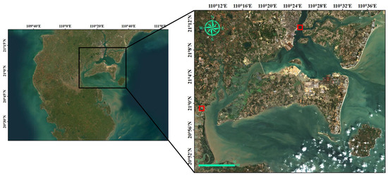
Figure 3.
Research region.
Furthermore, the remote sensing images presented in this paper were captured using the DJI M300 RTK (Shenzen, China), which is developed and manufactured by DJI in Shenzhen, China. The DJI M300 RTK is equipped with a high-precision RTK navigation system, which is capable of achieving centimeter-level positioning accuracy. This ensures that the vehicle is able to fly stably in the air and to accurately reach the designated destination. The UAV in this study is equipped with the MS600 PRO (Tianjin, China) multispectral camera, which is a custom-developed multispectral camera based on the DJI PSDK, manufactured by YUSENSE in Qingdao, China. It can be seamlessly connected to the DJI M200 and M300 RTK UAV flight platforms. The MS600 PRO has six spectral channels, each of which employs a 1.2-megapixel high-dynamic-range full-range shutter, a CMOS detector, six waveforms, and a 1.2-megapixel high-dynamic-range full-range shutter, and a CMOS detector. The CMOS detector has six bands. The acquisition of UAV image data is influenced by a number of factors, including flight speed, flight altitude, weather conditions, attitude orientation, and the parameter settings of the gimbaled intelligent camera. These factors have the potential to significantly impact the quality and effectiveness of the acquired data. In order to ensure the acquisition of high-quality image data, a significant number of preliminary tests must be conducted in order to determine the optimal settings. In this paper, the acquisition was conducted under clear and cloudless weather conditions. It is recommended that the flight altitude be set at 100 and 150 meters. The objective of these measures is to optimize the image acquisition process and ensure the quality of the image data.
During UAV aerial photography, remote sensing images may be affected by a variety of factors, including optical distortion and other issues. To overcome these problems, an image processing pipeline is crucial, which includes steps such as image stitching and orthorectification. Before orthorectification, the original data need to be initially processed, which includes counting target key points, automatic aerial triangulation, bundle block adjustment, and camera self-calibration, etc., to remove factors that affect image quality, such as UAV calibration gray plate, underexposure or overexposure, and inaccurate focus. This research uses Pix4Dmapper automated 3D modeling software and ENVI to preprocess UAV remote sensing data.
4.2. Parameter Descriptions
Confusion matrices [50] play a crucial role in remote sensing image extraction, providing a basic and intuitive method for evaluating the accuracy of extraction models. It quantifies model performance by comparing the model’s prediction results on test images with real ground object images and counting the number of correct and incorrect observations. The confusion matrix is particularly useful when dealing with binary classification problems because it provides a clear analytical framework for the positive (1, Positive) or negative (0, Negative) results predicted by the model. The core components of the confusion matrix include four basic parameters: true examples (TP), true negatives (TN), false positives (FP) and false negatives (FN). These parameters describe in detail the various possibilities of model predictions. The results are shown in Table 1. These key parameters are the cornerstone of understanding and evaluating the performance of a classification model. They not only help us intuitively see the performance of the model in actual tests but are also important indicators for calculating model efficiency, such as accuracy, recall, precision and F1 scores, etc.

Table 1.
Region 1 extraction accuracy evaluation results.
The confusion matrix is an extremely valuable tool in remote sensing image classification tasks, but its limitations when dealing with large-scale data sets cannot be ignored. The assessment of the quality of a model based on the mere counting of pixels in remote sensing images may prove to be inadequate. This is particularly pertinent in the field of remote sensing, where the quantity of data is voluminous and the intricacy of the subject matter is considerable. Therefore, in order to achieve a more comprehensive model performance evaluation, the basic statistical results of the confusion matrix must be used in conjunction with other detailed evaluation indicators, including overall accuracy (OA), precision, recall, F-score, and calculating time (CT). The formulae for these are as follows:
Furthermore, this research employs the KAPPA coefficient [51] as the principal indicator for the evaluation of model performance. The formula is as follows:
4.3. Extraction Results and Accuracy Evaluation
In this subsection, we divide the experiments into three different sub-subsections, with the first two focusing on different UAV imaging altitudes: 100 m and 150 m. This division corresponds to the different flight altitudes used during the experiments. To evaluate the generalization ability of our proposed method and verify its performance, we use the public HRSC2016 [52] dataset in Section 4.3.3. This dataset is known for its diversity and complexity, making it an excellent benchmark for testing our method. In addition, we present a structured evaluation framework in Section 4.2 to facilitate a detailed comparison between the DTMF method and three other classic ship extraction methods. This framework aims to comprehensively evaluate their performance under different imaging conditions, especially in terms of ship extraction accuracy.
4.3.1. Imaging Height 100 m
This sub-subsection presents the results of an experimental investigation conducted on images captured at a flight height of 100 m. The numerical results of different precisions recorded in Table 1 further quantify the effectiveness of these four methods in extracting ships in different regions, providing a detailed performance comparison. Using the visual extraction results displayed in Figure 4, we show the extraction effects of the four methods in an intuitive way, so that the evaluation process is not limited to numerical analysis, but also provides a visual comparison.
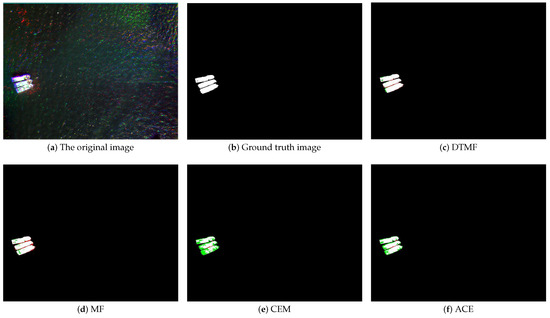
Figure 4.
Results of different methods for ship extraction in sample region 1 of UAV remote sensing image.
This research uses the graythresh function in MATLAB, which automatically selects the optimal threshold based on the OTSU algorithm to convert the image into a binary image. Through threshold segmentation, we obtain clear extraction results in the form of binary images. It is worth noting that, in order to ensure the fairness of the research and avoid biases that may be introduced by customized pre-processing and post-processing processes for remote sensing images, the image processing processes and related parameter settings of all methods are consistent with the methods used in this research. This step ensures the objectivity and comparability of the analysis results and provides a reliable basis for evaluating the performance of different algorithms in ground object detection.
After threshold segmentation, it is necessary to visually compare the extraction map of each algorithm with the true value map of the feature to be extracted Figure 4b and evaluate the parameters through index calculation. It can be intuitively seen from Figure 4c–f that the method in this research has the best fresh extraction effect.
In addition, we represent different categories in the contrast map by using four colors, where red is used to mark misclassified ship regions, green represents missed extraction regions, and black and gray represent seawater and land, respectively. This method not only enhances the interpretability of results but also facilitates the identification of errors and omissions at a glance.
As can be seen from Figure 4a, there are significant red, green, and blue (RGB) noise spots in the image, which may be caused by sensor abnormalities during image capture or the special properties of spectral reflection. There is widespread noise in the image, which may be misidentified as a small ship or part of a ship. We can intuitively see that the dtmf method can accurately extract the shape and outline of the ship, while the other three methods all have a certain degree of missed detection and value detection of the shape.
From Table 1, we can see that the DTMF method shows excellent performance on almost all evaluation metrics, especially in terms of overall precision (0.9988) and recall (0.9668), which shows that it is very good at correctly identifying ship pixels efficient. In addition, DTMF also exhibits a high Kappa coefficient (0.9768), indicating that its results are highly consistent and reliable. Although the precision rate of DTMF (0.9201) is slightly lower than that of CEM (0.9719), the recall rate of CEM is significantly lower (0.5836), indicating that although it can accurately identify ships, it misses a large number of actual ship targets. This low recall may limit its utility in practical applications.
Figure 5a shows several ships in relatively dark water. The ships are arranged in a rough diagonal shape, pointing from the upper left to the lower right. The largest ship is at the bottom of the array, with two smaller ships above it. While the ships themselves are more visible, there is still a lot of colored noise in the background. These noises visually resemble small boats or other objects, which can pose a challenge to pixel-based detection algorithms. Color distortion in the image creates a large amount of red and green noise, and this color distribution may affect the performance of the extraction method.
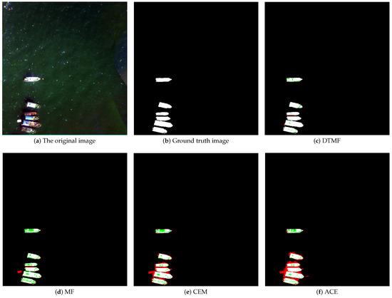
Figure 5.
Results of different methods for ship extraction in sample region 2 of UAV remote sensing image.
As can be seen from Figure 5c–f, the dtmf method can effectively overcome the interference of background noise and extract the shape and contour of the hull. The other three methods all experienced a certain degree of missed detections and false detections.
We can conclude from Table 2 that the DTMF method performs optimally in sample region 2. It achieved an OA of 0.9979, meaning it was able to correctly distinguish between ship and non-ship pixels in most cases. DTMF also performed best in terms of precision, reaching 0.9385, indicating that its recognition results for ships have a high proportion of true examples. In terms of Recall, DTMF leads with a result of 0.9582 and can identify most of the real ship pixels. At the same time, its AA and Kappa coefficient are 0.9784 and 0.9471, respectively, both showing high classification consistency and reliability.
Table 2.
Region 2 extraction accuracy evaluation results.
Figure 6a depicts sample region 3, wherein the ship is moored alongside the pier. Due to the phenomenon of light reflection, the spectral characteristics of the ship are very similar to those of the pier. This results in the phenomenon of different objects having the same spectrum. Figure 6c–f illustrates the extraction effects of various methods. It can be observed that the DTMF method demonstrates the most effective background suppression, while also retaining the outline of the ship to the greatest extent. Table 3 shows that the DTMF method performs best in terms of OA (0.9989), Recall (0.9236), AA (0.9617), and KAPPA coefficient (0.9528). At the same time, the FA of the DTMF method is extremely low (0.0002) and the CT is the shortest (0.0141), indicating that it not only has an advantage in accuracy but also has high computational efficiency. Various indicators show that the DTMF method can accurately and efficiently extract ships while dealing with the complexity of the background and the similarity of spectral features in sample region 3, showing the best overall performance.
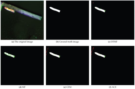
Figure 6.
Results of different methods for ship extraction in sample region 3 of UAV remote sensing image.
Table 3.
Region 3 extraction accuracy evaluation results.
4.3.2. Imaging Height 150 m
In this sub-subsection, an experimental investigation is conducted on images captured at an altitude of 150 m.
Figure 7a presents a remote sensing image of a group of ships at night or under low light conditions. The ships are distributed throughout the image, and their orientations and positions vary, with some aligned in a straight line and others slightly off. There is also a large amount of color noise in the image, which may be due to noise generated by the light-sensitive elements of the remote sensing equipment under low-light conditions. As can be seen in Figure 7c–f, DTMF method can detect the edges and contours of the ship very well. While the other three methods have misdetected the edges. As illustrated in Figure 7c–f, the DTMF method is capable of accurately detecting the edges and contours of the ship. In contrast, the other three methods have incorrectly identified the edges. The clarity of ship edges is a crucial factor in the detection of remote sensing targets, as it enables the algorithms to correctly segment and identify these targets. Table 4 indicates that the DTMF method once again demonstrates its superiority in the extraction of ships from remote sensing images, as evidenced by the results of the performance evaluation of sample region 3. All the metrics have been optimized.
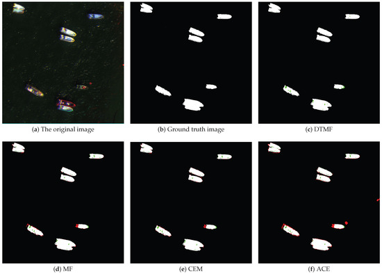
Figure 7.
Results of different methods for ship extraction in sample region 4 of UAV remote sensing image.
Table 4.
Region 4 extraction accuracy evaluation results.
As illustrated in Figure 8a, sample region 5 exhibits a luxuriant growth of trees, which exudes a verdant hue. The low color contrast between the boat color and the surrounding seawater and forest may present a challenge for the threshold-based segmentation method. Additionally, the reflected light from the water surface may influence the pixel values in the image, thereby increasing the difficulty in distinguishing the boat from the reflective water surface. As illustrated in Figure 8c–f, the DTMF method is the most effective of the four in terms of extraction results, with no instances of misdetection of the ship contours. However, the DTMF method does exhibit misdetection of the ship contours. The remaining three methods mis-extract the shoals and water bodies as ship hulls.
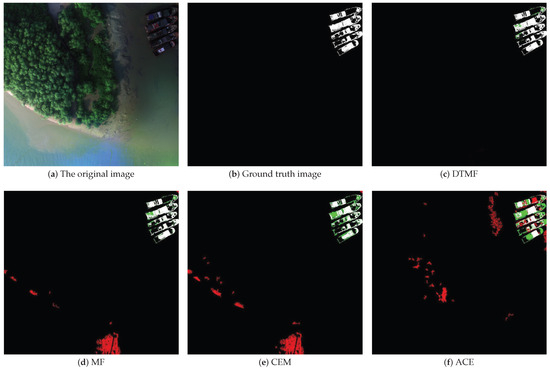
Figure 8.
Results of different methods for ship extraction in sample region 5 of UAV remote sensing image.
As illustrated in Table 5, the performance metrics for each method in the performance evaluation in sample region 5 demonstrate that the DTMF method is significantly more effective than the other three methods. The DTMF method has an OA of 0.9964, indicating that it is capable of accurately distinguishing between ship and non-ship pixels in the majority of cases. Furthermore, the DTMF method exhibits the highest precision at 0.8733. Although this value is lower than that of the DTMF method in sample regions 1–3 for DTMF method, it implies that DTMF has relatively few false positives when the predicted pixel is a ship in sample region 4. As demonstrated by the recall, the DTMF method is able to correctly identify true ship pixels at a rate of 0.9450. This metric is of significant importance, as it demonstrates the efficacy of the DTMF method in accurately identifying genuine ship pixels. The Kappa coefficient of DTMF reaches 0.9059, which is considerably higher than those of other methods. In contrast, MF, CEM and ACE all exhibit lower performance, particularly in terms of precision and Kappa coefficient.
Table 5.
Region 5 extraction accuracy evaluation results.
Figure 9a depicts sample region 6, which exhibits a more complex background that may impede the ship extraction process to some extent. The ships were situated in close proximity to the jetty, and the boundaries between them were not entirely clear. Additionally, the complex rust and mottled colors on the hulls of ships can create challenges in spectral differentiation. The containers or cargo on the quayside may also be spectrally similar to ships, further complicating the extraction process. The hulls of different ships also exhibit different spectral characteristics. The simultaneous existence of spectra that are different for the same object and objects that are different for the same spectrum makes the extraction task more challenging. In Figure 9c–f, the results of the different detection methods are presented. The DTMF method is capable of overcoming the issue of homogeneous and heterogeneous spectra by suppressing the same interfering background as the hull spectra. Furthermore, all the hulls with different spectra are extracted. The DTMF method is the closest to the real situation on the ground, while the other methods show multiple missed or false detections, with the CEM and ACE methods in particular having a high number of false alarms.
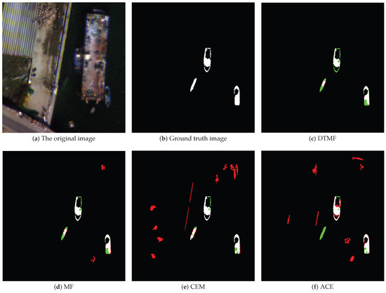
Figure 9.
Results of different methods for ship extraction in sample region 6 of UAV remote sensing image.
As demonstrated in Table 6, the DTMF method exhibited the most optimal performance in the assessment of ship extraction within the sample region 6. In particular, the DTMF method achieved a value of 0.9946 in terms of OA, which highlights its accuracy in the ship extraction task. Although the MF method exhibits a slightly superior precision of 0.8482, indicating enhanced accuracy in ship classification, the DTMF method also demonstrates a high level of precision (0.8048). In terms of recall, the CEM method leads with 0.8359, demonstrating a superior ability to recognize genuine ship pixels. However, DTMF maintains a commendable level of recognition with a recall of 0.7017. In the evaluation of AA, the CEM method stands out with 0.9128, demonstrating its balanced detection ability across all categories. Meanwhile, the DTMF method also achieves an AA of 0.8699, which ensures its consistent performance in the detection of different types of ships. Most importantly, DTMF outperforms other methods with a Kappa coefficient of 0.8268, demonstrating its advantage in classification consistency. While other methods may have a slight advantage in specific metrics, the overall performance of DTMF is significantly superior in terms of accuracy, reliability, and consistency.
Table 6.
Region 6 extraction accuracy evaluation results.
4.3.3. HRSC2016
This sub-subsection employs the public dataset HRSC2016 to assess the generalization capacity of the proposed method. Four distinct scenes from the HRSC2016 dataset were selected to assess the extraction capabilities of the various methods. The results of the visualization, as shown in Figure 10, demonstrate that the proposed method is able to extract the target contour with the greatest accuracy, while also avoiding erroneous extraction in the four groups of experiments. The quantitative results are presented in Table 7.
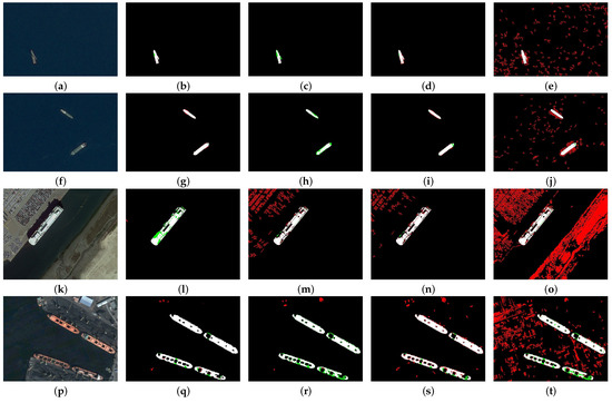
Figure 10.
The results of the visualization of the extraction effects of different methods were verified in four different scenarios. (a–e) represent the extraction experiments of test 1. The images are presented from left to right, with the original image at the top, followed by the DTMF extraction results, MF extraction results, CEM extraction results, and ACE extraction results. (f–j) represent the extraction experiments of test 2, with the original image displayed from left to right. The subsequent images are the DTMF extraction results, MF extraction results, CEM extraction results, and ACE extraction results. (k–o) represent the extraction experiments of test 3, with the original image displayed from left to right. The subsequent images are the DTMF extraction results, MF extraction results, CEM extraction results, and ACE extraction results. (p–t) represent the extraction experiments of test 4, with the original image displayed on the left and the DTMF, MF, CEM and ACE extraction results displayed in succession.
Table 7.
HRSC2016 extraction experiment quantitative results.
As demonstrated in Table 7, the quantitative results reveal that the four methods of DTMF, MF, CEM and ACE exhibit varying degrees of efficacy in the four tests of HRSC2016. The DTMF method demonstrated the most optimal performance in OA, F-score, KAPPA coefficient and computational efficiency, exhibiting exceptional capabilities in terms of high precision, high recall and rapid processing. The overall accuracy of the method exceeds 0.99 in all four tests, and its recall rate and F-score demonstrate its resilience in complex backgrounds, rendering it an optimal choice for real-time applications. Although the MF method achieves extremely high accuracy, especially up to 0.9997 in some tests, its recall rate is relatively low, indicating that it has certain deficiencies in detecting all targets. Concurrently, the MF method has the shortest calculation time and is therefore well-suited to application scenarios that are sensitive to calculation time. The CEM method demonstrates excellent recall performance, with a recall rate of nearly 1 in most tests. This evidence supports the assertion that the method is highly effective in object detection. Nevertheless, the accuracy and overall performance of the method are subject to fluctuations, and its computational efficiency is moderate. Although the ACE method exhibits a high recall rate, its low precision and lengthy calculation process restrict its practical applicability. The overall precision and comprehensive score of the ACE method are the lowest among the four methods. In conclusion, the DTMF method demonstrates satisfactory performance across a range of indicators, thereby corroborating its capacity for generalization across disparate data sets.
4.4. Discussion
The efficacy of the DTMF method is demonstrated in a series of experimental analyses across a range of scenarios. The DTMF method is effective in processing remote sensing images containing multiple targets and complex background interference. It is particularly noteworthy for its ability to enhance target signals, dynamically adapt to changing conditions, reduce background interference, optimize resources, and ensure system robustness. In the extraction of targets from UAV remote sensing images captured at varying altitudes, the DTMF method demonstrated superior performance, as evidenced by the OA reaching 0.99 and the Kappa coefficient reaching 0.82, both of which were higher than those of the three comparison methods. Although MF and CEM may occasionally be comparable to DTMF in some indicators, DTMF consistently demonstrates superior performance in almost all indicators and sample areas. Furthermore, it effectively suppresses the phenomenon of different objects with the same spectrum and different spectra with the same object in the remote sensing target extraction task, and verifies the stability of DTMF in ship detection in different scenarios. In the experimental extraction task of HRSC2016, the OA of the DTMF method reached 0.99, while the KAPPA coefficient reached 0.86, both of which were higher than those of the three comparison methods. It is necessary to verify the ability of the DTMF method to generalize across different datasets.
5. Conclusions
This research presents a DTMF method for the extraction of ships from UAV remote sensing images. In contrast to the MF, DTMF is capable of adapting to the dynamic changes in the system, ensuring that the system is able to accurately track the target spectral vectors over time and provide sustained detection performance at different time points. Furthermore, in order to address DTMF, this paper develops the AFRNN model from the perspective of the control domain. ARFNN model introduces an adaptive feedback term based on the gradient RNN and designs a special nonlinear projection function, which can be dynamically adapted according to the changes in the input data or the environment. This eliminates the time lag problem. Subsequently, this paper presents rigorous theoretical proof that the AFRNN model for solving DTMF has high extraction accuracy and strong robustness, thereby ensuring the extraction performance of DTMF in complex environments. Finally, the quantitative and visual results demonstrate that the DTMF method exhibits clear advantages over other classical remote sensing target extraction methods in addressing the challenges of ’same object, different spectra’ and ’same spectrum, different objects’ in complex scenes. In the extraction experiment, this method with an overall accuracy (OA) of over 0.99 and a Kappa coefficient exceeding 0.82. This demonstrates that the method has a significant advantage in effectively overcoming the phenomenon of missed detection and false detection. The extraction effect is clear, the accuracy rate is high, and the leakage and misdetection can be effectively overcome. This evidence demonstrates the efficacy and superiority of the DTMF method as a means of extracting ships from UAV remote sensing images.
Author Contributions
Conceptualization, S.D. and D.F.; methodology, S.D. and Y.S.; software, S.D., Y.S. and Y.L.; validation, D.F.; formal analysis, S.D. and Y.S.; investigation, D.F.; resources, S.D.; data curation, S.D. and Y.Z.; writing—original draft preparation, S.D. and D.F.; writing—review andediting, S.D. and Y.S.; visualization, S.D. and Y.L.; supervision, S.D. and D.F.; project administration, D.F.; funding acquisition, D.F. All authors have read and agreed to the publishedversion of the manuscript.
Funding
This research was funded in part by the National Key Research and Development Program of China under Grant 2022yFC3103101, Key Special Project for Introduced Talents Team of Southern Marine Science and Engineering Guangdong Laboratory under Contract GML2021GD0809, National Natural Science Foundation of China under Contract 42206187, Key projects of the Guangdong Education Department under Grant 2023ZDZX4009.
Data Availability Statement
Data are contained within the article.
Conflicts of Interest
The authors declare no conflicts of interest.
References
- Liu, J.; Wen, G. Maritime Target Detection and Tracking. In Proceedings of the 2019 IEEE 2nd International Conference on Automation, Electronics and Electrical Engineering (AUTEEE), Shenyang, China, 22–24 November 2019; IEEE: Piscataway, NJ, USA, 2019; pp. 309–314. [Google Scholar]
- Perera, L.P.; Oliveira, P.; Soares, C.G. Maritime Traffic Monitoring Based on Vessel Detection, Tracking, State Estimation, and Trajectory Prediction. IEEE Trans. Intell. Transp. Syst. 2012, 13, 1188–1200. [Google Scholar] [CrossRef]
- Knapp, S.; Franses, P.H. Comprehensive Review of the Maritime Safety Regimes: Present Status and Recommendations for Improvements. Transp. Rev. 2010, 30, 241–270. [Google Scholar] [CrossRef]
- Peters, K. Deep Routeing and the Making of ‘Maritime Motorways’: Beyond Surficial Geographies of Connection for Governing Global Shipping. Geopolitics 2020, 25, 43–64. [Google Scholar] [CrossRef]
- Pedersen, P.T. Review and Application of Ship Collision and Grounding Analysis Procedures. Mar. Struct. 2010, 23, 241–262. [Google Scholar] [CrossRef]
- Chaturvedi, S.K.; Sekhar, R.; Banerjee, S.; Kamal, H. Comparative Review Study of Military and Civilian Unmanned Aerial Vehicles (UAVs). INCAS Bull. 2019, 11, 181–182. [Google Scholar] [CrossRef]
- Mohd Noor, N.; Abdullah, A.; Hashim, M. Remote Sensing UAV/UAV and Its Applications for Urban Areas: A Review. In IOP Conference Series: Earth and Environmental Science; IOP Publishing: Bristol, UK, 2018; Volume 169. [Google Scholar]
- Yao, H.; Qin, R.; Chen, X. Unmanned Aerial Vehicle for Remote Sensing Applications—A Review. Remote Sens. 2019, 11, 1443. [Google Scholar] [CrossRef]
- Shakhatreh, H.; Sawalmeh, A.; Al-Fuqaha, A.; Dou, Z.; Almaitta, E.; Khalil, I.; Othman, N.S.; Khreishah, A.; Guizani, M. Unmanned Aerial Vehicles (UAVs): A Survey on Civil Applications and Key Research Challenges. IEEE Access 2019, 7, 48572–48634. [Google Scholar] [CrossRef]
- Tilon, S.; Nex, F.; Vosselman, G.; Sevilla de la Llave, I.; Kerle, N. Towards improved unmanned aerial vehicle edge intelligence: A road infrastructure monitoring case study. Remote Sens. 2022, 14, 4008. [Google Scholar] [CrossRef]
- Turan, M.; Ferhat, G.; Adil, A. An Analytical Approach to the Concept of Counter-UA Operations (CUAOPS) SWOT Analysis of Unmanned Aircraft Systems. J. Intell. Robot. Syst. 2012, 65, 73–91. [Google Scholar] [CrossRef]
- Fraga-Lamas, P.; Fernández-Caramés, T.M. Tactical edge iot in defense and national security. In IoT for Defense and National Security; Wiley: Hoboken, NJ, USA, 2022; pp. 377–396. [Google Scholar]
- Quigley, M.; Goodrich, M.A.; Griffiths, S.; Eldredge, A.; Beard, R.W. Target Acquisition, Localization, and Surveillance Using a Fixed-Wing Mini-UAV and Gimbaled Camera. In Proceedings of the 2005 IEEE International Conference on Robotics and Automation, Barcelona, Spain, 18–22 April 2005; IEEE: Piscataway, NJ, USA, 2005. [Google Scholar]
- Kerekes, J.P.; Baum, J.E. Spectral Imaging System Analytical Model for Subpixel Object Detection. IEEE Trans. Geosci. Remote Sens. 2002, 40, 1088–1101. [Google Scholar] [CrossRef]
- Manolakis, D.; Siracusa, C.; Shaw, G. Hyperspectral Subpixel Target Detection Using the Linear Mixing Model. IEEE Trans. Geosci. Remote Sens. 2001, 39, 1392–1409. [Google Scholar] [CrossRef]
- Turin, G. An Introduction to Matched Filters. IRE Trans. Inf. Theory 1960, 6, 311–329. [Google Scholar] [CrossRef]
- Chaudhuri, S.; Chatterjee, S.; Katz, N.; Nelson, M.; Goldbaum, M. Detection of Blood Vessels in Retinal Images Using Two-Dimensional Matched Filters. IEEE Trans. Med Imaging 1989, 8, 263–269. [Google Scholar] [CrossRef] [PubMed]
- Manolakis, D.; Marden, D.; Shaw, G.A. Hyperspectral Image Processing for Automatic Target Detection Applications. Linc. Lab. J. 2003, 14, 79–116. [Google Scholar]
- Stefanou, M.S.; Kerekes, J.P. Image-Derived Prediction of Spectral Image Utility for Target Detection Applications. IEEE Trans. Geosci. Remote Sens. 2009, 48, 1827–1833. [Google Scholar] [CrossRef]
- Farrand, W.H.; Harsanyi, J.C. Mapping the Distribution of Mine Tailings in the Coeur d’Alene River Valley, Idaho, through the Use of a Constrained Energy Minimization Technique. Remote Sens. Environ. 1997, 59, 64–76. [Google Scholar] [CrossRef]
- Ren, H.; Chang, C.-I.; Du, Q.; Jensen, J.R. Comparison between Constrained Energy Minimization-Based Approaches for Hyperspectral Imagery. In Proceedings of the IEEE Workshop on Advances in Techniques for Analysis of Remotely Sensed Data, Greenbelt, MD, USA, 27–28 October 2003; IEEE: Piscataway, NJ, USA, 2003. [Google Scholar]
- Bidon, S.; Besson, O.; Tourneret, J.-Y. The Adaptive Coherence Estimator is the Generalized Likelihood Ratio Test for a Class of Heterogeneous Environments. IEEE Signal Process. Lett. 2008, 15, 281–284. [Google Scholar] [CrossRef]
- Yang, S.; Shi, Z.; Tang, W. Robust Hyperspectral Image Target Detection Using an Inequality Constraint. IEEE Trans. Geosci. Remote Sens. 2014, 53, 3389–3404. [Google Scholar] [CrossRef]
- Xiong, Y.; Wang, J.; Zhang, S.; Zhang, Y. Ice Identification with Error-Accumulation Enhanced Neural Dynamics in Optical Remote Sensing Images. Remote Sens. 2023, 15, 5555. [Google Scholar] [CrossRef]
- Yang, S.; Shi, Z. SparseCEM and SparseACE for Hyperspectral Image Target Detection. IEEE Geosci. Remote Sens. Lett. 2014, 11, 2135–2139. [Google Scholar] [CrossRef]
- Chen, Y.; Fu, D.; Wang, D.; Huang, H.; Si, Y.; Du, S. Noise-Tolerant Matched Filter Scheme Supplemented with Neural Dynamics Algorithm for Sea Island Extraction. CAAI Trans. Intell. Technol. 2024, 1, 12323. [Google Scholar] [CrossRef]
- Chaillan, F.; Courmontagne, P. On the Use of the Stochastic Matched Filter for Ship Wake Detection in SAR Images. In Proceedings of the OCEANS 2006 Conference, Boston, MA, USA, 18–21 September 2006; IEEE: Piscataway, NJ, USA, 2006. [Google Scholar]
- Kim, K.; An, H.; Kim, J. Probabilistic Ship Detection and Classification Using Deep Learning. Appl. Sci. 2018, 8, 936. [Google Scholar] [CrossRef]
- Zhang, R.; Yao, J.; Zhang, K.; Feng, C.; Zhang, J. S-CNN-Based Ship Detection from High-Resolution Remote Sensing Images. Int. Arch. Photogramm. Remote Sens. Spat. Inf. Sci. 2016, 41, 423–430. [Google Scholar] [CrossRef]
- Wang, Y.; Wang, B.; Huo, L.; Fan, Y. GT-YOLO: Nearshore Infrared Ship Detection Based on Infrared Images. J. Mar. Sci. Eng. 2024, 12, 213. [Google Scholar] [CrossRef]
- Zhao, S.; Luo, Y.; Zhang, T.; Guo, W.; Zhang, Z. A Domain Specific Knowledge Extraction Transformer Method for Multisource Satellite-Borne SAR Images Ship Detection. ISPRS J. Photogramm. Remote Sens. 2023, 198, 16–29. [Google Scholar] [CrossRef]
- Najafabadi, M.M.; Villanustre, F.; Khoshgoftaar, T.M.; Seliya, N.; Wald, R.; Muharemagic, E. Deep learning applications and challenges in big data analytics. J. Big Data 2015, 2, 1. [Google Scholar] [CrossRef]
- Sun, C.; Shrivastava, A.; Singh, S.; Gupta, A. Revisiting unreasonable effectiveness of data in deep learning era. In Proceedings of the IEEE International Conference on Computer Vision, Venice, Italy, 22–29 October 2017. [Google Scholar]
- Alzubaidi, L.; Bai, J.; Al-Sabaawi, A.; Santamaría, J.; Albahri, A.S.; Al-dabbagh, B.S.N.; Fadhel, M.A.; Manoufali, M.; Zhang, J.; Al-Timemy, A.H.; et al. A survey on deep learning tools dealing with data scarcity: Definitions, challenges, solutions, tips, and applications. J. Big Data 2023, 10, 46. [Google Scholar] [CrossRef]
- Lai, Z.; Chauhan, J.; Chen, D.; Dugger, B.N.; Cheung, S.C.; Chuah, C. Semi-Path: An interactive semi-supervised learning framework for gigapixel pathology image analysis. Smart Health 2023, 32, 100474. [Google Scholar] [CrossRef]
- Zhang, K.; Yang, X.; Xu, L.; Thé, J.; Tan, Z.; Yu, H. Enhancing coal-gangue object detection using GAN-based data augmentation strategy with dual attention mechanism. Energy 2024, 287, 129654. [Google Scholar] [CrossRef]
- Dou, B.; Zhu, Z.; Merkurjev, E.; Ke, L.; Chen, L.; Jiang, J.; Zhu, Y.; Liu, J.; Zhang, B.; Wei, G.W. Machine learning methods for small data challenges in molecular science. Chem. Rev. 2023, 13, 8736–8780. [Google Scholar] [CrossRef] [PubMed]
- Rocks, J.W.; Mehta, P. Memorizing without overfitting: Bias, variance, and interpolation in overparameterized models. Phys. Rev. Res. 2022, 4, 013201. [Google Scholar] [CrossRef] [PubMed]
- Castiglioni, I.; Rundo, L.; Codari, M.; Di Leo, G.; Salvatore, C.; Interlenghi, M.; Gallivanone, F.; Cozzi, A.; D’Amico, N.C.; Sardanelli, F. AI applications to medical images: From machine learning to deep learning. Phys. Med. 2022, 83, 9–24. [Google Scholar] [CrossRef]
- Zhang, Y.; Wang, J. Recurrent Neural Networks for Nonlinear Output Regulation. Automatica 2001, 37, 1161–1173. [Google Scholar] [CrossRef]
- Shi, Y.; Li, S.; Wang, L.; Liu, Z. Novel Discrete-Time Recurrent Neural Networks Handling Discrete-Form Time-Variant Multi-Augmented Sylvester Matrix Problems and Manipulator Application. IEEE Trans. Neural Netw. Learn. Syst. 2020, 33, 587–599. [Google Scholar] [CrossRef] [PubMed]
- Zhang, Y.; Wang, J.; Shi, Y.; Li, S. A Recurrent Neural Network Approach for Visual Servoing of Manipulators. In Proceedings of the 2017 IEEE International Conference on Information and Automation (ICIA), Macao, China, 18–20 July 2017; IEEE: Piscataway, NJ, USA, 2017. [Google Scholar]
- Liao, S.; Yin, Y.; Tang, Y.; Wang, J. Modified Gradient Neural Networks for Solving the Time-Varying Sylvester Equation with Adaptive Coefficients and Elimination of Matrix Inversion. Neurocomputing 2020, 379, 1–11. [Google Scholar] [CrossRef]
- Luo, X.; Huang, J.; Yang, S.; Li, S. A Novel Recurrent Neural Network for Robot Control. In Robot Control and Calibration: Innovative Control Schemes and Calibration Algorithms; Springer Nature: Singapore, 2023; pp. 33–49. [Google Scholar]
- Xiao, L.; Zhang, Y. Different Zhang Functions Resulting in Different ZNN Models Demonstrated via Time-Varying Linear Matrix–Vector Inequalities Solving. Neurocomputing 2013, 121, 140–149. [Google Scholar] [CrossRef]
- Zhang, Y.; Chen, K.; Tan, H.-Z. Performance Analysis of Gradient Neural Network Exploited for Online Time-Varying Matrix Inversion. IEEE Trans. Autom. Control 2009, 54, 1940–1945. [Google Scholar] [CrossRef]
- Jin, L.; Lin, W.; Li, S. Gradient-Based Differential Neural-Solution to Time-Dependent Nonlinear Optimization. IEEE Trans. Autom. Control 2022, 68, 620–627. [Google Scholar] [CrossRef]
- Jarlebring, E.; Poloni, F. Iterative Methods for the Delay Lyapunov Equation with T-Sylvester Preconditioning. Appl. Numer. Math. 2019, 135, 173–185. [Google Scholar] [CrossRef]
- Hunger, R. Floating Point Operations in Matrix-Vector Calculus; Institute for Circuit Theory and Signal Processing, Munich University of Technology: Munich, Germany, 2005; Volume 2019. [Google Scholar]
- Goutte, C.; Gaussier, E. A Probabilistic Interpretation of Precision, Recall and F-Score, with Implication for Evaluation. In Proceedings of the European Conference on Information Retrieval, Santiago de Compostela, Spain, 21–23 March 2005; Springer: Berlin/Heidelberg, Germany, 2005. [Google Scholar]
- Bloch, D.A.; Kraemer, H.C. 2 × 2 Kappa Coefficients: Measures of Agreement or Association. Biometrics 1989, 45, 269–287. [Google Scholar] [CrossRef] [PubMed]
- Liu, Z.; Wang, H.; Weng, L.; Yang, Y. Ship rotated bounding box space for ship extraction from high-resolution optical satellite images with complex backgrounds. IEEE Geosci. Remote Sens. Lett. 2016, 13, 1074–1078. [Google Scholar] [CrossRef]


Disclaimer/Publisher’s Note: The statements, opinions and data contained in all publications are solely those of the individual author(s) and contributor(s) and not of MDPI and/or the editor(s). MDPI and/or the editor(s) disclaim responsibility for any injury to people or property resulting from any ideas, methods, instructions or products referred to in the content. |
© 2024 by the authors. Licensee MDPI, Basel, Switzerland. This article is an open access article distributed under the terms and conditions of the Creative Commons Attribution (CC BY) license (https://creativecommons.org/licenses/by/4.0/).