Abstract
Unlike uniform linear arrays (ULAs), coprime arrays require fewer physical sensors yet provide higher degrees of freedom (DOF) and larger array apertures. However, due to the existence of “holes” in the differential co-array, the target detection performance deteriorates, especially in adaptive beamforming. To address these challenges, this paper proposes an efficient and robust adaptive beamforming algorithm leveraging coprime array interpolation. The algorithm eliminates unwanted signals and uses the Gauss–Legendre quadrature method to reconstruct an Interference-plus-Noise Covariance Matrix (INCM), thereby obtaining the beamforming coefficients. Unlike previous techniques, we utilize a virtual interpolated ULA to expand the aperture, enabling the acquisition of a high-dimensional covariance matrix. Additionally, a projection matrix is constructed to eliminate unwanted signals from the received data, greatly enhancing the accuracy of INCM reconstruction. To address the high computational complexity of integral operations used in most INCM reconstruction algorithms, we propose an approximation based on the Gauss–Legendre quadrature, which reduces the computational load while maintaining accuracy. This algorithm avoids the array aperture loss caused by using only the ULA segment in the difference co-array and improves the accuracy of INCM reconstruction. Simulation and experimental results show that the performance of the proposed algorithm is superior to the compared beamformers and is closer to the optimal beamformer in various scenarios.
1. Introduction
Adaptive beamforming is a widely used technology in array signal processing, with applications in radar, sonar, wireless communications, and medical fields [1,2,3,4,5,6,7]. It dynamically adjusts the weights using the received data to isolate the signal of interest (SOI) and minimize interference and noise. The Minimum Variance Distortionless Response (MVDR) is a powerful adaptive beamforming technique that relies on precise knowledge of the desired signal and array configuration, providing high resolution and anti-interference performance [8,9]. However, its performance degrades significantly when there are mismatches in the steering vector of the signal of interest due to non-ideal factors such as look direction errors and wavefront distortions. Furthermore, the performance drops drastically if the received data contain information about the SOI, which is unavoidable in practical scenarios. Enhancing the robustness of adaptive beamformers has been the focus of extensive research over the past few decades. Typically, robust adaptive beamforming techniques focus on several categories of methods: diagonal loading methods [10,11,12,13,14,15,16], eigenstructure-based methods [17,18,19,20,21,22,23], uncertainty set-based methods [24,25,26,27,28,29,30,31,32,33,34], and covariance matrix reconstruction-based methods [35,36,37,38,39,40,41,42,43,44,45].
The performance of adaptive beamforming is heavily influenced by the degrees of freedom (DOF) and array aperture, which determine its spatial resolution and ability to counteract interference. Due to Nyquist sampling constraints, most commonly used beamformers rely on traditional uniform linear arrays (ULAs), with element spacing set to within half a wavelength to prevent aliasing. In a ULA, as the number of array elements increases, the array aperture grows proportionally, thereby increasing the number of distinguishable DOA in space. However, the increase in the number of physical sensors leads to higher hardware costs and greater computational complexity [46,47,48]. Fortunately, non-uniform linear arrays (NLAs) provide a viable solution to these challenges [49]. Utilizing mathematical techniques to derive difference arrays, NLAs can attain significantly higher DOF with fewer physical sensors [50,51].
In recent years, the coprime array, a notable type of NLA, has attracted considerable attention. Compared to traditional ULAs with the same number of sensors, the coprime array configuration achieves a larger array aperture, offers significant advantages in terms of DOF, and substantially reduces the coupling effect between sensors. Research on coprime arrays has predominantly concentrated on direction of arrival (DOA) estimation techniques [52,53,54,55,56,57,58], while studies on adaptive beamforming methods utilizing coprime arrays are comparatively scarce. NLA improves the robustness of beamforming by adjusting the spacing between array elements, making it better suited to complex environments. The traditional MVDR adaptive beamforming algorithm for coprime arrays first derives the differential array of the coprime array through mathematical methods and then uses the MVDR algorithm to obtain the beamformer. In [47], an adaptive beamforming algorithm based on virtual array spatial spectrum estimation was proposed. In this method, the signal received by the array is transformed into the virtual domain through mathematical techniques. Spectrum estimation is performed in the virtual domain, resulting in robust beamformers obtained through both integration and summation methods. Consequently, this approach yields two robust beamformers. Nevertheless, errors in the virtual domain Capon spectrum lead to some performance degradation relative to the optimal signal-to-interference-plus-noise ratio (SINR). In [59], an effective adaptive beamforming algorithm for coprime arrays was introduced. This algorithm divides the coprime array into subarrays for DOA estimation and then reconstructs the INCM using these DOA estimates and the power of the input signals. However, these methods only leverage the continuous ULA segment in the difference co-array, which causes a loss of certain degrees of freedom and aperture, resulting in reduced performance of the adaptive beamformer. The aforementioned method does not address the issue of differential array aperture loss. In recent research [60], a robust adaptive beamforming method using coprime co-array interpolation was introduced. The proposed method interpolates the missing points of the physical sensor to preserve the coaxial array aperture. The weight coefficients for beamforming are then obtained by reconstructing the INCM. However, due to its dependence on DOA estimation, errors in the sample covariance matrix (SCM) at low snapshot counts can result in some SOI information remaining in the INCM, leading to a decline in beamforming performance.
It is noteworthy that there is a gap in the precise reconstruction of the INCM matrix in the field of coprime arrays. Research in this area is highly beneficial for the performance of adaptive beamformers. In this paper, to further improve the performance of adaptive beamformers, reduce computational complexity, and reconstruct a more accurate INCM, we propose a robust adaptive beamforming method based on coprime array interpolation that enables unwanted signal removal and employs the Gauss–Legendre quadrature (URG) for covariance matrix reconstruction. In most existing algorithms, the INCM is reconstructed using the received signals, which results in the INCM containing some SOI information [35,60,61,62,63]. Since beamformers are highly sensitive to SOI information, their anti-interference performance decreases. Therefore, after reconstructing the covariance matrix of the coprime array using the interpolated virtual ULA, it eliminates the unwanted signals by constructing a specific projection matrix. The resulting pseudo-covariance matrix has less desired signal content compared to the original data, thereby enhancing the accuracy of INCM reconstruction. To mitigate the high computational cost of traditional integral calculation methods, this paper employs the Gauss–Legendre quadrature (GLQ) approximation method to reduce computational complexity and streamline the integration process. The algorithm expands the effective aperture of the coprime array, reduces computational complexity, and maintains high algebraic accuracy, enabling more precise INCM reconstruction. Both simulation and experimental results confirm the algorithm’s effectiveness. In summary, the primary contributions of this paper are:
- We expand the coprime array’s effective aperture through coaxial array interpolation, constructing and interpolating it to achieve a higher-dimensional covariance matrix;
- We construct a projection matrix using the eigen-subspace method to eliminate unwanted signal information from the received signals of the array, resulting in a matrix with minimal SOI information.
- We propose an efficient and robust adaptive beamforming algorithm for coprime arrays, which employs GLQ approximation for the integral computation of the power spectrum. This approach achieves an accurate INCM and significantly reduces computational complexity;
The remainder of this paper is organized as follows: Section 2 encompasses the signal model for coprime arrays and adaptive beamforming, discusses an interpolation technique for coprime arrays, and describes the new INCM reconstruction algorithm. Additionally, it evaluates the computational complexity of the proposed method. Section 3 illustrates the beamformer’s performance in various scenarios through simulation and experimental results. Section 4 discusses the performance of the algorithm and its potential drawbacks. Finally, Section 5 summarizes the findings of the paper.
The notations and their meanings mentioned in the text are listed in Table 1.

Table 1.
Notations and their meanings.
2. Signal Model and Proposed Algorithm
2.1. Signal Model for Adaptive Beamforming
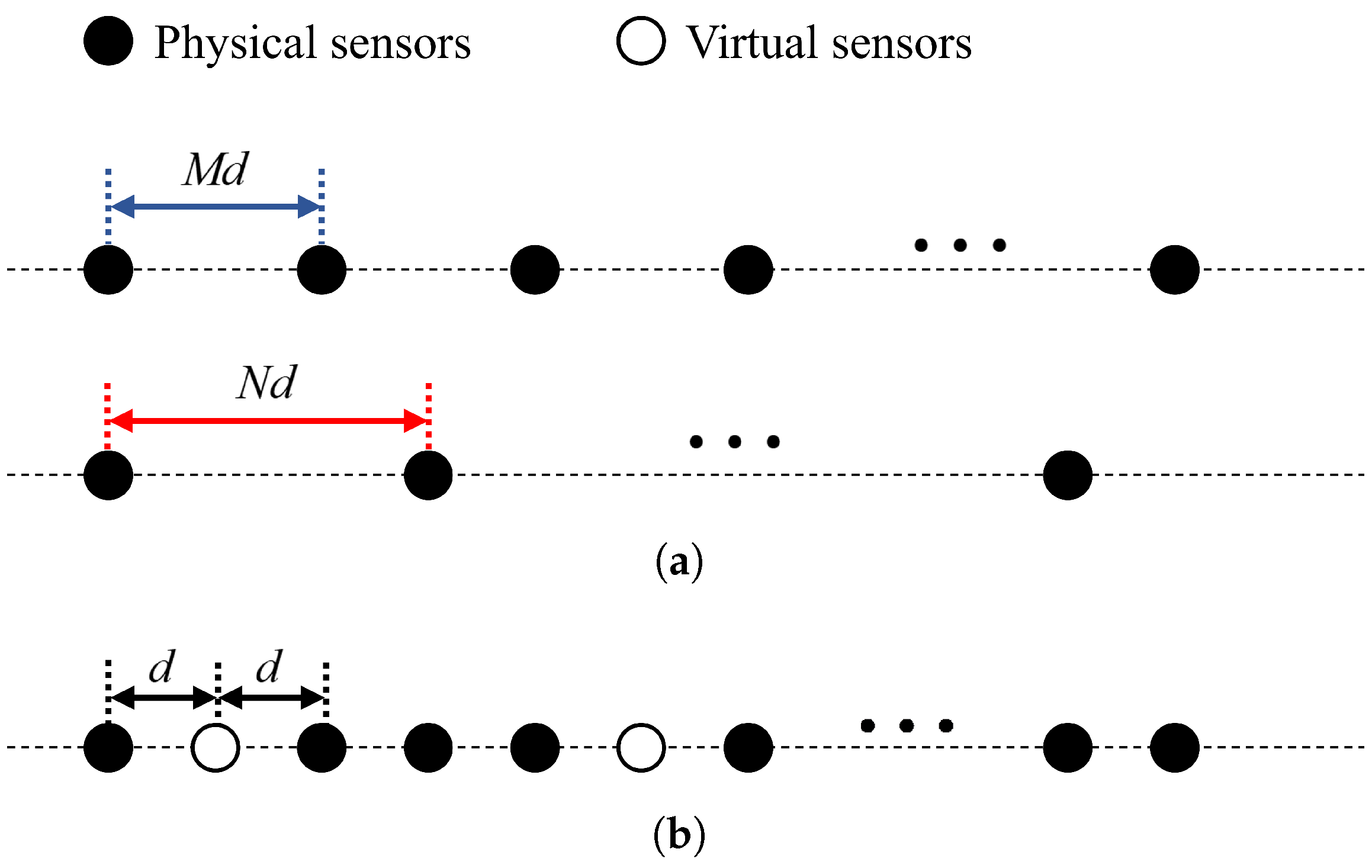
The coprime array configuration integrates two sparse ULAs as depicted in Figure 1a. The sensor elements are strategically located at and within the respective ULAs. Specifically, the first ULA comprises N elements with an inter-element spacing of , while the second ULA consists of M elements with an inter-element spacing of , where M and N are coprime integers. The coprime nature of M and N ensures that the two ULAs have a single overlap point at the origin. For generality, we assume . The inter-element spacing d is set to half the carrier wavelength, i.e., , where denotes the carrier wavelength. Consequently, the coprime array is composed of physical sensors, with the sensor positions given by , where , forming a discrete integer set:
which represents a non-uniform linear sparse array with sensors, where denotes the cardinality of the set. Thus, the effective aperture of the array is determined by .
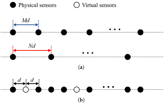
Figure 1.
Illustration of array configurations. (a) Non-uniform coprime array configurations; (b) The interpolated array.
Considering a narrowband SOI and narrowband interference signals. The DOA for the signal and interference are , and the observation vector of the array can be mathematically expressed as follows:
the observation vector of the array, which at time k can be decomposed into components corresponding to the SOI, interference, and noise. Specifically, represents the SOI component, represents the interference component, where is the steering vector associated with the l-th source, and represents the noise component. Here, denotes the waveform of the l-th source signal, and is the steering vector associated with the l-th source. The steering vector of a coprime array with respect to different directions is defined as follows,
where . The noise components are modeled as independent and identically distributed (i.i.d.) additive white Gaussian noise, expressed as , where denotes the noise power and is the identity matrix of the appropriate dimensions.
Utilizing adaptive beamforming techniques in coprime arrays effectively removes interference. The resulting output of the adaptive beamformer can be represented as
where the beamformer weight vector is utilized to define the output SINR for the coprime array. The SINR for this configuration is mathematically expressed as follows:
where the parameter denotes the power of the SOI, while represents the INCM, defined as
where denotes the power of the l-th interference.
To maximize the SINR, it is essential to ensure a distortion-free response of the SOI while minimizing the output power of interference and noise. Consequently, the SINR maximization optimization problem in (4) can be transformed into an interference and noise minimization problem, expressed as follows:
By solving this optimization problem using the Lagrange multiplier method, the optimal weight vector is determined as follows:
In practical scenarios, obtaining the theoretical is challenging. Therefore, it is typically estimated using the sample covariance matrix (SCM), which is calculated directly from the received signal. The SCM for snapshots is obtained by the following equation:
The beamformer (7) can be reformulated as the SMI beamformer:
which is the SCM beamformer, and is closely related to the steering vector of the SOI. Therefore, any inaccuracies in the steering vector obtained from the actual coprime array can affect the performance of the beamformer. However, there is a notable discrepancy between the SCM and the INCM. Therefore, this paper focuses on accurately estimating the INCM and the ideal signal steering vector from the received signals in the coprime array.
2.2. Coprime Array Interpolation Algorithm
Coprime array interpolation entails placing extra sensors into the ’holes’ at positions that are integer multiples of half-wavelengths, where no physical sensors are present in the coprime array .
Vectorizing yields a new vector
where , with for , , and
where is a column vector with all elements zero except for a one at the i-th position. The vector represents the received data from the virtual array extending the resonant aperture, and its corresponding steering vector is denoted as . The sensor positions of this virtual array can all be described by integers in the set . Nevertheless, the virtual source signal reduces to a single snapshot of , and constitutes a constant vector.
Vector has some duplicate items, and by eliminating them and reordering them we obtain a new vector ,
where represents the co-array matrix of . Specifically, .
According to the properties of coprime numbers, the resulting difference co-array is not an ideal ULA, meaning the integer indices are not a continuous sequence of integers and there are ’holes’. Therefore, algorithms that derive the covariance matrix of the virtual array, such as spatial smoothing, cannot directly use the array output . To address this issue, an interpolated vector is constructed as
where , .
It is important to note that the interpolated sensors exist mathematically rather than physically. Consequently, the received signals associated with these interpolated sensors should be regarded as unknown.
Given that is Hermitian symmetric, it follows that is also Hermitian symmetric [55], i.e.,
where and .
Notably, the theoretical covariance matrix for the uncorrelated signals received by the ULA exhibits a Hermitian Toeplitz structure. This characteristic can be leveraged as prior information for structured matrix recovery. Utilizing the properties of the vector , the resulting Hermitian Toeplitz matrix is given by
where represents the subset of containing non-negative integers.
The presence of zero elements in indicates corresponding zero elements in , necessitating the recovery of this missing information. The covariance matrix features a Hermitian Toeplitz structure. Furthermore, because the number of incident sources is relatively small compared to the dimension of the covariance matrix, the noise-free covariance matrix exhibits low-rank characteristics. Given these conditions, the interpolated ULA covariance matrix can be recovered by solving the following optimization problem:
where . The goal of the aforementioned optimization problem is to retrieve the low-rank Hermitian PSD Toeplitz covariance matrix of the interpolated ULA. This is done by ensuring that the corresponding elements of the sample covariance matrix match those of the recovered covariance matrix . However, (15) represents a non-convex NP-hard problem. By applying a nuclear norm convex relaxation, the optimization function can be reformulated as
The optimization problem (16) is convex and can be effectively addressed using interior point methods. For clarity, the covariance matrix reconstruction algorithm based on coprime array interpolation is outlined in Algorithm 1 below:
| Algorithm 1: Covariance matrix reconstruction based on coprime array interpolation |
|
2.3. Pre-Estimated INCM
For accurate INCM estimation, this paper employs an efficient reconstruction method grounded in the Capon spatial spectrum. The INCM is determined by integrating across an angular range that excludes the desired signal’s direction. By reintroducing the MVDR beamformer (9) into the objective function (6), the Capon spatial spectrum is derived as
To enhance the precision of , we first reconstruct the coprime array covariance matrix using Equation (16). This reconstructed matrix is subsequently substituted into Equation (17) to refine the results. Additionally, the steering vector originally associated with should be replaced with the steering vector corresponding to the interpolated ULA. Consequently, the Capon spatial spectrum can be reformulated as follows:
where . At this stage, serves as an approximation for the Capon spatial spectrum of the ULA. Following this, the INCM is reconstructed by integrating the Capon spatial spectrum.
where the integral range of the angle, , includes only the angles of the interference signals, excluding the SOI signal. includes all the information about interference and noise and is not affected by the SOI. However, conventional integration methods lead to a sharp increase in computational complexity, necessitating the adoption of an efficient solution method. Therefore, the integral operation can be approximately simplified into a discrete form [36]. In other words, the integration can be approximated by summation as follows:
where the original integral range is discretized into L angles within . To simplify the notation, is written as . The precision of the approximate integral expression increases with the number of discretized angles L. Additionally, the computational complexity of this approach is .
Nonetheless, the estimated is obtained from , which includes data related to the desired signal. Additionally, through summation poses problems that need urgent resolution. To accurately approximate the integral operation, a large number of discretized angles L are required, resulting in significant computational complexity.
2.4. INCM Reconstruction
In this section, an adaptive beamforming algorithm for coprime arrays is introduced, leveraging INCM reconstruction. Initially, the method employs a projection matrix to remove the SOI from the received signals. The projection matrix-processed approximate covariance matrix will then replace in Equation (20). Then, to reduce computational complexity, a GLQ algorithm is introduced to propose a new matrix reconstruction method as an alternative to the integral operation. Finally, the steering vector is updated by maximizing the beamformer’s output power, addressing the model mismatch issue.
The goal is to achieve . Furthermore, the function of the projection matrix is to extract the signal that only contains from the received signal . This reduces the impact of the desired signal on the INCM, resulting in a more accurate INCM. First, a pseudo-covariance matrix is constructed as
where is a construction parameter. The value of affects the orthogonality between the constructed matrix and the desired signal and should be chosen to be relatively large. In the simulations of this paper, is set to . In practical applications, to reduce computational load, should be set to . can be expressed in terms of its eigenvalues and eigenvectors, with the eigenvalues arranged in descending order, as follows:
where and for , . The eigenvectors correspond to the eigenvalues . Consequently, the inverse of the constructed pseudo-covariance matrix is given by
Based on the condition being satisfied and considering , can be approximated as
According to the mathematical derivation, can serve as the projection matrix , which is given by
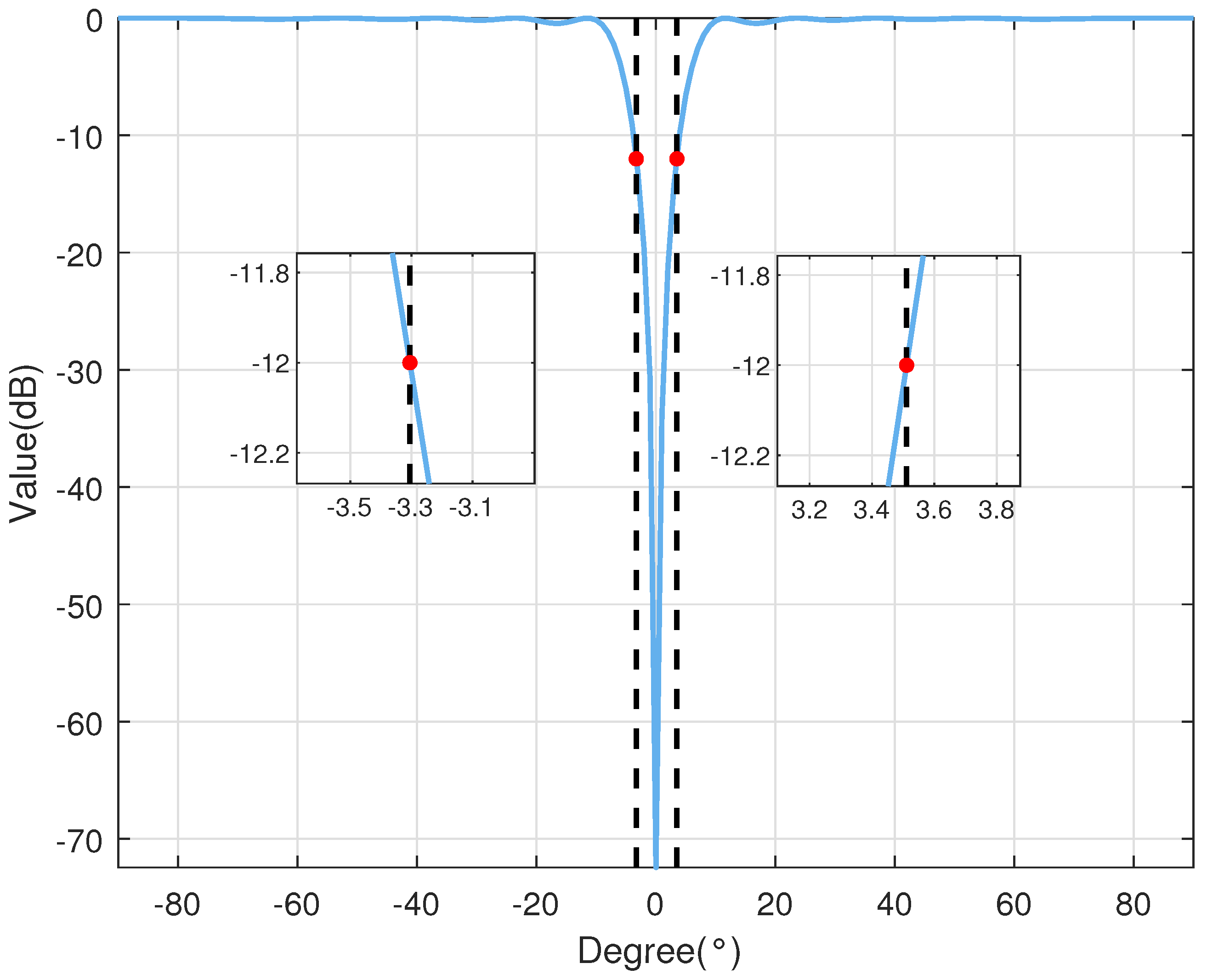
Figure 2 illustrates the function as it varies with . In practical applications, a 12 dB threshold is commonly used for signal detection. When the signal is below 12 dB, it is evident that the projection matrix can effectively remove the target signal. This is true even in the presence of certain angular errors, where the matrix still maintains its signal elimination capability. In this scenario, a coprime array with and is examined. The desired signal comes from , while three interferers originate from , , and . Each interferer has a signal-to-noise ratio (SNR) and interference-to-noise ratio (INR) of 20 dB. As illustrated in Figure 2, when aligns with the desired signal direction , is significantly reduced. Hence, the SOI is effectively suppressed.
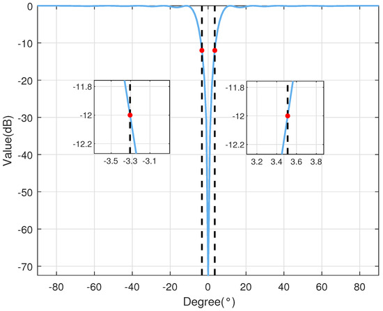
Figure 2.
The value of as a function of .
Next, a covariance matrix processed by the projection matrix can be obtained. In this covariance matrix, the SOI information is eliminated, retaining only the interference and noise information, as follows:
Here, denotes the estimated noise power, which is commonly derived from the smallest eigenvalue of . By substituting in Equation (20) with , we obtain
The quadrature formula with L discrete points, also known as the mechanical quadrature formula, is used for numerical integration. When the discrete points for integration are equally spaced, using L nodes can approximate the integration accuracy up to the ()-th order. Nodes that achieve this level of accuracy are referred to as Gaussian points, and the quadrature formula that attains this accuracy is known as the Gaussian quadrature formula. Currently, the Gaussian quadrature formula is the most accurate quadrature formula available.
The necessary and sufficient condition for nodes to be Gaussian points is that the polynomial having these nodes as its zeros must be orthogonal to any polynomial of degree not exceeding over the interval . That is,
for all polynomials of degree not exceeding , where is the polynomial having the Gaussian points as its zeros.
In practical applications of numerical integration, computational complexity is a critical evaluation criterion. The computational complexity of the trapezoidal rule is , requiring evaluations of the function to complete the integration. Similarly, Simpson’s rule has a computational complexity of , also requiring function evaluations. However, despite having the same computational complexity, both methods require a large number of nodes to achieve high accuracy, significantly increasing the computational load. In contrast, the Gauss–Legendre quadrature (GLQ) method also has a computational complexity of , but due to its high polynomial accuracy, it can achieve the same precision with fewer nodes. For example, to achieve an accuracy of , the trapezoidal rule may need thousands of nodes, Simpson’s rule may require hundreds of nodes, whereas GLQ may only need around 10 nodes or fewer. Therefore, to achieve an optimal balance between computational complexity and accuracy, the GLQ method is the most efficient choice.
The N-th standard Legendre polynomial is expressed as
where it is orthogonal to any polynomial of degree not exceeding over the interval , and all its distinct roots lie within the interval . Therefore, the N zeros of the Legendre polynomial can be used as the Gaussian points for the Gaussian quadrature formula.
To mitigate the problem of increasing computational complexity in solving (27) as the number of discretizations L grows, this paper introduces an effective matrix reconstruction technique utilizing the GLQ. GLQ, which is the Gaussian quadrature formula using the Legendre polynomials, is a highly accurate method for numerical integration, known for its algebraic precision. When the integrand is polynomial, GLQ provides a precise approximation. The generalized interpolatory Gaussian quadrature is formulated as
where are the Gaussian quadrature nodes, and and represent the lower and upper limits of the integration, respectively. represents the error between the actual value of the integral and its approximation.
are the weights, calculated as follows:
Here, is a polynomial in q. According to Gauss’s theorem, must be orthogonal to any polynomial of lower degree than N.
For ease of computation, the nodes of the Gaussian quadrature in (29) are chosen to be the roots of , which are used to construct the GLQ. To balance computational complexity and algebraic accuracy, this paper employs third-order GLQ to calculate the integral [45]. The Gaussian integration nodes required for third-order GLQ are determined by , i.e., , , and .
The integration interval is conveniently chosen as . Therefore, (29) is rewritten as
Let in (30), and the resulting weights are
Using the third-order Legendre polynomial, the weights are obtained as , , and . Combining the roots and weights of the third-order Legendre polynomial and substituting them into (31), we obtain
And by using a linear transformation of the integral, the third-order GLQ can be generalized to a general integral as
where Therefore, the third-order GLQ can also be used to compute the INCM (27) as
where and the integral range is given by . It should be noted that the integration range represents the interference range.
By obtaining from (35), which excludes the desired signal information, and substituting it into (20) in place of , the output power of the beamformer can be expressed as
In the Capon spatial spectrum, the peak position corresponds to the DOA estimate of the desired signal. Furthermore, the steering vector of the SOI can be estimated as .
Substituting the reconstructed INCM and to (9), we obtain
The obtained beamformer, combined with the corresponding channel information, can achieve good anti-interference performance. Based on the previous discussion, Algorithm 2 outlines the steps for implementing the proposed robust adaptive beamforming algorithm for coprime arrays.
| Algorithm 2: The implementation process of the proposed robust adaptive beamforming |
|
2.5. Algorithm Performance Analysis
The computational complexity of the proposed robust beamforming algorithm is mainly determined by the construction of the projection matrix, INCM reconstruction, and spectral peak search. However, the INCM reconstruction based on GLQ requires only three additions, resulting in very low computational complexity. Therefore, the primary factors affecting the computational complexity are the construction of the projection matrix and the spectral peak search. The construction of the projection matrix requires obtaining the eigenvalues and eigenvectors of as described in (23). The eigen decomposition of is the primary factor affecting the computational complexity, with a complexity of . The computational burden for the spectral peak search is , where P represents the number of grid points in the angular domain. Therefore, the overall complexity of the algorithm is approximately .
3. Simulation and Experimental Results
The effectiveness of the proposed algorithm is verified through simulation and experimental results. In the example of this section, we assume a coprime array with coprime integers 3 and 5, i.e., . This means that the sensor array consists of physical sensors. Assume the SOI impinges on the array from , and three interferers come from , , and , respectively. In all simulation experiments, the INR of each interferer is set to 30 dB. When the experiment studies the impact of input SNR variation on SINR, the number of snapshots is fixed at . When the experiment studies the impact of snapshot number variation on SINR, the input SNR is fixed at 20 dB. Each figure represents the results of 500 Monte Carlo experiments. The performance of the proposed beamformer is evaluated in comparison to the following beamformers:
- (i)
- integration beamformer [47];
- (ii)
- summation beamformer [47];
- (iii)
- coprime co-array interpolation beamformer [60];
- (iv)
- reconstruction-based beamformer [35];
- (v)
- worst-case SINR maximization beamformer [34].
We assume the angular sector of the SOI is , then .
3.1. Example 1: Known Signal Steering Vector
In the first example, we examine the scenario where the steering vector of the input signal is known. It is worth noting that, due to the presence of SOI information in the snapshots, the adaptive beamformer is still affected, leading to a performance degradation.
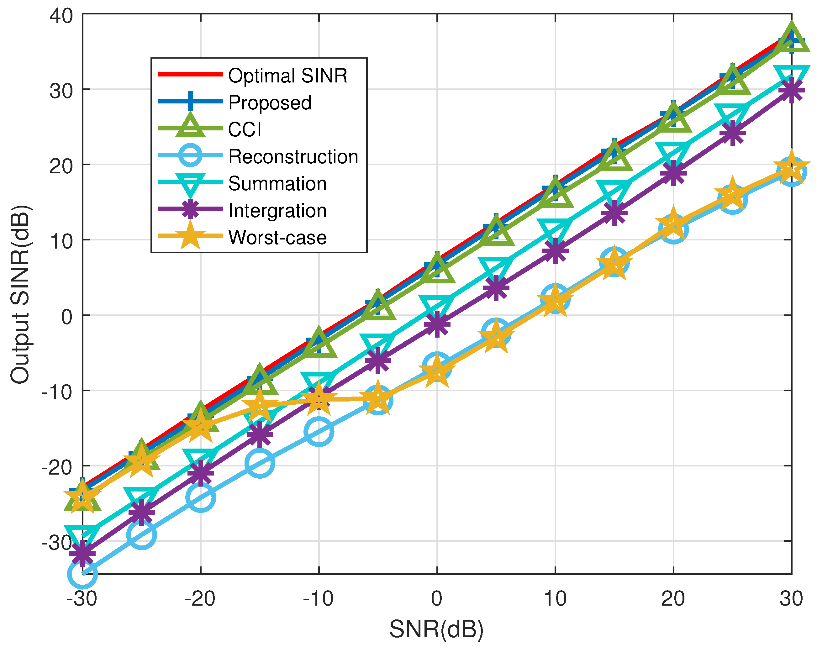
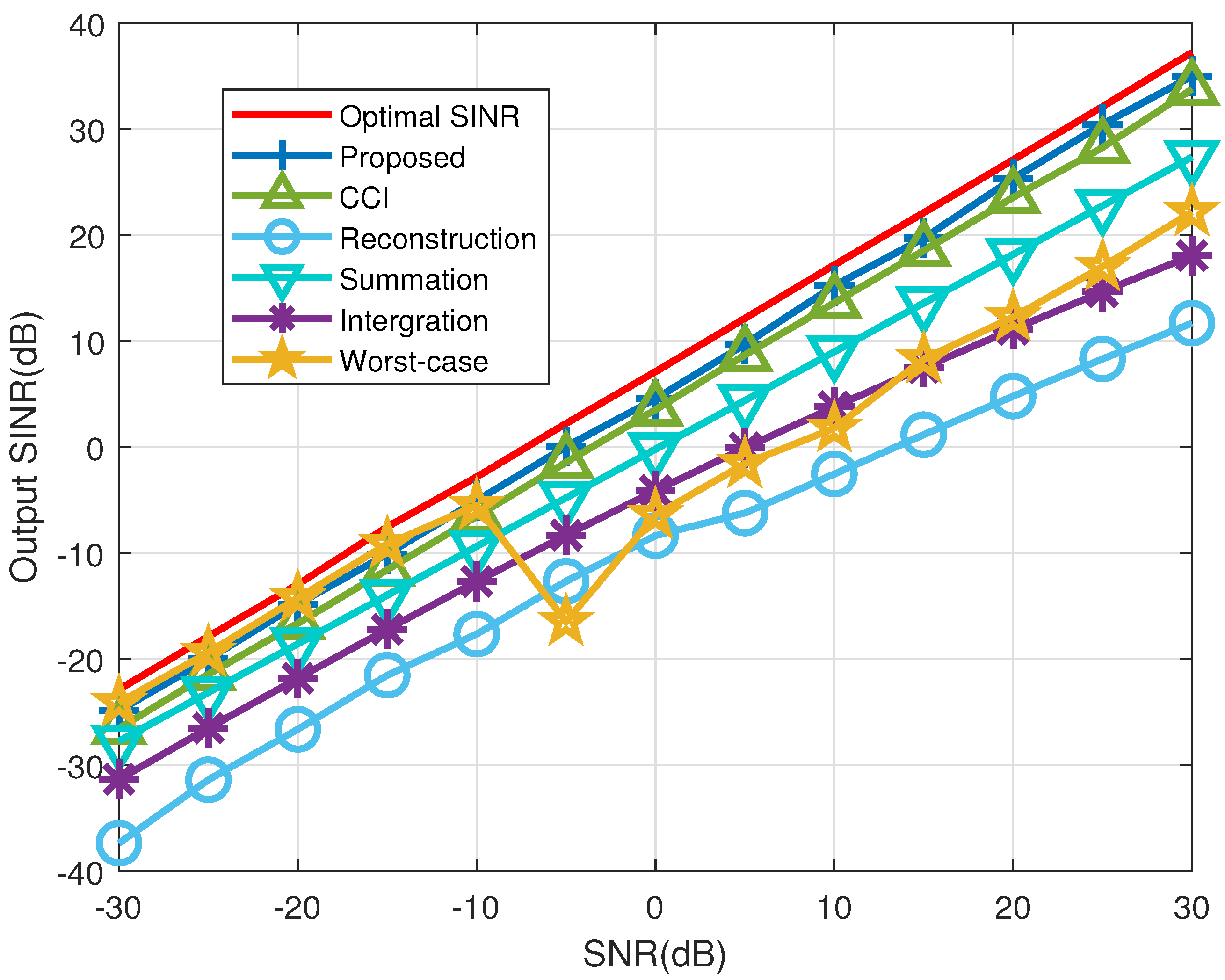
The relationship between the output SINR of the beamformer and the input SNR is shown in Figure 3. From this figure, we can intuitively see that the proposed beamformer achieves nearly optimal SINR within the range of -30 dB to 30 dB when the signal steering vector is known. Furthermore, it outperforms all other beamformers compared within the defined SNR range.

Figure 3.
Output SINR versus input SNR in example 1 (Snapshots: 50, INR: 30 dB).
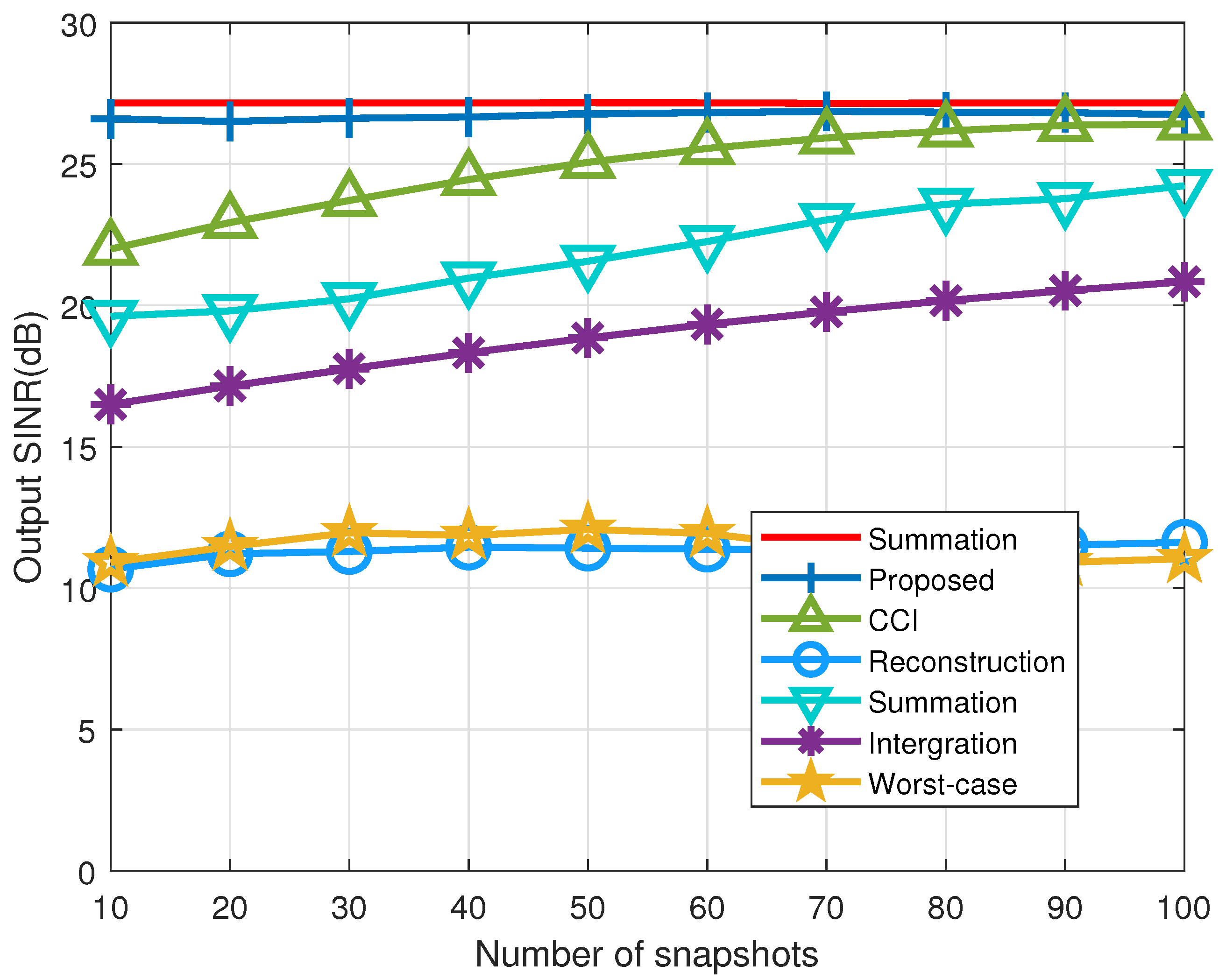
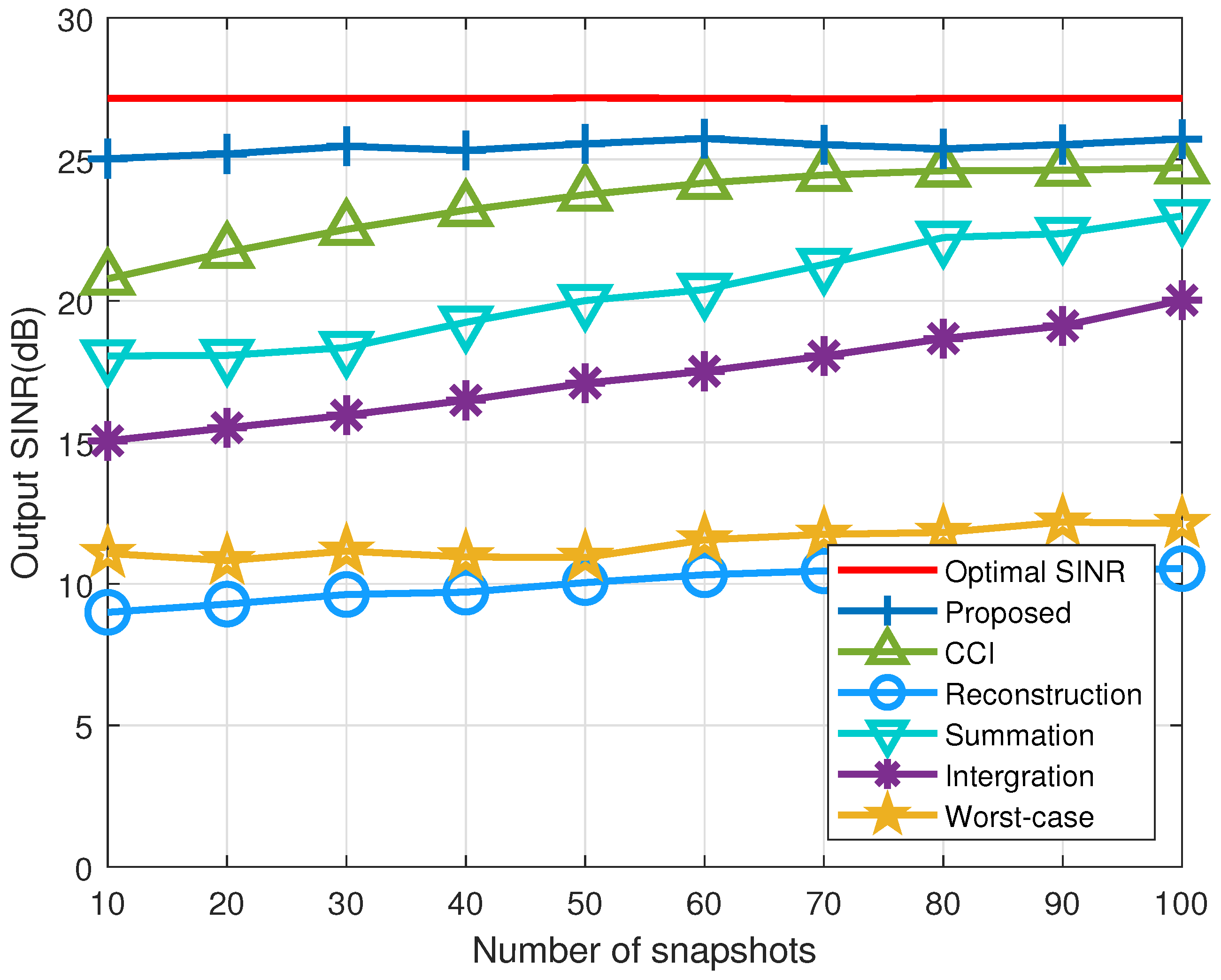
The beamformer based on coprime co-array interpolation also performs well within the defined SNR range. However, because the SOI is not completely removed within the snapshots, its performance is somewhat lacking compared to the proposed beamformer. Based on the worst-case beamformer, the performance is close to that of the optimal beamformer under low SNR conditions. However, its performance degrades at high SNR because the covariance matrix used does not effectively remove the SOI information. The proposed beamformer surpasses existing beamformers by fundamentally removing the SOI information through the application of a projection matrix. This approach enables the construction of a more precise INCM. The relationship between the output SINR of the beamformer and the number of snapshots is shown in Figure 4. It is evident that as the number of snapshots varies from 10 to 100, the proposed beamformer consistently outperforms the other beamformers, demonstrating particularly superior performance at lower snapshot numbers.
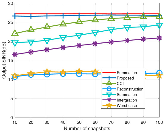
Figure 4.
Output SINR versus the number of snapshots in example 1 (SNR: 20 dB, INR: 30 dB).
3.2. Example 2: Mismatch Due to Signal Look Direction Error
In the second example, the effect of signal and interference DOA mismatch on the beamformer’s performance is examined. Assume the random DOA errors of the input signals are uniformly distributed within . Furthermore, the actual DOA of the SOI is distributed within , and the DOAs of the interferers are distributed within , , and , respectively. In each Monte Carlo simulation, the DOA of the input signals changes but stays constant for the same set of snapshots during an experiment.
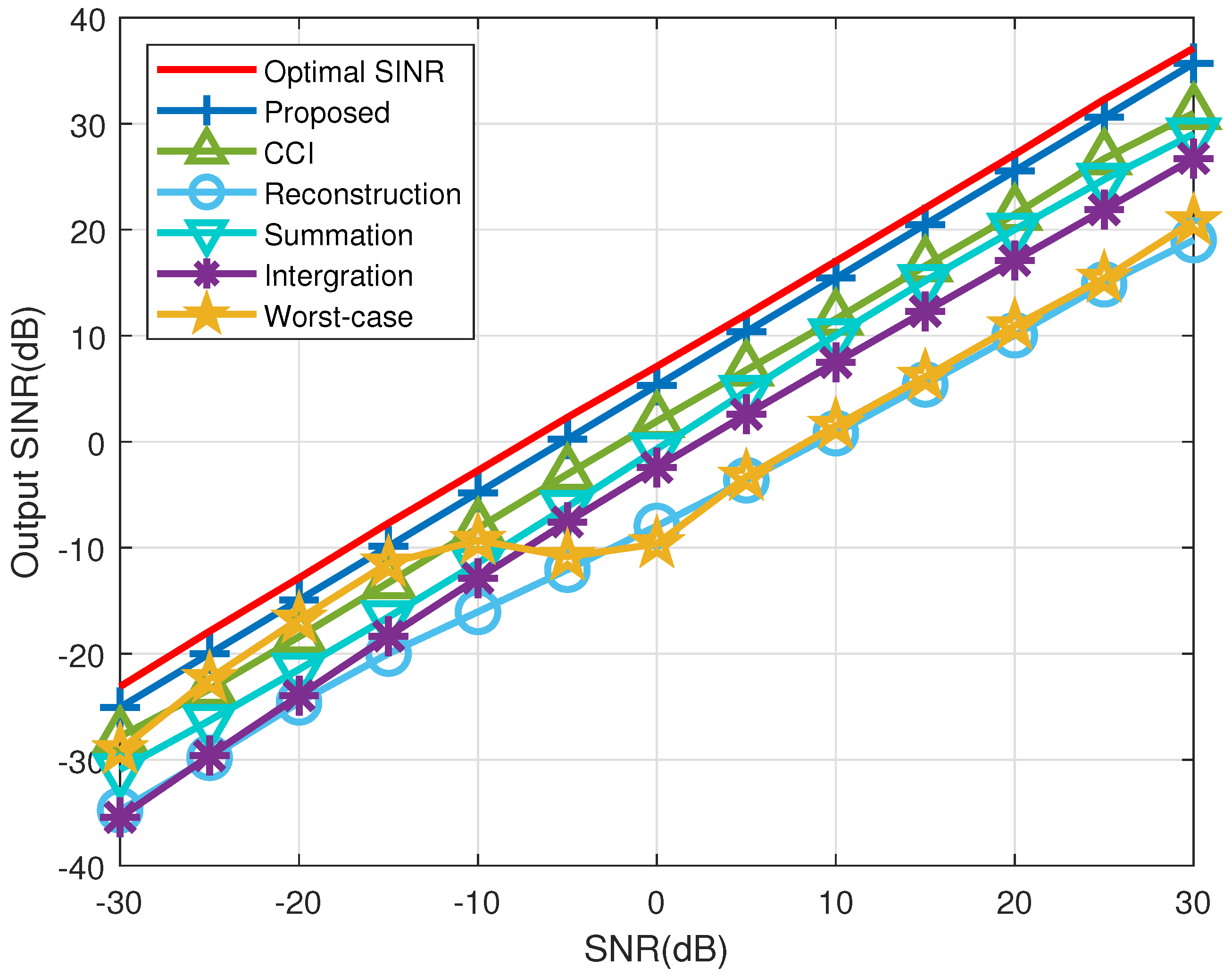
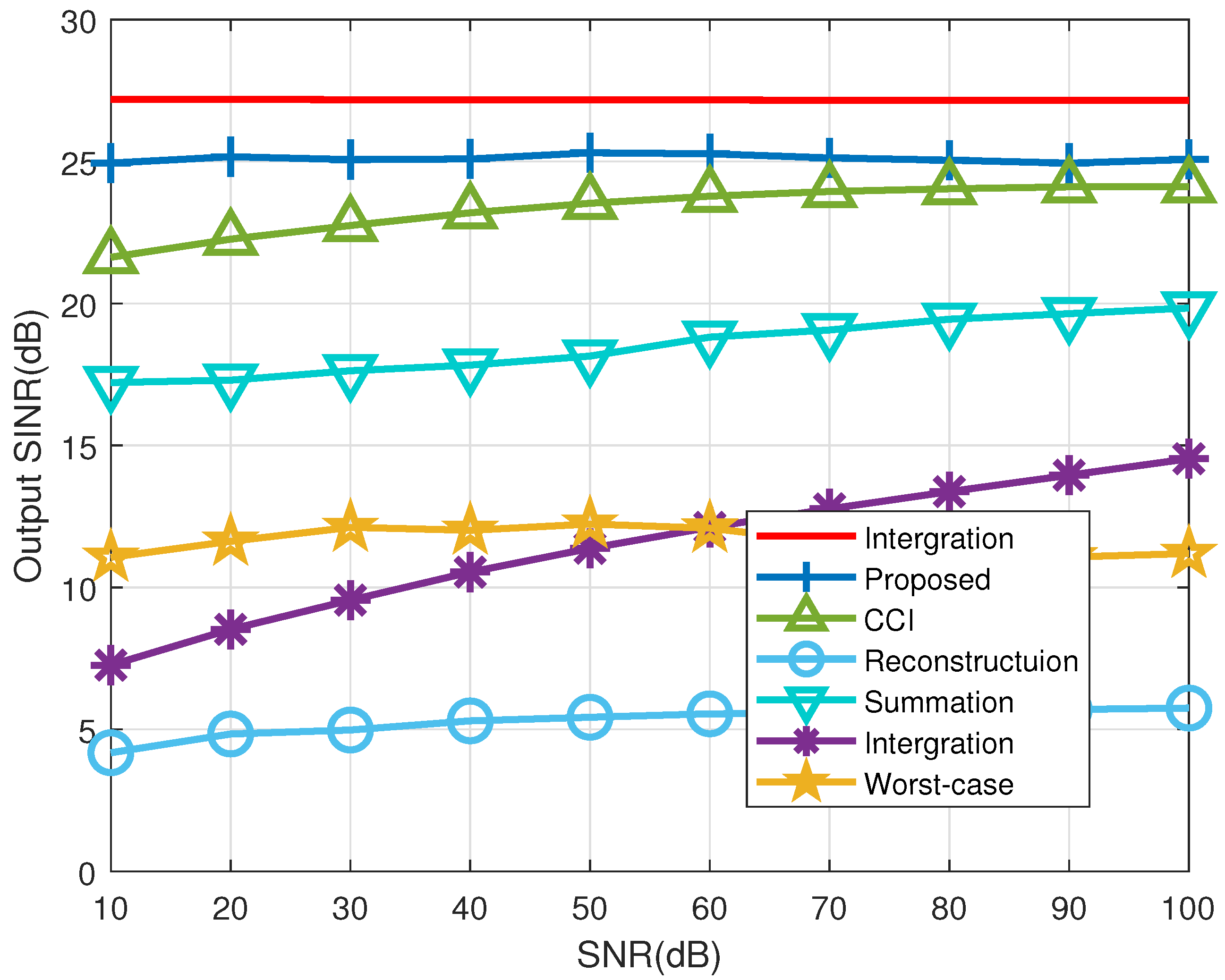
Figure 5 presents the output SINR of the evaluated beamformers as a function of the SNR. It is clear that both the proposed beamformer and the coprime co-array interpolation beamformer operate effectively within the specified SNR range. Additionally, the proposed beamformer surpasses the coprime co-array interpolation beamformer due to its superior INCM reconstruction accuracy. The worst-case beamformer performs well at low SNR but its performance degrades at high SNR. The correlation between the beamformer’s output SINR and the number of snapshots is illustrated in Figure 6. The proposed beamformer demonstrates better performance compared to other algorithms, particularly in the range of 10 to 100 snapshots, with a more notable advantage at lower snapshot counts.
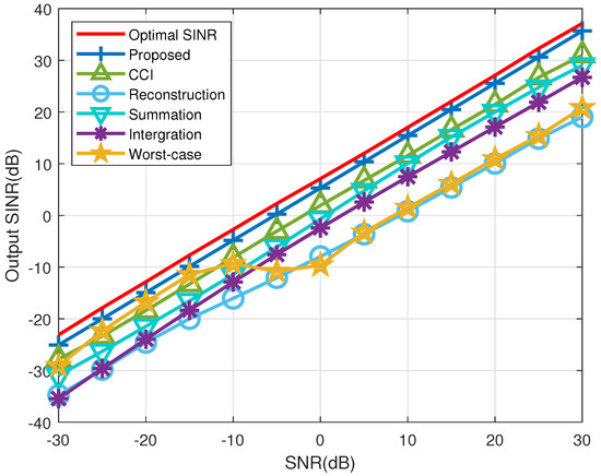
Figure 5.
Output SINR versus input SNR in example 2 (Snapshots: 50, INR: 30 dB).
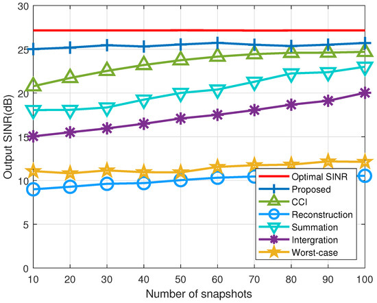
Figure 6.
Output SINR versus the number of snapshots in example 2 (SNR: 20 dB, INR: 30 dB).
3.3. Example 3: Gain and Phase Mismatch
The third example examines how gain and phase mismatches affect beamformer performance. The amplitude and phase error of the i-th sensor is
where denotes the gain variation at the i-th sensor, characterized by a zero mean and randomness, and denotes the phase variation at the same sensor, also random with a zero mean.
Figure 7 shows the relationship between the input SNR and the SINR of the beamformer, and Figure 8 shows the relationship between the number of snapshots used to generate the SCM from the received signals and SINR of the resulting beamformer. The worst-case beamformer exhibits superior performance compared to the other beamformers under low SNR conditions. However, its performance deteriorates at high SNR. In Figure 7, it can be seen that the proposed beamformer performs well even in the presence of gain and phase perturbation mismatches, and it is the closest to the optimal performance. Figure 8 shows that the proposed algorithm nearly achieves optimal performance with fewer snapshots and surpasses other existing methods.
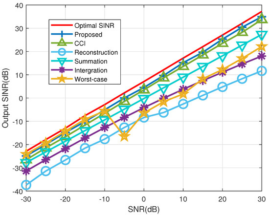
Figure 7.
Output SINR versus input SNR in example 3 (Snapshots: 50, INR: 30 dB).
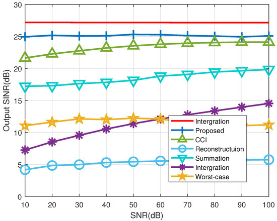
Figure 8.
Output SINR versus the number of snapshots in example 3 (SNR: 20 dB, INR: 30 dB).
4. Discussion
The simulation results presented in Section 3 demonstrate the robustness and effectiveness of the proposed beamformer under various conditions, including known signal steering vectors, DOA mismatches, and gain and phase mismatches. These scenarios are critical in practical applications where perfect knowledge of the environment is often unattainable.
When the steering vector of the SOI is known, the proposed beamformer achieves nearly optimal performance across a wide range of SNR values, consistently outperforming other methods. This highlights the algorithm’s ability to accurately reconstruct the INCM by effectively eliminating the SOI component through projection matrices.
In the presence of DOA mismatches, the proposed beamformer still maintains superior performance compared to other beamformers. The improved INCM reconstruction accuracy accounts for this robustness, making the algorithm suitable for environments where signal and interference directions are not perfectly known.
In applying the GLQ method for power spectrum integration to obtain the covariance matrix, gain and phase mismatches significantly affect the numerical integration accuracy, leading to performance degradation. Gain mismatch implies that the actual values of the integrand function deviate from the true values due to measurement inaccuracies, data noise, or model imperfections. As GLQ nodes and weights are designed for ideally smooth functions, these errors accumulate directly at each node, causing the overall integration result to deviate from the true value. Additionally, for power spectra with significant variations, gain mismatch amplifies because GLQ nodes might fall within regions of large errors, further exacerbating the integration inaccuracy.
Phase mismatch affects the phase component of the power spectrum, which is critical in calculating the covariance matrix, such as in the term . Phase mismatch causes deviations in these phase relationships, leading to systematic biases in the integration results and introducing periodic disturbances. These disturbances result in additional oscillatory terms in the integration result, further reducing accuracy. Therefore, in the presence of gain and phase mismatches, the performance of the GLQ method significantly degrades, highlighting the need for careful consideration of these error sources in practical applications.
5. Conclusions
This paper proposes a novel robust adaptive beamforming algorithm for coprime arrays based on URG. In contrast to existing methods, this approach expands the array’s effective aperture via coprime array interpolation and efficiently removes SOI information using a projection matrix, thus allowing for a more precise INCM reconstruction. To reduce the computational complexity of the algorithm, GLQ is introduced. Compared with existing algorithms, this method exhibits greater robustness in scenarios with known steering vectors, DOA mismatches between signals and interferers, and gain and phase perturbation mismatches. Simulation results show that the proposed beamformer achieves superior performance with less computational effort compared to other beamformers and consistently remains close to optimal. Additionally, the algorithm outperforms existing methods, particularly with fewer snapshots. Future work will investigate novel INCM reconstruction techniques aimed at increasing the beamformer’s robustness and decreasing computational complexity.
Author Contributions
Conceptualization, S.C. and X.Z.; methodology, S.C.; software, S.C.; validation, S.C., X.Z. and X.W.; formal analysis, S.C.; investigation, S.C.; resources, S.C.; data curation, S.C.; writing—original draft preparation, S.C.; writing—review and editing, S.C.; visualization, S.C.; supervision, X.Z.; project administration, X.Z.; funding acquisition, X.Z., S.L. and W.D. contributed to the validation and review processes. All authors have read and agreed to the published version of the manuscript.
Funding
This work was supported in part by the National Natural Science Foundation of China under Grant 61701140, and research project fund of Songjiang Laboratory (No. SL20230204).
Data Availability Statement
Data are contained within the article.
Conflicts of Interest
The authors declare no conflicts of interest.
Abbreviations
The following abbreviations are used in this manuscript:
| ULAs | Uniform Linear Arrays |
| DOF | Degrees of Freedom |
| DOA | Direction-of-arrival |
| INCM | Interference-plus-Noise Covariance Matrix |
| MVDR | Minimum Variance Distortionless Response |
| SOI | Signal of Interest |
| NLAs | Non-Uniform Linear Arrays |
| SCM | Sample Covariance Matrix |
| GLQ | Gauss–Legendre Quadrature |
| URG | Unwanted Signal Removal and Employs Gauss–Legendre Quadrature |
| SMI | Sample Matrix Inversion |
| CCI | Coprime Coarray Interpolation |
| SINR | Signal-to-Interference-plus-Noise Ratio |
| SNR | Signal-to-Noise Ratio |
| INR | Interference-to-Noise Ratio |
References
- Fabrizio, G.A.; Gershman, A.B.; Turley, M.D. Robust adaptive beamforming for HF surface wave over-the-horizon radar. IEEE Trans. Aerosp. Electron. Syst. 2004, 40, 510–525. [Google Scholar] [CrossRef]
- Li, J.; Stoica, P. Robust Adaptive Beamforming; John Wiley & Sons: Hoboken, NJ, USA, 2005. [Google Scholar]
- Xiang, C.; Feng, D.Z.; Lv, H.; He, J.; Cao, Y. Robust adaptive beamforming for MIMO radar. Signal Process. 2010, 90, 3185–3196. [Google Scholar] [CrossRef]
- Xu, J.; Liao, G.; Huang, L.; So, H.C. Robust adaptive beamforming for fast-moving target detection with FDA-STAP radar. IEEE Trans. Signal Process. 2016, 65, 973–984. [Google Scholar] [CrossRef]
- Lin, Z.; Chen, Y.; Liu, X.; Jiang, R.; Shen, B. Adaptive beamforming design of planar arrays based on Bayesian compressive sensing. IEEE Sens. J. 2020, 21, 5185–5194. [Google Scholar] [CrossRef]
- Liu, C.; Li, M.; Zhao, L.; Whiting, P.; Hanly, S.V.; Collings, I.B.; Zhao, M. Robust adaptive beam tracking for mobile millimetre wave communications. IEEE Trans. Wirel. Commun. 2020, 20, 1918–1934. [Google Scholar] [CrossRef]
- Chang, S.; Deng, Y.; Zhang, Y.; Zhao, Q.; Wang, R.; Zhang, K. An advanced scheme for range ambiguity suppression of spaceborne SAR based on blind source separation. IEEE Trans. Geosci. Remote Sens. 2022, 60, 5230112. [Google Scholar] [CrossRef]
- Huang, Y.; Zhou, M.; Vorobyov, S.A. New designs on MVDR robust adaptive beamforming based on optimal steering vector estimation. IEEE Trans. Signal Process. 2019, 67, 3624–3638. [Google Scholar] [CrossRef]
- Yazdi, N.; Todros, K. Measure-transformed MVDR beamforming. IEEE Signal Process. Lett. 2020, 27, 1959–1963. [Google Scholar] [CrossRef]
- Shahbazpanahi, S.; Gershman, A.B.; Luo, Z.Q.; Wong, K.M. Robust adaptive beamforming using worst-case SINR optimization: A new diagonal loading-type solution for general-rank signal models. In Proceedings of the 2003 IEEE International Conference on Acoustics, Speech, and Signal Processing, 2003 (ICASSP’03), Hong Kong, China, 6–10 April 2003; Volume 5, p. V-333. [Google Scholar] [CrossRef]
- Elnashar, A.; Elnoubi, S.M.; El-Mikati, H.A. Further study on robust adaptive beamforming with optimum diagonal loading. IEEE Trans. Antennas Propag. 2006, 54, 3647–3658. [Google Scholar] [CrossRef]
- Lin, J.R.; Peng, Q.C.; Shao, H.Z. On Diagonal Loading for Robust Adaptive Beamforming Based on Worst-Case Performance Optimization. ETRI J. 2007, 29, 50–58. [Google Scholar] [CrossRef]
- Du, L.; Li, J.; Stoica, P. Fully automatic computation of diagonal loading levels for robust adaptive beamforming. IEEE Trans. Aerosp. Electron. Syst. 2010, 46, 449–458. [Google Scholar] [CrossRef]
- Zhang, M.; Chen, X.; Zhang, A. A simple tridiagonal loading method for robust adaptive beamforming. Signal Process. 2019, 157, 103–107. [Google Scholar] [CrossRef]
- Gao, J.; Zhen, J.; Lv, Y.; Guo, B. Beamforming technique based on adaptive diagonal loading in wireless access networks. Ad Hoc Netw. 2020, 107, 102249. [Google Scholar] [CrossRef]
- Yang, Y.; Xu, X.; Yang, H.; Li, W. Robust adaptive beamforming via covariance matrix reconstruction with diagonal loading on interference sources covariance matrix. Digit. Signal Process. 2023, 136, 103977. [Google Scholar] [CrossRef]
- Youn, W.S.; Un, C.K. Robust adaptive beamforming based on the eigenstructure method. IEEE Trans. Signal Process. 1994, 42, 1543–1547. [Google Scholar] [CrossRef]
- Choi, Y.H. Eigenstructure-based adaptive beamforming for coherent and incoherent interference cancellation. IEICE Trans. Commun. 2002, 85, 633–640. [Google Scholar]
- Huang, F.; Sheng, W.; Ma, X. Modified projection approach for robust adaptive array beamforming. Signal Process. 2012, 92, 1758–1763. [Google Scholar] [CrossRef]
- Huang, L.; Zhang, B.; Ye, Z. Robust adaptive beamforming using a new projection approach. In Proceedings of the 2015 IEEE International Conference on Digital Signal Processing (DSP), Singapore, 21–24 July 2015; pp. 1181–1185. [Google Scholar]
- Yi, S.; Wu, Y.; Wang, Y. Projection-based robust adaptive beamforming with quadratic constraint. Signal Process. 2016, 122, 65–74. [Google Scholar] [CrossRef]
- Yang, X.; Li, Y.; Liu, F.; Lan, T.; Long, T.; Sarkar, T.K. Robust adaptive beamforming based on covariance matrix reconstruction with annular uncertainty set and vector space projection. IEEE Antennas Wirel. Propag. Lett. 2020, 20, 130–134. [Google Scholar] [CrossRef]
- Guo, J.; Yang, H.; Ye, Z. A novel robust adaptive beamforming algorithm based on subspace orthogonality and projection. IEEE Sens. J. 2023, 23, 12076–12083. [Google Scholar] [CrossRef]
- Vorobyov, S.A.; Gershman, A.B.; Luo, Z.Q.; Ma, N. Adaptive beamforming with joint robustness against mismatched signal steering vector and interference nonstationarity. IEEE Signal Process. Lett. 2004, 11, 108–111. [Google Scholar] [CrossRef]
- Hassanien, A.; Vorobyov, S.A.; Wong, K.M. Robust adaptive beamforming using sequential quadratic programming: An iterative solution to the mismatch problem. IEEE Signal Process. Lett. 2008, 15, 733–736. [Google Scholar] [CrossRef]
- Vorobyov, S.A. Principles of minimum variance robust adaptive beamforming design. Signal Process. 2013, 93, 3264–3277. [Google Scholar] [CrossRef]
- Somasundaram, S.D.; Butt, N.R.; Jakobsson, A.; Hart, L. Low-complexity uncertainty-set-based robust adaptive beamforming for passive sonar. IEEE J. Ocean. Eng. 2015. Early Access. [Google Scholar] [CrossRef]
- Huang, L.; Zhang, J.; Xu, X.; Ye, Z. Robust adaptive beamforming with a novel interference-plus-noise covariance matrix reconstruction method. IEEE Trans. Signal Process. 2015, 63, 1643–1650. [Google Scholar] [CrossRef]
- Liao, B.; Guo, C.; Huang, L.; Li, Q.; Liao, G.; So, H.C. Robust adaptive beamforming with random steering vector mismatch. Signal Process. 2016, 129, 190–194. [Google Scholar] [CrossRef]
- Zhuang, J.; Shi, B.; Zuo, X.; Ali, A.H. Robust adaptive beamforming with minimum sensitivity to correlated random errors. Signal Process. 2017, 131, 92–98. [Google Scholar] [CrossRef]
- Liao, B.; Guo, C.; Huang, L.; Li, Q.; So, H.C. Robust adaptive beamforming with precise main beam control. IEEE Trans. Aerosp. Electron. Syst. 2017, 53, 345–356. [Google Scholar] [CrossRef]
- Feng, Y.; Liao, G.; Xu, J.; Zhu, S.; Zeng, C. Robust adaptive beamforming against large steering vector mismatch using multiple uncertainty sets. Signal Process. 2018, 152, 320–330. [Google Scholar] [CrossRef]
- Chen, P.; Yang, Y. An uncertainty-set-shrinkage-based covariance matrix reconstruction algorithm for robust adaptive beamforming. Multidimens. Syst. Signal Process. 2021, 32, 263–279. [Google Scholar] [CrossRef]
- Huang, Y.; Fu, H.; Vorobyov, S.A.; Luo, Z.Q. Robust adaptive beamforming via worst-case SINR maximization with nonconvex uncertainty sets. IEEE Trans. Signal Process. 2023, 71, 218–232. [Google Scholar] [CrossRef]
- Gu, Y.; Leshem, A. Robust adaptive beamforming based on interference covariance matrix reconstruction and steering vector estimation. IEEE Trans. Signal Process. 2012, 60, 3881–3885. [Google Scholar]
- Gu, Y.; Goodman, N.A.; Hong, S.; Li, Y. Robust adaptive beamforming based on interference covariance matrix sparse reconstruction. Signal Process. 2014, 96, 375–381. [Google Scholar] [CrossRef]
- Shen, F.; Chen, F.; Song, J. Robust adaptive beamforming based on steering vector estimation and covariance matrix reconstruction. IEEE Commun. Lett. 2015, 19, 1636–1639. [Google Scholar] [CrossRef]
- Yuan, X.; Gan, L. Robust adaptive beamforming via a novel subspace method for interference covariance matrix reconstruction. Signal Process. 2017, 130, 233–242. [Google Scholar] [CrossRef]
- Zheng, Z.; Zheng, Y.; Wang, W.Q.; Zhang, H. Covariance matrix reconstruction with interference steering vector and power estimation for robust adaptive beamforming. IEEE Trans. Veh. Technol. 2018, 67, 8495–8503. [Google Scholar] [CrossRef]
- Zhu, X.; Xu, X.; Ye, Z. Robust adaptive beamforming via subspace for interference covariance matrix reconstruction. Signal Process. 2020, 167, 107289. [Google Scholar] [CrossRef]
- Yang, H.; Wang, P.; Ye, Z. Robust adaptive beamforming via covariance matrix reconstruction under colored noise. IEEE Signal Process. Lett. 2021, 28, 1759–1763. [Google Scholar] [CrossRef]
- Li, H.; Geng, J.; Xie, J. Robust adaptive beamforming based on covariance matrix reconstruction with RCB principle. Digit. Signal Process. 2022, 127, 103565. [Google Scholar] [CrossRef]
- Yang, H.; Ye, Z. Robust adaptive beamforming based on covariance matrix reconstruction via steering vector estimation. IEEE Sens. J. 2022, 23, 2932–2939. [Google Scholar] [CrossRef]
- Ge, S.; Fan, C.; Wang, J.; Huang, X. Robust adaptive beamforming based on sparse Bayesian learning and covariance matrix reconstruction. IEEE Commun. Lett. 2022, 26, 1893–1897. [Google Scholar] [CrossRef]
- Luo, T.; Chen, P.; Cao, Z.; Zheng, L.; Wang, Z. URGLQ: An efficient covariance matrix reconstruction method for robust adaptive beamforming. IEEE Trans. Aerosp. Electron. Syst. 2023, 59, 5634–5645. [Google Scholar] [CrossRef]
- Liu, C.L.; Vaidyanathan, P. Super nested arrays: Linear sparse arrays with reduced mutual coupling—Part I: Fundamentals. IEEE Trans. Signal Process. 2016, 64, 3997–4012. [Google Scholar] [CrossRef]
- Zhou, C.; Shi, Z.; Gu, Y. Coprime array adaptive beamforming with enhanced degrees-of-freedom capability. In Proceedings of the 2017 IEEE Radar Conference (RadarConf), Seattle, WA, USA, 8–12 May 2017; pp. 1357–1361. [Google Scholar]
- Zheng, Z.; Wang, W.Q.; Kong, Y.; Zhang, Y.D. MISC array: A new sparse array design achieving increased degrees of freedom and reduced mutual coupling effect. IEEE Trans. Signal Process. 2019, 67, 1728–1741. [Google Scholar] [CrossRef]
- Wagner, M.; Park, Y.; Gerstoft, P. Gridless DOA estimation and root-MUSIC for non-uniform linear arrays. IEEE Trans. Signal Process. 2021, 69, 2144–2157. [Google Scholar] [CrossRef]
- Pal, P.; Vaidyanathan, P.P. Nested arrays: A novel approach to array processing with enhanced degrees of freedom. IEEE Trans. Signal Process. 2010, 58, 4167–4181. [Google Scholar] [CrossRef]
- Li, S.; Zhang, X.P. A new approach to construct virtual array with increased degrees of freedom for moving sparse arrays. IEEE Signal Process. Lett. 2020, 27, 805–809. [Google Scholar] [CrossRef]
- Qin, S.; Zhang, Y.D.; Amin, M.G. Generalized coprime array configurations for direction-of-arrival estimation. IEEE Trans. Signal Process. 2015, 63, 1377–1390. [Google Scholar] [CrossRef]
- Zhou, C.; Gu, Y.; Fan, X.; Shi, Z.; Mao, G.; Zhang, Y.D. Direction-of-arrival estimation for coprime array via virtual array interpolation. IEEE Trans. Signal Process. 2018, 66, 5956–5971. [Google Scholar] [CrossRef]
- Zhou, C.; Gu, Y.; Shi, Z.; Zhang, Y.D. Off-grid direction-of-arrival estimation using coprime array interpolation. IEEE Signal Process. Lett. 2018, 25, 1710–1714. [Google Scholar] [CrossRef]
- Zheng, Z.; Huang, Y.; Wang, W.Q.; So, H.C. Direction-of-arrival estimation of coherent signals via coprime array interpolation. IEEE Signal Process. Lett. 2020, 27, 585–589. [Google Scholar] [CrossRef]
- Zhou, C.; Gu, Y.; Shi, Z.; Haardt, M. Direction-of-arrival estimation for coprime arrays via coarray correlation reconstruction: A one-bit perspective. In Proceedings of the 2020 IEEE 11th Sensor Array and Multichannel Signal Processing Workshop (SAM), Hangzhou, China, 8–11 June 2020; pp. 1–4. [Google Scholar]
- Shi, J.; Wen, F.; Liu, Y.; Liu, Z.; Hu, P. Enhanced and generalized coprime array for direction of arrival estimation. IEEE Trans. Aerosp. Electron. Syst. 2022, 59, 1327–1339. [Google Scholar] [CrossRef]
- Li, W.; Xu, X.; Huang, X.; Yang, Y. Direction-of-arrival estimation for coherent signals exploiting moving coprime array. IEEE Signal Process. Lett. 2023, 30, 304–308. [Google Scholar] [CrossRef]
- Zhou, C.; Gu, Y.; He, S.; Shi, Z. A robust and efficient algorithm for coprime array adaptive beamforming. IEEE Trans. Veh. Technol. 2017, 67, 1099–1112. [Google Scholar] [CrossRef]
- Zheng, Z.; Yang, T.; Wang, W.Q.; Zhang, S. Robust adaptive beamforming via coprime coarray interpolation. Signal Process. 2020, 169, 107382. [Google Scholar] [CrossRef]
- Zhang, Z.; Liu, W.; Leng, W.; Wang, A.; Shi, H. Interference-plus-noise covariance matrix reconstruction via spatial power spectrum sampling for robust adaptive beamforming. IEEE Signal Process. Lett. 2015, 23, 121–125. [Google Scholar] [CrossRef]
- Ruan, H.; de Lamare, R.C. Robust adaptive beamforming based on low-rank and cross-correlation techniques. IEEE Trans. Signal Process. 2016, 64, 3919–3932. [Google Scholar] [CrossRef]
- Duan, Y.; Yu, X.; Mei, L.; Cao, W. Low-complexity robust adaptive beamforming based on INCM reconstruction via subspace projection. Sensors 2021, 21, 7783. [Google Scholar] [CrossRef]
Disclaimer/Publisher’s Note: The statements, opinions and data contained in all publications are solely those of the individual author(s) and contributor(s) and not of MDPI and/or the editor(s). MDPI and/or the editor(s) disclaim responsibility for any injury to people or property resulting from any ideas, methods, instructions or products referred to in the content. |
© 2024 by the authors. Licensee MDPI, Basel, Switzerland. This article is an open access article distributed under the terms and conditions of the Creative Commons Attribution (CC BY) license (https://creativecommons.org/licenses/by/4.0/).