Global Navigation Satellite System/Inertial Measurement Unit/Camera/HD Map Integrated Localization for Autonomous Vehicles in Challenging Urban Tunnel Scenarios

Abstract

Lane-level localization is critical for autonomous vehicles (AVs). However, complex urban scenarios, particularly tunnels, pose significant challenges to AVs’ localization systems. In this paper, we propose a fusion localization method that integrates multiple mass-production sensors, including Global Navigation Satellite Systems (GNSSs), Inertial Measurement Units (IMUs), cameras, and high-definition (HD) maps. Firstly, we use a novel electronic horizon module to assess GNSS integrity and concurrently load the HD map data surrounding the AVs. This map data are then transformed into a visual space to match the corresponding lane lines captured by the on-board camera using an improved BiSeNet. Consequently, the matched HD map data are used to correct our localization algorithm, which is driven by an extended Kalman filter that integrates multiple sources of information, encompassing a GNSS, IMU, speedometer, camera, and HD maps. Our system is designed with redundancy to handle challenging city tunnel scenarios. To evaluate the proposed system, real-world experiments were conducted on a 36-kilometer city route that includes nine consecutive tunnels, totaling near 13 km and accounting for 35% of the entire route. The experimental results reveal that 99% of lateral localization errors are less than 0.29 m, and 90% of longitudinal localization errors are less than 3.25 m, ensuring reliable lane-level localization for AVs in challenging urban tunnel scenarios.

1. Introduction

Localization is one of the most fundamental components of autonomous vehicles (AVs). Currently, Global Navigation Satellite Systems (GNSSs) and Inertial Measurement Units (IMUs) are widely used for vehicular localization and navigation. In open environments, GNSS single-point positioning can only achieve accuracy to within several meters due to issues such as satellite orbit and clock errors and tropospheric and ionospheric delays. These errors can be corrected by observations from a surveying reference station. For example, the carrier-phase-based differential GNSS technique, known as Real-Time Kinematic (RTK) positioning, can achieve centimeter-level positioning accuracy [1,2]. IMUs, using the embedding gyroscopes and accelerometers, can continuously calculate position, orientation, and velocity via dead reckoning technologies without external information [3], making them immune to jamming and deception. However, standalone IMU dead reckoning algorithms suffer significantly from error accumulation due to sensor noise. Combining a GNSS and an IMU, which have complementary features, typically results in more reliable and accurate localization using various filtering techniques, such as the Kalman filter (KF). This approach mitigates the effects of the inherent drawbacks of sensors [4]. However, in typical urban scenarios, such as downtown areas and tree-lined roads, issues like satellite signal blockage and severe multi-path effects compromise even RTK positioning’s availability and accuracy [5,6]. In more challenging scenarios, such as tunnels, the GNSS becomes completely unavailable. Consequently, positional errors accumulate significantly due to long-term absence of global reference information, especially when inertial sensors are used [7]. Therefore, the required lane-level localization accuracy in challenging urban scenarios is yet to be achieved.

Currently, most AVs heavily rely on expensive Light Detection And Ranging (LiDAR) sensors and high-end IMUs for perception and localization in GNSS-denied environments. However, from a consumer perspective, these sensors are prohibitively expensive. Fortunately, the use of mobile measurement fleets in AVs makes high-definition mapping feasible. High-end GNSS and IMU systems are used to obtain the ego-position, enabling the creation of high-definition (HD) maps based on the road images and 3D point cloud data collected by these on-board sensors [8,9,10].

The demand for HD maps has been widely recognized and accepted for over a decade [11]. Since HD maps are not limited by factors like sensing range and weather conditions, they enable AVs to become location-aware, environment-aware, and path-aware. HD maps describe road geometry and topology and provide extensive lane-level information, such as lane boundaries, traffic lights, and barriers, with accuracy up to a few centimeters [12]. Therefore, HD maps can be applied to AVs and fused with other on-board sensors to improve environmental perception, achieving higher accuracy and more robust self-localization. By incorporating HD maps, the on-board GNSS and IMU localization module can realize required lane-level localization without needing expensive high-end GNSS/IMU kit upgrades.

The electronic horizon (EH) is a system concept that lets vehicles know what is happening on the road ahead and allows them to react to that information based on digital maps. Currently, EHs are widely employed by most major commercial vehicle OMEs (original equipment manufacturers) [13]. Since the on-board sensors have limited detection ranges, the EH typically serves as a virtual sensor, providing an extended range view of the surroundings to the ego-vehicle, thereby enriching safety and efficiency applications [14], such as Advanced Driver Assistance System (ADAS) applications [15,16,17,18]. In this paper, an EH is employed for tunnel scenario recognition, concurrently providing HD map data to our localization system.

In this paper, we present a fusion localization solution, as illustrated in Figure 1. By relying on production-grade sensors and matching visual lane lines extracted by deep learning networks with HD map lane lines acquired via EH technologies, we achieve lane-level localization accuracy in challenging continuous tunnel scenarios in cities. Specifically, in addition to the GNSS, IMU, and wheel speedometer sensors, we use an improved deep learning model to extract lane lines from real-time camera images and match them with the HD map lane lines to obtain pose optimization measurements. Moreover, we use an EH to identify tunnel scenarios and select appropriate sensor measurements to update our extended KF (EKF), which integrates multiple sources of information from on-board sensors.

The main contributions of this paper are summarized as follows:

• EKF-Based Multiple-Sensor and HD Map Fusion Framework with Electronic Horizon: We propose an EKF-based fusion framework that integrates multiple sensors and HD maps via an EH to achieve lane-level localization in challenging urban tunnel scenes using mass-production-level sensors. Our system leverages HD maps and an EH to complement the GNSS and IMU sensors. We firstly use an improved BiSeNet to recognize lane lines from images captured by an on-board camera; these lane lines are then matched with HD map data managed by the EH module. The accurate geometric information obtained from this matching process is then used to correct the EKF estimations in GNSS-denied tunnel scenarios.
• Improving GNSS Integrity with HD Maps and EH Technologies: We enhance GNSS integrity in automotive applications by using HD maps and EH technologies to identify GNSS-denied scenarios. This allows us to flexibly switch between sensor measurements derived from the GNSS, camera, and HD maps based on the current scenario.
• Comprehensive Evaluation: The proposed method is evaluated using a challenging urban route where 35% of roads are within tunnels, lacking GNSS signals. The experimental results demonstrate that 99% of lateral localization errors are less than 0.29 m and 90% of longitudinal localization errors are less than 3.25 m, ensuring reliable lane-level localization throughout the entire trip.

The remainder of this paper is organized as follows. Section 2 provides a survey of the related work. Section 3 overviews our system, which is detailed in Section 4. Section 5 carries out real-world experiments. Finally, conclusions and future work are presented in Section 6.

2. Related Work

Generally, in open environments, the integration of a GNSS and an INS (inertial navigation system) can yield satisfactory localization results [19] even under exceptional conditions such as abnormal measurements [20] and sensor failures [21].

However, in challenging urban scenarios, such as tunnels, GNSS signals are unavailable, seriously weakening the performance of the GNSS/INS integrated system. To achieve accurate vehicle localization in such scenarios, additional sensors such as LiDAR and cameras are employed using techniques such as visual odometry (VO, [22]) and Simultaneous Localization And Mapping (SLAM, [23]). According to the VO ranking released in the KITTI [24] dataset test [25], the first ranked SOFT2 method [22] reaches a translational error rate of 0.53% on average. In VO, without closed-loop correction, the pose error trends to diverge as the driving distance increases. However, in real life, people’s travel demands cannot always follow closed loops, where the origin and destination are the same. Consequently, there is a growing inclination towards using absolute localization solutions based on vision and HD map matching, both in academia and industry.

Compared with the high-end sensor-based approaches (such as LiDAR), matching HD maps and low-cost cameras is regarded as an more affordable and promising solution to achieving accurate, lane-level vehicle localization. In [26], a precise localization method is presented by matching the lane markings and curbs that are detected by camera with highly accurate maps; in this study, an oriented matching filter is applied to detect the lane markings [27], and a Kalman Filter is used to determine the position of a vehicle relative to the markings in both lateral and longitudinal directions. In [28], two lateral cameras are used to detect road markings, and then the distance between these markings and the vehicle is estimated; then, the distance is coupled with the map data via an EKF. To achieve a vehicle’s global localization in intersections, the authors of [11] align the visual landmarks perceived by an on-board visual system with extended digital maps. In [29], a low-cost GNSS is coupled with an INS and HD maps, achieving high precision for multiple-target localization. In [30], a robust lane-marking detection algorithm as well as an efficient shape registration algorithm are proposed to improve the robustness and accuracy of the global localization of a robotic car. The concept of Monocular Localization with Vector HD Maps (MLVHM) is firstly presented in [31], in which a novel camera-based map matching method is proposed to efficiently align semantic-level geometric features acquired from camera frames with the vector HD maps, obtaining high-precision absolute vehicle localization with minimal cost. In [32], a visual semantic localization algorithm is proposed; the accurate localization is achieved by HD map and semantic feature matching. In [33], visual odometry and vector HD maps are fused in a tightly-coupled optimization framework to tackle sparse and noisy observation problems. In [34], the vehicle’s coarse pose is firstly initialized by GPS measurement and then refined by implicitly aligning the semantic segmentation result between image and landmarks in HD maps. In [35], the authors introduce semantic chamfer matching (SCM) to model the monocular map-matching problem and combine visual features with SCM in a tightly coupled manner.

Semantic segmentation, which extracts the semantics from image streams provided by cameras, plays a vital role in the above studies. The semantic segmentation tasks require rich spatial information and sizable receptive fields, which significantly increase computational burdens. To achieve real-time inference speed, current approaches usually reduce spatial resolution, potentially causing poor performance. A widely used Bilateral Segmentation Network (BiSeNet) is proposed to address this dilemma [36]. The BiSeNet uses a spatial path with a small stride to preserve spatial information and generate high-resolution features. A context path with a fast down-sampling strategy is utilized to obtain a sufficient receptive field. The features output by these two paths are combined by a feature fusion module. An upgraded BiSeNet is now available in [37].

While existing studies demonstrate high-accuracy positioning in their respective scenarios, experiments and verification in complex urban tunnel scenarios are notably lacking. Some studies resort to high-end sensors such as LiDAR [38] to address these challenges. In contrast, this paper endeavors to offer a solution for lane-level localization in tunnel scenarios utilizing mass-production sensors.

3. System Overview

The localization process of our system is depicted in Figure 2 and described as follows:

1.

Initial Position Acquisition: A GNSS (e.g., GPS) is used to acquire the initial position.

2.

HD Map Data Loading: An electronic horizon (EH) module is utilized to load sub-HD map data.

3.

Lane Line Recognition and Representation: An improved BiSeNet (iBiSeNet) is used to recognize lane lines from camera images. These lane lines are then represented by cubic polynomials fitted using a weighted least squares (WLS) method.

4.

Lane Line Matching and Pose Correction: The lane lines extracted from images are matched to the corresponding segments in HD maps using the Levenberg–Marquardt (LM) method. Consequently, accurate pose corrections are derived from the HD maps.

5.

Motion Inference: Simultaneously with steps 1–4, IMU and vehicle wheel speedometer data are employed to infer vehicular motion based on the initial location.

6.

Tunnel Scenario Identification: According to the sub-HD map constructed by the EH and the current vehicular position, tunnel scenarios are identified. If the vehicle is within a tunnel, camera and HD map matching is applied at 30 Hz; otherwise, GNSS measurements are used at 10 Hz.

7.

Localization Update: The localization result is updated through the EKF, and the optimal pose is set as the initial pose at the next time step.

4. GNSS/IMU/Camera/HD Map Integrated Localization

4.1. Road Scenario Identification Based on Electronic Horizon

Integrity refers to a system’s ability to promptly issue effective warnings to users when its measurements become unreliable for specific operations. As the integrity of civil GNSS is not sufficient for vehicle applications, it is important to identify GNSS signals with poor accuracy to maintain the accuracy and robustness of the vehicle localization system. Generally, Geometric Dilution of Precision (GDOP) is used as an indicator to describe the geometrical arrangement of GNSS satellite constellations [39]. Selecting the satellite constellation with the lowest GDOP is preferred, as GNSS positioning with a low GDOP value typically results in better accuracy. For example, Ref. [40] identifies GNSS availability using the GDOP values. However, calculating GDOP is a time- and power-consuming task that involves complicated transformations and inversion of measurement matrices. The environment information stored in HD maps can be effectively used to improve GNSS integrity.

Traditional car navigation systems rely on global maps. Over the past few decades, such maps have played crucial roles in helping drivers to select the optimal routes [41,42]. However, an AV perceives surroundings from its own perspective rather than a global viewpoint. Therefore, it is more appropriate to apply HD maps to AVs using AV-centric views through the EH. A demonstration of the EH applied in our system is shown in Figure 3.

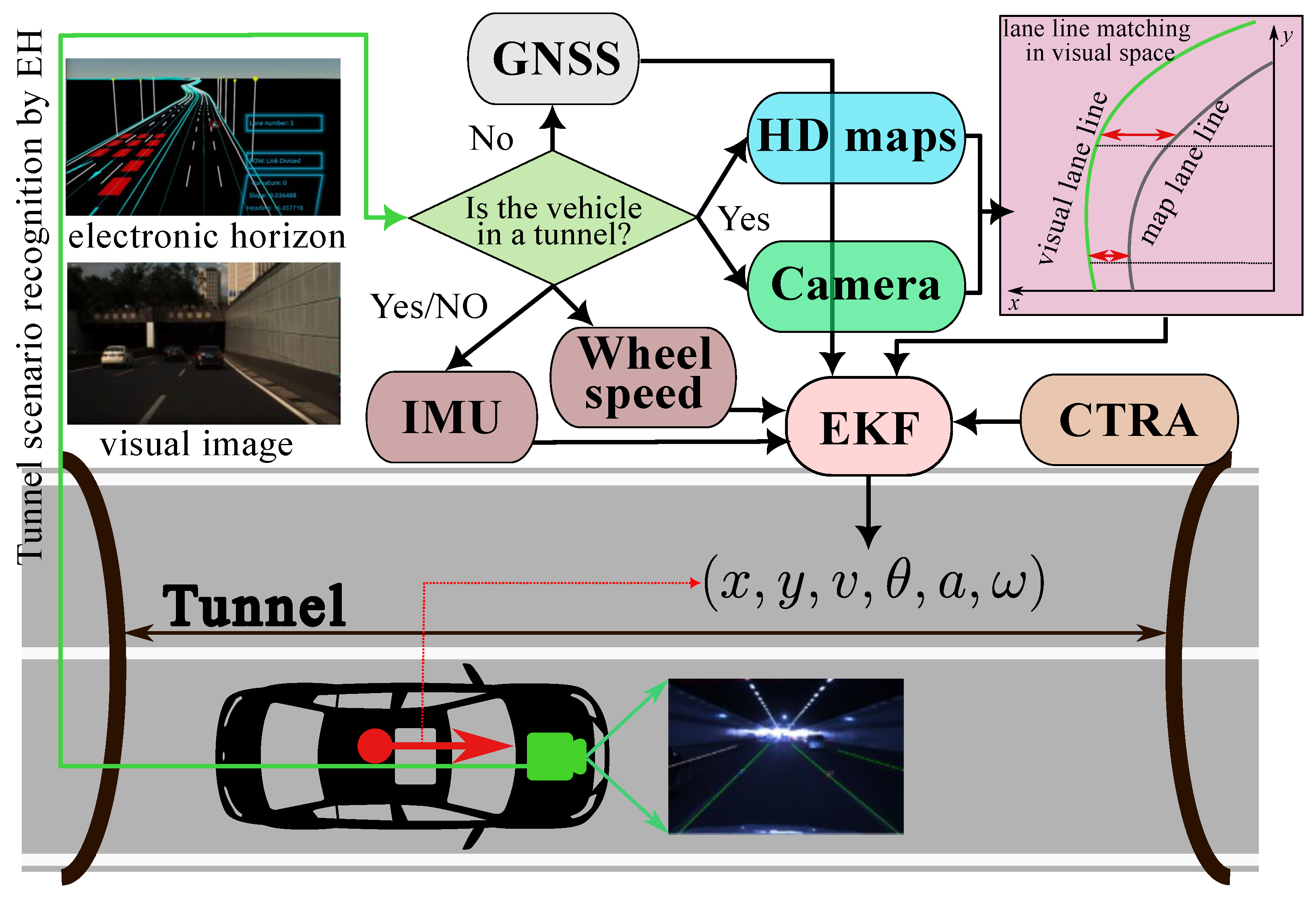
The EH greatly reduces the amount of topology network data that need to be transmitted to applications, making the HD map applications more efficient. Various properties obtained from the HD maps can therefore be provided to indicate a vehicle’s surrounding environment along its driving route, including road types such as bridges and tunnels as well as the starting and ending positions of these tunnels. By using these pieces of information along with vehicular data, such as position and speed, it is possible to accurately identify the current road scene and predict the upcoming road scenarios.

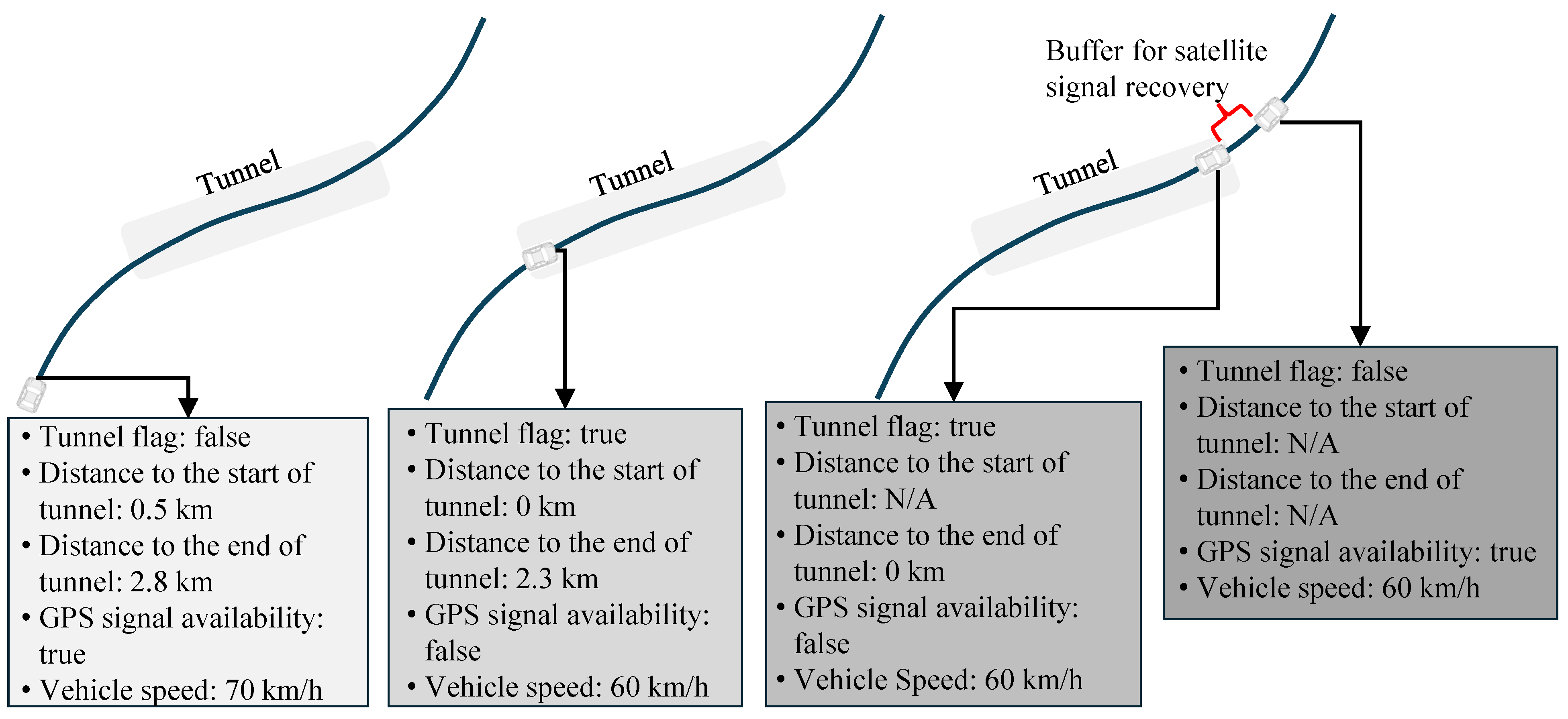
Specifically, using the EH and the current vehicle position, the distance to the upcoming tunnel can be determined, and the arrival time at the tunnel can be easily calculated. Figure 4 illustrates the patterns of the tunnel scenario identification process as a vehicle drives through a tunnel.

4.2. Lane Line Recognition Based on Deep Learning Method

The iBiSeNet proposed in this paper is depicted in Figure 5. This deep learning network is adopted for lane line recognition. The original BiSeNet [36], developed by Megvii Technology, is a real-time semantic segmentation network. Using ResNet-18 as a base model, the fast version of BiSeNet achieved 74.7% mean IOU (Intersection over Union) with the CitiScapes verification datasets at 65.5 FPS [36].

In this paper, we introduce two main modifications [43] to the original BiSeNet:

• We incorporate both local attention and multi-scale attention mechanisms, in contrast to the original BiSeNet, which uses only classic attention.
• We restore images by 4 times, 4 times, and 8 times deconvolution in the last three output steps, whereas the original BiSeNet employs 8 times, 8 times, and 16 times upsampling in its last three output layers.

After these modifications, the IOU of our BiSeNet is improved to 89.69% for the white lane line recognition, as shown in

Table 1. Performance of lane line recognition using iBiSeNet.

Method	Recall	Pixel Accuracy	IOU	Speed
Ours	92.42%	96.81%	89.69%	31 FPS
BiSeNet	–	–	74.70%	65.5 FPS

. Although the speed drops to 31 FPS, it still meets the real-time requirements in our application.

When the lane lines are recognized by the iBiSeNet, they are represented through cubic polynomials. To determine the optimal parameters of the recognized lane lines, a weighted least squares (WLS) algorithm [44] is employed to find the best-fitting parameters $c_0$, $c_1$, $c_2$, and $c_3$ for the cubic polynomial expressed by Equation (1), where $(x,y)$ denote the pixel coordinates in the image coordinate system.

$$y=c_3{x}^3+c_2{x}^2+c_{1}x+c_0$$

(1)

As shown in Figure 6, the iBiSeNet model effectively recognizes lane lines even in tunnel scenarios. The results of the cubic polynomial fitting are overlaid on the images, demonstrating the model’s accuracy in identifying and modeling the lane geometries.

4.3. Matching between Visual Lane Lines and HD Map Lane Lines

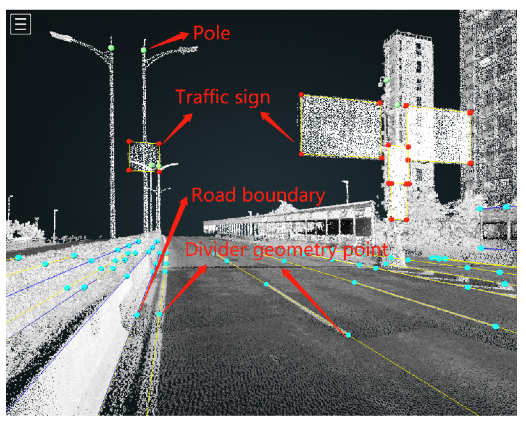
Since HD maps are pre-collected and produced, they can achieve a high spatial resolution of up to 20 cm. This accuracy is verified by using RTK control points and high-performance LiDAR point cloud data, as shown in Figure 7.

In order to match HD map lane lines with the visual lane lines recognized by our smart camera, it is essential to transform them into the same coordinate system. In this paper, the HD map lane lines are transformed into the image coordinate system of the on-board camera. This projection involves several transformations between different coordinate systems. The detailed process is described as follows.

As the HD maps are represented in a world coordinate system, firstly, we need to transform the world coordinates ${[x_w,y_w,z_w]}^T$ into camera body coordinates ${[x_c,y_c,z_c]}^T$ through a rigid transformation using a rotation matrix $\mathbf{R}$ and a translation vector $\mathbf{t}$:

$$\left[\begin{array}{c}{x}_c\\ y_c\\ z_c\end{array}\right]=\mathbf{R}\left[\begin{array}{c}{x}_w\\ y_w\\ z_w\end{array}\right]+\mathbf{t}$$

(2)

This equation can be further written in a homogeneous coordinate form:

$$\left[\begin{array}{c}{x}_c\\ y_c\\ z_c\\ 1\end{array}\right]={\mathbf{K}}_e\left[\begin{array}{c}{x}_w\\ y_w\\ z_w\\ 1\end{array}\right],{\mathbf{K}}_e=\left[\begin{array}{cc}\mathbf{R}& \mathbf{t}\\ {\mathbf{0}}_{1\times 3}& 1\end{array}\right]$$

(3)

where ${\mathbf{K}}_e$ is called the extrinsics of the camera, which are calibrated using the classical vanishing method [45], in this paper.

Then, the camera body coordinates are transformed into to image coordinates through:

$$z_c\left[\begin{array}{c}{x}_i\\ y_i\\ 1\end{array}\right]=\left[\begin{array}{cccc}f& 0& 0& 0\\ 0& f& 0& 0\\ 0& 0& 1& 0\end{array}\right]\left[\begin{array}{c}{x}_c\\ y_c\\ z_c\\ 1\end{array}\right]$$

(4)

where f is the focal length of the camera.

The image coordinates are further transformed into pixel coordinates via:

$$\left[\begin{array}{c}x\\ y\\ 1\end{array}\right]=\left[\begin{array}{ccc}\frac{1}{dx}& 0& x_0\\ 0& \frac{1}{dy}& y_0\\ 0& 0& 1\end{array}\right]\left[\begin{array}{c}{x}_i\\ y_i\\ 1\end{array}\right]$$

(5)

where $dx$ and $dy$ are the pixel length in the x and y direction, and $(x_0,y_0)$ is the principal point.

In summary, the transformation from the world coordinates ${[x_w,y_w,z_w]}^T$ to pixel coordinates ${[x,y]}^T$ is achieved through:

$$z_c\left[\begin{array}{c}x\\ y\\ 1\end{array}\right]={\mathbf{K}}_i{\mathbf{K}}_e\left[\begin{array}{c}{x}_w\\ y_w\\ z_w\\ 1\end{array}\right]$$

(6)

where

$${\mathbf{K}}_i=\left[\begin{array}{ccc}\frac{1}{dx}& 0& x_0\\ 0& \frac{1}{dy}& y_0\\ 0& 0& 1\end{array}\right]\left[\begin{array}{cccc}f& 0& 0& 0\\ 0& f& 0& 0\\ 0& 0& 1& 0\end{array}\right]$$

(7)

and ${\mathbf{K}}_i$ is called the intrinsics of the camera.

Once the HD map lane lines are projected to the pixel coordinate system, three deviation variables—vertical deviation $\delta x$, horizontal deviation $\delta y$, and yaw deviation $\delta \theta$—are applied to match the lane lines of HD maps with those recognized by the camera. The matching process, illustrated in Figure 8, is a typical nonlinear optimization problem. We seek the optimal vector, as expressed in Equation (8), to minimize the differences between the projected HD map lane lines and the visually recognized lane lines at specified positions $i=0,\cdots ,n$.

$$\mathbf{d}=\left[\begin{array}{c}\delta x\\ \delta y\\ \delta \theta \end{array}\right]$$

(8)

Therefore, the following object function is designed:

$$f\left(x\right)=\underset{\mathbf{d}=[\delta x,\delta y,\delta \theta ]}{min}\frac{{\displaystyle \sum _0^n}{\parallel y_i^{map}-y\left(x_i\right)\parallel }^2}{2}$$

(9)

where $y_i^{map}$ is the y coordinate data of map lane lines in visual space at position $x_i$, and $y\left(x_i\right)$ is the cubic polynomial function of a visual lane line that is recognized by the on-board camera.

We employ the Levenberg–Marquardt (LM) method [46] to solve this object function, using feature points at $i=\{0,10\}$ in this paper.

In order to match the visual lane line with the HD map lane line, we firstly calculate the deviated positions via applying the deviation vector $\mathbf{d}={[\delta x,\delta y,\delta \theta ]}^T$ to the visual lane line that is described by Equation (1):

$$y\left(x\right)=c_3{(x-\delta x)}^3+c_2{(x-\delta x)}^2+tan(\delta \theta +arctan\left(c_1\right))(x-\delta x)+(c_0+\delta y)$$

(10)

At feature position $x_i$, the residual distance $r_i$ between the map lane line and the visual lane line can be calculated through:

$$r_i=y_i^{map}-y\left(x_i\right)$$

(11)

Substituting $x=0$ into Equation (10), we can calculate the residual distance at the first feature point:

$$r_0\left(\mathbf{d}\right)=y_0^{map}+[c_3{\left(\delta x\right)}^3-c_2{\left(\delta x\right)}^2+tan(\delta \theta +arctan\left(c_1\right))\left(\delta x\right)-(c_0+\delta y)]$$

(12)

and for $x=10$, the residual distance at the second feature point is calculated through:

$$r_{10}\left(\mathbf{d}\right)=y_{10}^{map}-[c_3{(10-\delta x)}^3+c_2{(10-\delta x)}^2+tan(\delta \theta +arctan\left(c_1\right))(10-\delta x)-(c_0+\delta y)]$$

(13)

These two residual distances $r_0$ and $r_{10}$, functions of the deviation vector $\mathbf{d}$, are used to feature the distance between the visual lane line and HD map lane line. To minimize the sum of these residual distances, matching these lane lines, the following object function is constructed:

$$\left[\begin{array}{c}{r}_0\\ r_{10}\end{array}\right]=f\left(\mathbf{d}\right)=\left[\begin{array}{c}{r}_0\left(\mathbf{d}\right)\\ r_{10}\left(\mathbf{d}\right)\end{array}\right]$$

(14)

This function can be solved through the LM algorithm. Firstly, the Jacobian of Equation (14) is calculated through:

$$\mathbf{J}\left(\mathbf{d}\right)=\frac{\partial f\left(\mathbf{d}\right)}{\partial \mathbf{d}}=\left[\begin{array}{ccc}\frac{\partial r_0}{\delta x}& \frac{\partial r_0}{\delta y}& \frac{\partial r_0}{\delta \theta }\\ \frac{\partial r_{10}}{\partial \delta x}& \frac{\partial r_{10}}{\partial \delta y}& \frac{\partial r_{10}}{\partial \delta \theta }\end{array}\right]$$

(15)

where

$$\begin{array}{cc}\hfill & \frac{\partial r_0}{\partial \delta x}=3c_3\delta x^2-2c_2\delta x+tan(\delta \theta +arctan\left(c_1\right))\hfill \\ \hfill & \frac{\partial r_{10}}{\partial \delta x}=3c_3{(10-\delta x)}^2+2c_2(10-\delta x)+tan(\delta \theta +arctan\left(c_1\right))\hfill \\ \hfill & \frac{\partial r_0}{\partial \delta y}=-1\hfill \\ \hfill & \frac{\partial r_{10}}{\partial \delta y}=-1\hfill \\ \hfill & \frac{\partial r_0}{\partial \delta \theta }=\frac{\delta x}{\cos {(\delta \theta +arctan\left(c_1\right))}^2}\hfill \\ \hfill & \frac{\partial r_{10}}{\partial \delta \theta }=\frac{\delta x-10}{\cos {(\delta \theta +arctan\left(c_1\right))}^2}\hfill \end{array}$$

(16)

Then, according to the LM algorithm, the optimal $\mathbf{d}$ can be found using the following iteration equation:

$${\mathbf{d}}_{i+1}={\mathbf{d}}_i-{[{\mathbf{J}}^T\left({\mathbf{d}}_i\right)\mathbf{J}\left({\mathbf{d}}_i\right)+\lambda \mathrm{diag}\left({\mathbf{J}}^T\left({\mathbf{d}}_i\right)\mathbf{J}\left({\mathbf{d}}_i\right)\right)]}^{-1}{\mathbf{J}}^T\left({\mathbf{d}}_i\right)f\left({\mathbf{d}}_i\right)$$

(17)

where $\lambda$ is the damping parameter.

As the visual lane line and HD map lane line are matched, consequently, we are able to acquire accurate geometry data from HD maps to correct our vehicle pose even when GNSS data are unavailable.

4.4. Multi-Source Information Fusion for Vehicular Localization Using EKF

The EKF and unscented KF (UKF) are standard solutions for nonlinear state estimation. In EKF, the nonlinearities are approximated analytically through first-order Taylor expansion. In contrast, UKF uses a set of deterministically sampled sigma points to capture the true mean and covariance of the Gaussian random variables and, when propagated through the true nonlinearity, captures the posterior mean and covariance accurate to the third order (Taylor expansion) for any nonlinearity. This feature allows UKF to achieve accurate estimations in highly nonlinear and dynamic motion scenarios [47].

However, in vehicle state estimation, the vehicle’s motion is approximately linear in a short time interval. Our previous study [48] shows that the accuracy performance of EKF and UKF is close, whereas EKF demonstrates higher speed than UKF. Even in more complex vehicle motion prediction tasks [49], EKF is primarily used. To ensure the system’s high efficiency, an EKF that cooperates with a constant turn rate and acceleration (CTRA) model is employed in this paper. The system state is:

$${\mathbf{x}}_k=\left[\begin{array}{c}{x}_k\\ y_k\\ v_k\\ {\theta }_k\\ a_k\\ {\omega }_k\end{array}\right]$$

(18)

where $(x_k,y_k)$ is the position coordinates, ${\theta }_k$ the yaw angle, $v_k$ the velocity, $a_k$ the acceleration, and ${\omega }_k$ the yaw rate at instant k. The system is described by the CTRA model as follows:

$${\mathbf{x}}_{k+1}^{-}=f_{CTRA}\left({\mathbf{x}}_k^{+}\right)={\mathbf{x}}_k^{+}+\left[\begin{array}{c}\Delta x\\ \Delta y\\ a_k\Delta t\\ {\omega }_k\Delta t\\ 0\\ 0\end{array}\right]$$

(19)

where

$$\Delta x=\frac{\left[(v_k+a_k\Delta t)\sin ({\theta }_k+{\omega }_k\Delta t)-v_k\sin \left({\theta }_k\right)\right]}{{\omega }_k}+\frac{a_k\left[\cos ({\theta }_k+{\omega }_k\Delta t)-\cos \left({\theta }_k\right)\right]}{{\omega }_k^2}$$

(20)

and

$$\Delta y=\frac{\left[-(v_k+a_k\Delta t)\cos ({\theta }_k+{\omega }_k\Delta t)+v_k\cos \left({\theta }_k\right)\right]}{{\omega }_k}+\frac{a_k\left[\sin ({\theta }_k+{\omega }_k\Delta t)-\sin \left({\theta }_k\right)\right]}{{\omega }_k^2}$$

(21)

In our EKF, the vehicle state prediction is performed by the above CTRA model:

$${\mathbf{x}}_{k+1}^{-}=f_{CTRA}\left({\mathbf{x}}_k^{+}\right)$$

(22)

and the covariance is predicted through:

$${\mathbf{P}}_{k+1}^{-}={\mathbf{J}}_{f_{CTRA}}\left({\mathbf{x}}_k^{+}\right){\mathbf{P}}_k^{+}{\mathbf{J}}_{f_{CTRA}}^T\left({\mathbf{x}}_k^{+}\right)+{\mathbf{Q}}_k$$

(23)

where ${\mathbf{Q}}_k$ is the known system covariance matrix, and ${\mathbf{J}}_{f_{CTRA}}(·)$ is the Jacobain of the CTRA model.

As soon as the on-board sensor/visual matching measurements are available, the EKF’s prediction is corrected through:

$${\mathbf{x}}_{k+1}^{+}={\mathbf{x}}_{k+1}^{-}+{\mathbf{K}}_{k+1}({\mathbf{y}}_{k+1}-h\left({\mathbf{x}}_{k+1}^{-}\right))$$

(24)

where $h(·)$ is the measurement function and ${\mathbf{K}}_k$ is the Kalman gain matrix, which is as follows:

$${\mathbf{K}}_{k+1}={\mathbf{P}}_{k+1}^{-}{\mathbf{J}}_h^T\left({\mathbf{x}}_{k+1}^{-}\right){[{\mathbf{J}}_h\left({\mathbf{x}}_{k+1}^{-}\right){\mathbf{P}}_{k+1}^{-}{\mathbf{J}}_h^T\left({\mathbf{x}}_{k+1}^{-}\right)+{\mathbf{R}}_{k+1}]}^{-1}$$

(25)

where $\mathbf{R}$ is the measurement covariance, and ${\mathbf{J}}_h(·)$ is the Jacobian function of measurement model $h(·)$. In this paper, ${\mathbf{J}}_h(·)=\mathbf{I}$, due to the following measurement models that are applied in different scenarios being linear:

• If a vehicle is outside a tunnel, the position measurements are directly derived from the GNSS at 10 Hz:

  $$\begin{array}{cc}\hfill & x_k=x_k^{gnss}\hfill \\ \hfill & y_k=y_k^{gnss}\hfill \end{array}$$

  (26)
• If the vehicle is driving in a tunnel, where the GNSS signals are unavailable, the vehicle’s pose measurements are obtained through vision-and-HD-map matching at 30 Hz:

  $$\begin{array}{cc}\hfill & x_k=x_k^{match}\hfill \\ \hfill & y_k=y_k^{match}\hfill \\ \hfill & {\theta }_k={\theta }_k^{match}\hfill \end{array}$$

  (27)
• The IMU and wheel speed measurements, which remain obtainable, are directly used to update the vehicle’s acceleration, yaw rate, and velocity at 100 Hz:

  $$\begin{array}{cc}\hfill & a_k=a_k^{imu}\hfill \\ \hfill & {\omega }_k={\omega }_k^{imu}\hfill \\ \hfill & v_k=v_k^{wheel}\hfill \end{array}$$

  (28)

Finally, the covariance matrix is updated through:

$${\mathbf{P}}_{k+1}^{+}=[\mathbf{I}-{\mathbf{K}}_{k+1}{\mathbf{J}}_h\left({\mathbf{x}}_{k+1}^{-}\right)]{\mathbf{P}}_{k+1}^{-}$$

(29)

The details of the EKF’s implementation, including initialization, parameter configurations, Jacobains, and time synchronization, can be found in [48].

5. Experiments

5.1. Experimental Configurations

Our experiments were carried out on public roads in Nanjing City. The experimental field is shown in Figure 9.

The entire experimental route is about 36 km in total, with nine consecutive tunnels, JiQingMen Tunnel, ShuiXiMen Tunnel, QingLiangMen Tunnel, CaoChangMen Tunnel, MoFanMaLu Tunnel, XuanWuHu Tunnel, JiuHuaShan Tunnel, XiAnMen Tunnel, and TongJiMen Tunnel, with a total length of 12.86 km accounting for 35% of length of the entire route, as presented in

Table 2. Information of tunnels in the experimental route.

Tunnel	JiQingMen	ShuiXiMen	QingLiangMen	CaoChangMen	MoFanMaLu
Tunnel Length	0.59 km	0.56 km	0.87 km	0.74 km	1.45 km
Tunnel	XuanWuHu	JiuHuaShan	XiAnMen	TongJiMen	Total tunnel length
Tunnel Length	2.66 km	2.78 km	1.77 km	1.44 km	12.86 km
Route length	36.38 km				12.86/36.38 = 35%

.

All the sensors used in our experiments are affordable for consumers. A low-cost integrated navigation system, Npos320 (https://daobook.github.io/apollo-doc-old/docs/specs/Navigation/Npos320_guide.html (accessed on 15 May 2024)), is used as the GNSS and IMU module, and a normal web camera is used in the camera module. To obtain ground truth data to assess the localization performance of our system, a high-end GNSS and IMU product called IMU-ISA-100C (https://novatel.com/products/gnss-inertial-navigation-systems/imus/isa-100c (accessed on 15 May 2024)) is employed. With post-difference processing, it could be ensured that the errors of the ground truth data are less than 5 cm. The installation of these sensors is demonstrated in Figure 10.

The rotation matrices and translation vectors that are used to transform the local measurements of the camera, GNSS, IMU, and other sensors to a unified positioning coordinate system are determined by external parameter calibrations.

5.2. Error Evaluation

The localization errors’ space distribution is shown in Figure 11. The left and right halves represent the lateral and longitudinal errors, respectively. Different colors are used to indicate the accuracy of positioning at the sampled track points. For brevity, the original experimental results are down-sampled using a ratio of 10:1.

This figure clearly shows that the lateral positioning error is within 0.3 m, and most of the longitudinal positioning errors are less than 3 m within the entire trip driving through the nine continuous tunnels. During the initial phases, as the vehicle enters XuanWuHu and JiuHuaShan tunnels, there are brief periods where longitudinal errors exceed 6 m, as evidenced by two distinct red point segments on the right side of Figure 11. This occurrence can be attributed to the fact that these two tunnels are situated beneath the XuanWu lake and are deeper than the others. The large longitudinal errors result from the abrupt changes in elevation. Since our kinematic model is two-dimensional, lacking representation in the z axis, it therefore performs poorly in such tunnel spaces. Fortunately, these deviations are promptly corrected by GNSS measurements upon the vehicle’s exit from the tunnels, thanks to the EH module’s clever switching of sensor measurements for different scenarios.

There are several potential solutions to address this problem: (1) employing a three-dimensional vehicle motion model in the EKF; (2) using additional landmarks, such as arrows, to refine the longitudinal estimates. These strategies remain areas for future investigation in our work.

The time-series localization errors are presented in Figure 12. The figure demonstrates that our system maintains accurate lateral localization throughout the entire experiment, correctly identifying the current driving lane. For longitudinal localization errors, several peaks are observed during the experiment, primarily due to GNSS-denied environments, such as tunnels and overpasses. However, as soon as GNSS signals become available, the longitudinal errors are corrected immediately.

The mean absolute error (MAE) and standard deviation (StD) metrics in Equation (30) are used to quantify the localization performance.

$$MAE=\frac{1}{N}\sum _{i=1}^N|x_i-x_i^{true}|,StD=\sqrt{\frac{1}{N}\sum _{i=1}^N{(x_i-\overline{x})}^2}$$

(30)

where $x_i$ is the value of an estimate and $x_i^{true}$ is corresponding true value; $\overline{x}$ represents the mean value of $x_i$.

The overall quantitative and comparative results are summarized in

Table 3. MAE and StD of GNSS/IMU/Camera/HD Map integrated localization.

Item	Lateral Error (m)	Longitudinal Error (m)	Yaw Error (Degree)
MAE	0.041	0.701	0.899
StD	0.086	1.827	0.669

and

Table 4. MAE within different percentiles (GNSS/IMU/Camera/HD Map integrated localization).

Percentile	Lateral MAE (m)	Longitudinal MAE (m)	Yaw MAE (Degree)
50%	0.051	0.454	0.890
75%	0.078	1.452	1.028
80%	0.087	2.039	1.072
85%	0.103	2.671	1.132
90%	0.138	3.251	1.233
95%	0.203	4.869	1.474
99%	0.299	7.111	3.758

for our GNSS/IMU/Camera/HD Map integrated localization system and

Table 5. MAE and StD of GNSS/IMU integrated localization.

Item	Lateral Error (m)	Longitudinal Error (m)	Yaw Error (Degree)
MAE	4.638	16.546	2.960
StD	20.851	59.208	0.575

and

Table 6. MAE within different percentiles (GNSS/IMU integrated localization).

Percentile	Lateral MAE (m)	Longitudinal MAE (m)	Yaw MAE (Degree)
50%	0.152	1.227	2.882
75%	3.845	33.454	3.273
80%	6.466	51.796	3.378
85%	10.806	70.849	3.486
90%	19.039	98.656	3.660
95%	45.293	152.676	4.207
99%	126.262	231.995	4.774

for a comparison with a GNSS/IMU integrated localization system.

For our system, the mean lateral localization error is 0.041 m, with a StD of 0.701 m. According to Table 4, 99% of the positioning errors are less than 0.299 m laterally and 7.111 m longitudinally. The experimental results demonstrate that our system achieves high accuracy in lateral localization. The StD of 0.701 m and the MAE value of 0.299 m for 99% of lateral errors indicate that correct lane identification can always be maintained using our system. In the longitudinal direction, the MAE is 0.701 m with a StD of 1.827 m, which is generally satisfactory in most cases. However, some exceptionally large errors occur in longitudinal localization, indicating a need for further optimization.

To demonstrate the advantages of the localization method proposed in this paper, particularly the performance of vision and HD map matching, we conducted additional comparative experiments using only a GNSS and an IMU. The results are shown in Table 5 and Table 6. The lateral MAE is 4.638 m, and the longitudinal MAE is 16.546 m, which are significantly greater than those of our system, demonstrating our superiority. According to Table 6, only 50% of lateral localization errors are less than 0.152 m, indicating that correct lane identification cannot be guaranteed most of the time. The 99th percentile MAE is 126.262 m laterally and 231.995 m error longitudinally, showing that GNSS and IMU integration is insufficient for handling challenging continuous tunnel scenarios.

6. Conclusions

In this paper, we propose a GNSS/IMU/camera/HD map fusion localization solution for AVs. In this system, an improved real-time semantic segmentation model based on BiSeNet is used to extract the lane lines from the images captured by the camera in real time; then, these lane lines are modeled through cubic polynomials and matched with the lane lines acquired from the HD map using electronic horizon technologies. The pose correction is obtained by the optimal matching using the LM algorithm. Finally, utilizing the CTRA motion model and an EKF, the multi-source information from the GNSS, IMU, camera, wheel odometry, and HD maps are fused to achieve high-performance localization in challenging urban tunnel scenarios. The experimental results show that our system achieves lane-level localization accuracy, with a lateral error of less than 0.29 m in continuous tunnel scenarios most of the time, and the average accuracy in the longitudinal direction is 0.70 m.

In the future, matching between other visually recognized targets such as ground text, arrows, symbols, traffic signs, traffic lights, and HD maps will be explored to improve the accuracy in longitudinal direction. The positioning, navigation, and timing (PNT) information provided by “5G + BDS/GNSS” will be explored as lower latency can effectively improve positioning accuracy [50]. Additionally, further comparisons with other related studies will be conducted.

References

1. Groves, P.D. Principles of gnss, inertial, and multisensor integrated navigation systems, [book review]. IEEE Aerosp. Electron. Mag. 2015, 30, 26–27. [Google Scholar] [CrossRef]
2. Jackson, J.; Davis, B.; Gebre-Egziabher, D. A performance assessment of low-cost rtk gnss receivers. In Proceedings of the 2018 IEEE/ION Position, Location and Navigation Symposium (PLANS), Monterey, CA, USA, 23–26 April 2018; pp. 642–649. [Google Scholar]
3. Binder, Y.I. Dead reckoning using an attitude and heading reference system based on a free gyro with equatorial orientation. Gyroscopy And Navig. 2017, 8, 104–114. [Google Scholar] [CrossRef]
4. Noureldin, A.; Karamat, T.B.; Georgy, J. Fundamentals of Inertial Navigation, Satellite-Based Positioning and Their Integration; Springer Science & Business Media: New York, NY, USA, 2012. [Google Scholar]
5. Zaminpardaz, S.; Teunissen, P.J. Analysis of galileo iov+ foc signals and e5 rtk performance. GPS Solut. 2017, 21, 1855–1870. [Google Scholar] [CrossRef]
6. Qin, H.; Peng, Y.; Zhang, W. Vehicles on rfid: Error-cognitive vehicle localization in gps-less environments. IEEE Trans. Veh. 2017, 66, 9943–9957. [Google Scholar] [CrossRef]
7. Liu, Y.; Fan, X.; Lv, C.; Wu, J.; Li, L.; Ding, D. An innovative information fusion method with adaptive kalman filter for integrated ins/gps navigation of autonomous vehicles. Mech. Syst. Signal Process. 2018, 100, 605–616. [Google Scholar] [CrossRef]
8. Zhang, J.; Singh, S. Loam: Lidar odometry and mapping in real-time. In Robotics: Science and Systems; The MIT Press: Berkeley, CA, USA, 2014; Volume 2, pp. 1–9. [Google Scholar]
9. Joshi, A.; James, M.R. Generation of accurate lane-level maps from coarse prior maps and lidar. IEEE Intell. Transp. Syst. 2015, 7, 19–29. [Google Scholar] [CrossRef]
10. Chen, A.; Ramanandan, A.; Farrell, J.A. High-precision lane-level road map building for vehicle navigation. In Proceedings of the IEEE/ION Position, Location and Navigation Symposium, Indian Wells, CA, USA, 4–6 May 2010; pp. 1035–1042. [Google Scholar]
11. Nedevschi, S.; Popescu, V.; Danescu, R.; Marita, T.; Oniga, F. Accurate ego-vehicle global localization at intersections through alignment of visual data with digital map. IEEE Trans. Intell. Transp. Syst. 2012, 14, 673–687. [Google Scholar] [CrossRef]
12. Strijbosch, W. Safe autonomous driving with high-definition maps. ATZ Worldw. 2018, 120, 28–33. [Google Scholar] [CrossRef]
13. Varnhagen, R. Electronic Horizon: A Map as a Sensor and Predictive Control; SAE Technical Paper: Warrendale, PA, USA, 2017. [Google Scholar]
14. Horita, Y.; Schwartz, R.S. Extended electronic horizon for automated driving. In Proceedings of the 2015 14th International Conference on ITS Telecommunications (ITST), Copenhagen, Denmark, 2–4 December 2015; pp. 32–36. [Google Scholar]
15. Ress, C.; Etemad, A.; Kuck, D.; Requejo, J. Electronic horizon-providing digital map data for adas applications. In Proceedings of the 2nd International Workshop on Intelligent Vehicle Control Systems (IVCS), Madeira, Portugal, 11–15 May 2008; Volume 2008, pp. 40–49. [Google Scholar]
16. Ress, C.; Balzer, D.; Bracht, A.; Durekovic, S.; Löwenau, J. Adasis protocol for advanced in-vehicle applications. In Proceedings of the 15th World Congress on Intelligent Transport Systems, New York, NY, USA, 16–20 November 2008; Volume 7. [Google Scholar]
17. Durekovic, S.; Smith, N. Architectures of map-supported adas. In Proceedings of the 2011 IEEE Intelligent Vehicles Symposium (IV), Baden-Baden, Germany, 5–9 June 2011; pp. 207–211. [Google Scholar]
18. Wiesner, C.A.; Ruf, M.; Sirim, D.; Klinker, G. Visualisation of the electronic horizon in head-up-displays. In Proceedings of the 2016 IEEE International Symposium on Mixed and Augmented Reality (ISMAR-Adjunct), Merida, Mexico, 19–23 September 2016; pp. 87–89. [Google Scholar]
19. Gao, B.; Hu, G.; Zhu, X.; Zhong, Y. A robust cubature kalman filter with abnormal observations identification using the mahalanobis distance criterion for vehicular ins/gnss integration. Sensors 2019, 19, 5149. [Google Scholar] [CrossRef]
20. Gao, G.; Gao, B.; Gao, S.; Hu, G.; Zhong, Y. A hypothesis test-constrained robust kalman filter for ins/gnss integration with abnormal measurement. IEEE Trans. Veh. Technol. 2022, 72, 1662–1673. [Google Scholar] [CrossRef]
21. Gao, G.; Zhong, Y.; Gao, S.; Gao, B. Double-channel sequential probability ratio test for failure detection in multisensor integrated systems. IEEE Trans. Instrum. Meas. 2021, 70, 3514814. [Google Scholar] [CrossRef]
22. Cvišić, I.; Marković, I.; Petrović, I. Soft2: Stereo visual odometry for road vehicles based on a point-to-epipolar-line metric. IEEE Trans. Robot. 2022, 39, 273–288. [Google Scholar] [CrossRef]
23. Fraundorfer, F.; Scaramuzza, D. Visual odometry: Part i: The first 30 years and fundamentals. IEEE Robot. Autom. Mag. 2011, 18, 80–92. [Google Scholar]
24. Geiger, A.; Lenz, P.; Urtasun, R. Are we ready for autonomous driving? the kitti vision benchmark suite. In Proceedings of the 2012 IEEE Conference on Computer Vision and Pattern Recognition, Providence, RI, USA, 16–21 June 2012; pp. 3354–3361. [Google Scholar]
25. Geiger, A.; Lenz, P.; Stiller, C.; Urtasun, R. The Kitti Vision Benchmark Suite. Available online: http://www.cvlibs.net/datasets/kitti (accessed on 24 May 2024).
26. Schreiber, M.; Knöppel, C.; Franke, U. Laneloc: Lane marking based localization using highly accurate maps. In Proceedings of the 2013 IEEE Intelligent Vehicles Symposium (IV), Gold Coast, QLD, Australia, 23–26 June 2013; pp. 449–454. [Google Scholar]
27. Dickmanns, E.D.; Zapp, A. A curvature-based scheme for improving road vehicle guidance by computer vision. In Mobile Robots I; SPIE: Bellingham, WA, USA, 1987; Volume 727, pp. 161–168. [Google Scholar]
28. Gruyer, D.; Belaroussi, R.; Revilloud, M. Map-aided localization with lateral perception. In Proceedings of the 2014 IEEE Intelligent Vehicles Symposium Proceedings, Dearborn, MI, USA, 8–11 June 2014; pp. 674–680. [Google Scholar]
29. Xiao, Z.; Yang, D.; Wen, F.; Jiang, K. A unified multiple-target positioning framework for intelligent connected vehicles. Sensors 2019, 19, 1967. [Google Scholar] [CrossRef] [PubMed]
30. Cui, D.; Xue, J.; Zheng, N. Real-time global localization of robotic cars in lane level via lane marking detection and shape registration. IEEE Trans. Intell. Transp. Syst. 2015, 17, 1039–1050. [Google Scholar] [CrossRef]
31. Xiao, Z.; Yang, D.; Wen, T.; Jiang, K.; Yan, R. Monocular localization with vector hd map (mlvhm): A low-cost method for commercial ivs. Sensors 2020, 20, 1870. [Google Scholar] [CrossRef] [PubMed]
32. Wang, H.; Xue, C.; Zhou, Y.; Wen, F.; Zhang, H. Visual semantic localization based on hd map for autonomous vehicles in urban scenarios. In Proceedings of the 2021 IEEE International Conference on Robotics and Automation (ICRA), Xi’an, China, 30 May–5 June 2021; pp. 11255–11261. [Google Scholar]
33. Wen, T.; Xiao, Z.; Wijaya, B.; Jiang, K.; Yang, M.; Yang, D. High precision vehicle localization based on tightly-coupled visual odometry and vector hd map. In Proceedings of the 2020 IEEE Intelligent Vehicles Symposium (IV), Las Vegas, NV, USA, 19 October–13 November 2020; pp. 672–679. [Google Scholar]
34. Guo, C.; Lin, M.; Guo, H.; Liang, P.; Cheng, E. Coarse-to-fine semantic localization with hd map for autonomous driving in structural scenes. In Proceedings of the 2021 IEEE/RSJ International Conference on Intelligent Robots and Systems (IROS), Prague, Czech Republic, 27 September–1 October 2021; pp. 1146–1153. [Google Scholar]
35. Wen, T.; Jiang, K.; Wijaya, B.; Li, H.; Yang, M.; Yang, D. Tm 3 loc: Tightly-coupled monocular map matching for high precision vehicle localization. IEEE Trans. Intell. Transp. 2022, 23, 20268–20281. [Google Scholar] [CrossRef]
36. Yu, C.; Wang, J.; Peng, C.; Gao, C.; Yu, G.; Sang, N. Bisenet: Bilateral segmentation network for real-time semantic segmentation. In Proceedings of the European Conference on Computer Vision (ECCV), Munich, Germany, 8–14 September 2018; pp. 325–341. [Google Scholar]
37. Yu, C.; Gao, C.; Wang, J.; Yu, G.; Shen, C.; Sang, N. Bisenet v2: Bilateral network with guided aggregation for real-time semantic segmentation. Int. J. Comput. Vis. 2021, 129, 3051–3068. [Google Scholar] [CrossRef]
38. Wan, G.; Yang, X.; Cai, R.; Li, H.; Zhou, Y.; Wang, H.; Song, S. Robust and precise vehicle localization based on multi-sensor fusion in diverse city scenes. In Proceedings of the 2018 IEEE International Conference on Robotics and Automation (ICRA), Brisbane, QLD, Australia, 21–25 May 2018; pp. 4670–4677. [Google Scholar]
39. Wu, C.-H.; Su, W.-H.; Ho, Y.-W. A study on gps gdop approximation using support-vector machines. IEEE Trans. Instrum. Meas. 2010, 60, 137–145. [Google Scholar] [CrossRef]
40. Aboutaleb, A.; El-Wakeel, A.S.; Elghamrawy, H.; Noureldin, A. Lidar/riss/gnss dynamic integration for land vehicle robust positioning in challenging gnss environments. Remote Sens. 2020, 12, 2323. [Google Scholar] [CrossRef]
41. Skog, I.; Handel, P. In-car positioning and navigation technologies-a survey. IEEE Trans. Intell. Transp. Syst. 2009, 10, 4–21. [Google Scholar] [CrossRef]
42. Lecce, V.D.; Amato, A. Route planning and user interface for an advanced intelligent transport system. IET Intell. Transp. Syst. 2011, 5, 149–158. [Google Scholar] [CrossRef]
43. Zhang, P.; Zhang, M.; Liu, J. Real-time hd map change detection for crowdsourcing update based on mid-to-high-end sensors. Sensors 2021, 21, 2477. [Google Scholar] [CrossRef] [PubMed]
44. Jung, S.; Youn, J.; Sull, S. Efficient lane detection based on spatiotemporal images. IEEE Trans. Intell. Transp. Syst. 2015, 17, 289–295. [Google Scholar] [CrossRef]
45. Caprile, B.; Torre, V. Using vanishing points for camera calibration. Int. J. Comput. Vis. 1990, 4, 127–139. [Google Scholar] [CrossRef]
46. Moré, J.J. The levenberg-marquardt algorithm: Implementation and theory. In Numerical Analysis: Proceedings of the Biennial Conference, Dundee, UK, 28 June–1 July 1977; Springer: Cham, Switzerland, 2006; pp. 105–116. [Google Scholar]
47. Hu, G.; Xu, L.; Gao, B.; Chang, L.; Zhong, Y. Robust unscented kalman filter based decentralized multi-sensor information fusion for ins/gnss/cns integration in hypersonic vehicle navigation. IEEE Trans. Instrum. Meas. 2023, 72, 8504011. [Google Scholar] [CrossRef]
48. Tao, L.; Watanabe, Y.; Yamada, S.; Takada, H. Comparative evaluation of kalman filters and motion models in vehicular state estimation and path prediction. J. Navig. 2021, 74, 1142–1160. [Google Scholar] [CrossRef]
49. Tao, L.; Watanabe, Y.; Takada, H. Geo-spatial and temporal relation driven vehicle motion prediction: A geographic perspective. IEEE Trans. Intell. Veh. 2024. early access. [Google Scholar] [CrossRef]
50. Liu, J.; Gao, K.; Guo, W.; Cui, J.; Guo, C. Role, path, and vision of “5g+ bds/gnss”. Satell. Navig. 2020, 1, 23. [Google Scholar] [CrossRef]
Figure 1. The proposed GNSS/IMU/Camera/HD map integrated localization system.
Remotesensing 16 02230 g001
Figure 2. System overview; the key technologies used in this system are highlighted in blue text.
Remotesensing 16 02230 g002
Figure 3. A demonstration of the EH (electronic horizon) applied in this paper. The left column: real world; the right column: electronic horizon. In the top-right of the figure, the EH provides the following pieces of information: Lane Number: 3 (the vehicle is in the third lane (from the left) of the road); FOW (form of way): Link Divided (the road ahead is divided); Curvature: 0; Slope: 0.036488%; Heading: 16.457718 degrees. In the bottom-right of the figure, the EH provides the following pieces of information: Tunnel (the vehicle is in a tunnel); Lane Number: 3; FOW: Link Divided; Curvature: 0; Slope: 0.041921%; Heading: 16.787982 degrees.
Remotesensing 16 02230 g003
Figure 4. Explanations of tunnel scenario identification patterns using an EH.
Remotesensing 16 02230 g004
Figure 5. The iBiSeNet for lane line recognition.
Remotesensing 16 02230 g005
Figure 6. Snapshots of lane line recognition and cubic polynomial fitting in tunnel scenarios.
Remotesensing 16 02230 g006
Figure 7. Accuracy verification of HD maps.
Remotesensing 16 02230 g007
Figure 8. Matching between the visual lane line and HD map lane line.
Remotesensing 16 02230 g008
Figure 9. Experimental field and tunnel scenes in Nanjing City (image: Google).
Remotesensing 16 02230 g009
Figure 10. Experimental vehicle and sensors.
Remotesensing 16 02230 g010
Figure 11. Localization errors’ space distribution; these points are down-sampled using a 10:1 ratio; the left: lateral errors; the right: longitudinal errors; unit: meter.
Remotesensing 16 02230 g011
Figure 12. The time-series error data in lateral and longitudinal localization; the left: lateral error (positive: right shift; negative: left shift); the right: longitudinal error (positive: forward shift; negative: backward shift).
Remotesensing 16 02230 g012