A New Retrieval Algorithm of Fractional Snow over the Tibetan Plateau Derived from AVH09C1

Abstract

Snow cover products are primarily derived from the Moderate-resolution Imaging Spectrometer (MODIS) and Advanced Very-High-Resolution Radiometer (AVHRR) datasets. MODIS achieves both snow/non-snow discrimination and snow cover fractional retrieval, while early AVHRR-based snow cover products only focused on snow/non-snow discrimination. The AVHRR Climate Data Record (AVHRR-CDR) provides a nearly 40-year global dataset that has the potential to fill the gap in long-term snow cover fractional monitoring. Our study selects the Qinghai–Tibet Plateau as the experimental area, utilizing AVHRR-CDR surface reflectance data (AVH09C1) and calibrating with the MODIS snow product MOD10A1. The snow cover percentage retrieval from the AVHRR dataset is performed using Surface Reflectance at 0.64 μm (SR1) and Surface Reflectance at 0.86 μm (SR2), along with a simulated Normalized Difference Snow Index (NDSI) model. Also, in order to detect the effects of land-cover type and topography on snow inversion, we tested the accuracy of the algorithm with and without these influences, respectively (vanilla algorithm and improved algorithm). The accuracy of the AVHRR snow cover percentage data product is evaluated using MOD10A1, ground snow-depth measurements and ERA5. The results indicate that the logic model based on NDSI has the best fitting effect, with R-square and RMSE values of 0.83 and 0.10, respectively. Meanwhile, the accuracy was improved after taking into account the effects of land-cover type and topography. The model is validated using MOD10A1 snow-covered areas, showing snow cover area differences of less than 4% across 6 temporal phases. The improved algorithm results in better consistency with MOD10A1 than with the vanilla algorithm. Moreover, the RMSE reaches greater levels when the elevation is below 2000 m or above 6000 m and is lower when the slope is between 16° and 20°. Using ground snow-depth measurements as ground truth, the multi-year recall rates are mostly above 0.7, with an average recall rate of 0.81. The results also show a high degree of consistency with ERA5. The validation results demonstrate that the AVHRR snow cover percentage remote sensing product proposed in this study exhibits high accuracy in the Tibetan Plateau region, also demonstrating that land-cover type and topographic factors are important to the algorithm. Our study lays the foundation for a global snow cover percentage product based on AVHRR-CDR and furthermore lays a basic work for generating a long-term AVHRR-MODIS fractional snow cover dataset.

1. Introduction

Since the first generation of AVHRR was sent to space in 1976, it has been possible to apply daily snow monitoring products at the global scale based on space remote sensors [1,2,3]. Among these, snow monitoring based on optical sensors mainly focuses on the inversion of snow cover area, such as AVHRR, MODIS, VIIRS, etc. [4,5,6]. Through systematic data processing flow, these sensors can generate long-term series snow cover products, such as Northern Hemisphere Weekly Snow Cover and Sea Ice Extent (NHSCE) [7,8], Interactive Multi-sensor Snow and Ice Mapping System (IMS) [7], Moderate Resolution Imaging Spectroradiometer (MODIS) [3,9,10], and Global Snow Monitoring for Climate Research (GlobSnow) [11]. NHSCE’s snow cover product provided weekly SCE from 1966 to 1997 with a spatial resolution of 190 km [8]. IMS has provided daily SCE imagery at 24, 4 and 1 km spatial resolution from 1997 to the present day [7,12]. The MODIS/Terra Snow Cover Daily L3 Global 500 m Grid (MOD10A1, recently version 6) is a global, gridded Fractional Snow Cover Area (FSCA) product produced daily by the National Snow and Ice Data Center (NSIDC) [3,4]. It apples the Normalized Difference Snow Index (NDSI) to extract snow cover area, which leverages the contrasting reflectance of snow in the visible and shortwave infrared regions of the spectrum. FSCA is estimated using an empirical relationship between FSCA and NDSI, which apples TM data as the true data. MOD10A2, which revealed maximum snow cover, is generated by reading 8 days of 500 m resolution MOD10A1 tiles [13]. Although the accuracy of MOD10A1 has reached a relative high level [14], its time series can only cover approximately twenty years. In the current research in the field of global climate change, especially in the related studies of vegetation variation in conjunction with long-term NDVI data, there have been many research works that have included the last 40 years of long time-series research when it comes to long time-series remote sensing data [15,16,17]. It is therefore necessary to extend the snow product to a 40-year term length.

Earlier studies based on AVHRR snow cover inversion mostly used thresholding methods. Khlopenkov et al. implemented AVHRR-based snow cover inversion based on snow reflectivity characteristics in visible and infrared bands through the thresholding method and SPARC probability maps, and they removed cloud contamination in combination with bright temperature data [18]. Husler et al. developed a snow extent retrieval method to identify Alpine snow extent using a 1 km AVHRR dataset based on Khlopenkov’s research [19]. Zhou et al. developed a long time-series snow extent recognition algorithm [20] based on 1 km resolution AVHRR-LAC and HRPT data, in the central Asia area, which uses an aggregated rating method that normalized the image class range from 0 to 1. Their method still belongs to the snow vs. non-snow binary classification. Hori et al. used the 3.7 μm band to replace the missing 1.64 μm band to simulate NDSI (NDSI_AVHRR) and set the discrimination threshold to 0.8 to produce a northern hemisphere snow cover dataset [21]. Chen et al. calibrated the data using Landsat and adjusted the threshold for NDSI_AVHRR to 0.77 based on Hori’s research, creating the Qinghai–Tibet Plateau dataset [22]. Prior to 2018, research predominantly focused on qualitative inversion, with the quantitative inversion of snow cover in long time-series of AVHRR gradually emerging in 2018. Hao et al. utilized NDSI_AVHRR as the primary test for snow discrimination, creating a nationwide snow cover dataset for China. They adjusted the NDSI_AVHRR threshold to 0.73 and 0.65 around the year 2000, and combined information from bands such as Surface Reflectance at 0.64 μm (SR1) and Surface Reflectance at 0.86 μm (SR2) to identify snow cover [23].

Previous studies tended to opt for using SR3 as a substitute for the near-infrared band in MODIS to calculate the NDSI value for AVHRR. Simultaneously, combining information from bands such as SR1 and SR2 serves as the primary basis for snow cover identification. Most snow cover products based on AVHRR still primarily involve binary classification into snowy or non-snowy conditions [24,25,26,27]. However, NDSI_AVHRR can be employed not only for distinguishing between snow and non-snow but also for determining the percentage of snow cover. Therefore, it is essential to explore the feasibility of constructing an FSC dataset based on NDSIAVHRR. The aim of our study is to assess the feasibility of generating FSC data based on AVHRR data in the Tibetan Plateau region. Additionally, precision evaluation of retrieval results will be conducted by incorporating MODIS snow cover products and ground observations.

This study comprises six sections. Section 2 describes the study area and the datasets used in the study. Section 3 presents the details of the main algorithm. In Section 4, based on MODIS, ground observations and reanalysis data, we analyze the accuracies of AVHRR_FSC. Further discussion about the algorithm and its precision are listed in Section 6, as well as the potential problems of the AVHRR_FSC long-term dataset. Finally, in Section 6, we summarize this study and present our conclusions.

2. Materials

2.1. Study Area

The Tibetan Plateau, with an average elevation of 4000 m, is the third pole on Earth after the Arctic and Antarctic, formed by the collision and compression of the Indian plate against the Asian plate. During the exceptionally long winter, vast areas of the Tibetan Plateau are covered by snow. The snowmelt from this region serves as the source for many rivers, including the Yangtze, Yellow River, Indus, Ganges, and Mekong. Moreover, the snow cover on the Qinghai–Tibet Plateau is a primary water supply for vegetation growth on the plateau, providing crucial water resources for the ecosystem and human societies in the surrounding countries. Its rugged terrain makes it an ideal testing area. The selected region corresponds to the geographic definition of the Qinghai–Tibet Plateau, encompassing parts of China, Pakistan, India, Nepal, and other countries. It also includes the Pamir Plateau, the Himalayas, the Kunlun Mountains and the Tanggula Mountains. We chose three experimental areas, namely, the Pamir Plateau, the central part of the Gangdise Mountains and the central part of the Nyainqentanglha Mountains (Figure 1), to establish the relationship between AVH09C1 band information and snow cover percentage. These areas are characterized by perennial snow cover [28,29], making them ideal experimental regions.

2.2. AVHRR Dataset

Recently, the Long-Term Data Record (LTDR) project, funded by NASA, created a 0.05° global daily dataset. This LTDR version 5 covers the years 1982 to 2020 and includes improved atmospheric correction and inter-calibration between sensors. It includes three main products: AVH02C1 (Level 1 product), AVH09C1 (Daily Surface Reflectance), AVH13C1 (Daily NDVI).

The AVH09C1 dataset provides continuous daily surface reflectance and brightness temperature, sourced from AVHRR sensors on NOAA polar-orbiting satellites such as NOAA-7 to NOAA-19 (

Table 1. The band information of AVH09C1.

Band	Abbreviation	Wavelength (μm)	Description
SREFL_CH1	SR1	0.58~0.68	Surface reflectance at 0.64 μm
SREFL_CH2	SR2	0.725~1.00	Surface reflectance at 0.86 μm
SREFL_CH3	SR3	3.55~3.93	Surface reflectance at 3.75 μm
BT_CH3	BT3	3.55~3.93	Brightness temperature at 3.75 μm
BT_CH4	BT4	10.30~11.30	Brightness temperature at 11.0 μm
BT_CH5	BT5	11.50~12.50	Brightness temperature at 12.0 μm

). Additionally, AVH09C1 has calibrated data from various instruments since 1981 [30]. According to previous research, the utility error of AVH09C1 surface reflectance is comparable to MODIS [30,31]. Therefore, we choose AVH09C1 as the primary data source for snow cover percentage retrieval.

2.3. MODIS Dataset

In the MODIS remote sensing product series, there are primarily two snow cover percentage products: MO/YD10A1 and MO/YD10C1 [32,33]. Among them, MO/YD10C1 is in Climate Modeling Grid format, derived from calculations based on MO/YD10A1 snow observation values. The spatial resolution of MO/YD10A1 is 500 m. Under ideal illumination, clear sky and smooth surface conditions, the overall absolute accuracy of MOD10A1 exceeds 95% [34,35].

In this study, we selected MOD10A1 data from six temporal phases corresponding to AVH09C1 for curve fitting in the training dataset. Additionally, we chose MOD10A1 data from another six temporal phases as the validation dataset. Both the training and validation datasets (

Table 2. Data sources and discreptions.

Dataset	Date	Spatial Resolution	Temporal Resolution	Description
AVHRR	Year: 1982~2020	0.05°	Daily	Surface reflectance: AVH09C1
MODIS	Training: 13 Feb 2003 6 Jan 2004 28 Mar 2007 5 Jan 2010 14 Jan 2010 16 Mar 2011	500 m	Daily	Fractional Snow Cover: MOD10A1
	Predicting: 11 Jan 2001 6 Dec 2004 1 Dec 2006 10 Dec 2009 2 Jan 2013 5 Feb 2015
DEM/Slop	\	30 m Resampled to 0.05°	\
LUCC	Year: 2000~2020	0.05°	Yearly	Land-Cover Type: MCD12C1
Ground snow-depth records	Year: 2000~2012	Points	Daily	Depth greater than 1 cm is considered valid.
Reanalysis dataset	Year: 2012	0.05°	daily	ERA5 snow cover dataset

) consist of two temporal phases for each test area (Figure 1).

2.4. Ground Observations and Reanalysis Dataset

Because, MOD10A1 serves only as a simulated result, in addition to our use of MOD10A1 data for validation we also require actual ground data to evaluate the accuracy of our snow cover product. Consequently, ground snow-depth measurement data provided by the China Meteorological Administration (CMA) for the years 2000 to 2012 were utilized to validate the AVHRR FSC product. Daily snow-depth measurements were taken near each station using a professional meter stick at 8:00 A.M. Beijing time, provided that the day’s snow cover in the field of view exceeded 50%. The CMA stations selected for validation were carefully chosen to avoid an overrepresentation of non-snow samples, which could affect the accuracy of the assessment. To ensure the reliability of the validation, only the measured data from stations with more than 20 days of snow coverage and a depth greater than 1 cm were selected. Additionally, we utilized the ERA5 snow cover data. ERA5 is the fifth generation of reanalysis data [36]. According to previous research, ERA5 is effective in representing variables such as weather events [37,38]. Therefore, we incorporated the ERA5 snow cover dataset as a comparative data source for accuracy validation.

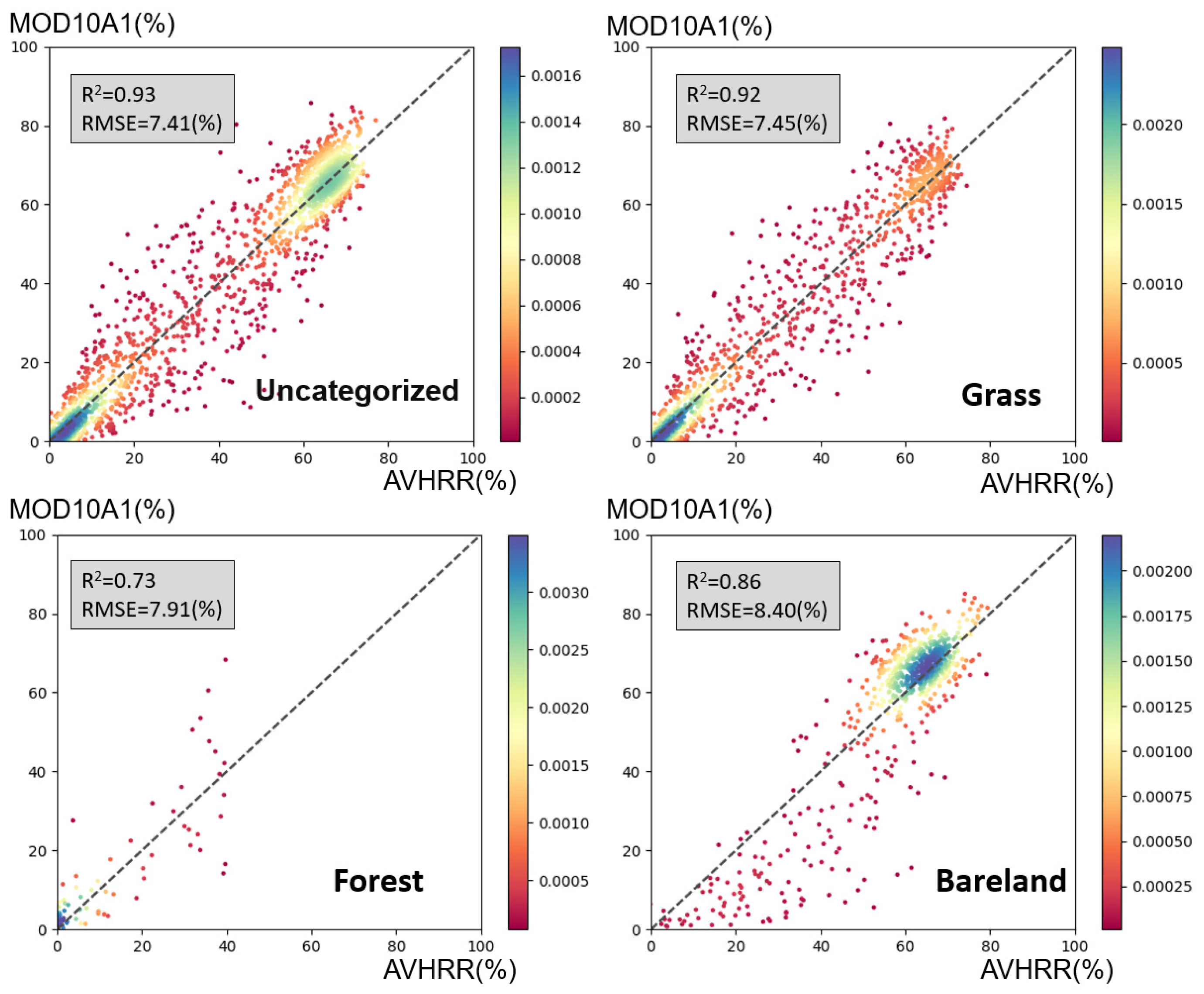
2.5. Land-Cover Type

According to previous studies [39,40], the complexity of surface conditions affects snow cover inversion accuracy. Surface conditions are primarily classified into two categories: topographic conditions and vegetation cover conditions. Topography mainly relates to elevation and slope. Vegetation cover conditions usually refer to vegetation types. For instance, in forest areas, trees will partially obscure snow-covered surface, and the effect of trees should be considered when mapping snow cover in forests, otherwise the snow cover in forested areas may be underestimated, such as the results observed by Solberg et al. in Norway [41]. For the effect of elevation, we used DEM data in representing elevation and also generated slope data based on DEM data. For the effect of surface vegetation cover, we used MCD10C1 land-cover type products based on MODIS data to reflect the surface vegetation cover types. Based on previous research [22], we roughly classified the vegetation cover types as forest, grassland or bareland.

3. Methods

The framework of this study mainly consists of three parts: data preprocessing, dataset production and accuracy validation (Figure 2). Data preprocessing includes quality control, cloud detection and the construction of fishnet. Quality control is primarily based on QA data from AVH09C1 to obtain valid pixels. Cloud detection will be detailed in Section 3.1. Due to the different resolutions between AVH09C1 and MOD10A1, and the much lower spatial resolution of AVH09C1 compared to MOD10A1, we construct fishnet (vector data) based on AVH09C1 to calculate statistical values for fitting and accuracy evaluation work. Dataset production mainly involves fitting core formulas and comparative analysis, with detailed content presented in Section 3.2. Accuracy analysis relies primarily on MOD10A1, ground observation data and ERA5 data, while also examining the stability of accuracy under different land surface vegetation cover types, elevations and slope conditions.

3.1. Cloud Detection

Due to potential issues of significant cloud cover overestimation in AVHRR [21,22], many studies have re-identified clouds, leading us to not directly adopt the cloudy flags. Cloud detection using AVHRR data remains a challenge due to the limited number of spectral bands. Effective cloud detection is crucial as it directly impacts the inversion results of target features, especially since the reflectance of snow in the visible spectrum overlaps with cloud altitudes. Currently, there are two mainstream methods for cloud monitoring: one categorizes clouds into high, medium, low and thin clouds, setting different thresholds for different cloud types [42]. Another approach, represented by Hori’s work, differentiates cloud monitoring between alpine and non-alpine regions and has achieved global cloud monitoring. Chen et al.’s study in the Tibetan Plateau has confirmed the adaptability of Hori’s method in the region [22]. Furthermore, Hao et al. have conducted a spectral analysis of cloud characteristics over China based on Hori’s method, making adjustments primarily focused on the threshold selection between BT3 and BT4 [23]. This study integrates the identification methods of Hori and Hao, presenting the following cloud identification method (as in

Table 3. Cloud detection tests and corresponding thresholds.

Target	Switch	DEM	SR1	SR2	SR3	SR1-SR2	NDVI	NDSI	BT4(K)	BT3-BT4	BT3-BT4	BT4-BT5
DEM > 300 m&BT11 < 260 K	On	<3000							≥240	>14.5	>19.5
	On	≥300							≥240	>15.5	>20
	On								<240	>21.5	>31
	On				>0.1	>−0.02		<0.88		>25.5	>33.5
	Off						>0.5		>288
	Off								>310
DEM < 300 m&BT11 ≥ 260 K	On								<260	>14	>16
	On					>−0.02			<310	>10.5	>16.5
	On		>0.3			>−0.02			<293	>11.5	>17.5
	On			>0.4		>−0.03			<293	>11.5	>18	>−1
	On			>0.4					<278	>11.5	>19.5	>−1
	On		>0.3		>0.2				<263	>11.5	>18
	Off						>0.5		>288
	Off								>310
	Off	>1000	<0.4			<−0.04			>275

). The cloud detector scans from the top to the bottom of the list for each target; a flag switch set to on indicates “cloudy”, while off indicates “no cloud”. A total of nine variables are used for cloud identification. It is important to note that NDSI_AVHRR is a variant of NDSI, using the 3.7 μm infrared band instead of the 1.6 μm near-infrared band.

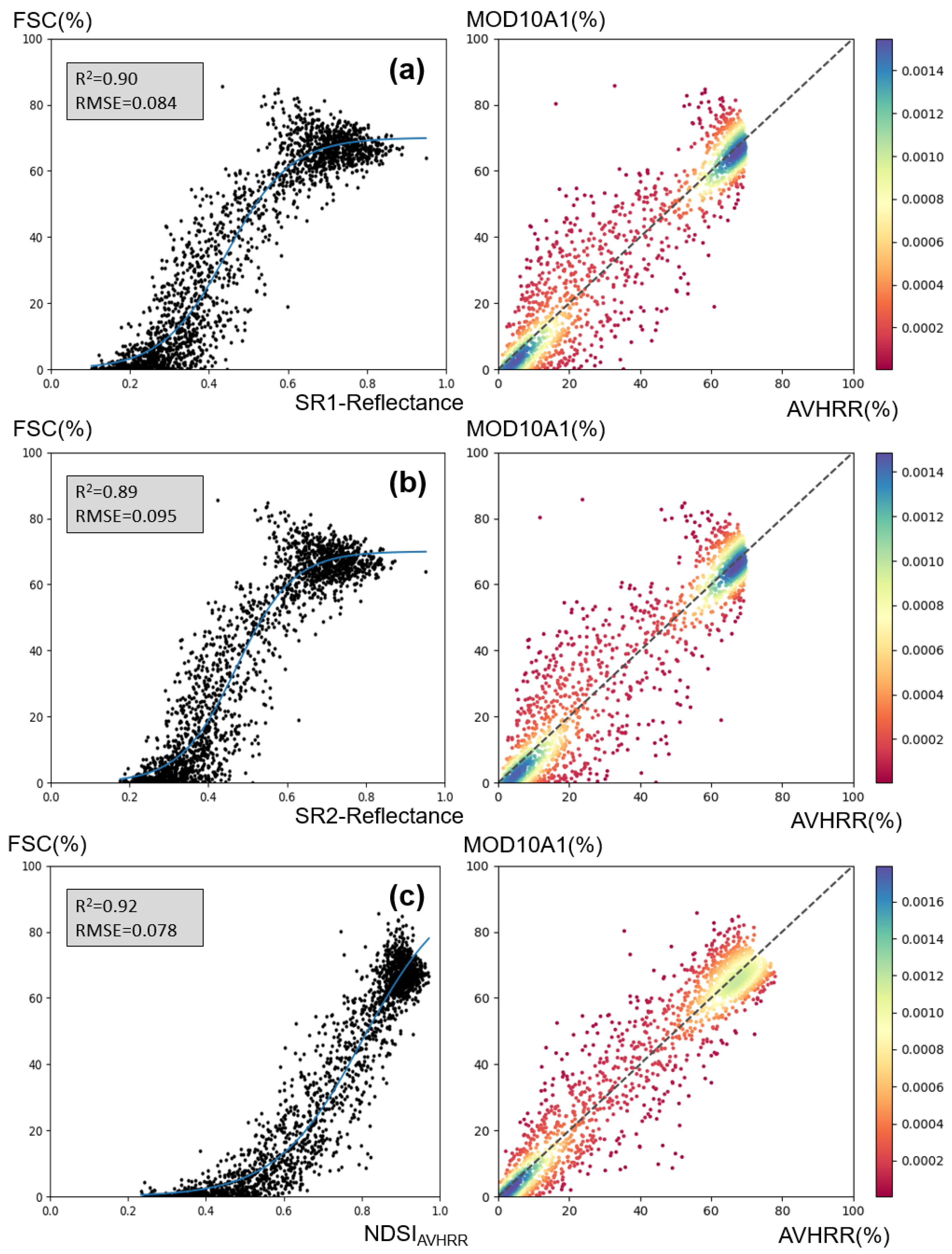
3.2. Inversion Algorithm of AVHRR FSC

We first selected SR1 and SR2 along with NDSI_AVHRR for fitting the snow cover percentage. By examining the distribution characteristics of the scatter plots, we performed both linear and logistic model fittings on the results. All pixel-based sampling points are averaged every 10 values to better illustrate the fitting effect. The findings indicate that the logistic model provided a better fit for B1, B2 and NDSIAVHRR. Among these, NDSIAVHRR achieved the best fitting results, with an R-squared and RMSE (Root Mean Square Error) of 0.92 and 0.078, respectively; B2 showed the poorest fit, with an R-squared and RMSE of 0.89 and 0.095, respectively, while B1’s results were intermediate. Both in terms of R-squared and RMSE, NDSI_AVHRR exhibited the best fitting results, although the outcomes of the three fitting parameters were very close. Ultimately, we selected NDSI_AVHRR as the key parameter for the inversion of snow cover percentage.

$$FSC=\frac{89.13\times e^{1.11+7.74\times {NDSI}_{AVHRR}}}{1+e^{1.11+7.74\times {NDSI}_{AVHRR}}}$$

(1)

The above formula can be regard as the vanilla algorithm. Although it achieves a high fitting effect, it does not consider the influence of the complex state of the ground surface on the snowpack inversion. In order to recognize these influences, we add other factors to improve the algorithm. According to previous studies, the main influences on snow cover inversion are elevation, slope, surface vegetation type and seasonal influence. Among them, the seasonal influence is mainly the difference in inversion models caused by different surface temperatures, and here we use BT4 as a rough characterization of surface temperature, combined with elevation and slope, which are continuous variables, and we use them together with NDSIAVHRR as variables in the logistic model. Multivariate fitting was performed separately for different vegetation cover types. The fitting results showed that the fitting results considering multiple factors were better than Equation (1). Further, we fitted the model for different vegetation cover types. Grassland had the best fit, followed by bare ground and forest, but all arrived at higher R-square, while RMSE was maintained at a low level, and finally, we used Equations (3)–(5) as the official inverse model (regarded as the improved algorithm).

$${FSC}_{Uncategorized}^{\prime }=\frac{80.88\times e^{f({NDSI}_{AVHRR},BT4,DEM,SLOP)}}{1+e^{f({NDSI}_{AVHRR},BT4,DEM,SLOP)}}$$

(2)

$$f\left({NDSI}_{AVHRR},BT4,DEM,SLOP\right)=10.90\times {NDSI}_{AVHRR}+6.23\times BT4+5.08\times DEM+1.06\times SLOP-12.58$$

$${FSC}_{Grass}^{*}=\frac{79.98\times e^{f_{grass}({NDSI}_{AVHRR},BT4,DEM,SLOP)}}{1+e^{f_{grass}({NDSI}_{AVHRR},BT4,DEM,SLOP)}}$$

(3)

$$f_{grass}\left({NDSI}_{AVHRR},BT4,DEM,SLOP\right)=10.30\times {NDSI}_{AVHRR}+1.42\times BT4+1.49\times DEM+0.75\times SLOP-8.00$$

$${FSC}_{Forest}^{*}=\frac{40.10\times e^{f_{forest}({NDSI}_{AVHRR},BT4,DEM,SLOP)}}{1+e^{f_{forest}({NDSI}_{AVHRR},BT4,DEM,SLOP)}}$$

(4)

$$f_{forest}\left({NDSI}_{AVHRR},BT4,DEM,SLOP\right)=17.63\times {NDSI}_{AVHRR}+228.79\times BT4+74.15\times DEM-0.47\times SLOP-96.29$$

$${FSC}_{bareland}^{*}=\frac{74.47\times e^{f_{bareland}({NDSI}_{AVHRR},BT4,DEM,SLOP)}}{1+e^{f_{bareland}({NDSI}_{AVHRR},BT4,DEM,SLOP)}}$$

(5)

$$f_{bareland}\left({NDSI}_{AVHRR},BT4,DEM,SLOP\right)=21.60\times {NDSI}_{AVHRR}+56.11\times BT4+5.09\times DEM+1.71\times SLOP-34.50$$

Equation (2) incorporates the influences of topography and surface temperature variations. Equations (3)–(5) present the fitting results under various surface vegetation cover conditions.

Comparing the results of Figure 3 and Figure 4, when elevation, slope and BT4 are added as variables, R-squared and RMSE are improved. Figure 4 also shows the fitting results under different vegetation cover types, among which Grass has the widest distribution and the largest number of sampling points on the Tibetan Plateau, and has the best fitting effect, with R-squared and RMSE reaching 0.92 and 0.0745, respectively. Forest is not the main vegetation cover type, but the R-squared and RMSE also reach 0.73 and 0.0745, respectively. Finally, we used Equations (3)–(5) as the improved algorithms for the AVHRR-FSC dataset.

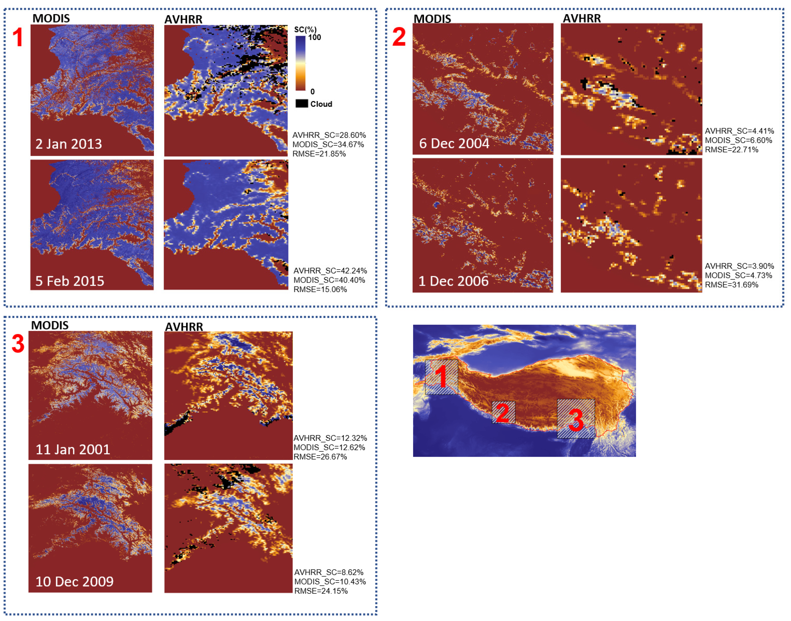
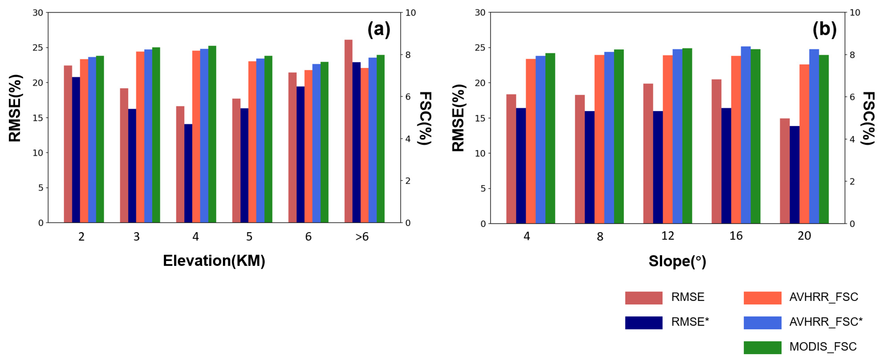
4. Accuracies of the AVHRR FSC Product

We compared the FSC inversion results of both the vanilla algorithm and the improved algorithm for six temporal phases between AVHRR and MODIS. As shown in Figure 5, across three test areas on the Tibetan Plateau the trends in snow cover percentage distribution were largely consistent between the two, with areas identified as cloudy in AVHRR also marked as non-snow in corresponding MODIS data, suggesting an alignment in cloud identification outcomes. This indicates the snow detection algorithm’s spatial reliability.

Figure 5 presents a comparison between AVHRR-FSC images of the vanilla algorithm and sub-pixel snow mapping images of MOD10A1. The visual comparison highlights differences in snow distribution, suggesting that significant discrepancies would question the sub-pixel snow spectroscopy’s reliability. Based on Figure 4, snow distribution from a visual interpretation of AVHRR/2 images corresponds with sub-pixel snow mapping outcomes, further affirming the sub-pixel snow mapping algorithm’s validity.

Additionally, we analyzed the standard deviation between AVHRR and MOD10A1 data for these phases, finding the largest standard deviation to be 28.68 and the smallest to be 15.05%. The most significant difference in snow-covered area among the test sites occurred on 14 December 2014, at less than 4%, with all other discrepancies below 3%. These findings, from both spatial distribution and statistical metrics, demonstrate a high congruence between AVHRR and MOD10A1 products.

Although Figure 5 demonstrates that the vanilla algorithm achieves high accuracy, the improved algorithm obtains a better result (Figure 6). For all six datasets, the snow cover area from the improved algorithm is closer to MOD10A1. Taking the time-phase data of 10 December 2009 and 6 December 2004 as examples, the vanilla algorithm recognizes the snow cover area of 8.62% and 4.41%, respectively, while the improved algorithm recognizes snow coverage of 11.26% and 6.04%, respectively. Despite the high RMSE values for both the vanilla and improved algorithms, it is important to note that RMSE values are calculated based on pixel size. This calculation method is over stringent due to the differences in spatial resolution between AVHRR and MODIS data. Even a minor misalignment in geographic coordinates can significantly increase the RMSE value, making it more appropriate as a reference rather than as an absolute measure of accuracy. Nevertheless, the statistical values of snow-covered areas and the results from visual interpretation exhibit a high degree of consistency between AVHRR-FSC data and MOD10A1.

To provide a more comprehensive comparison of the accuracy between the vanilla algorithm and the improved algorithm, we evaluated their performance under varying conditions of elevation, slope and vegetation cover types. As illustrated in Figure 7, regardless of elevation or slope, the RMSE remained below 30%. Under different elevation and slope conditions, the improved algorithm consistently exhibited lower RMSE values compared to the vanilla algorithm, and its estimates of snow-covered area were more closely aligned with MOD10A1 data.

In various elevation intervals, the RMSE values for both the vanilla and improved algorithms were highest at elevations below 2 km and above 6 km, with the lowest values occurring between 2 and 3 km. Regarding slope, the RMSE of the vanilla algorithm initially increased and then decreased, peaking for slopes between 12° and 16°, and reaching its lowest point for slopes between 16° and 20°. In contrast, the RMSE of the improved algorithm remained consistently lower than that of the vanilla algorithm within the 0° to 16° slope range, without significant variation, indicating greater stability.

As shown in Figure 8, the RMSE for different vegetation cover types remains below 20%. The RMSE of the improved algorithm is consistently lower than that of the baseline algorithm, and its snow cover area is closer to that of MOD10A1. For both the baseline and the improved algorithms, bareland exhibits the lowest RMSE, although the differences among the three are minimal. Based on comprehensive analysis from multiple perspectives, the improved algorithm outperforms the baseline algorithm. Therefore, we have adopted the improved algorithm as the core algorithm for the AVHRR-FSC dataset.

After completing the creation of the AVHRR-FSC dataset for the years 1982–2020, we used ground observation data and reanalysis data as supplementary validation methods. We employed snow-depth measurement data from 103 sites over 13 years, provided by the China Meteorological Administration (CMA), to validate our new AVHRR snow product. The overview of the validation results, as presented in

Table 4. The validation results of the AVHRR_FSC* based on ground snow-depth measurements.

Year	AVHRRsnow~Stationsnow	AVHRRnon-snow~Stationsnow	AVHRRsnow~Stationnon-snow	AVHRRnon-now~Stationnon-snow	K	Recall
2000	2007	17,183	423	15,169	0.07	0.83
2001	1615	17,730	350	15,276	0.06	0.82
2002	1748	17,749	286	15,010	0.06	0.86
2003	1252	16,970	276	12,265	0.04	0.82
2004	1532	18,666	329	13,521	0.04	0.82
2005	2324	18,896	392	13,261	0.07	0.86
2006	2038	18,702	579	13,673	0.05	0.79
2007	1447	17,211	334	16,267	0.05	0.81
2008	2412	18,060	287	14,598	0.08	0.90
2009	1687	17,178	344	16,115	0.06	0.83
2010	1079	17,772	346	16,367	0.03	0.76
2011	2123	17,394	766	15,786	0.06	0.73
2012	3737	16,459	1943	13,810	0.06	0.66

, shows that although kappa coefficients were generally low, the recall values were significantly higher. Notably, the peak recall value was recorded in 2008 at 0.90, while the lowest was in 2012, at 0.66, with the recall values for the other years all above 0.73. This indicates that the inversion results demonstrated a high level of stability.

The daily data from ERA5 for the year 2012 were used in our study. Due to cloud interference, the two datasets could not be directly compared. Therefore, we only compared the number of snow-covered pixels under cloud-free conditions between the two datasets, and the pixel count was evaluated based on AVHRR-FSC* snow pixels. The results indicate that the temporal variation trends of the two datasets are highly consistent (Figure 9). This indicates that the algorithm in this study has strong stability. It is important to note that both the ground observation data and the ERA5 data are based on observations from meteorological stations. There is a substantial difference in spatial scale between point data and raster data. Therefore, the accuracy assessment of the AVHRR-FSC* dataset needs to be comprehensively evaluated using Figure 6, Figure 7 and Figure 8, Table 4 and Figure 9.

5. Discussion

Through comparison and validation with MODIS and meteorological station data, we have confirmed that AVHRR-derived snow cover percentages exhibit high accuracy. It is important to note that MODIS and meteorological stations offer different perspectives for data validation. MODIS data is primarily used to assess the spatial consistency of snow inversion results. However, since the MOD10A1 does not contain cloud identification information [14], we did not directly evaluate the accuracy of cloud identification. The ability to correctly exclude cloud interference may represent one of the main challenges for AVHRR in snow inversion. In the example from 10 December 2009, in Figure 6, we observe that MODIS identified parts of the western Nyingchi Tanggula mountain as snow-free, whereas AVHRR results indicated significant cloud interference in this area, with more consistent identification results in other areas.

While many studies use meteorological station data to validate the accuracy of remotely sensed snow products [43,44,45], meteorological station snow-depth measurements are theoretically not ideal for validation purposes. This is because the stations provide point data, whereas AVHRR has a spatial resolution of 0.05°. Within a grid, the position of the station and the actual distribution of snow cover can greatly affect the accuracy assessment. However, the recall metric is very important for data from meteorological stations. This is because, if a station measures a certain snow depth, it confirms the presence of snow cover in that area, implying the AVHRR-detected snow cover percentage should be greater than 0. However, a snow depth of 0 at a station does not mean that there is no snow cover within the entire 0.05° × 0.05° grid of the station’s location. Therefore, for accuracy assessments based on meteorological stations, the significance of Recall is greater than that of Precision, Kappa and other evaluation metrics. In this study, the Recall values of the AVHRR snow cover product relative to meteorological station snow-depth data are at a high level, indicating that our algorithm has a high rate of snow cover detection.

Metsämäki et al., based on AVHRR and observational data, performed linear interpolation between reference reflectances under full snow cover conditions (SCA = 100%) and no snow conditions (SCA = 0%), different from the logistic model-based interpolation method used in our study, to estimate the Snow Cover Area (SCA) [46]. When validated against in situ SCA measurements from snow tracks, the overall accuracy was 85%, and when validated against snow measurements from meteorological stations, the accuracy was 64.4%. With the overall accuracy above 99% in our study (calculated from Figure 6), our sub-pixel snow mapping algorithm should be considered reliable and feasible.

The most significant finding of our study is the determination that the percentage of snow cover exhibits a logistic curve relationship with NDSI_AVHRR, whereas previous research results were often linear, such as when Hall et al. used a linear equation to simulate snow cover percentages with NDSI for MODIS data inversion. Additionally, spectral mixture models also differ from logistic models, which might relate to the data processing workflow and the selection of validation datasets. Nevertheless, this study has confirmed that the logistic model based on NDSI_AVHRR achieves high accuracy.

It is worth mentioning that Hüsler’s algorithm for inverting snow cover probability also utilized a logistic model and validated it with on-site data captured by network cameras. However, their logistic model was primarily used for calculating snow cover probability [19]. Logistic regression is more commonly applied in classification problems, and we employed it only because the fitting curve more accurately matched the characteristics of the scatter distribution. Currently, it is unclear whether their findings are in any way related to our research, which remains an area for future investigation.

The accuracy of snow cover detection algorithms is associated with various factors, such as elevation, surface roughness, etc. [47,48,49]. This study systematically analyzes, by distinguishing between the vanilla and improved algorithms, the effects of vegetation cover type and topographic elements on the accuracy of FSC inversion. The importance of considering these factors in the algorithm is demonstrated. In this study, slope is used as a proxy for surface roughness. Previous research has shown that elevation significantly influences accuracy, with snow detection precision tending to decrease as elevation increases. Despite the reduced snow detection accuracy at elevations above 6000 m in this study, this phenomenon is attributed to the unique geographical environment of the high mountain regions in Asia and the selection of validation images by date. Due to the high elevations in the high mountain regions of Asia, areas above 5000 m are predominantly covered by grasslands, leading to severe fragmentation of snow cover. This finding is consistent with previous research for elevations significantly below the 2000 to 6000 m range [49,50]. However, there was no significant decrease in accuracy within the 2000 to 6000 m range, and accuracy was lower at elevations below 2000 m. In the Tibetan Plateau region, areas below 2000 m, such as the Qaidam Basin and valleys on the southern edge of the plateau transitioning to the high plateau, experience climates transitioning from subtropical arid to subtropical forest climates to high plateau climates. Therefore, snow fragmentation is particularly severe in these areas. Additionally, it is important to note that the validation images selected were from the winter season when snow cover is more extensive, resulting in more concentrated snow cover in these areas and higher validation accuracy.

Due to cloud interference, the dataset created in this study cannot yet be directly applied to global change research [51]. Future work could involve the creation of long-term, cloud-free datasets through the fusion of multi-temporal and multi-source data. It is important to note that current long-term, cloud-free snow cover datasets are based on a binary snow/no-snow classification, utilizing multi-temporal fusion to mitigate some cloud effects and further integrating with passive microwave data to completely eliminate cloud influences [52,53,54]. However, for snow cover percentage data, while multi-temporal fusion allows for averaging pixel values, establishing a conversion relationship between snow-depth measurements and snow cover percentages when fusing with passive microwave data remains a technical challenge and a potential direction for future research.

In this study, we used MODIS snow products as training samples instead of selecting higher-resolution TM data, as many studies did, which could be seen as contentious. It is worth mentioning that our choice of the MODIS dataset was driven by two main reasons. Firstly, the MODIS snow product has undergone numerous iterations and updates, and its accuracy has been validated across many global regions, offering strong reliability [44,55,56]. Secondly, using MODIS as a training sample allows for easier balancing of RMSE to ensure consistency between AVHRR and MODIS inversion results, laying the groundwork for the next step of creating a long-term AVHRR-MODIS-VIIRS dataset. In the future, we plan to reference the NDVI dataset to create a global long-term FSC data product starting from 1981 and spanning over 40 years.

6. Conclusions

This study developed a snow cover dataset for the Tibetan Plateau region based on the long-term AVHRR dataset. Using MODIS data as ground truth, we fitted Bands 1, 2 and NDSI_AVHRR, and the results indicated that Band 1’s logistic curve fitting was the most optimal, achieving an R-squared of 0.9 for the training dataset and an RMSE of less than 0.5 for the prediction dataset. Furthermore, we analyzed the influence of factors such as surface vegetation cover type, elevation and slope on the algorithm by distinguishing between the vanilla algorithm and the improved algorithm. We assessed the importance of these factors and ultimately adopted the improved algorithm as the core algorithm for the AVHRR-FSC dataset. Through spatial comparison analysis with the MODIS dataset, we observed that the spatial distribution of AVHRR snow cover inversion results was consistent with those from MOD10A1, with a standard deviation of less than 0.2 for each spatial pixel. Considering that terrain might impact inversion accuracy, we analyzed accuracy under different elevation conditions, revealing that consistency between AVHRR and MOD10A1 inversion results increased with elevation. Comparison analysis with actual meteorological station data showed that, except for a Recall value of 0.66 in 2012, all other values were greater than 0.73, indicating that most snow-covered areas were detected. Additionally, the results also show a high degree of consistency with ERA5. This study demonstrates the feasibility of AVHRR inversion for snow cover percentage and provides the optimal fitting curve. The operational snow inversion technique designed in this study lays the foundation for future global AVHRR snow cover percentage product development.

References

1. Simpson, J.J.; Stitt, J.R.; Sienko, M. Improved Estimates of the Areal Extent of Snow Cover from AVHRR Data. J. Hydrol. 1998, 204, 1–23. [Google Scholar] [CrossRef]
2. Kelly, R.E.J.; Chang, A.T.C. Development of a Passive Microwave Global Snow Depth Retrieval Algorithm for Special Sensor Microwave Imager (SSM/I) and Advanced Microwave Scanning Radiometer-EOS (AMSR-E) Data. Radio Sci. 2003, 38, 41. [Google Scholar] [CrossRef]
3. Hall, D.K.; Riggs, G.A.; Salomonson, V.V.; DiGirolamo, N.E.; Bayr, K.J. MODIS Snow-Cover Products. Remote Sens. Environ. 2002, 83, 181–194. [Google Scholar] [CrossRef]
4. Riggs, G.A.; Hall, D.K.; Román, M.O. Overview of NASA’s MODIS and Visible Infrared Imaging Radiometer Suite (VIIRS) Snow-Cover Earth System Data Records. Earth Syst. Sci. Data 2017, 9, 765–777. [Google Scholar] [CrossRef]
5. Marchane, A.; Jarlan, L.; Hanich, L.; Boudhar, A.; Gascoin, S.; Tavernier, A.; Filali, N.; Le Page, M.; Hagolle, O.; Berjamy, B. Assessment of Daily MODIS Snow Cover Products to Monitor Snow Cover Dynamics over the Moroccan Atlas Mountain Range. Remote Sens. Environ. 2015, 160, 72–86. [Google Scholar] [CrossRef]
6. Hüsler, F.; Jonas, T.; Riffler, M.; Musial, J.P.; Wunderle, S. A Satellite-Based Snow Cover Climatology (1985–2011) for the European Alps Derived from AVHRR Data. Cryosph. 2014, 8, 73–90. [Google Scholar] [CrossRef]
7. Helfrich, S.R.; McNamara, D.; Ramsay, B.H.; Baldwin, T.; Kasheta, T. Enhancements to, and Forthcoming Developments in the Interactive Multisensor Snow and Ice Mapping System (IMS). Hydrol. Process. An Int. J. 2007, 21, 1576–1586. [Google Scholar] [CrossRef]
8. Robinson, D.A.; Dewey, K.F.; Heim, R.R. Global Snow Cover Monitoring: An Update. Bull.-Am. Meteorol. Soc. 1993, 74, 1689–1696. [Google Scholar] [CrossRef]
9. Wang, X.; Xie, H.; Liang, T. Evaluation of MODIS Snow Cover and Cloud Mask and Its Application in Northern Xinjiang, China. Remote Sens. Environ. 2008, 112, 1497–1513. [Google Scholar] [CrossRef]
10. Stroeve, J.; Box, J.E.; Gao, F.; Liang, S.; Nolin, A.; Schaaf, C. Accuracy Assessment of the MODIS 16-Day Albedo Product for Snow: Comparisons with Greenland in Situ Measurements. Remote Sens. Environ. 2005, 94, 46–60. [Google Scholar] [CrossRef]
11. Solberg, R.; Wangensteen, B.; Amlien, J.; Koren, H.; Metsämäki, S.; Nagler, T.; Luojus, K.; Pulliainen, J. A New Global Snow Extent Product. In Proceedings of the Proceedings of ESA Living Planet Symposium, ESA Special Publication SP-686, Bergen, Norway, 26 June–2 July 2010. [Google Scholar]
12. Ramsay, B.H. The Interactive Multisensor Snow and Ice Mapping System. Hydrol. Process. 1998, 12, 1537–1546. [Google Scholar] [CrossRef]
13. Hall, D.K.; Salomonson, V.V.; Riggs, G.A. MODIS/Terra Snow Cover 8-Day L3 Global 500m Grid; Version 5; Tile h12v12; National Snow and Ice Data Center: Boulder, CO, USA, 2006. [Google Scholar]
14. Riggs, G.A.; Hall, D.K.; Román, M.O. MODIS Snow Products Collection 6 User Guide; National Snow and Ice Data Center: Boulder, CO, USA, 2015; Volume 66. [Google Scholar]
15. Zhao, Q.; Hao, X.; He, D.; Wang, J.; Li, H.; Wang, X. The Relationship between the Temporal and Spatial Changes of Snow Cover and Climate and Vegetation in Northern Xinjiang from 1980 to 2019. Remote Sens. Technol. Appl. 2022, 36, 1247–1258. [Google Scholar]
16. Qiu, B.; Li, W.; Wang, X.; Shang, L.; Song, C.; Guo, W.; Zhang, Y. Satellite-Observed Solar-Induced Chlorophyll Fluorescence Reveals Higher Sensitivity of Alpine Ecosystems to Snow Cover on the Tibetan Plateau. Agric. For. Meteorol. 2019, 271, 126–134. [Google Scholar] [CrossRef]
17. Alkama, R.; Forzieri, G.; Duveiller, G.; Grassi, G.; Liang, S.; Cescatti, A. Vegetation-Based Climate Mitigation in a Warmer and Greener World. Nat. Commun. 2022, 13, 606. [Google Scholar] [CrossRef]
18. Khlopenkov, K.V.; Trishchenko, A.P. SPARC: New Cloud, Snow, and Cloud Shadow Detection Scheme for Historical 1-Km AVHHR Data over Canada. J. Atmos. Ocean. Technol. 2007, 24, 322–343. [Google Scholar] [CrossRef]
19. Hüsler, F.; Jonas, T.; Wunderle, S.; Albrecht, S. Validation of a Modified Snow Cover Retrieval Algorithm from Historical 1-Km AVHRR Data over the European Alps. Remote Sens. Environ. 2012, 121, 497–515. [Google Scholar] [CrossRef]
20. Zhou, H.; Aizen, E.; Aizen, V. Deriving Long Term Snow Cover Extent Dataset from AVHRR and MODIS Data: Central Asia Case Study. Remote Sens. Environ. 2013, 136, 146–162. [Google Scholar] [CrossRef]
21. Hori, M.; Sugiura, K.; Kobayashi, K.; Aoki, T.; Tanikawa, T.; Kuchiki, K.; Niwano, M.; Enomoto, H. A 38-Year (1978–2015) Northern Hemisphere Daily Snow Cover Extent Product Derived Using Consistent Objective Criteria from Satellite-Borne Optical Sensors. Remote Sens. Environ. 2017, 191, 402–418. [Google Scholar] [CrossRef]
22. Chen, X.; Long, D.; Liang, S.; He, L.; Zeng, C.; Hao, X.; Hong, Y. Developing a Composite Daily Snow Cover Extent Record over the Tibetan Plateau from 1981 to 2016 Using Multisource Data. Remote Sens. Environ. 2018, 215, 284–299. [Google Scholar] [CrossRef]
23. Hao, X.; Huang, G.; Che, T.; Ji, W.; Sun, X.; Zhao, Q.; Zhao, H.; Wang, J.; Li, H.; Yang, Q. The NIEER AVHRR Snow Cover Extent Product over China - A Long-Term Daily Snow Record for Regional Climate Research. Earth Syst. Sci. Data 2021, 13, 4711–4726. [Google Scholar] [CrossRef]
24. Wang, S.; Wang, X.; Chen, G.; Yang, Q.; Wang, B.; Ma, Y.; Shen, M. Complex Responses of Spring Alpine Vegetation Phenology to Snow Cover Dynamics over the Tibetan Plateau, China. Sci. Total Environ. 2017, 593, 449–461. [Google Scholar] [CrossRef]
25. Ranzi, R.; Grossi, G.; Bacchi, B. Ten Years of Monitoring Areal Snowpack in the Southern Alps Using NOAA-AVHRR Imagery, Ground Measurements and Hydrological Data. Hydrol. Process. 1999, 13, 2079–2095. [Google Scholar] [CrossRef]
26. Wang, L.; Sharp, M.; Brown, R.; Derksen, C.; Rivard, B. Evaluation of Spring Snow Covered Area Depletion in the Canadian Arctic from NOAA Snow Charts. Remote Sens. Environ. 2005, 95, 453–463. [Google Scholar] [CrossRef]
27. Harrison, A.R.; Lucas, R.M. Multi-Spectral Classification of Snow Using NOAA AVHRR Imagery. Int. J. Remote Sens. 1989, 10, 907–916. [Google Scholar] [CrossRef]
28. Pu, Z.; Xu, L.; Salomonson, V.V. MODIS/Terra Observed Seasonal Variations of Snow Cover over the Tibetan Plateau. Geophys. Res. Lett. 2007, 34, L06706. [Google Scholar] [CrossRef]
29. You, Q.; Wu, T.; Shen, L.; Pepin, N.; Zhang, L.; Jiang, Z.; Wu, Z.; Kang, S.; AghaKouchak, A. Review of Snow Cover Variation over the Tibetan Plateau and Its Influence on the Broad Climate System. Earth-Sci. Rev. 2020, 201, 103043. [Google Scholar] [CrossRef]
30. Vermote, E.; Justice, C.; Csiszar, I.; Eidenshink, J.; Myneni, R.; Baret, F.; Masuoka, E.; Wolfe, R.; Claverie, M. NOAA Climate Data Record (CDR) of AVHRR Surface Reflectance; Version 5; NOAA National Centers for Environmental Information: Washington, DC, USA, 2019. [Google Scholar]
31. Franch, B.; Vermote, E.F.; Roger, J.-C.; Murphy, E.; Becker-Reshef, I.; Justice, C.; Claverie, M.; Nagol, J.; Csiszar, I.; Meyer, D. A 30+ Year AVHRR Land Surface Reflectance Climate Data Record and Its Application to Wheat Yield Monitoring. Remote Sens. 2017, 9, 296. [Google Scholar] [CrossRef] [PubMed]
32. Rittger, K.; Painter, T.H.; Dozier, J. Assessment of Methods for Mapping Snow Cover from MODIS. Adv. Water Resour. 2013, 51, 367–380. [Google Scholar] [CrossRef]
33. Wang, X.; Zheng, H.; Chen, Y.; Liu, H.; Liu, L.; Huang, H.; Liu, K. Mapping Snow Cover Variations Using a MODIS Daily Cloud-Free Snow Cover Product in Northeast China. J. Appl. Remote Sens. 2014, 8, 84681. [Google Scholar] [CrossRef]
34. Gao, Y.; Xie, H.; Lu, N.; Yao, T.; Liang, T. Toward Advanced Daily Cloud-Free Snow Cover and Snow Water Equivalent Products from Terra–Aqua MODIS and Aqua AMSR-E Measurements. J. Hydrol. 2010, 385, 23–35. [Google Scholar] [CrossRef]
35. Tong, J.; Déry, S.J.; Jackson, P.L. Interrelationships between MODIS/Terra Remotely Sensed Snow Cover and the Hydrometeorology of the Quesnel River Basin, British Columbia, Canada. Hydrol. Earth Syst. Sci. 2009, 13, 1439–1452. [Google Scholar] [CrossRef]
36. Hersbach, H.; Bell, B.; Berrisford, P.; Hirahara, S.; Horányi, A.; Muñoz-Sabater, J.; Nicolas, J.; Peubey, C.; Radu, R.; Schepers, D. The ERA5 Global Reanalysis. Q. J. R. Meteorol. Soc. 2020, 146, 1999–2049. [Google Scholar] [CrossRef]
37. Lei, Y.; Letu, H.; Shang, H.; Shi, J. Cloud Cover over the Tibetan Plateau and Eastern China: A Comparison of ERA5 and ERA-Interim with Satellite Observations. Clim. Dyn. 2020, 54, 2941–2957. [Google Scholar] [CrossRef]
38. Lei, Y.; Pan, J.; Xiong, C.; Jiang, L.; Shi, J. Snow Depth and Snow Cover over the Tibetan Plateau Observed from Space in against ERA5: Matters of Scale. Clim. Dyn. 2023, 60, 1523–1541. [Google Scholar] [CrossRef]
39. Shreve, C.M.; Okin, G.S.; Painter, T.H. Indices for Estimating Fractional Snow Cover in the Western Tibetan Plateau. J. Glaciol. 2009, 55, 737–745. [Google Scholar] [CrossRef]
40. Dietz, A.J.; Kuenzer, C.; Gessner, U.; Dech, S. Remote Sensing of Snow–a Review of Available Methods. Int. J. Remote Sens. 2012, 33, 4094–4134. [Google Scholar] [CrossRef]
41. Solberg, R.; Hiltbrunner, D.; Koskinen, J.; Guneriussen, T.; Rautiainen, K.; Hallikainen, M. Snow Algorithms and Products-Review and Recommendations for Research and Development; Norwegian Computing Center: Oslo, Norway, 1997. [Google Scholar]
42. Zhu, J.; Cao, S.; Shang, G.; Shi, J.; Wang, X.; Zheng, Z.; Liu, C.; Yang, H.; Xie, B. Subpixel Snow Mapping Using Daily AVHRR/2 Data over Qinghai–Tibet Plateau. Remote Sens. 2022, 14, 2899. [Google Scholar] [CrossRef]
43. Orsolini, Y.; Wegmann, M.; Dutra, E.; Liu, B.; Balsamo, G.; Yang, K.; de Rosnay, P.; Zhu, C.; Wang, W.; Senan, R. Evaluation of Snow Depth and Snow Cover over the Tibetan Plateau in Global Reanalyses Using in Situ and Satellite Remote Sensing Observations. Cryosph. 2019, 13, 2221–2239. [Google Scholar] [CrossRef]
44. Parajka, J.; Blöschl, G. Validation of MODIS Snow Cover Images over Austria. Hydrol. Earth Syst. Sci. 2006, 10, 679–689. [Google Scholar] [CrossRef]
45. Simic, A.; Fernandes, R.; Brown, R.; Romanov, P.; Park, W. Validation of VEGETATION, MODIS, and GOES+ SSM/I Snow-cover Products over Canada Based on Surface Snow Depth Observations. Hydrol. Process. 2004, 18, 1089–1104. [Google Scholar] [CrossRef]
46. Metsämäki, S.; Vepsäläinen, J.; Pulliainen, J.; Sucksdorff, Y. Improved Linear Interpolation Method for the Estimation of Snow-Covered Area from Optical Data. Remote Sens. Environ. 2002, 82, 64–78. [Google Scholar] [CrossRef]
47. Veitinger, J.; Sovilla, B.; Purves, R.S. Influence of Snow Depth Distribution on Surface Roughness in Alpine Terrain: A Multi-Scale Approach. Cryosph. 2014, 8, 547–569. [Google Scholar] [CrossRef]
48. Parajka, J.; Dadson, S.; Lafon, T.; Essery, R. Evaluation of Snow Cover and Depth Simulated by a Land Surface Model Using Detailed Regional Snow Observations from Austria. J. Geophys. Res. Atmos. 2010, 115, D24117. [Google Scholar] [CrossRef]
49. Wu, X.; Naegeli, K.; Premier, V.; Marin, C.; Ma, D.; Wang, J.; Wunderle, S. Evaluation of Snow Extent Time Series Derived from Advanced Very High Resolution Radiometer Global Area Coverage Data (1982–2018) in the Hindu Kush Himalayas. Cryosph. 2021, 15, 4261–4279. [Google Scholar] [CrossRef]
50. Pan, F.; Jiang, L.; Zheng, Z.; Wang, G.; Cui, H.; Zhou, X.; Huang, J. Retrieval of Fractional Snow Cover over High Mountain Asia Using 1 Km and 5 Km AVHRR/2 with Simulated Mid-Infrared Reflective Band. Remote Sens. 2022, 14, 3303. [Google Scholar] [CrossRef]
51. Jing, Y.; Shen, H.; Li, X.; Guan, X. A Two-Stage Fusion Framework to Generate a Spatio–Temporally Continuous MODIS NDSI Product over the Tibetan Plateau. Remote Sens. 2019, 11, 2261. [Google Scholar] [CrossRef]
52. Huang, X.; Deng, J.; Wang, W.; Feng, Q.; Liang, T. Impact of Climate and Elevation on Snow Cover Using Integrated Remote Sensing Snow Products in Tibetan Plateau. Remote Sens. Environ. 2017, 190, 274–288. [Google Scholar] [CrossRef]
53. Hall, D.K.; Riggs, G.A.; Foster, J.L.; Kumar, S. V Development and Evaluation of a Cloud-Gap-Filled MODIS Daily Snow-Cover Product. Remote Sens. Environ. 2010, 114, 496–503. [Google Scholar] [CrossRef]
54. Kumar, S.V.; Peters-Lidard, C.D.; Arsenault, K.R.; Getirana, A.; Mocko, D.; Liu, Y. Quantifying the Added Value of Snow Cover Area Observations in Passive Microwave Snow Depth Data Assimilation. J. Hydrometeorol. 2015, 16, 1736–1741. [Google Scholar] [CrossRef]
55. Klein, A.G.; Barnett, A.C. Validation of Daily MODIS Snow Cover Maps of the Upper Rio Grande River Basin for the 2000–2001 Snow Year. Remote Sens. Environ. 2003, 86, 162–176. [Google Scholar] [CrossRef]
56. Hall, D.K.; Riggs, G.A. Accuracy Assessment of the MODIS Snow Products. Hydrol. Process. An Int. J. 2007, 21, 1534–1547. [Google Scholar] [CrossRef]
Figure 1. Study area and test areas for regression.
Remotesensing 16 02260 g001
Figure 2. Flowchart of AVHRR-FSC generation and accuracy analysis in this study.
Remotesensing 16 02260 g002
Figure 3. Linear fitting of SR1, SR2 and NDSIAVHRR with MOD10A1 for training data. The blue line represents the fit line, and the dash line represents the perfect prediction line. (a) the linear fitting of SR1 with MOD10A1; (b) the linear fitting of SR2 with MOD10A1; (c) the linear fitting of NDSIAVHRR with MOD10A1.
Remotesensing 16 02260 g003
Figure 4. Scatter density plots for Logistic fitting results after considering elevation, slop, BT4 and comparison of predicted values with MOD10A1. The four subplots are related to uncategorized, grass, forest and bareland for vegetation cover types. The dash line represents the perfect prediction line.
Remotesensing 16 02260 g004
Figure 5. Comparison of AVHRR_FSC (the vanilla algorithm) and MODIS_FSC mapping; AVHRR_FSC and MODIS_FSC stand for total snow cover area, and RMSE is pixel-based calculated. 1, 2, and 3 correspond to the three test areas.
Remotesensing 16 02260 g005
Figure 6. Comparison of AVHRR_FSC* (the improved algorithm) and MODIS_FSC mapping; AVHRR_FSC* and MODIS_FSC stand for total snow cover area, and RMSE is pixel-based calculated. 1, 2, and 3 correspond to the three test areas.
Remotesensing 16 02260 g006
Figure 7. Trends in RMSE of AVHRR FSC inversion results with elevation and slope variation, using MOD10A1 as the ground truth. RMSE and AVHRR_FSC stand for the vanilla algorithm, RMSE* and AVHRR_FSC* stand for the improved algorithm. (a) trends in RMSE of AVHRR FSC inversion results with elevation; (b) Trends in RMSE of AVHRR FSC inversion results with slop.
Remotesensing 16 02260 g007
Figure 8. Trends in RMSE of AVHRR FSC inversion results with different vegetation types, using MOD10A1 as the ground truth. RMSE and AVHRR_FSC stand for the vanilla algorithm, RMSE* and AVHRR_FSC* stand for improved algorithm.
Remotesensing 16 02260 g008
Figure 9. Snow cover pixel count of AVHRR-FSC* compared to ERA5. AVHRR-FSC* is the result of the improved algorithm. (a) shows the comparison of daily snow cover pixel count; (b) shows the consistency between the two datasets.
Remotesensing 16 02260 g009