Spatiotemporal Variabilities in Evapotranspiration of Alfalfa: A Case Study Using Remote Sensing METRIC and SSEBop Models and Eddy Covariance

Abstract

Prolonged drought exacerbated by climate change in the Mesilla Valley, one of the major agricultural areas of New Mexico, USA, is causing a shortage of surface water from the Rio Grande for irrigation. Farmers in the Valley are using groundwater for irrigation and complementing it with limited surface water from the river (Rio Grande). Managing irrigation water better is vital to sustaining agriculture in the Valley. Remote sensing (RS)-based crop evapotranspiration (ETa) models offer significant advantages over traditional methods. The ET maps generated by these RS models provide valuable information that can be used to manage irrigation water and crops in water-scarce areas. This study used METRIC and SSEBop RS models to map the ET of alfalfa on a private farm that is managed as commonly practiced in the Valley. The integrated ET values of the two models are compared to those of the ETa measured using the eddy covariance method. The comparison showed that 91.55% of the variability in SSEBop ETa estimates can be explained by the variability in the METRIC ETa estimates, and the variability in eddy covariance ETa can explain 93.07% of the variability in METRIC ETa and 86.01% in the SSEBop Eta estimates. Both METRIC and SSEBop reflected the ETa of alfalfa during full growth and harvesting periods. However, the absolute percent mean relative difference (MRD) of ET was higher for two out of three cuttings by SSEBop (>32%) compared to those for METRIC and eddy covariance. The spatiotemporal variabilities in crop ET estimates using METRIC and SSEBop showed a need to improve on-farm irrigation conveyance and on-the-field irrigation efficiency. Overall, RS models can provide spatiotemporal maps of ET that can be used for decision-making to manage irrigation water better and improve crop yield on a field, farm, and regional scale.

1. Introduction

Alfalfa (Medicago Sativa L.) is a highly versatile perennial forage legume crop that can be harvested multiple times throughout the growing season and can live from three to twelve years. Typically, farmers rotate alfalfa in three- or four-year increments to achieve a high-quality crop for its nutrient value as a staple food source for livestock. It is utilized in various forms, such as hay, silage, and pasture. Alfalfa is one of the major crops grown in the Mesilla Valley, New Mexico, and is one of the economically important crops in the State of New Mexico, USA [1]. According to the USDA agricultural statistics report [1], alfalfa ranked second by area behind pecans in the Mesilla Valley in 2017; about 77,000 ha of alfalfa hay valued at $171,000,000 was harvested in the state of New Mexico. A study by Lacefield et al. [2] found that approximately 80% of the alfalfa in the southern region of the United States is harvested for hay, with the rest being used for hay or baleage and only a small amount being gathered as greenchops. Horse producers use around 45% of this alfalfa, while the dairy industry accounts for about 40%, and beef cattle enterprises use 15%. Small quantities are also used for sheep, goats, and other farm animals.

In the Mesilla Valley, flooding is the most common method of irrigation for alfalfa. Irrigation water is primarily sourced from annually allocated surface water from the Rio (river) Grande, which is managed and distributed by the Elephant Butte Irrigation District (EBID) through a network of irrigation canals and supplemented by groundwater from privately owned irrigation wells when needed. Due to several years of drought in the region, farmers are now relying on groundwater for irrigation. Alfalfa requires a large amount of water to grow, and its evapotranspiration (ET) or “actual” ET (ETa) has been measured and reported in the literature. It should be noted, however, that the seasonal and annual ET values of alfalfa measured or reported from different studies should be considered with caution. The ET of alfalfa varies among alfalfa “varieties”, the length of the growing season (climate) of that particular region, the type of irrigation, soil moisture, farming practices, and other environmental factors. For example, Sammis [3] measured the ETa of alfalfa at three study sites and reported 1575 mm, 1739 mm, and 1749 mm per year using a non-weighing lysimeter in the Mesilla Valley in 1976. Boyko et al. [4], in another study, used the eddy covariance method to measure an ETa of alfalfa of 1309 mm for a total of 269 days in 2017. Wright [5] measured daily ETa of alfalfa for 7 years using weighing lysimeters at two study sites located at the Snake River Conservation Research Center east of Kimberly, Idaho, during the growing season from April through October.

The seasonal ETa of alfalfa averaged 1016 mm [5]. The alfalfa was harvested three times each year and was irrigated when needed. The harvests decreased the ETa to less than 25% of preharvest levels for approximately one week, and then an additional 1 to 2 weeks were needed to return to the potential ETa rates. Wagle et al. [6] measured a seasonal (April–October) ETa of 652 mm in 2016 and 734 mm in 2017 for non-irrigated alfalfa using the eddy covariance technique in central Oklahoma, USA. Djaman et al. [7] cited from the Food and Agriculture Manual FAO-56 that alfalfa water use varied from 615 mm to 1448 mm across the US Great Plains.

Measuring the ET of crops involves several direct and indirect methods. Some direct methods include using weighing and non-weighing lysimeters, soil moisture sensors (soil moisture depletion), eddy covariance, and the Bowen ratio. The indirect methods of estimating crop ET include climate-based approaches such as calculating the reference ET using the Penman–Monteith method [8] and then multiplying by the crop coefficient; the residual energy budget method, where ET is calculated as a residual in the energy budget; and the remote sensing-based methods. Remote sensing (RS) models have the potential to estimate crop ET over large areas in the absence of field-measured ET and limited meteorological data [9,10].

Various remote sensing methods have been utilized to determine crop ETa at different scales. The Moderate Resolution Imaging Spectroradiometer (MODIS) [11], Advanced Spaceborne Thermal Emission and Reflection Radiometer (ASTER) [12], and Landsat are satellite sensors that offer crucial information for evaluating evapotranspiration trends across vast regions. These remote sensing methods incorporate surface temperature, vegetation indices, and other parameters to estimate crop ETa [13,14]. Some of these RS methods include mapping evapotranspiration at high resolution with internalized calibration (METRIC) [9,10], the surface energy balance algorithm for land (SEBAL) [13,14], the operational simplified surface energy balance (SSEBop) [15], the surface energy balance system (SEBS) [16], the simplified surface energy balance index (SSEBI) [17], the two-source energy balance model (TSEB) [18], and the atmosphere–land exchange inverse (ALEXI) [19]. Recently, the OPENET and Google Earth Engine Evapotranspiration Flux (EEFlux) platforms have been introduced as automated tools to calculate the ET of crops [9,13,15,20,21,22,23,24,25,26]. A summarized description of the different remote sensing models can be found in [27,28,29,30]. Satellite remote sensing provides a broader view of the Earth’s land surface, complementing the limited range of ground-based observation systems. It is considered the most promising method for predicting ETa over large areas [31,32]. However, RS can be affected by atmospheric interference and significantly impact the quality of satellite data. Furthermore, the satellite’s low temporal resolution (time gaps between estimates of ET) is another issue that affects the quality of information to estimate daily ETa values. Estimating ETa by remote sensing can be costly, as it requires high-resolution data and special tools to process data.

A study by French et al. [33] was conducted using three remote sensing models to estimate alfalfa ET over the Central Arizona Irrigation and Drainage District (CAIDD) in 2008. The models used were the mapping of evapotranspiration with internalized calibration (METRIC), the two-source energy balance (TSEB), and the vegetation index ET for the US Southwest (VISW). They compared the results from the three models with the USDA-SW gravimetric ET data. The findings showed that the estimated seasonal ETa from the METRIC, TSEB, and VISW were 1317.4, 1746.1, and 1217.3 mm, respectively, compared to the USDA-SW gravimetric seasonal ET of 1887.7 mm. Djaman et al. [7] conducted a study to estimate the monthly and annual ET using the remote sensing-based OpenET platform for four different crops grown in the Navajo Agricultural Products Industry (NAPI) in NM, USA, from 2016 to 2020. The four major crops included alfalfa, maize, potatoes, and dry beans. The results revealed that alfalfa had the highest seasonal ETa of 1015.4 mm. Mkhwananzi and Chavez [34] compared the ETa of irrigated alfalfa estimated by the remote sensing METRIC model with ETa measured using a weighing lysimeter in the 2010 growing season and found a good correlation between them (R² ₌ 0.83 and RMSE of 0.14 mm/h). Madugunda et al. [35] compared the METRIC model ETa with the eddy covariance ETa of an irrigated alfalfa located southeast of Riyadh, Saudi Arabia. Their comparison showed a good agreement between the results, with an R² of 0.81 and RMSE of 0.13 mm/h. However, the comparison of ET on a daily basis resulted in an R² of 0.66 and RMSE of 4.15 mm. Wagle et al. [32] compared the MODIS ET with the eddy covariance ETa (R² of 0.73 and RMSE of 1.06 mm/day) of a non-irrigated alfalfa field in central Oklahoma, USA, for the growing season (April–October) of 2016 and 2017.

To sustain agriculture in the region and manage limited water resources, these remote sensing tools and techniques for decision-making are needed. The availability of remote sensing data and emerging model algorithms for estimating ETa, such as METRIC and SSEBop, allows for estimating and observing the ET of crops (i.e., ETa) on a spatiotemporal scale. The information they provide can then be used for decision-making to improve irrigation and manage soil nutrients, salinity, and crops on an individual field, farm, and even on a regional scale.

Two models, METRIC [9,10] and SSEBop [15], that use remote sensing data in combination with climate data to estimate alfalfa ETa were used in this study. These two models were selected due to their simplicity and because their ETa estimates have been compared well with ground measurements using other methods, such as the eddy covariance and lysimeter, as discussed earlier.

The objectives of this study were to i. compare the ETa of alfalfa estimated by the two models and with eddy covariance measurements and to determine if they can be used in the future for irrigation management and ii. map the spatiotemporal variability of alfalfa ETa on a farm-field scale. The aim was to determine if vital information can be attained from the spatiotemporal variability of ETa for decision-making to improve irrigation practices and management.

2. Materials and Methods

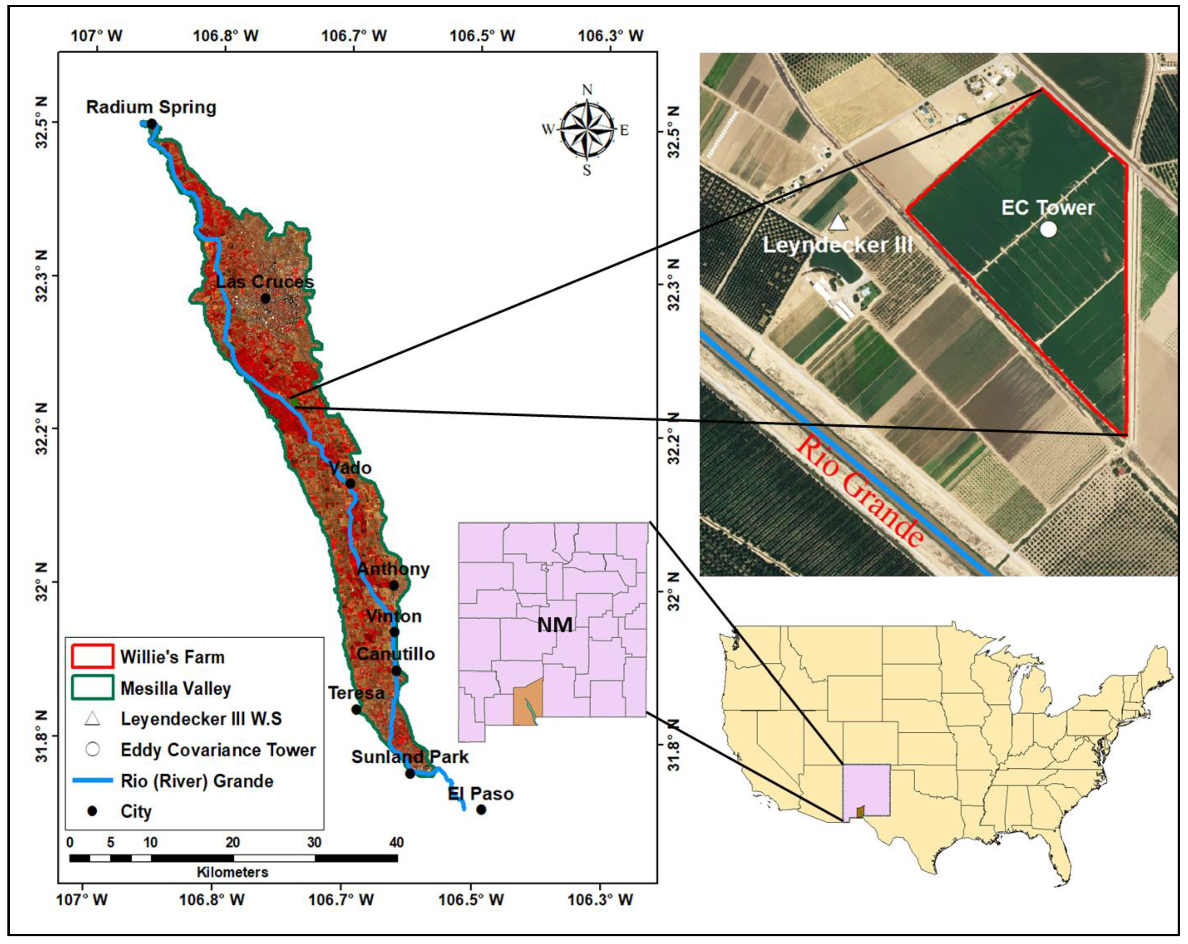
2.1. Description of the Study Area

An alfalfa farm named Willie’s Farm was used in this study and located (32°12′03.07″N and 106°44′09.90″, WGS84) in the Mesilla Valley in New Mexico, USA coordinate system. The Valley is dominated by agriculture and covers an area of about 47,000 ha, extending from Radium Spring to Sunland Park (Figure 1). The area was estimated by digitizing the Valley using a geographic information system (GIS) tool over a high-resolution (1 m) image from the US Geological Survey (USGS) National Agriculture Imagery Program (NAIP) website: https://earthexplorer.usgs.gov/, accessed on 19 October 2021 [36]. Farming land in the Valley covers about 65 percent of the total area, and the City of Las Cruces, small towns, and housing developments occupy the rest of the area. The Valley is widely recognized for its flourishing agricultural sector due to its fertile soil and available irrigation water from the Rio Grande. Agriculture in the region relies on water for irrigation from the Rio Grande when available and on groundwater during dry spells when water from the river is not available or enough to support crop production.

Willie’s Farm covers an area of 35.2 ha at an elevation of 1176 m AMSL and is about 1 km from the Rio Grande (Figure 1). The farm is composed of three fields: rectangular (15.6 ha), trapezoidal (12.8 ha), and triangular (6.8 ha). Agricultural fields surround the farm, except in the northwestern corner, which is an empty field. The farm’s soil in the top 30 cm is classified as silt loam, from 30 cm to 60 cm as sandy loam, and below 60 cm as sand [37]. A concrete-lined trapezoidal canal, 0.61 m at the base, 2.13 m at the crest, and 0.91 m deep, dividing the rectangular and trapezoidal fields irrigates these two fields. An unlined earth canal, 2.13 m at the base, 3.05 m at the crest, and 0.76 m deep, irrigates the triangular field. The fields were laser leveled with the bordered edge and were flood irrigated, a typical method of irrigation practiced in the Mesilla Valley. Groundwater was used at the beginning of the season to irrigate the fields until June, when surface water from the Rio Grande was available. The Mesilla Valley alfalfa growing season is from March to November, and the crop is harvested 6 to 7 times per year. The alfalfa on Willie’s Farm was planted in 2014, and it was in its fourth year in 2017 when we conducted this study. The alfalfa was well managed; the three fields were dense, uniform, and monotypic. The roots of alfalfa were determined to extend to about 1.2 m deep. The depth to groundwater was monitored using a 5.08 cm diameter screened galvanized pipe [4] and varied between 4 m and 6 m. Groundwater at the site was influenced by the release of water in the Rio Grande from the Caballo Reservoir, which is located upstream for irrigation, as illustrated in Figure 6 in Boyko et al. [4].

2.2. Climate of the Region

The Mesilla Valley is located in the Chihuahua desert and maintains a characteristically arid climate throughout the year. The typical climate characteristics include low amounts of precipitation, wide variation in diurnal and annual temperature, low relative humidity, and ample sunshine [38]. Malm’s [38] analysis of climate data from 1892 to 2000 for the Las Cruces area (located in the Mesilla Valley) reported an annual rainfall for the region ranging from 203 mm to 229 mm, with a mean of 222 mm. More than 50% of the rainfall received is during the summer monsoon months of July and September in the form of brief but heavy thunderstorms. Conversely, the dry season spans from November to May, with monthly precipitation averaging less than 13 mm. The mean monthly temperatures vary from 5.5 °C in January to 26.6 °C in July, with a mean annual temperature of 15.8 °C and an average diurnal temperature of 17.8 °C. The mean monthly relative humidity ranges from 37% to 62% with an average of 52% in the early mornings and from 16% to 34% with an average of 26% in the late afternoons. The daily solar radiation for the region ranges between 12 MJ/m² and 31 MJ/m² with an average of 22 MJ/m². Prevailing winds are generally light, with an average annual speed of 2.68 m/s, and predominantly blow from the southwest direction.

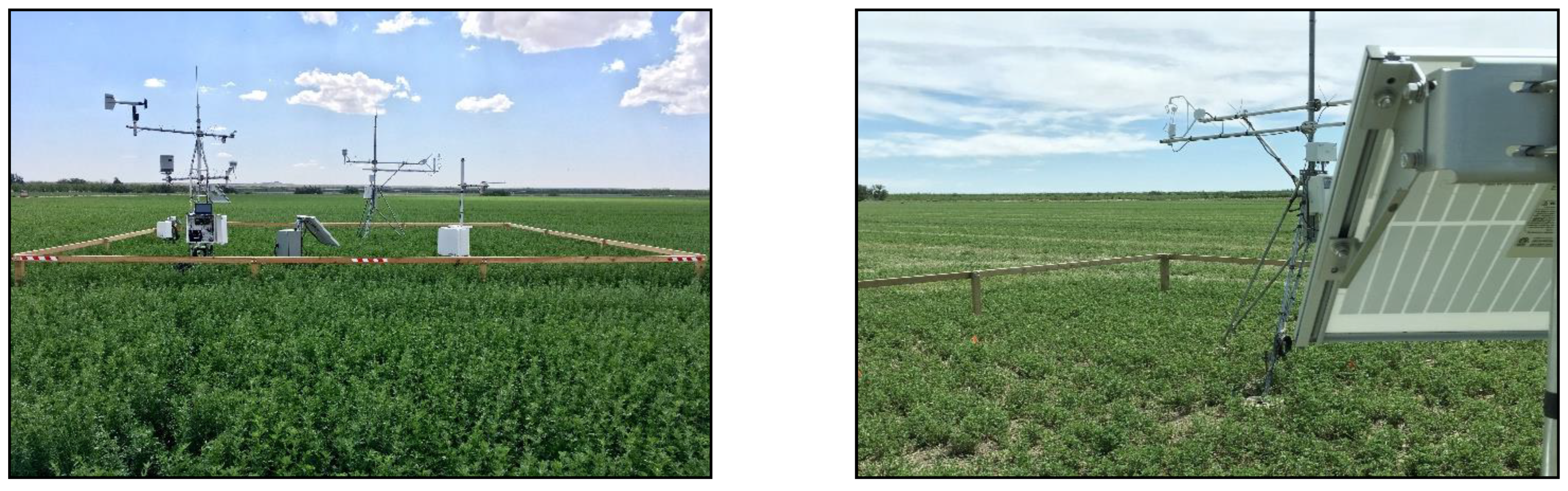
2.3. ET Measurement Using Eddy Covariance

The evapotranspiration of alfalfa was determined by measuring the components of the energy budget (net radiation, soil heat, latent, and sensible heat fluxes) to determine the ET of alfalfa. The sensible heat and latent heat fluxes were measured using the eddy covariance technique. The measurements and instrumentation used to determine the actual ET in this study are described in Boyko et al. [4], a study of Willie’s Farm to determine groundwater recharge in 2017. The eddy covariance instrumentation “system” was set near the center of the field, denoted as a white circle in Figure 1. The location of the eddy covariance system was selected to ensure adequate fetch distance to the edge of the field in order for the eddy covariance sensors (CSAT3 sonic anemometer and water vapor Open Path LICOR 7500 by Campbell Scientific Inc., Logan, UT, USA) to measure the relative contribution of sensible and latent heat (LE) fluxes from the alfalfa field. The system was set inside a wooden fence placed in such a way as to avoid air movement and minimize interference with or obstruction of the sensors (Figure 2). The components of the energy budget, including net radiation and sensible and soil heat fluxes, were measured every 30 min, and latent heat flux was determined as a residual. The 30 min data were totaled to obtain daily LE values (24 h), which were then converted to the daily equivalent depth of water as the ET in mm.

2.4. Reference Evapotranspiration

Evapotranspiration referenced to grass (ETo) was calculated using weather data measured at the Leyendecker III weather station. The station was located about 1 km from Willie’s Farm at 32°12′3.26″N and 106°44′34.00″W, with an elevation of 1176 m AMSL (white triangle, Figure 1). The weather data included maximum and minimum air temperature and relative humidity, average wind speed, and solar radiation. The Leyendecker III weather station instrumentation is described in Boyko et al. [4]. The ETo was calculated using the ASCE-EWRI standardized Equation (1) [39] for short crops (i.e., grass). The ETo during the satellite overpass was calculated using hourly weather data measured by the station and Equation (1). Daily ETo was then determined from the summation of hourly ETo values.

$$\mathrm{ETo}=\frac{0.408\left({\mathrm{R}}_{\mathrm{n}}-\mathrm{G}\right)+\mathsf{\gamma }\frac{{\mathrm{C}}_{\mathrm{n}}}{\mathrm{T}+273}{\mathrm{u}}_2\left({\mathrm{e}}_{\mathrm{s}}-{\mathrm{e}}_{\mathrm{a}}\right)}{∆+\mathsf{\gamma }\left(1+{\mathrm{C}}_{\mathrm{d}}·{\mathrm{u}}_2\right)}$$

(1)

where ETo is hourly evapotranspiration (mm/h) referenced to grass, Rn is net radiation (MJ/m²/h), G is the soil heat flux (MJ/m²/h), T is the mean hourly air temperature (°C) at 1.5 to 2.5 m height, u₂ is the mean hourly wind speed (m/s) at 2 m height, e_s is the saturated vapor pressure (kPa), e_a is mean actual vapor pressure (kPa), ∆ is the slope of the saturated vapor pressure–air temperature curve (kPa/°C), and γ is psychrometric constant (kPa/°C). C_n and C_d are coefficients, where C_n is equal to 37 (K∙mm∙s³/Mg/h) during daytime and nighttime and C_d is equal to 0.24 (s/m) during the daytime and 0.96 (s/m) during the nighttime. The detailed calculation of ETo is described in ASCE-EWRI [39].

2.5. Satellite Images and Preprocessing

Landsat-8 images for the study site from 2017 for path 33 and row 38 were acquired for clear-sky conditions (cloud cover ranging from 0 to 1%) from the USGS Earth Explorer website [36]. Eight images of clear-sky days were acquired in 2017 (

Table 1. The dates and path/row image scenes of the Landsat-8 satellite’s Operational Land Imager (OLI) and the Thermal Infrared Sensor (TIRS) times (Coordinated Universal Time or UTC) of the overpass.

Dates	Path/Row	UTC	Satellite	Sensors
25 Febraury 2017	33/38	17:39:34	Landsat-8	OLI/TIR
13 March 2017	33/38	17:39:25	Landsat-8	OLI/TIR
30 April 2017	33/38	17:38:58	Landsat-8	OLI/TIR
17 June 2017	33/38	17:39:24	Landsat-8	OLI/TIR
5 September 2017	33/38	17:39:47	Landsat-8	OLI/TIR
7 October 2017	33/38	17:39:57	Landsat-8	OLI/TIR
23 October 2017	33/38	17:39:59	Landsat-8	OLI/TIR
24 November 2017	33/38	17:39:52	Landsat-8	OLI/TIR

). The images, stored in the Level-1 GeoTIFF data format, were projected onto the Universal Transverse Mercator (UTM) coordinate system and the WGS 1984-Zone 13N Datum. The Landsat-8 satellite has two sensors: the Operational Land Imager (OLI) and the Thermal Infrared Sensor (TIRS). The visible and near-infrared (NIR) bands have a spatial resolution of 30 m × 30 m and a temporal resolution of 16 days (16 days between the images). The digital numbers of Landsat-8 images were calibrated for either reflectance or radiance using the Environment for Visualizing Images (ENVI version 5.5 by L3Harris Geospatial Co., Boulder, CO, USA) program. Reflectance bands 1 to 7 were used to determine agronomic parameters such as vegetation indices and albedo, whereas thermal band 10 was used to calculate the land surface temperature (LST). Band number 10, of 30 m resolution, was converted to radiance and then from the spectral radiance to brightness temperature using the ENVI 5.5^® program. Then, emissivity-corrected LSTs (Equation (2)) were calculated following Artis and Carnahan [40].

$$\mathrm{LST}=\frac{{\mathrm{T}}_{\mathrm{B}}}{1+\left(\frac{\mathsf{\lambda }\times {\mathrm{T}}_{\mathrm{B}}}{\mathsf{\rho }}\right)\ln \left(\mathsf{\epsilon }\right)}$$

(2)

where T_B is the effective at-sensor (at satellite) brightness temperature (K); λ is the wavelength of emitted radiance (m; λ = 11.5 µm) [41]; ε is the land surface (according to the nature of land cover) emissivity [42]; and $\rho$ is the spectral density of electromagnetic radiation (1.438 × 10⁻² mK) calculated using Planck’s black-body equation, ρ = (h∙c)/σ, where h is Plank’s constant (6.626 × 10⁻³⁴ J∙s), c is the speed of light (2.998 × 10⁸ m/s), and σ is the Boltzmann constant (1.381 × 10⁻²³ J/K).

Atmospheric corrections were applied to the Landsat-8 images using the Fast Line-of-sight Atmospheric Analysis of Spectral Hypercubes (FLAASH) tool in ENVI 5.5^® to minimize the impact of the atmosphere on ground-reflected radiation. This correction process necessitated ancillary data input, including latitude, longitude, flight date and time, sensor altitude and ground elevation, pixel size, and initial ground visibility. The preprocessed Landsat-8 images for the year 2017 and the respective Coordinated Universal Time (UTC) of the scene overpass and satellite sensors are listed in Table 1.

2.6. Remote Sensing ET Models

Two models, the mapping evapotranspiration at high resolution with internalized calibration (METRIC) and operational simplified surface energy balance (SSEBop), were used in this study to determine the ET of alfalfa. The METRIC model was developed by Allen et al. [9,10] and the SSEBop model by Senay et al. [15]. The following sections describe the two models.

2.6.1. METRIC Model

The METRIC model, introduced by Allen et al. [9,10] in Kimberly, Idaho, underwent a comparative analysis with the “ground truth” measurements derived from lysimeter observations as per Wright’s [43] study. METRIC, a refined version of the surface energy balance algorithms for land (SEBAL) model [13,14], utilizes identical algorithms and computational frameworks [9]. METRIC is a surface energy balance method that uses remotely sensed surface reflectance, near-infrared (NIR), and thermal bands (IR) to estimate the latent heat flux as a “residual” of the land surface energy balance (Equation (3)); the latent heat flux is then converted to ET.

$${\mathrm{LE}}_{\mathrm{inst}}={\mathrm{R}}_{\mathrm{n}}-\mathrm{G}-\mathrm{H}$$

(3)

where LE_inst is the instantaneous latent heat flux (W/m²). The LE_inst can then be expressed in terms of water depth per unit area (mm/h) or instantaneous evapotranspiration (ET_inst). The ET_inst in the models is calculated by multiplying LE_inst by 3600 s/h (converts seconds to hours) and dividing it by the latent heat of vaporization of water, which is a function of temperature (the value is about 2.45 MJ/kg at 20 °C), and the density of water (~1000 kg/m³). R_n is the net radiation (W m⁻²), G is the soil heat flux (W/m²), and H is the sensible heat flux (W/m²). The R_n in the METRIC model is calculated from the satellite-measured narrow-band reflectance and surface temperature as the difference between all incoming and outgoing short- and long-wave radiations [10]. The soil heat flux (G) is estimated from R_n using an empirical equation [9,10] based on vegetation cover, surface temperature, and albedo. The sensible heat flux (H) is calculated using the bulk aerodynamic resistance function (r_ah) and near-surface temperature gradient (dT) through an iterative process considering the effects of atmospheric stability. The dT is calculated using a simple linear function between two near-surface heights, $z_1$ and $z_2$, generally 0.1 and 2 m, using wind speed extrapolated to some blending height above the ground surface of 200 m [9,10,11].

METRIC utilizes an auto-calibration method using the ground-based calculated hourly ET (ETr), where ETr is evapotranspiration of the standardized 0.5 m tall alfalfa reference crop surface. The daily ET (or ET₂₄), which is more useful in irrigation management practices, is calculated using the crop evapotranspiration fraction (ET_f) as a ratio of ET_inst from each pixel to ETr calculated from weather data at the time of the satellite overpass image (ET_f = ETinst/ETr). The computed ET_f at the image time is assumed to be constant over 24 h as a time-based transfer mechanism for most crops that have developed to maximize photosynthesis [9]. The use of ETr during 24 h tends to capture the advective effects of the changing weather conditions during the day on ET [9,10].

In this study, the reference ET for well-watered grass (ETo) instead of the ETr was utilized for internal calibration and for estimating ET₂₄ following Chavez et al. [44] and He et al. [45]. The daily actual evapotranspiration (ET₂₄) in mm/day for each pixel was then calculated using Equation (4) by multiplying the daily ET_f with the daily standardized 0.12 m well-watered grass reference (ET_o24).

$${\mathrm{ET}}_{24}={\mathrm{ET}}_{\mathrm{f}}\times {\mathrm{ET}}_{\mathrm{o}24}$$

(4)

2.6.2. SSEBop Model

The SSEBop model introduces a parameterization where the difference between the hot and cold reference values is predefined for a given pixel [15]. SSEBop is distinct from existing remote sensing models like SSEB [46], SEBAL [13,14], or METRIC [9,10], which use a set of reference hot and cold pixel pairs. The SSEBop model is closely aligned with the SEBS model by Su [16], which determines the evaporative fraction based on the energy balance of each pixel at the wet and dry limiting conditions, where actual ET occurs between these two limits. This approach is designed to derive energy balance components in situations with limited wet and dry pixels. Notably, this model requires fewer parameters compared to other models and integrates remote sensing data with ground measurements to estimate ETa [15]. Unlike other models, SSEBop does not calculate latent heat flux as a residual in the energy balance because it does not attempt to solve all energy balance components. In the SSEBop model, ETa is directly computed using Equation (5), where the evapotranspiration fraction (ET_f) is multiplied by the daily grass reference ET (ET_o) and a scaling coefficient, k (–). The scaling factor of 1.2 is recommended for scaling ET_o into a level of maximum ET experienced by an aerodynamically rougher crop or calibrated for the study area. The k value was considered 1 in this study and is dropped out of the equations. The ET_f is calculated under limited conditions of wet and dry pixels using Equation (6).

$${\mathrm{ET}}_{\mathrm{a}}={\mathrm{ET}}_{\mathrm{f}}\times {\mathrm{k}\times \mathrm{ET}}_{\mathrm{o}}$$

(5)

$${\mathrm{ET}}_{\mathrm{f}}=\frac{{\mathrm{T}}_{\mathrm{h}}-{\mathrm{T}}_{\mathrm{s}}}{{\mathrm{T}}_{\mathrm{h}}-{\mathrm{T}}_{\mathrm{c}}}$$

(6)

where T_s is the land surface temperature of the pixel observed by the satellite, T_h is the estimated T_s at the idealized reference “hot” condition of the pixel, and T_c is the estimated T_s at the idealized reference “cold” condition of the pixel. The difference between T_h and T_c is the dT. The SSEBop estimates T_c from the near-surface daily maximum air temperature using a correction factor, and T_h is then calculated as the sum of T_c and dT. See Senay et al. [15] for a further explanation on estimating the T_s and T_c and the related assumptions.

The dT is computed based on the assumption that daily latent heat flux for dry, bare soil is equal to zero, and sensible heat flux is at a maximum. Since the G and LE are considered zero, the R_n equals H in the energy balance (Equation (3)) and can be calculated using Equation (7). All net radiation is assumed to be consumed as sensible heat flux at hot boundary conditions. For a clear-sky day, R_n (W/m²) received at an idealized bare and dry surface of a pixel is calculated by using a series of equations, as detailed in Allen et al. [8] and iterated by Senay [15]. Therefore, H (W/m²) is approximated (R_n = H), and hence dT (K) is calculated by rearranging Equation (7).

$${\mathrm{R}}_{\mathrm{n}}=\mathrm{H}=\frac{{\mathsf{\rho }}_{\mathrm{a}}\times {\mathrm{c}}_{\mathrm{p}}\times \mathrm{dT}}{{\mathrm{r}}_{\mathrm{ah}}}$$

(7)

where ρ_a is air density (kg/m³), c_p is the specific heat of moist air at constant pressure (~1013 J/kg/K), and r_ah is the aerodynamic resistance for heat (s/m). A constant value of $r_{ah}$ equal to 110 (s/m) is used in the SSEBop model [15]. Daily ETa in mm/day is then calculated:

$${\mathrm{E}\mathrm{T}}_{\mathrm{a}}=\frac{{\mathsf{\rho }}_{\mathrm{a}}\times {\mathrm{c}}_{\mathrm{p}}\times ({\mathrm{T}}_{\mathrm{h}}-{\mathrm{T}}_{\mathrm{S}})}{{\mathrm{R}}_{\mathrm{n}}\times {\mathrm{r}}_{\mathrm{ah}}}\times {\mathrm{ET}}_{\mathrm{o}}$$

(8)

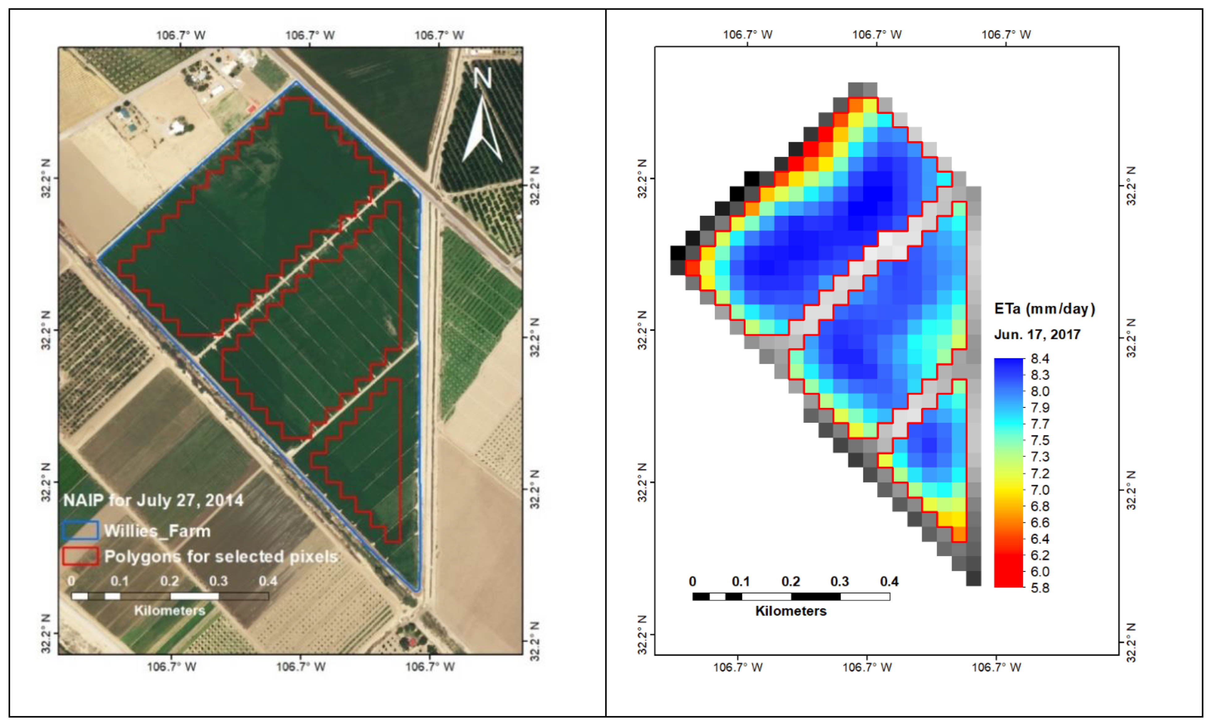
2.7. Pixel Selection

The resolution of each pixel from Landsat-8 is 30 m by 30 m. The pixels representing the alfalfa were selected to avoid the pixels on the edge of the plots affected by local advection, such as the roads and canals that are of different surface conditions. Removing the “contaminated” pixels reduces the errors introduced by the models for those pixel conditions when compared to ground-level eddy covariance ET measurements. A polygon is created to select pixels in each satellite ET image scene of the alfalfa fields by overlaying an aerial image from the NAIP with the same polygon on the satellite model image of ET. An example of an aerial image (left image) of Willie’s overlaid on METRIC ET estimates for 17 June 2017 (right image) is shown in Figure 3; one to two contaminated pixels from the field boundary were removed from the image scenes. From a total of 395 pixels, 273 pixels were used in the ET analysis.

2.8. Statistical Analysis

The estimated ETa values derived from the METRIC and SSEBop models for the clear-sky image during the satellite overpass at the study site were compared with the eddy covariance measurements of ET using linear regression. The eddy covariance ETa was considered the independent variable, and the remote sensing model ET was considered the dependent variable. The statistical indicators considered included the coefficient of determination (R²), standard error of estimate (SEE) of the predicted y-dependent value for each x-independent in the regression, and mean relative difference (MRD). The daily average ETa values of the selected pixels, as explained in Section 2.7 for METRIC and SSEBop, during the days of clear-sky overpass (Table 1) were also compared using a linear regression.

3. Results and Discussion

3.1. Weather

The distribution of daily climate data for 2017 at Leyendecker III weather station is illustrated in Figure 4. From weather measurements at the Leyendecker III climate station in 2017, the mean daily temperatures varied from 6.4 °C to 27.2 °C with an average of 17.05 °C. Temperatures of 38 °C and higher were observed for about two weeks from 15 June to 4 July, with the highest temperature of 42.44 °C recorded on June 23rd. The lowest temperature of −9.28 °C was recorded on December 8th. It is typical for the region to experience high temperatures (>35 °C) in June and July and sometimes in August as well. The daily mean relative humidity varied from 22% to 81%, averaging 49.9%. High humidity was observed in the early mornings, and low humidity was observed in the late afternoons. The recorded annual precipitation was 279 mm, which was higher than the annual average of 222 mm reported by Malm [38]. July received the highest total precipitation of 111 mm, followed by 85 mm in August, which equates to 70% of the total annual precipitation. Less than 12 mm per month of rainfall was received from February through June and from October through December. Due to the low amount of precipitation, the farmers in the region rely on irrigation using either groundwater or surface water from the Rio Grande. The mean daily wind speeds ranged from 0.56 m/s to 5.27 m/s, with an average of 1.64 m/s. The daily solar radiation recorded in 2017 ranged from 3.8 MJ/m² to 32.34 MJ/m² with an annual average of 21 MJ/m².

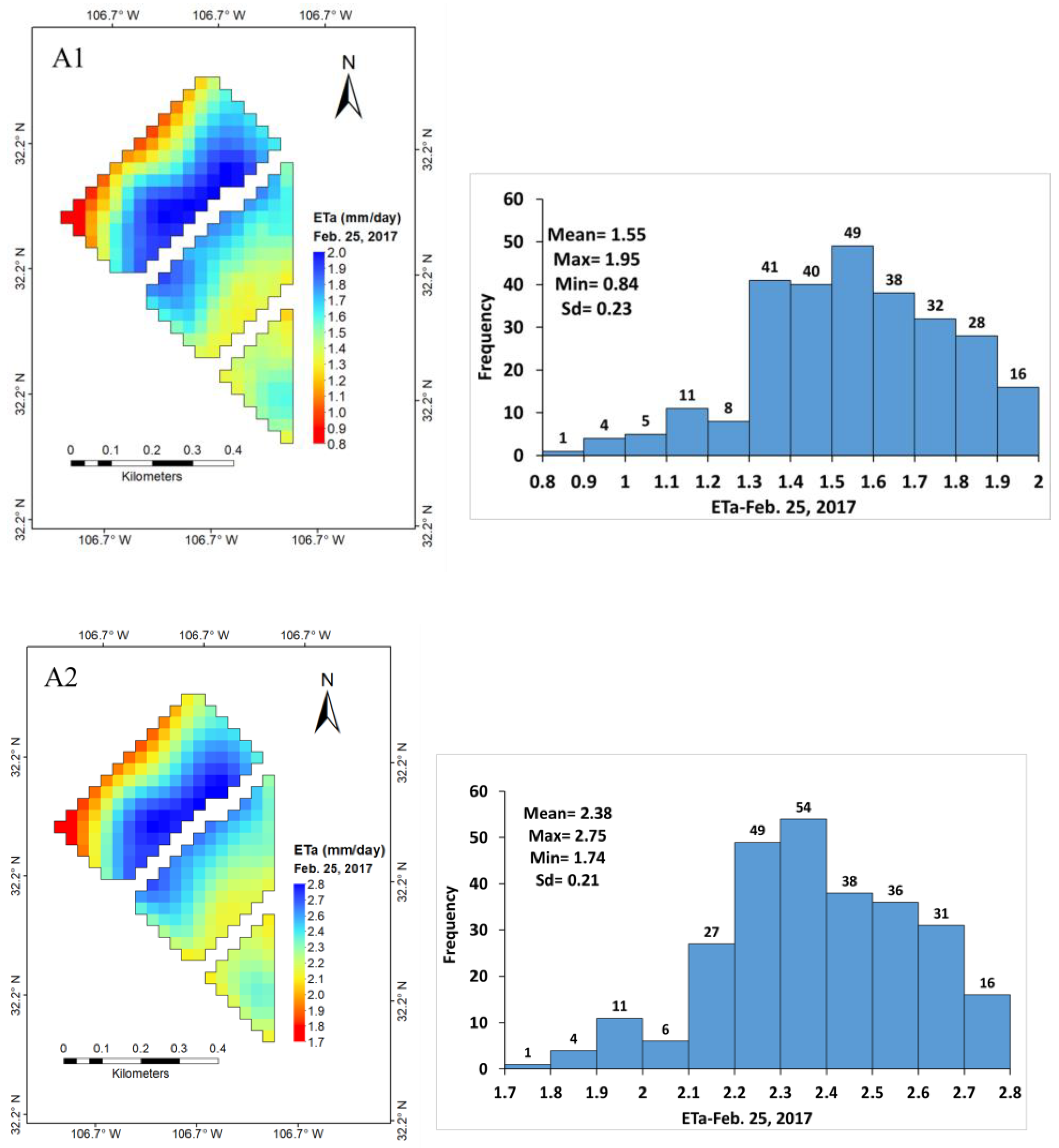
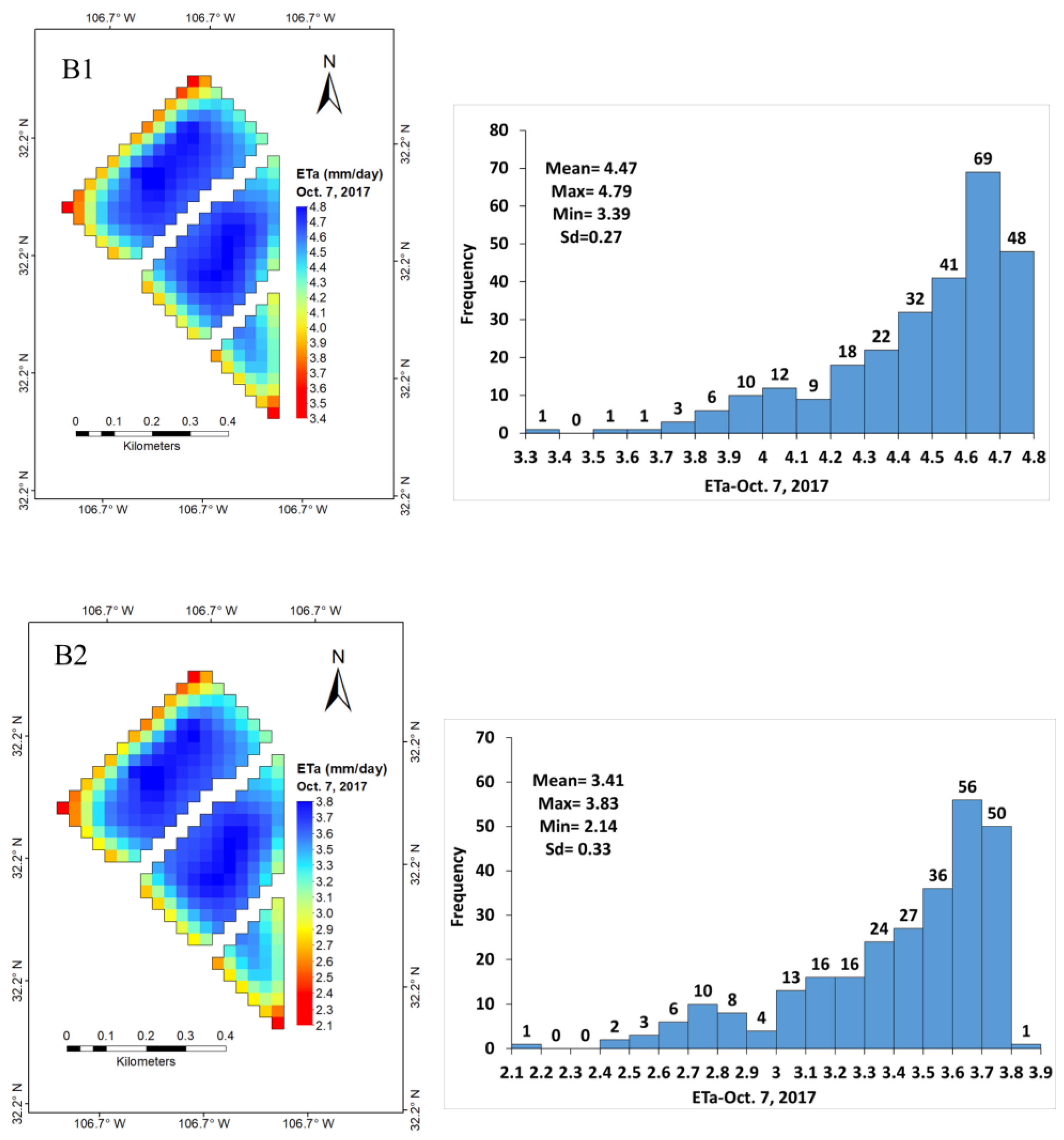
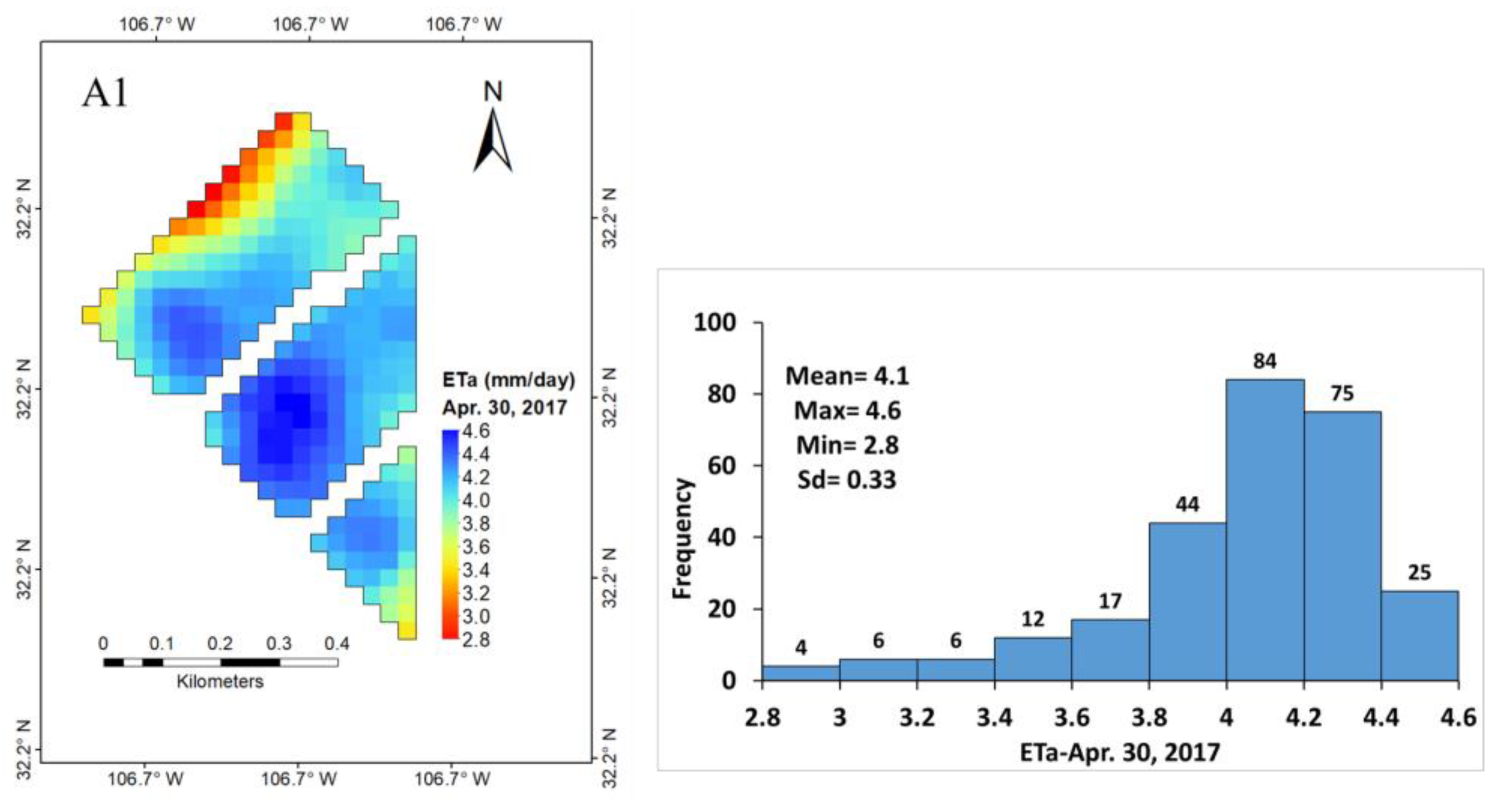
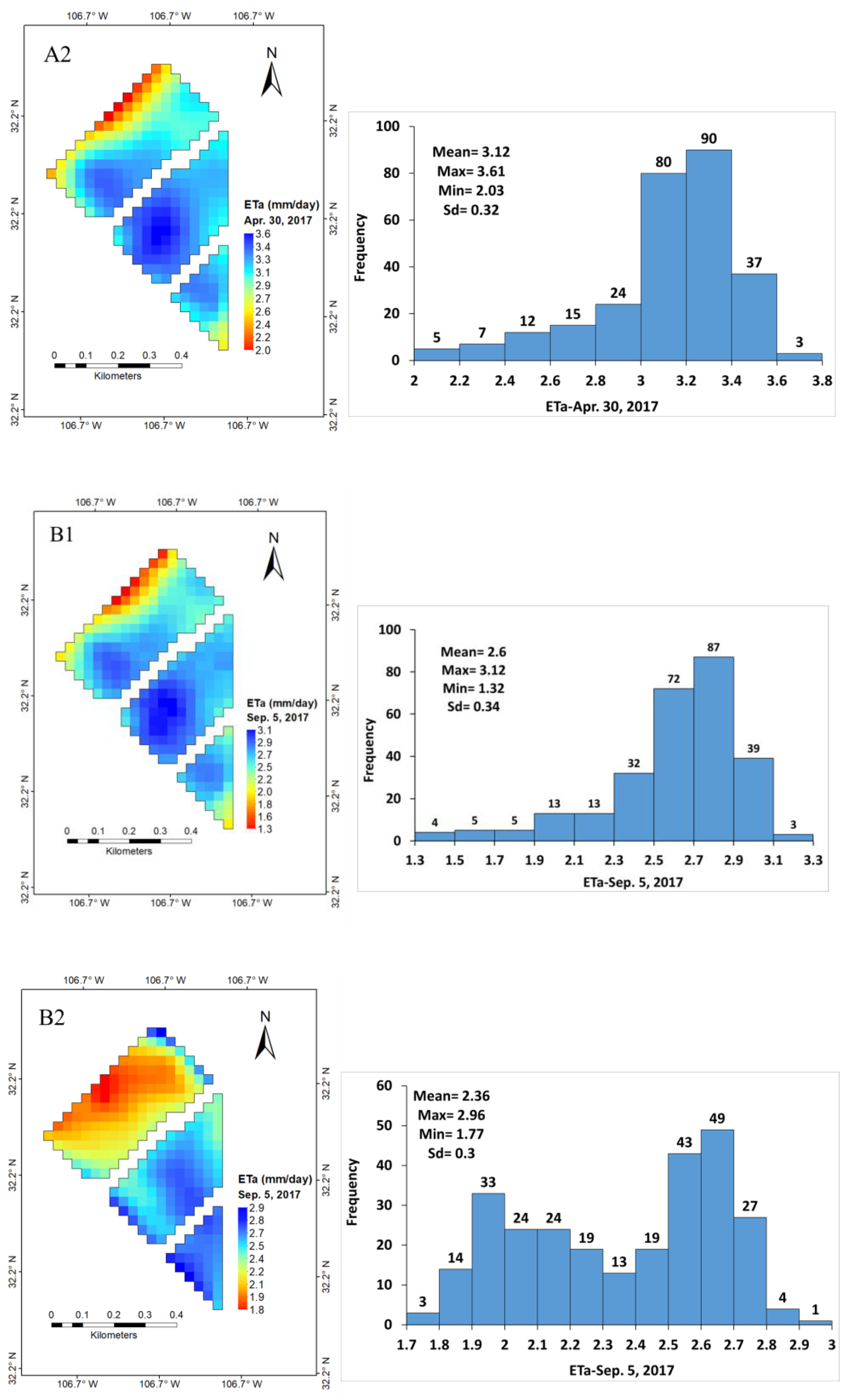
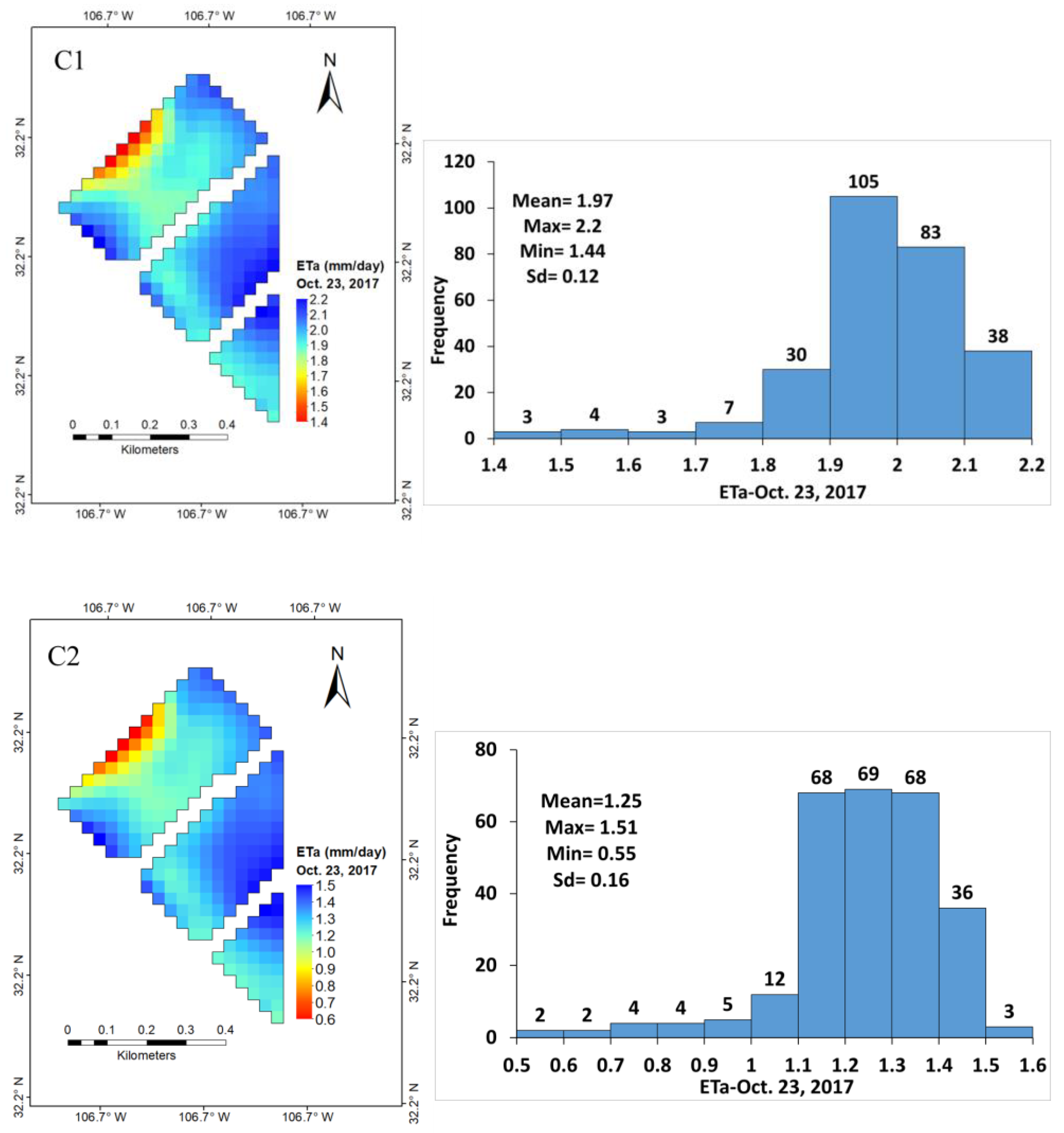
3.2. Spatial Distribution of ET

After filtering the “contaminated” pixels, 273 pixels (30 m × 30 m each) were considered representative of alfalfa. The ETa of alfalfa from the METRIC and SSEBop models varied on a spatial and temporal scale within each field. The ETa for each pixel using the two models and their respective ETa histograms during the beginning of the growing season in February and March and at the final growth stage in November are shown in Figure 5. Similarly, the ETa distribution of alfalfa using the two models for June and October and their respective histograms when the plants are at full growth are shown in Figure 6, and that for when the alfalfa was harvested (cut) is shown in Figure 7. The spatial distribution of ETa within the fields near the irrigation canal had a good start on growth, as reflected by higher ETa values (darker blue color pixels) in February and March (Figure 5). As the season progressed and the weather started to warm, those plants away from the irrigation canal started to transpire more, as reflected in the ETa values of the pixels that increased inwards toward the southeast and northwest directions within the field plots (Figure 6). The ranges of ETa values estimated by METRIC, SSEBop, and ETo are presented in

Table 2. Evapotranspiration (ET) was estimated by METRIC, SSEBop, and eddy covariance and referenced to grass (ETo). Values in the parenthesis are mean ET.

Landsat-8 Dates	METRIC (mm)	SSEBop (mm)	Eddy Cov. (mm)	ETo (mm)
25 Febraury 2017	0.84–1.95 (1.55)	1.74–2.75 (2.38)	1.79	3.64
13 March 2017	2.49–4.16 (3.65)	2.03–3.88 (3.28)	3.84	4.79
30 April 2017 *	2.83–4.55 (4.05)	2.03–3.61 (3.12)	4.81	5.80
17 June 2017	5.87–8.45 (7.80)	4.54–7.28 (6.53)	6.75	6.78
5 September 2017 *	1.34–3.12 (2.60)	1.77–2.96 (2.36)	2.98	6.17
7 October 2017	3.39–4.79 (4.47)	2.14–3.83 (3.41)	4.51	3.96
23 October 2017 *	1.44–2.20 (1.97)	0.55–1.51 (1.25)	1.53	3.58
24 November 2017	1.72–2.68 (2.40)	0.69–2.21 (1.86)	2.18	2.19

* Harvesting periods; ETo calculated from hourly data measured at the Leyendecker III weather station.

. The full-grown alfalfa daily ETa for 17 June for 273 pixels as determined by METRIC ranged from 5.87 to 8.45 mm with an average of 7.80 mm (std. dev. 0.48 mm), and that for SSEBop ranged from 4.54 to 7.28 mm with an average of 6.53 mm (std. dev. 0.59 mm). Both models showed a decline in ETa during the harvesting periods, as would be expected since the plants do not have leaves and transpire less. Alfalfa recovered quickly after harvesting, as reflected in the rise in ETa. The eddy covariance daily ETa and the daily calculated ETo (referenced to grass, ETz [4]) values and harvesting days are presented in Boyko et al. [4] Figure 2.

It is difficult to separate soil moisture deficiency on a farm from the stages of plant growth, especially at the beginning of the season, unless soil moisture at different depths is measured in several locations of the fields. This procedure, however, can be expensive and time consuming. In a related study of Willie’s Farm to determine groundwater recharge [4], the soil moisture profile at depths of 30 cm, 60 cm, 90 cm, and 120 cm was measured near the middle of the farm using volumetric water content reflectometers (VWC Model CS 616 by Campbell Scientific, Logan, UT, USA). The measured daily soil moisture values are presented in Boyko et al. [4] Figure 3. The irrigation and the effective precipitation events were reflected in the soil moisture profile measurements; the soil moisture increased during irrigation and high precipitation.

The METRIC and SSEBop models captured the variability in ETa reflecting plant transpiration. They captured the status of soil moisture, which increased inward toward the southeast and northwest directions from the field’s border with the irrigation canal outlets. This variability explains the lack of soil moisture at the beginning of the growing season in some areas of the field in January and February. In February and March, rainfall of less than 10 mm per month was received, and the alfalfa fields were not irrigated until March 3. The limited amount of soil moisture near the irrigation canals was from the previous year of late-season irrigation. In January and February, the top soils, sampled by hand and visual inspection, away from the canal were drier than those near the canal outlets. The remote sensing spatial distribution of ET estimates by METRIC and SSEBop showed similar patterns even though the values by the two models were slightly different. They both implicitly reflected the farm’s plant conditions, soil moisture, and irrigation conditions.

The plants adjacent to the concrete-lined irrigation canal outlets had access to more soil moisture than those away from the canal during the early part of the season. This soil condition was probably due to inefficient water distribution. This condition was noticed early during the season when the fields were irrigated with groundwater. The irrigation well and the pump were not producing enough water to raise the pressure head in the canal for full outlet flows. The flows in the concrete canal using groundwater ranged from 0.12 to 0.16 m³/s, and the amount of each irrigation varied from 134 mm to 222 mm [4]. As a result, the time it took for the water to reach the end of the fields and replenish water quickly in the root zone was reduced. Even though the field was laser leveled in 2014 before the alfalfa was seeded, the on-field irrigation efficiency was low. A total of 994 mm was applied during the six irrigation events using groundwater from March through June, and from July through November, 880 mm was applied during the five irrigation events using surface water from the Rio Grande. It is more likely that the soils near the irrigation outlets received more water during winter, which penetrated deeper and remained in storage rather than at the edge of the fields. This condition, however, did not last long as the season progressed. The soil moisture was replenished faster when the Rio Grande water was available for irrigation. The diversion of the water from the main irrigation distribution canal, managed by Elephant Butte Irrigation District, near the farm, allowed for higher flow and head in the canal and therefore improved canal efficiency and on-field irrigation uniformity. On-farm irrigation efficiency for Willie’s Farm was determined by Boyko et al. [4] as 59.93%.

It can be seen that in November (Figure 5), despite the end of the season, the majority of the plants in each pixel are transpiring uniformly; see the histogram of ETa for each pixel. The uniform transpiration shown by the pixel distribution is due to 11 irrigation applications, which kept the soil moist up to a depth of about 1.2 m. During the growing season, the plants developed to full growth and became lush, as reflected in high and spatially distributed ETa values in the field during June and October (Figure 6). The METRIC and SSEBop models were able to reflect the harvesting periods in April, September, and October well (Figure 7). These models, despite their differences in ET values, have reflected different stages of alfalfa growth and harvesting days, as well as soil moisture distribution due to irrigation issues. The spatial variability in ETa in each field during the period of harvesting is also reflected in the images.

This study shows that high-resolution spatiotemporal satellite-derived ETa maps using models such as METRIC and SSEBop can be valuable in diagnosing issues that can help the farmer and water managers in decision-making to improve water conservation and crop yield at a farm scale. One of the major advantages of using remote sensing-based ET estimation when compared to ground-point and one-number integrated value (e.g., eddy covariance and Bowen ratio) measurements is that it provides the spatiotemporal variability of ET. Despite the current anecdotal availability of clear-sky images that are spaced several days apart and of limited resolution, the satellite-based methods for estimating the ETa of crops can provide information that could be used to improve on-farm irrigation application efficiency, conserve water and soil nutrients, manage salinity, and ensure crop yield. This study shows that spatiotemporal variabilities in crop ETa estimates using remote sensing-based ET models such as METRIC and SSEBop can provide valuable information for improving farming practices. This study, however, did not have the opportunity to study the ET of alfalfa after the farmer made changes to improve the irrigation conveyance canal and on-farm irrigation.

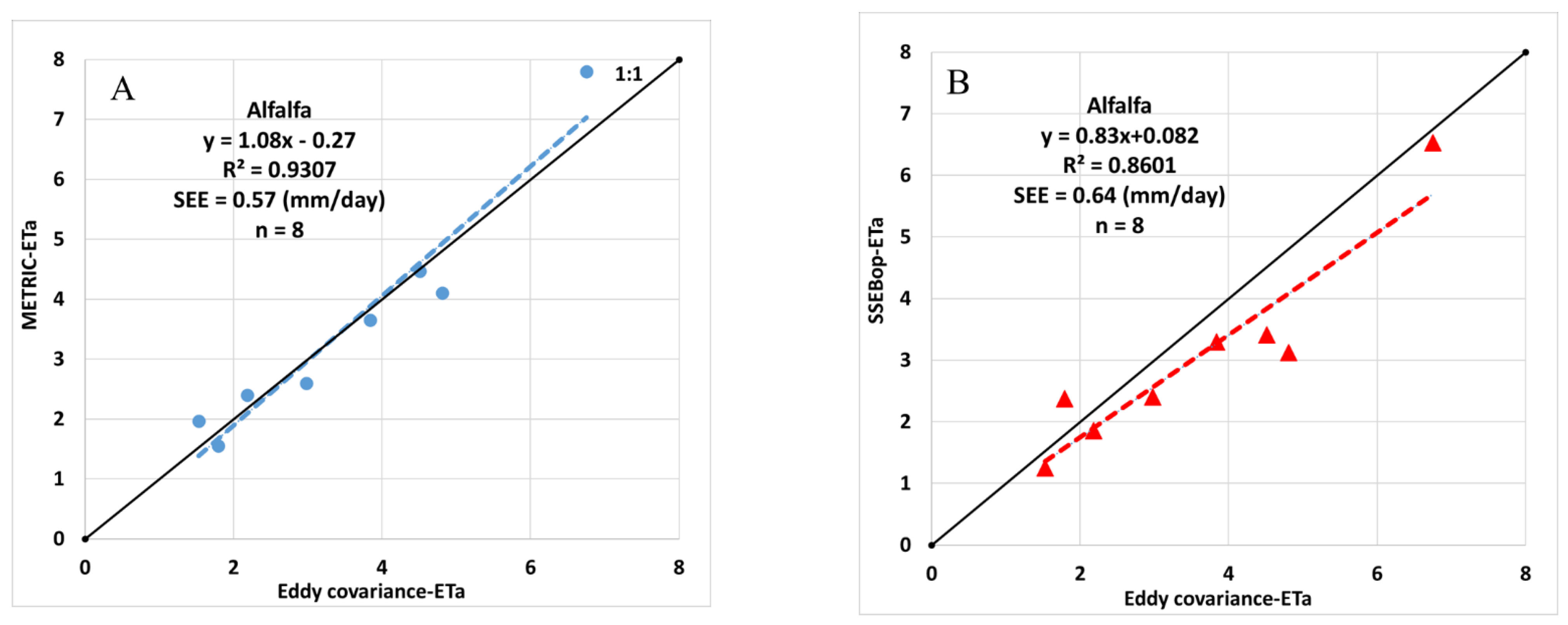
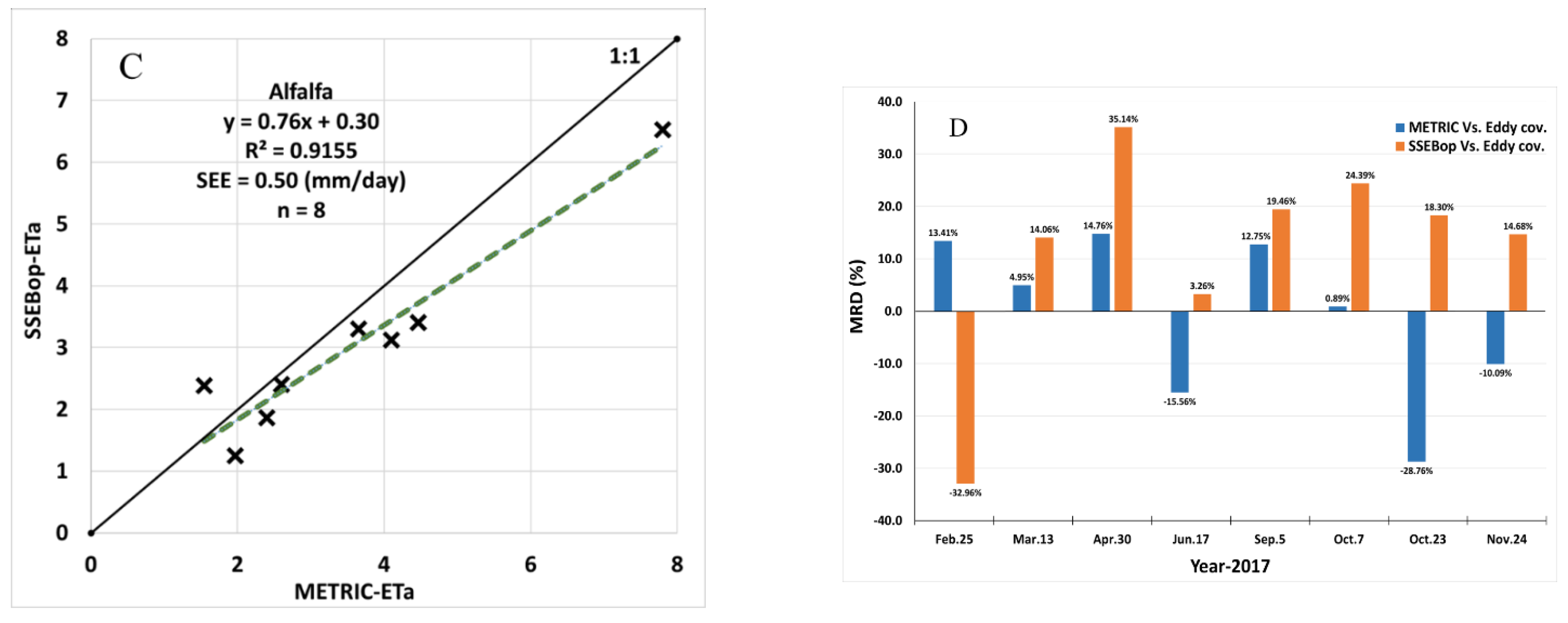
3.3. Comparison of ET Estimates

The estimates of the daily ETa of alfalfa by METRIC, SSEBop, and the eddy covariance method were compared using a simple linear regression for 2017. Refer to Boyko et al. [4] for a detailed explanation of the eddy covariance data, respective required correction methods, fetch distances, and energy closure for this study. Eight days of “good” satellite images were available for the study site (Table 1). Overall, the ETa of alfalfa by the two models correlated well with eddy covariance ETa estimates during the full growth and harvesting periods. The linear regression comparison is shown in Figure 8. The METRIC model ETa compared more closely (R² = 0.9307, SEE = 0.57 mm/day, n = 8 days) to eddy covariance than the SSEBop model (R² = 0.8601, SEE = 0.64 mm/day, n = 8 days). Comparison between the two models (METRIC vs. SSEBop) using simple regression shows a slope of 0.76 and an intercept of 0.30 mm/day with a SEE of 0.50 mm/day. The coefficient of determination value indicates that the variability in the METRIC ETa can explain 91.55% of the variability in SSEBop ETa estimates. The largest percentage mean relative differences (MRDz) between the two models and eddy covariance ETa were observed when the soil was dry and when alfalfa was harvested (Figure 8D). It is a common practice by the farmers to allow the fields to dry for easy access by the baler machinery before and during the harvesting period. After harvesting, the fields are irrigated immediately to allow the plants to grow back quickly.

4. Conclusions

METRIC and SSEBop models were used to estimate the ETa of Willie’s alfalfa farm in the Mesilla Valley of New Mexico, USA, in 2017 using Landsat 8 satellite data. Images of ETa using the models for the fields were created for eight days of clear-sky satellite data spread throughout the growing season. The images reflected the days of early stages of alfalfa growth, full growth, and harvesting periods. The integrated ETa values estimated by the models were compared to estimated ETa by on-the-ground measurements using the eddy covariance method and each other. The comparison showed that 91.55% of the variability in SSEBop ETa estimates can be explained by the variability in the METRIC ETa estimates, and the variability in eddy covariance ETa can explain 93.07% of the variability in METRIC ETa and 86.01% in SSEBop. This study showed that spatiotemporal variabilities in crop ET estimates using remote sensing-based ET models such as METRIC and SSEBop can provide valuable information to farmers for decision-making to improve irrigation management and farming practices.

References

1. US Department of Agriculture–National Agricultural Statistics Service (NASS) New Mexico Field Office. 2018 New Mexico Agricultural Statistics; USDA, National Agricultural Statistics Service: Washington, DC, USA, 2018. Available online: https://www.nass.usda.gov/Statistics_by_State/New_Mexico/Publications/Annual_Statistical_Bulletin/2018/2018-NM-Ag-Statistics.pdf (accessed on 20 March 2022).
2. Lacefield, G.; Ball, D.; Hancock, D.; Andrae, J.; Smith, R. Growing Alfalfa in the South; National Alfalfa and Forage Alliance: Saint Paul, MN, USA, 2009. [Google Scholar]
3. Sammis, T.W. Yield of Alfalfa and Cotton as Influenced by Irrigation 1. Agron. J. 1981, 73, 323–329. [Google Scholar] [CrossRef]
4. Boyko, K.; Fernald, A.G.; Bawazir, A.S. Improving groundwater recharge estimates in alfalfa fields of New Mexico with actual evapotranspiration measurements. Agric. Water Manag. 2021, 244, 106532. [Google Scholar] [CrossRef]
5. Wright, J.L. Daily and Seasonal Evapotranspiration and Yield of Irrigated Alfalfa in Southern Idaho. Agron. J. 1988, 80, 662–669. [Google Scholar] [CrossRef]
6. Wagle, P.; Gowda, P.H.; Northup, B.K. Dynamics of Evapotranspiration over a Non-Irrigated Alfalfa Field in the Southern Great Plains of the United States. Agric. Water Manag. 2019, 223, 105727. [Google Scholar] [CrossRef]
7. Djaman, K.; Koudahe, K.; Mohammed, A.T. Dynamics of Crop Evapotranspiration of Four Major Crops on a Large Commercial Farm: Case of the Navajo Agricultural Products Industry, New Mexico, USA. Agronomy 2022, 12, 2629. [Google Scholar] [CrossRef]
8. Allen, R.B.; Pereira, L.S.; Raes, D.; Smith, M.S. Crop evapotranspiration (guidelines for computing crop water requirements). In FAO Irrigation and Drainage Paper 56; Food and Agriculture Organization of the United Nations: Rome, Italy, 1998; Volume 56, p. 300. [Google Scholar]
9. Allen, R.G.; Tasumi, M.; Trezza, R. Satellite-Based Energy Balance for Mapping Evapotranspiration with Internalized Calibration (METRIC)—Model. J. Irrig. Drain. Eng. 2007, 133, 380–394. [Google Scholar] [CrossRef]
10. Allen, R.G.; Tasumi, M.; Morse, A.; Trezza, R.; Wright, J.L.; Bastiaanssen, W.; Kramber, W.; Lorite, I.; Robison, C.W. Satellite-Based Energy Balance for Mapping Evapotranspiration with Internalized Calibration (METRIC)—Applications. J. Irrig. Drain. Eng. 2007, 133, 395–406. [Google Scholar] [CrossRef]
11. Allen, R.G.; Tasumi, M.; Trezza, R.; Robison, C.W.; Garcia, M.; Toll, D.; Arsenault, K.; Hendrickx, J.M.H.; Kjaersgaard, J. Comparison of Evapotranspiration Images Derived from MODIS and Landsat Along the Middle Rio Grande. In Proceedings of the World Environmental and Water Resources Congress 2008: Ahupua’A, Honolulu, HI, USA, 12–16 May 2008; pp. 1–13. [Google Scholar]
12. Bawazir, A.S.; Samani, Z.; Bleiweiss, M.; Skaggs, R.; Schmugge, T. Using ASTER Satellite Data to Calculate Riparian Evapotranspiration in the Middle Rio Grande, New Mexico. Int. J. Remote Sens. 2009, 30, 5593–5603. [Google Scholar] [CrossRef]
13. Bastiaanssen, W.G.; Menenti, M.; Feddes, R.; Holtslag, A. A Remote Sensing Surface Energy Balance Algorithm for Land (SEBAL). 1. Formulation. J. Hydrol. 1998, 212, 198–212. [Google Scholar] [CrossRef]
14. Bastiaanssen, W.G.; Pelgrum, H.; Wang, J.; Ma, Y.; Moreno, J.; Roerink, G.; Van der Wal, T. A Remote Sensing Surface Energy Balance Algorithm for Land (SEBAL): Part 2: Validation. J. Hydrol. 1998, 212, 213–229. [Google Scholar] [CrossRef]
15. Senay, G.B.; Bohms, S.; Singh, R.K.; Gowda, P.H.; Velpuri, N.M.; Alemu, H.; Verdin, J.P. Operational Evapotranspiration Mapping Using Remote Sensing and Weather Datasets: A New Parameterization for the SSEB Approach. J. Am. Water Resour. Assoc. 2013, 49, 577–591. [Google Scholar] [CrossRef]
16. Su, Z. The Surface Energy Balance System (SEBS) for Estimation of Turbulent Heat Fluxes. Hydrol. Earth Syst. Sci. 2002, 6, 85–100. [Google Scholar] [CrossRef]
17. Roerink, G.; Su, Z.; Menenti, M. S-SEBI: A Simple Remote Sensing Algorithm to Estimate the Surface Energy Balance. Phys. Chem. Earth Part B Hydrol. Ocean Atmos. 2000, 25, 147–157. [Google Scholar] [CrossRef]
18. Norman, J.M.; Kustas, W.P.; Humes, K.S. Source Approach for Estimating Soil and Vegetation Energy Fluxes in Observations of Directional Radiometric Surface Temperature. Agric. For. Meteorol. 1995, 77, 263–293. [Google Scholar] [CrossRef]
19. Mecikalski, J.R.; Diak, G.R.; Anderson, M.C.; Norman, J.M. Estimating Fluxes on Continental Scales Using Remotely Sensed Data in an Atmospheric–Land Exchange Model. J. Appl. Meteorol. 1999, 38, 1352–1369. [Google Scholar] [CrossRef]
20. Anderson, M.C.; Kustas, W.P.; Alfieri, J.G.; Gao, F.; Hain, C.; Prueger, J.H.; Evett, S.; Colaizzi, P.; Howell, T.; Chávez, J.L. Mapping Daily Evapotranspiration at Landsat Spatial Scales during the BEAREX’08 Field Campaign. Adv. Water Resour. 2012, 50, 162–177. [Google Scholar] [CrossRef]
21. Allen, R.G.; Tasumi, M.; Morse, A.; Trezza, R. A Landsat-Based Energy Balance and Evapotranspiration Model in Western US Water Rights Regulation and Planning. Irrig. Drain. Syst. 2005, 19, 251–268. [Google Scholar] [CrossRef]
22. Allen, R.; Irmak, A.; Trezza, R.; Hendrickx, J.M.; Bastiaanssen, W.; Kjaersgaard, J. Satellite-Based ET Estimation in Agriculture Using SEBAL and METRIC. Hydrol. Process. 2011, 25, 4011–4027. [Google Scholar] [CrossRef]
23. Irmak, A.; Ratcliffe, I.; Ranade, P.; Hubbard, K.G.; Singh, R.K.; Kamble, B.; Kjaersgaard, J. Estimation of Land Surface Evapotranspiration with a Satellite Remote Sensing Procedure. Great Plains Res. 2011, 21, 73–88. [Google Scholar]
24. Melton, F.S.; Johnson, L.F.; Lund, C.P.; Pierce, L.L.; Michaelis, A.R.; Hiatt, S.H.; Guzman, A.; Adhikari, D.D.; Purdy, A.J.; Rosevelt, C.; et al. Satellite Irrigation Management Support with the Terrestrial Observation and Prediction System: A Framework for Integration of Satellite and Surface Observations to Support Improvements in Agricultural Water Resource Management. IEEE J. Sel. Top. Appl. Earth Obs. Remote Sens. 2012, 5, 1709–1721. [Google Scholar] [CrossRef]
25. Fisher, J.B.; Tu, K.P.; Baldocchi, D.D. Global Estimates of the Land–Atmosphere Water Flux Based on Monthly AVHRR and ISLSCP-II Data, Validated at 16 FLUXNET Sites. Remote Sens. Environ. 2008, 112, 901–919. [Google Scholar] [CrossRef]
26. Laipelt, L.; Ruhoff, A.L.; Fleischmann, A.S.; Kayser, R.H.B.; Kich, E.D.M.; da Rocha, H.R.; Neale, C.M.U. Assessment of an Automated Calibration of the SEBAL Algorithm to Estimate Dry-Season Surface-Energy Partitioning in a Forest–Savanna Transition in Brazil. Remote Sens. 2020, 12, 1108. [Google Scholar] [CrossRef]
27. Tawalbeh, Z.M.; Bawazir, A.S.; Fernald, A.; Sabie, R.; Heerema, R.J. Assessing Satellite-Derived OpenET Platform Evapotranspiration of Mature Pecan Orchard in the Mesilla Valley, New Mexico. Remote Sens. 2024, 16, 1429. [Google Scholar] [CrossRef]
28. Melton, F.S.; Huntington, J.; Grimm, R.; Herring, J.; Hall, M.; Rollison, D.; Erickson, T.; Allen, R.; Anderson, M.; Fisher, J.B.; et al. OpenET: Filling a Critical Data Gap in Water Management for the Western United States. J. Am. Water Resour. Assoc. 2022, 58, 971–994. [Google Scholar] [CrossRef]
29. Volk, J.M.; Huntington, J.L.; Melton, F.S.; Allen, R.; Anderson, M.; Fisher, J.B.; Kilic, A.; Ruhoff, A.; Senay, G.B.; Minor, B. Assessing the Accuracy of OpenET Satellite-Based Evapotranspiration Data to SupportWater Resource and Land Management Applications. Nat. Water 2024, 2, 193–205. [Google Scholar] [CrossRef]
30. Huntington, J.L.; Pearson, C.; Minor, B.; Volk, J.; Morton, C.; Melton, F.; Allen, R. Appendix G: Upper Colorado River Basin OpenET Intercomparison Summary; US Bureau of Reclamation: Washington, DC, USA, 2022. [Google Scholar]
31. Gowda, P.H.; Chavez, J.L.; Colaizzi, P.D.; Evett, S.R.; Howell, T.A.; Tolk, J.A. ET Mapping for Agricultural Water Management: Present Status and Challenges. Irrig. Sci. 2008, 26, 223–237. [Google Scholar] [CrossRef]
32. Wagle, P.; Skaggs, T.H.; Gowda, P.H.; Northup, B.K.; Neel, J.P. Flux Variance Similarity-Based Partitioning of Evapotranspiration over a Rainfed Alfalfa Field Using High Frequency Eddy Covariance Data. Agric. For. Meteorol. 2020, 285, 107907. [Google Scholar] [CrossRef]
33. French, A.N.; Hunsaker, D.J.; Bounoua, L.; Karnieli, A.; Luckett, W.E.; Strand, R. Remote Sensing of Evapotranspiration over the Central Arizona Irrigation and Drainage District, USA. Agronomy 2018, 8, 278. [Google Scholar] [CrossRef]
34. Mkhwanazi, M.; Chavez, J.L. Mapping evapotranspiration with the remote sensing ET algorithms METRIC and SEBAL under advective and non-advective conditions: Accuracy determination with weighing lysimeters. In Proceedings of the 2013 Annual AGU Hydrology Days, Fort Collins, CO, USA, 25–27 March 2013. [Google Scholar]
35. Madugundu, R.; Al-Gaadi, K.A.; Tola, E.; Hassaballa, A.A.; Patil, V.C. Performance of the METRIC Model in Estimating Evapotranspiration Fluxes over an Irrigated Field in Saudi Arabia Using Landsat-8 Images. Hydrol. Earth Syst. Sci. 2017, 21, 6135–6151. [Google Scholar] [CrossRef]
36. USGS. United States Geological Survey. EarthExplorer. Available online: https://earthexplorer.usgs.gov/ (accessed on 19 October 2021).
37. NRCS. Natural Resource Conservation Service soil survey, USA. Available online: http://websoilsurvey.nrcs.usda.gov/app/WebSoilSurvey.aspx (accessed on 20 March 2022).
38. Malm, N.R. Climate Guide, Las Cruces, 1892–2000; New Mexico State University, Agricultural Experiment Station: Las Cruces, MX, USA, 2003. [Google Scholar]
39. ASCE-EWRI. The ASCE Standardized Reference Evapotranspiration Equation. In ASCE-EWRI Standardization of Reference Evapotranspiration Task Committee Report; ASCE: Reston, VA, USA, 2005; p. 216. [Google Scholar]
40. Artis, D.A.; Carnahan, W.H. Survey of emissivity variability in thermography of urban areas. Remote Sens. Environ. 1982, 12, 313–329. [Google Scholar] [CrossRef]
41. Weng, Q.; Lu, D.; Schubring, J. Estimation of Land Surface Temperature–Vegetation Abundance Relationship for Urban Heat Island Studies. Remote Sens. Environ. 2004, 89, 467–483. [Google Scholar] [CrossRef]
42. Sobrino, J.A.; Jiménez-Muñoz, J.C.; Paolini, L. Land Surface Temperature Retrieval from LANDSAT TM 5. Remote Sens. Environ. 2004, 90, 434–440. [Google Scholar] [CrossRef]
43. Wright, J.L. New evapotranspiration crop coefficients. J. Irrig. Drain. Div. 1982, 108, 57–74. [Google Scholar] [CrossRef]
44. Chávez, J.L.; Neale, C.M.; Prueger, J.H.; Kustas, W.P. Daily evapotranspiration estimates from extrapolating instantaneous airborne remote sensing ET values. Irrig. Sci. 2008, 27, 67–81. [Google Scholar] [CrossRef]
45. He, R.; Jin, Y.; Kandelous, M.M.; Zaccaria, D.; Sanden, B.L.; Snyder, R.L.; Jiang, J.; Hopmans, J.W. Evapotranspiration estimate over an almond orchard using Landsat satellite observations. Remote Sens. 2017, 9, 436. [Google Scholar] [CrossRef]
46. Senay, G.; Budde, M.; Verdin, J.; Melesse, A. A coupled remote sensing and simplified surface energy balance approach to estimate actual evapotranspiration from irrigated fields. Sensors 2007, 7, 979–1000. [Google Scholar] [CrossRef]
Figure 1. Study location in the Mesilla Valley, New Mexico, USA, showing the alfalfa farm (red boundary line), eddy covariance tower (white circle), and Leyendecker III weather station (white triangle). The Rio (river) Grande is shown in a blue line meandering through the Mesilla Valley.
Remotesensing 16 02290 g001
Figure 2. Eddy covariance system and weather station setup (left), and eddy covariance sensors facing southwest and showing fetch distance to the edge of the field (right) [photo by A. Salim Bawazir].
Remotesensing 16 02290 g002
Figure 3. Polygons (red) representing alfalfa pixels (left image) and METRIC ET estimates for each pixel (right image). The blue line on the aerial image (left) represents Willie’s entire alfalfa farm.
Remotesensing 16 02290 g003
Figure 4. Daily weather data measured at Leyendecker III weather station in 2017. (A) is maximum and minimum air temperatures (Tmax and Tmin), (B) is maximum and minimum relative humidity (RHmax and RHmin), (C) is solar radiation (Rs) and wind speed (Uavg), and (D) is calculated evapotranspiration (ETo) referenced to grass.
Remotesensing 16 02290 g004
Figure 5. Spatiotemporal variability of alfalfa ETa during the beginning (February and March) and end of the season (November) generated by the METRIC (A1,B1,C1) and SSEBop models (A2,B2,C2).
Remotesensing 16 02290 g005aRemotesensing 16 02290 g005bRemotesensing 16 02290 g005c
Figure 6. Spatiotemporal variability of alfalfa ETa during the full growth period (June and October) of the crop estimated by the METRIC (A1,B1) and SSEBop models (A2,B2).
Remotesensing 16 02290 g006aRemotesensing 16 02290 g006b
Figure 7. Spatiotemporal variability of alfalfa ETa during harvesting times in April, September, and October as estiamted by the METRIC (A1,B1,C1) and SSEBop models (A2,B2,C2).
Remotesensing 16 02290 g007aRemotesensing 16 02290 g007bRemotesensing 16 02290 g007c
Figure 8. Comparison of estimated alfalfa evapotranspiration (ETa) by METRIC (A) and SSEBop (B) models with the eddy covariance measurements, comparison of the two models (C), and percent mean relative difference between the models and eddy covariance ETa (D).
Remotesensing 16 02290 g008aRemotesensing 16 02290 g008b