Inversion and Analysis of Global Ocean Chlorophyll-a Concentration Based on Temperature Zoning

Abstract

In recent years, the frequent occurrence of eutrophication problems in water bodies has been caused by changes in the climate environment and overexploitation of natural resources by humans. Chlorophyll-a, as a key indicator for water body assessment, plays an important role in eutrophication research and has a profound impact on the global biogeochemical cycle of the climate process. Studies have shown that temperature can directly or indirectly affect the concentration of chlorophyll-a by influencing the growth of algae and water quality indicators in water bodies. Considering the temperature factor in the inversion of chlorophyll-a concentration is a novel research approach. Based on the influence of temperature on chlorophyll-a concentration, we propose the idea of inverting global ocean chlorophyll-a concentration based on temperature zoning. Using monthly average remote sensing reflectance data from VIIRS (Visible and Infrared Imaging Radiometer Suite), combined with the results of temperature zoning, the OC3V_(SST) model was constructed to invert the monthly average chlorophyll-a concentration in the global ocean in October 2018. The OC3V_(SST) model has been validated by applying it to the remaining 11 months of January, April, July, and October in 2017, 2018, and 2019, as well as the entire 31-day dataset of October 2018. The results indicate that temperature zonation can significantly improve the inversion accuracy of chlorophyll-a and further explore the spatial distribution patterns of global chlorophyll-a concentrations across various temperature ranges based on monthly averages from the global ocean. Additionally, the study investigates the continuity issues of various models and the correlation between temperature and chlorophyll-a.

1. Introduction

Chlorophyll-a, as one of the most abundant pigments in algae and phytoplankton in water bodies, can reflect the degree of eutrophication of the water to a certain extent based on its concentration level. Whether it is in freshwater lakes or marine environments, the concentration of chlorophyll-a is an important parameter for evaluating the nutritional status of water bodies. By monitoring the concentration of chlorophyll-a, we can understand the nutritional status of water bodies and provide basic information for lake management, fishery resource management, and marine ecological environment research. With the continuous development of remote sensing technology, the research methods for chlorophyll-a concentration have also been greatly enriched and improved. Remote sensing technology has the advantages of a large monitoring range, fast speed, strong periodicity, and relatively low cost, which can save a large amount of manpower and material resources. It is one of the best choices for monitoring ocean chlorophyll-a. Through remote sensing technology, large-scale and long-term sequence inversion data of chlorophyll-a in water bodies can be obtained, providing strong support for further research on the biogeochemical cycling processes and climate change responses of water bodies.

Research on ocean chlorophyll-a inversion methods began in the late twentieth century, and scholars have developed classic algorithms such as the ocean chlorophyll-a 2 algorithm (OC2) and the ocean chlorophyll-a 3 algorithm (OC3). These algorithms are modified cubic polynomial (MCP) functions that effectively simulate the relationship between logarithmically transformed remote sensing reflectance and chlorophyll-a, serving as standard ocean chlorophyll-a algorithms [1]. Initially, this method was only applicable to the SeaWiFS (Sea-viewing Wide-Field-of-view Sensor). Over the past two decades, many scholars have extended this approach to other emerging sensors, such as MODIS (Moderate-resolution Imaging Spectrometer), MERIS (MEdium spectral Resolution Imaging Spectrometer), and VIIRS. Most scholars have made improvements to this algorithm in different regions around the world. For example, they have modified it using different sensors (SeaWiFS, MODIS, and VIIRS) in the Northwest Atlantic and Northeast Pacific regions [2], inverted it using multiple ocean color satellite sensors (SeaWiFS, MODIS-Terra, MODIS-Aqua, MERIS, VIIRS) in the California Current region [3], and also applied it in the southwestern Atlantic and Southern Ocean regions [4], coastal waters of the Arabian Gulf and Oman Sea [5], and the Mediterranean Sea [6,7]. In addition to different geographical regions, there have also been improvements to the standard chlorophyll-a algorithm in shallow water areas, such as inverting chlorophyll-a concentrations from remotely sensed reflectance in optically shallow waters [8]. Moreover, improvements have been made in regions with different chlorophyll-a concentrations, such as modifying the OC3V algorithm based on VIIRS for different chlorophyll-a concentration regions [9]. Some scholars have even chosen not to use satellite remotely sensed reflectance but instead conducted inversions based on field-measured remote sensing reflectance, such as inverting chlorophyll-a concentrations using standard algorithms based on field-measured remote sensing reflectance in the Kara Sea [10]. Currently, the focus of optimizing global ocean chlorophyll-a inversion algorithms lies in adapting the algorithms to different sensors or adjusting the inversion regions to various parts of the globe.

Temperature is a significant factor that cannot be ignored when considering the concentration of chlorophyll-a. Many scholars have conducted relevant studies and concluded that there is a correlation between temperature and the distribution of chlorophyll-a. The increase in temperature often corresponds to a decrease in chlorophyll-a concentration in low and mid-latitude regions [11]. For example, the widespread phytoplankton bloom triggered by wildfires in Australia can also be seen as an impact of temperature on chlorophyll-a concentration [12]. Global warming has led to periodic mass bleaching of coral reefs, which is accompanied by a decrease in chlorophyll-a concentration [13]. Additionally, rapid warming over the tropical Indian Ocean has led to a decline in marine primary productivity, resulting in a decrease in chlorophyll-a concentration [14]. The higher water temperature in the winter of 2016 compared to 2015 led to a decrease in the accumulation of phytoplankton biomass in the following spring. Furthermore, changes in the abundance and diversity of phytoplankton were observed: an increase in cyanobacteria (<1 μm), microeukaryotes (<1 μm), and nanoeukaryotes (3–6 μm) occurred, which resulted in a detriment to larger phytoplankton species such as diatoms. Water temperature is a crucial factor influencing the dynamics of phytoplankton blooms in shallow and coastal waters [15]. The low concentration of chlorophyll-a corresponds to negative anomalies in satellite-derived surface temperature fields [16]. In order to understand the spatial and temporal patterns of algal blooms and their triggering factors, some scholars must also consider the potential impacts of environmental parameters such as water temperature, turbidity, solar radiation, and water depth [17]. The assessment of river quality and health risks in subtropical Turkey also revealed a correlation between chlorophyll-a concentration and temperature [18]. Furthermore, there is a negative correlation between long-term changes in sea surface temperature (SST) and chlorophyll-a concentration in the Gulf of California [19], among other examples. In recent years, there has been a growing interest in studying the correlation between temperature and chlorophyll-a. Many scholars have conducted research on this topic in various regions around the world and confirmed the existence of a correlation between the two. Such studies have been conducted in regions including the Gulf of Tonkin [20], the Meuse River [21], the open northern Baltic Sea [22], the Taiwan Strait [23], the Bohai Sea [24], Potter Cove (Antarctica) [25], the coastal waters of the West Antarctic Peninsula [26], the subtropical East China Sea [27], San Francisco Bay [28], shallow lakes [29], the Pacific [30], Danish lakes [31], the coast of southeastern Vietnam [32], the southeast U.S. coast and the eastern Gulf of Mexico [33], the western North Pacific subtropical ocean [34], the Mediterranean Sea [35], the Bahamas [36], the Beaufort Sea [37], the oceans surrounding New Zealand [38], the Western Antarctic Peninsula [39], and the Arctic Ocean [40]. Many scholars have indeed discovered that temperature plays a significant role in influencing the global distribution of oceanic chlorophyll-a. Given the inevitable correlation between temperature and chlorophyll-a concentration, it is advisable to incorporate temperature factors into the inversion process of chlorophyll-a concentration. This approach can enhance the efficiency and accuracy of the inversion, leading to more precise and reliable estimations of chlorophyll-a concentrations in marine environments.

In some global ocean chlorophyll-a products, multiple sensors are typically combined, including data from the European Space Agency’s MERIS, NASA’s SeaWiFS, and MODIS-Aqua, as well as NOAA’s VIIRS. However, the central wavelengths of each band for these sensors vary. For instance, the central wavelengths of the green band for SeaWiFS, MERIS, MODIS-Aqua, and VIIRS are 547 nm, 555 nm, 560 nm, and 551 nm, respectively [41]. Due to the inconsistency in the central wavelengths of multiple sensor data bands, issues such as deviation correction need to be considered during inversion. Therefore, by directly using remote sensing reflectance data from a single sensor for inversion, we can avoid potential deviation problems. VIIRS is a 22-band visible/infrared sensor that combines most of the features of NASA’s ocean color sensors, SeaWiFS and MODIS, with the advanced capabilities of NOAA’s extremely high-resolution radiometer and much of the functionality of the Defense Meteorological Satellite Program’s operational line-scan system [42,43]. VIIRS can provide continuity and consistency in ocean color data from traditional satellite ocean color sensors, enabling a long-term, scientifically robust record of ocean color data. Certain evaluations have demonstrated that VIIRS is capable of providing high-quality global ocean color products that support scientific research and operational applications [44,45]. VIIRS holds significant potential in providing the scientific and user communities with a globally consistent ocean color data record, building upon the foundation established by SeaWiFS and MODIS [42]. VIIRS is an extension and improvement of the Advanced Very High-Resolution Radiometer (AVHRR) and the MODIS series in the Earth Observing System. In terms of inversion, VIIRS is comparable to MODIS [46]. Many scholars have conducted validations in various regions of the world and have confirmed that VIIRS outperforms MODIS in inversion capabilities [47,48]. The multiple spectral channels provided by the VIIRS sensor perfectly cover the sensitive bands of chlorophyll-a, enabling the capture of these spectral characteristics and subsequent use in retrieving chlorophyll-a concentrations.

Currently, the majority of research efforts in optimizing global ocean chlorophyll-a inversion algorithms have focused on applying them to various regions worldwide to obtain improved algorithms specific to those regions. However, temperature factors have not been taken into account in these inversion efforts. Given the strong correlation between chlorophyll-a and temperature, this paper proposes the concept of temperature zoning on a global ocean scale. Drawing inspiration from the OC3V inversion algorithm, a temperature-interval-based OC3V_(SST) model is constructed. Through precision verification, it is confirmed that the idea of temperature zoning can significantly improve the inversion accuracy of chlorophyll-a concentrations. Additionally, this novel approach validates the correlation between chlorophyll-a and temperature and explores the spatial distribution patterns of global chlorophyll-a across various temperature intervals. The remainder of this paper is organized into four sections. Section 2 introduces the data and methods used in the study. This includes a description of the experimental data and the preprocessing steps applied to the data, as well as the concept of temperature zoning and the inversion model employed. Section 3 presents the results of global chlorophyll-a inversion based on temperature zoning, along with the accuracy verification of the OC3V_(SST) model. Section 4 provides an analysis of the spatial distribution of chlorophyll-a concentration in each temperature zone, continuity analysis, and a discussion on the correlation between temperature and chlorophyll-a. Finally, Section 5 summarizes the conclusions of the study and outlines future work.

2. Materials and Methods

2.1. Research Scope

The vast ocean surface on Earth plays a significant role in shaping the planet’s climate, ecosystems, and human life. The scope of this study encompasses the global ocean. We conducted an inversion study on the chlorophyll-a concentration in the global ocean for a total of 12 months, including January, April, July, and October of 2017, 2018, and 2019, as well as for all 31 days of October 2018.

There are significant regional differences in the distribution of chlorophyll-a in the global ocean. Taking October 2018 as an example, the monthly average chlorophyll-a concentration ranged from 0.001 mg/m³ to 95.753 mg/m³. However, due to the rarity of high-concentration areas, the average concentration was 0.35 mg/m³.

The distribution of global ocean temperatures is also uneven, exhibiting significant regional differences. In tropical waters near the equator, the ocean temperature is relatively high, typically ranging between 25–30 °C, due to the high amount of solar radiation received. On the other hand, in polar regions, the ocean temperature is relatively low, generally falling between 0–5 °C, due to the influence of cold air and ice caps. Taking October 2018 as an example, the monthly average sea surface temperature ranged from −1.8 °C to 32.4 °C, with a mean value of 13.8 °C.

2.2. Materials

2.2.1. Remote Sensing Data

• The VIIRS Level 3 monthly average remote sensing reflectance (Rrs) data produced by NASA’s Ocean Biology Processing Group (OBPG) includes a total of 36 global remote sensing reflectance images for the wavelengths of 443 nm, 486 nm, and 551 nm in January, April, July, and October of 2017, 2018, and 2019. Additionally, there were 93 daily global remote sensing reflectance images for the same wavelengths in October 2018. The data were downloaded from the OceanColor website (https://oceancolor.gsfc.nasa.gov/l3/, accessed on 2 June 2023).
• For the chlorophyll-a concentration data, the OC-CCI chlorophyll-a concentration data were selected. The global ocean chlorophyll-a products for January, April, July, and October of 2017, 2018, and 2019 were chosen. The chlorophyll-a concentration for the inversion sample points was chosen from the OC-CCI chlorophyll-a dataset, as it is considered the most accurate open-source product available [49]. This product selects algorithms that perform best in meeting the needs of climate users to process data from multiple satellite sensors [41]. The merged chlorophyll-a concentration is validated against in-situ observations [50,51,52]. The data were downloaded from the European Space Agency’s Climate Office website (https://climate.esa.int/en/projects/ocean-colour/, accessed on 8 June 2023).
• NOAA’s Optimally Interpolated Sea Surface Temperature (OISST) data were selected for analysis. This included a total of 12 global sea surface temperature maps for January, April, July, and October of 2017, 2018, and 2019, as well as 31 daily global SST maps for October 2018.NOAA’s OISST provides a comprehensive ocean temperature field by combining bias-adjusted observations from various platforms (satellites, ships, buoys) onto a regular global grid and filling in gaps through interpolation methods. Compared to other global ocean temperature products, OISST exhibits overall superior performance and significant advantages [53,54,55,56]. The data were downloaded from the NOAA Physical Sciences Laboratory (PSL) website (https://psl.noaa.gov/data/gridded/index.html, accessed on 18 June 2023).

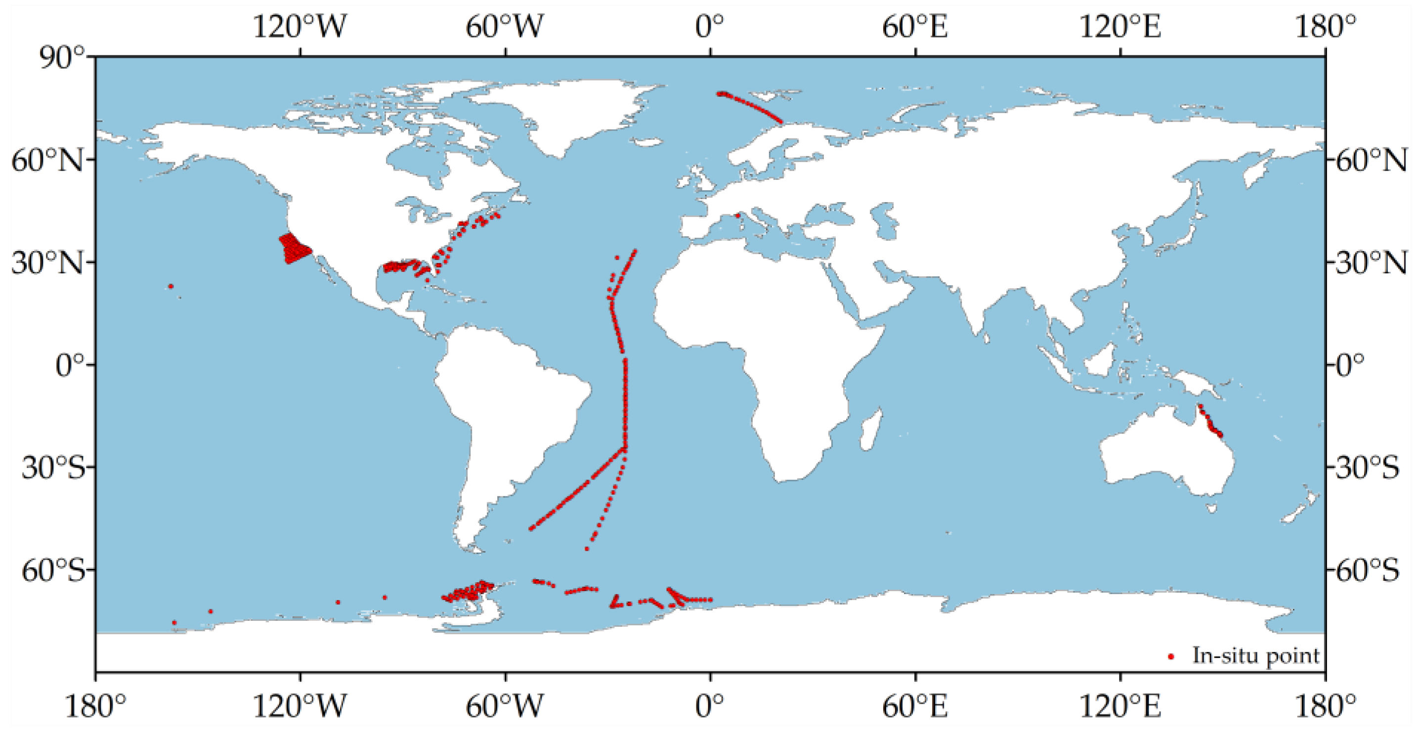
2.2.2. In-Situ Data

There are numerous in-situ measurements of global chlorophyll-a concentrations. Here, we selected the global bio-optical in-situ data compilation used by OC-CCI for ocean color satellite applications. This dataset has been updated to its third version, with the latest in-situ data updated to January 2021. However, there are only 17 in-situ measurements from 2020 to 2021, so we chose to validate using measured data from 2017 to 2019. A total of 1526 in-situ measurements from January, April, July, and October of 2017, 2018, and 2019 were selected. After excluding points that were not suitable for inversion (i.e., those without remote sensing reflectance data), we had 1239 remaining points. Figure 1 shows the distribution of the selected in-situ measurement points after exclusion.

2.2.3. Data Preprocessing

Due to various reasons, such as data anomalies, algorithm errors, and lighting conditions, the remote sensing reflectance may produce abnormal values less than zero. Therefore, it is necessary to eliminate these abnormal values in the remote sensing reflectance before performing the inversion, providing a solid foundation for the subsequent logarithmic transformation. Since the number of abnormal values is small, they have almost no impact on the inversion of the global ocean as a whole. Reflectance data typically exhibits a wide dynamic range, with significant differences in reflectance across different wavebands and features. Applying a logarithmic transformation to the reflectance data can reduce this variability, enabling more accurate comparisons between different datasets, thereby improving the convergence of the inversion algorithm and enhancing the accuracy of the inversion results. Therefore, a log10(lg) transformation is applied to the global ocean remote sensing reflectance, serving as an independent variable for subsequent inversion and facilitating model training. In terms of software usage, SPSS 27 was utilized for data analysis, Origin 2022 was used for data visualization and plotting, and ArcGIS 10.8 was employed for map processing and spatial analysis.

2.3. Methods

2.3.1. Temperature Zoning Idea

The core of the chlorophyll-a inversion work in this article focuses on temperature zoning. The correlation between temperature and chlorophyll-a concentration has been established, and there exists a mapping relationship between band ratios and chlorophyll-a concentration. Therefore, this article hypothesizes that different temperature conditions can influence the mapping relationship between band ratios and chlorophyll-a, proposing the concept of temperature zoning during the inversion process. If this hypothesis holds true, then using a mapping relationship adjusted based on temperature zoning for chlorophyll-a inversion would result in improved inversion accuracy. To ensure the averageness of the zoning, temperature zoning was performed for the global ocean based on the monthly average OISST data for October 2018, according to the temperature frequency distribution of the inversion samples. After preprocessing the available data, the selected variables were used to construct the inversion model in conjunction with the inversion set based on the temperature zoning. The developed OC3V_(SST) model was then applied for validation to the data from January, April, July, and October of 2017, 2018, and 2019, covering a total of 12 months, as well as the entire month of October 2018, spanning 31 days. Figure 2 depicts the chlorophyll-a inversion workflow based on the concept of temperature zoning.

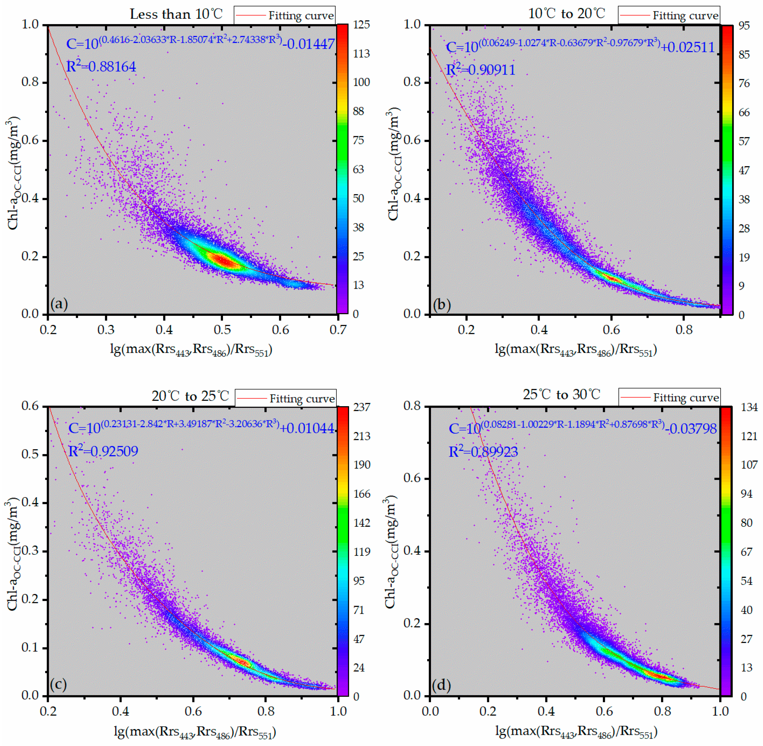
2.3.2. OC3V Inversion Algorithm Based on Temperature Zoning

In terms of inversion algorithms, this article introduces two classic ocean chlorophyll-a algorithms (OC2 and OC3). Since both algorithms are well-established, the selection of the algorithm in this article was made by choosing the better-performing one among the two. The OC2 and OC3 algorithms are based on a MCP, and Equation (1) is as follows:

$$C={10}^{\left(a0+a1\ast R+a2\ast R^2+a3\ast R^3\right)}+a4$$

(1)

In Equation (1), $C$ represents the chlorophyll-a concentration, $R$ stands for the band ratio, and $a0$, $a1$, $a2$, $a3$, and $a4$ are coefficients.

In ocean chlorophyll-a algorithms, the transition from a single-term polynomial with two coefficients to a cubic polynomial with five coefficients represents an improvement in accuracy. This algorithm has proven to be the most precise among those designed for the VIIRS sensor for measuring ocean chlorophyll-a. Originally, this algorithm was developed for the SeaWiFS sensor. However, with the advent of the VIIRS sensor, the algorithm was adapted and extended to it, resulting in the OC2V and OC3V algorithms.

Table 1. Band ratios and coefficients for OC2V and OC3V.

Algorithm	Band Ratio(R)	Coefficient
		a0	a1	a2	a3	a4
OC2V	lg(Rrs486/Rrs551)	0.3410	−3.0010	2.8110	−2.0410	−0.0400
OC3V	lg(max(Rrs443,Rrs486)/Rrs551)	0.3483	−2.9959	2.9873	−1.4813	−0.0597

shows the band ratios and coefficients for OC2V and OC3V.

By using two inversion algorithms, the global monthly average oceanic chlorophyll-a concentration for October 2018 was retrieved and compared for accuracy, allowing for the selection of independent variable parameters for the inversion process. Within each predefined temperature range, an improved cubic polynomial inversion model, OC3V_(SST), was constructed based on band ratios and chlorophyll-a concentrations. To build this model, the inversion set was created using the independent variables determined from the monthly average remote sensing reflectance data of VIIRS. The OC-CCI monthly average chlorophyll-a concentration data served as the chlorophyll-a concentration for the inversion points. The MCP algorithm was employed to establish the mapping relationship between the independent variables and chlorophyll-a concentrations, thus determining the values of the five parameters. This ultimately led to the development of the OC3V_(SST) inversion algorithm for each temperature range.

2.3.3. Precision Evaluation Index

The accuracy of the chlorophyll-a inversion model was evaluated using the coefficient of determination (R²), root mean square error (RMSE), mean absolute error (MAE), and mean relative error (MRE).

In Equation (2), R² is the most commonly used index to judge the degree of fitting of regression models. In Equation (3), RMSE is used to measure the deviation between the predicted value and the measured value. In Equation (4), MAE is the average value of the absolute error. In Equation (5), MRE is the average of the relative errors. The expression of Equations (2)–(5) is as follows:

$$R^2=\frac{{\displaystyle {\sum }_{i=1}^n{\left(y_i-{\widehat{y}}_i\right)}^2}}{{\displaystyle {\sum }_{i=1}^n{\left(y_i-{\overline{y}}_i\right)}^2}}$$

(2)

$$RMSE=\sqrt{\frac{1}{n}{\displaystyle \sum _{i=1}^n{\left(y_i-{\widehat{y}}_i\right)}^2}}$$

(3)

$$MAE=\frac{1}{n}{\displaystyle \sum _{i=1}^n\left|y_i-{\widehat{y}}_i\right|}$$

(4)

$$MRE=\frac{1}{n}{\displaystyle \sum _{i=1}^n\left|\frac{y_i-{\widehat{y}}_i}{y_i}\right|}\times 100\%$$

(5)

In Equations (2)–(5), n represents the number of sample points; $y_i$ represents the true chlorophyll-a concentration value of the i-th sample point; ${\widehat{y}}_i$ represents the predicted concentration value of the i-th sample point; ${\overline{y}}_i$ represents the mean value of the true chlorophyll-a concentration.

3. Results

3.1. Temperature Zoning Result

The global range was divided into regions measuring 1° × 1° (totaling 64,800 regions) and 2° × 2° (totaling 16,200 regions), and these regions were then trimmed to exclude areas outside the global oceanic extent. To ensure the stability and accuracy of the inversion algorithm while also considering the need for a sufficient number of inversion samples and the limitations of the processing software, a 4:1 ratio between the number of inversion samples and validation samples was adopted. Specifically, two points were randomly selected from each 1° × 1° region as sample points, and two points were randomly selected from each 2° × 2° region as validation points.

By incorporating temperature factors into the inversion process, we aim to enhance the efficiency and accuracy of the inversion. Therefore, the global ocean temperature range (−1.8 °C to 32.4 °C) is divided into different gradient ranges. Since our inversion samples are selected with reasonable and comprehensive spatial coverage, the temperature frequency of the inversion samples can be used as the basis for temperature zoning. By adopting a temperature gradient of 10 °C, the global ocean is divided into temperature zones. Based on the temperature frequency, the frequency of temperatures ranging from 20 °C to 30 °C is approximately twice that of the other temperature intervals, with 25 °C as the midpoint of the frequency. After taking into account the average distribution of the zones, the temperature range was evenly divided into four temperature ranges: less than 10 °C, 10 °C to 20 °C, 20 °C to 25 °C, and 25 °C to 30 °C (the actual maximum was 32.4 °C, rounded to 30 °C for convenience). The temperature frequency and zoning results are shown in Figure 3.

3.2. Determination of Inversion Independent Variables

The selection of independent variables is essential for inversion. In this paper, two classical ocean chlorophyll-a inversion models (OC2 and OC3) are introduced to perform inversion over the global ocean. The independent variable for the OC2 model is lg(Rrs₄₈₆/Rrs₅₅₁), while the independent variable for the OC3 model is lg(max(Rrs₄₄₃,Rrs₄₈₆)/Rrs₅₅₁). By comparing the inversion results of the two models, the optimal model was selected, thereby determining the inversion independent variable. The results are shown in Figure 4.

Based on the inversion results, it is evident that the OC3 model exhibits lower RMSE, MAE, and MRE compared to the OC2 model. Therefore, for subsequent inversion work, the independent variable selected was the one used in the OC3 model, which is lg(max(Rrs₄₄₃,Rrs₄₈₆)/Rrs₅₅₁).

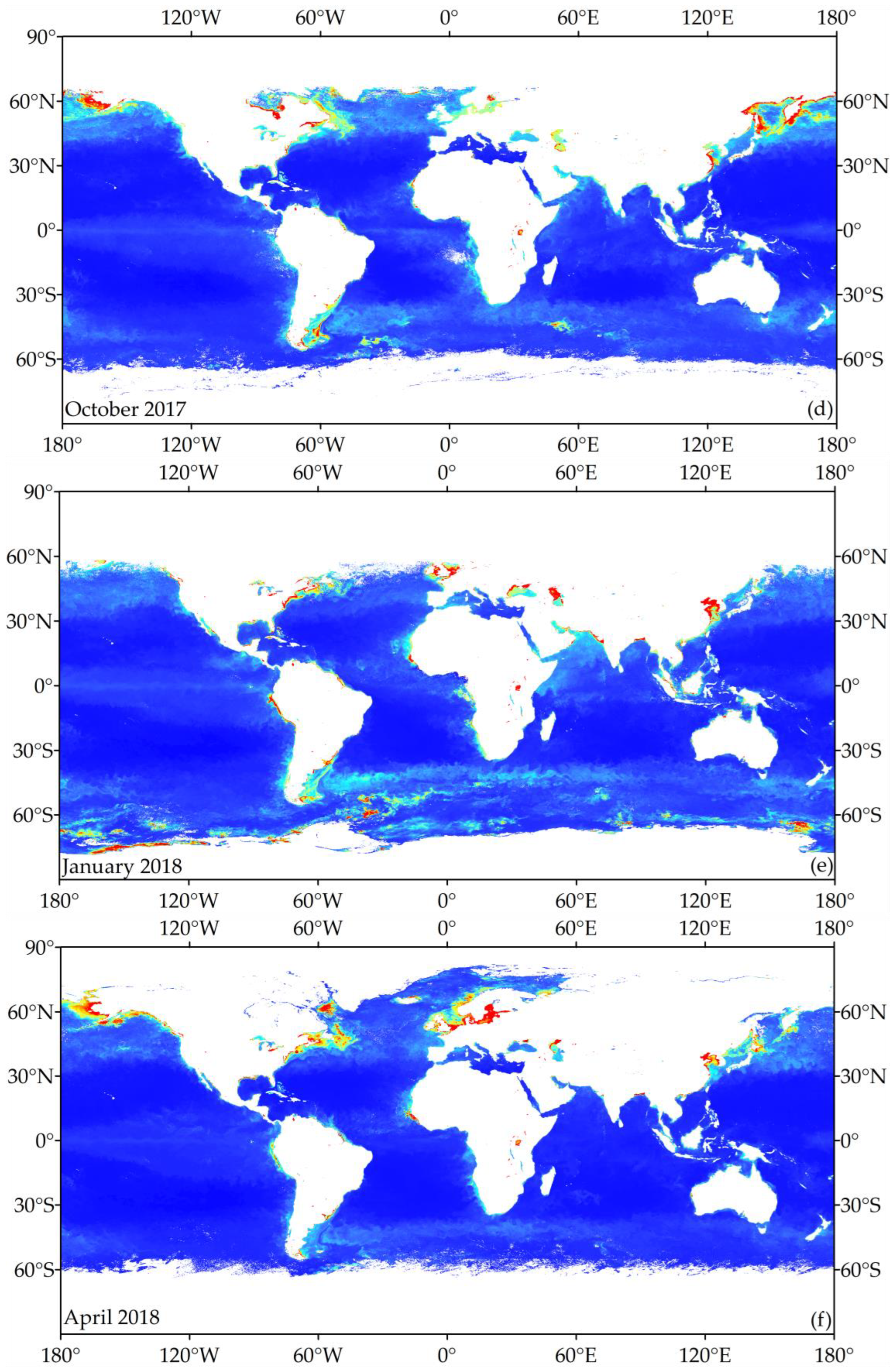
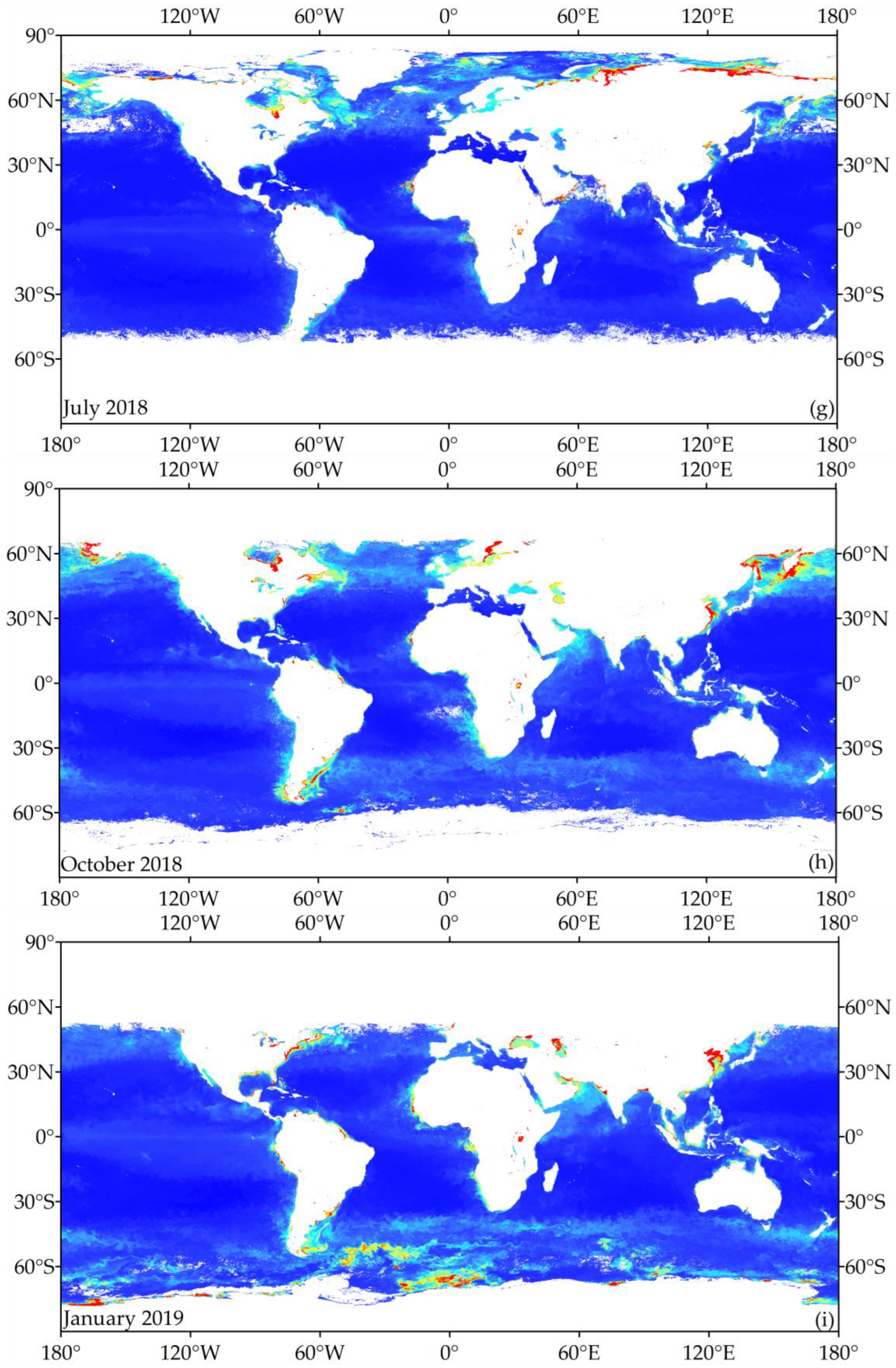
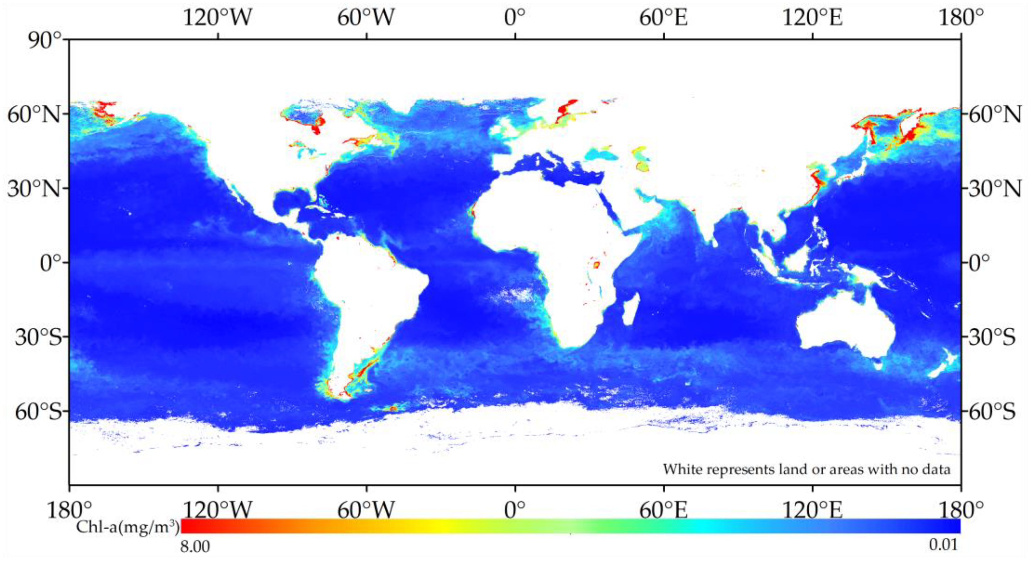
3.3. Global Chlorophyll-a Concentration

Using the three-band ratio of lg(max(Rrs₄₄₃,Rrs₄₈₆)/Rrs₅₅₁) as the input parameter, an OC3V_(SST) inversion model was constructed, with the OC-CCI chlorophyll-a concentration of the inversion sample points serving as the target chlorophyll-a concentration. Both VIIRS and OC-CCI daily products contain significant gaps, and using them for modeling would severely limit the global applicability of the model. After taking into account the need for comprehensive global inversion, monthly average data were selected for model development. Given the abundance of measured data available for October 2018, which allows for a more precise validation of the model’s accuracy, remote sensing data from October 2018 was chosen for modeling. Figure 5 depicts the fitting plot of the OC3V_(SST) inversion algorithm,

Table 2. Content of the OC3V_(SST) algorithm.

Inversion Range	OC3V(SST) *
Less than 10 °C	$C={10}^{\left(0.4616-2.03633\ast R-1.85074\ast R^2+2.74338\ast R^3\right)}-0.01447$
10–20 °C	$C={10}^{\left(0.06249-1.0274\ast R-0.63679\ast R^2-0.97679\ast R^3\right)}+0.02511$
20–25 °C	$C={10}^{\left(0.23131-2.842\ast R+3.49187\ast R^2-3.20636\ast R^3\right)}+0.01044$
25–30 °C	$C={10}^{\left(0.08281-1.00229\ast R-1.1894\ast R^2+0.87698\ast R^3\right)}-0.03798$

* C is the concentration of chlorophyll-a, and R is lg(max(Rrs₄₄₃,Rrs₄₈₆)/Rrs₅₅₁).

summarizes the details of the constructed OC3V_(SST) inversion model, and Figure 6 displays the inversion results obtained from the OC3V_(SST) model(The following exhibits only the inversion result map for October 2018, which was displayed, while the inversion result maps for all the months were presented in Figure A1 of the Appendix A). The inversion results are in the form of raster data, comprising a total of 18,680,581 raster cells. Due to the rarity of high-value raster cells, for the purpose of clarity in the presentation, only values ranging from 0.01 mg/m³ to 8.00 mg/m³ are displayed.

When performing fitting, the Levenberg–Marquardt optimization algorithm was adopted, which exhibits excellent adaptability and robustness in handling nonlinear fitting problems. It is capable of handling more complex data and models, finding the optimal solution through iterative optimization. The content of the fitting parameters and the corresponding errors are summarized in

Table 3. Parameter fitting error summary.

Temperature Interval	a0		a1		a2		a3		a4		Statistics
	Value	Standard Error	Value	Standard Error	Value	Standard Error	Value	Standard Error	Value	Standard Error	Reduced Chi-Sqr	R2
Less than 10 °C	0.4616	0.00534	−2.03633	0.02842	−1.85074	0.15734	2.74338	0.1961	−0.01447	0.03645	0.00352	0.88164
10–20 °C	0.06249	0.01131	−1.0274	0.11553	−0.63679	0.35079	−0.97679	0.37967	0.02511	0.00374	0.00251	0.90911
20–25 °C	0.23131	0.00576	−2.842	0.06537	3.49187	0.18816	−3.20636	0.17662	0.01044	0.00163	0.00055	0.92509
25–30 °C	0.08281	0.01873	−1.00229	0.04679	−1.1894	0.1006	0.87698	0.2711	−0.03798	0.04751	0.00122	0.89923

.

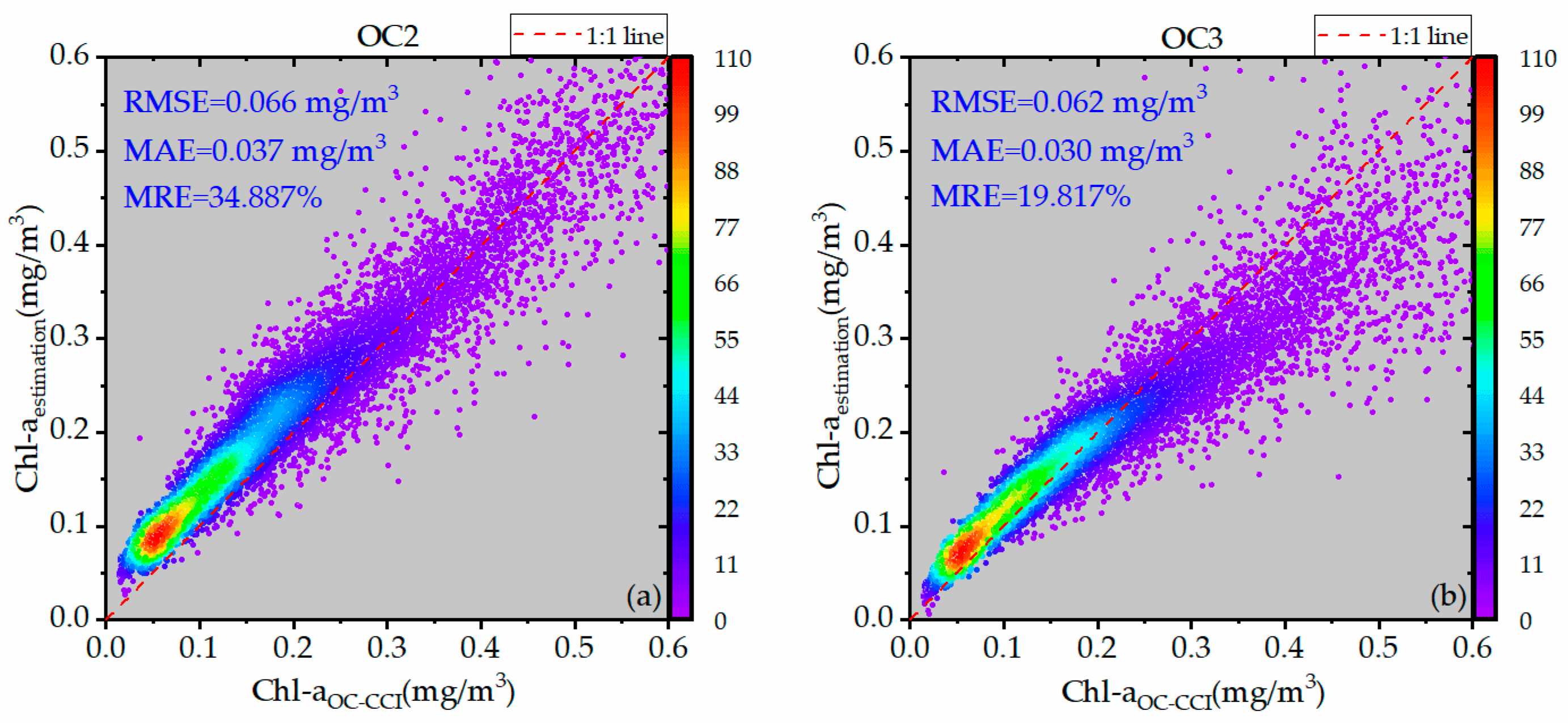
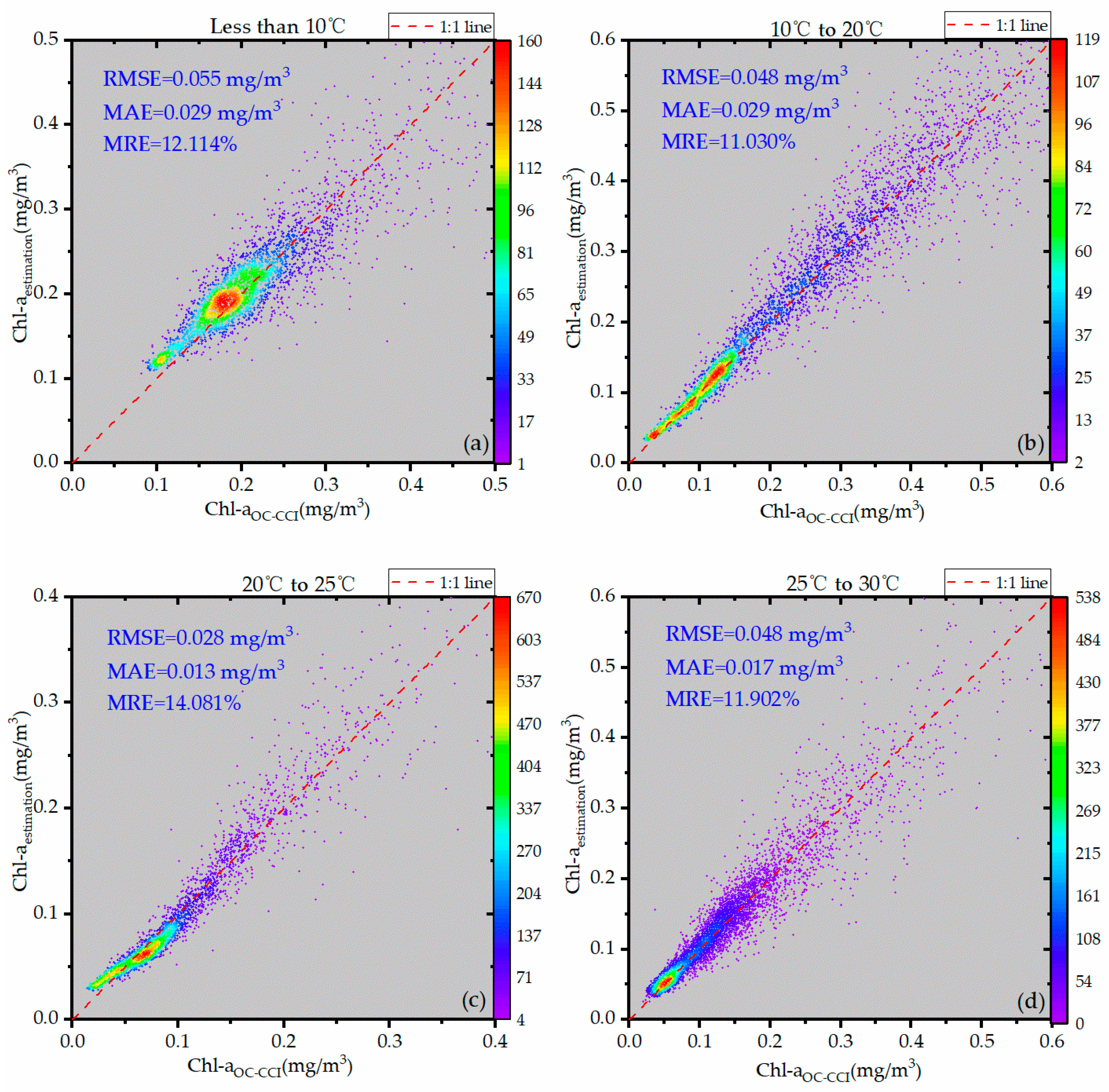
3.4. Accuracy Verification

Based on the constructed OC3V_(SST) inversion model, the inversion process was applied to a set of validation points, and the accuracy was verified. Since there were no measured data available for the validation points, the error between the inverted concentrations and OC-CCI was used for validation. Figure 7 illustrates the verification of inversion accuracy across four temperature regions.

Based on the inversion results, the accuracy validation statistics are as follows: for the region with a temperature range below 10 °C, the inversion yields a RMSE of 0.055 mg/m³, a MAE of 0.029 mg/m³, and a MRE of 12.114%; for the region with a temperature range from 10 °C to 20 °C, the inversion RMSE is 0.048 mg/m³, the MAE is 0.029 mg/m³, and the MRE is 11.03%; for the region with a temperature range from 20 °C to 25 °C, the inversion RMSE is 0.028 mg/m³, the MAE is 0.013 mg/m³, and the MRE is 14.081%; finally, for the region with a temperature range from 25 °C to 30 °C, the inversion RMSE is 0.048 mg/m³, the MAE is 0.017 mg/m³, and the MRE is 11.902%. These validation statistics are summarized in

Table 4. Accuracy validation comparison between the OC3V_(SST) inversion algorithm and the classic OC3V chlorophyll-a inversion algorithm.

Inversion Range	Model Formula	RMSE (mg/m3)	MAE (mg/m3)	MRE
All areas	OC3V	0.062	0.030	19.8%
Less than 10 °C	OC3V(SST)	0.055	0.029	12.1%
10–20 °C	OC3V(SST)	0.048	0.029	11.0%
20–25 °C	OC3V(SST)	0.028	0.013	14.1%
25–30 °C	OC3V(SST)	0.048	0.017	11.9%

.

Due to the coarseness of monthly scale data inversion, the model was applied to the daily remote sensing reflectance data of October 2018, excluding the measured points with blank remote sensing reflectance. Accuracy validation of daily scale inversion was performed based on the measured data.

Table 5. Accuracy validation table of OC3V_(SST) inversion results versus OC3V inversion results for 31 days of measured points in October 2018.

Model Formula	RMSE (mg/m3)	MAE (mg/m3)	MRE
OC3V	7.479	1.175	70.1%
OC3V(SST)	0.678	0.272	37.9%

presents the accuracy validation table of the OC3V_(SST) inversion results of the measured points for a total of 31 days in October 2018, compared to the classic OC3V chlorophyll-a inversion results.

Considering the potential phenological biases during the autumn in the Northern Hemisphere and spring in the Southern Hemisphere, the inversion model was applied to the months of January, April, July, and October in 2017, 2018, and 2019, and the accuracy of these months was validated.

Table 6. Deviation table of OC3V and OC3V_(SST) inversion results relative to OC-CCI for validation points.

Time	Model Formula	RMSE (mg/m3)	MAE (mg/m3)	MRE
January 2017	OC3V	0.286	0.035	21.1%
	OC3V(SST) (Less than 10 °C)	0.107	0.058	18.4%
	OC3V(SST) (10–20 °C)	0.063	0.035	12.9%
	OC3V(SST) (20–25 °C)	0.022	0.011	11.1%
	OC3V(SST) (25–30 °C)	0.097	0.021	13.9%
April 2017	OC3V	0.509	0.037	19.9%
	OC3V(SST) (Less than 10 °C)	0.115	0.052	17.2%
	OC3V(SST) (10–20 °C)	0.101	0.050	15.8%
	OC3V(SST) (20–25 °C)	1.060	0.036	17.5%
	OC3V(SST) (25–30 °C)	0.050	0.017	12.4%
July 2017	OC3V	0.095	0.029	19.4%
	OC3V(SST) (Less than 10 °C)	0.147	0.079	22.4%
	OC3V(SST) (10–20 °C)	0.067	0.034	12.8%
	OC3V(SST) (20–25 °C)	0.110	0.020	13.3%
	OC3V(SST) (25–30 °C)	0.046	0.019	14.9%
October 2017	OC3V	0.107	0.031	19.9%
	OC3V(SST) (Less than 10 °C)	0.089	0.039	12.7%
	OC3V(SST) (10–20 °C)	0.063	0.036	13.0%
	OC3V(SST) (20–25 °C)	0.061	0.014	10.4%
	OC3V(SST) (25–30 °C)	0.065	0.018	12.6%
January 2018	OC3V	0.083	0.033	21.7%
	OC3V(SST) (Less than 10 °C)	0.114	0.055	16.5%
	OC3V(SST) (10–20 °C)	0.060	0.035	12.5%
	OC3V(SST) (20–25 °C)	0.040	0.014	11.5%
	OC3V(SST) (25–30 °C)	0.049	0.019	14.2%
April 2018	OC3V	0.095	0.032	20.0%
	OC3V(SST) (Less than 10 °C)	0.110	0.052	18.2%
	OC3V(SST) (10–20 °C)	0.075	0.044	15.8%
	OC3V(SST) (20–25 °C)	0.032	0.013	15.6%
	OC3V(SST) (25–30 °C)	0.042	0.016	12.0%
July 2018	OC3V	0.077	0.030	20.0%
	OC3V(SST) (Less than 10 °C)	0.123	0.074	22.7%
	OC3V(SST) (10–20 °C)	0.067	0.033	12.9%
	OC3V(SST) (20–25 °C)	0.097	0.019	12.2%
	OC3V(SST) (25–30 °C)	0.052	0.020	15.9%
October 2018	OC3V	0.062	0.030	19.8%
	OC3V(SST) (Less than 10 °C)	0.055	0.029	12.1%
	OC3V(SST) (10–20 °C)	0.048	0.029	11.0%
	OC3V(SST) (20–25 °C)	0.028	0.013	14.1%
	OC3V(SST) (25–30 °C)	0.048	0.017	11.9%
January 2019	OC3V	0.226	0.038	20.7%
	OC3V(SST) (Less than 10 °C)	0.105	0.058	15.4%
	OC3V(SST) (10–20 °C)	0.063	0.036	12.4%
	OC3V(SST) (20–25 °C)	0.037	0.012	11.3%
	OC3V(SST) (25–30 °C)	0.342	0.027	13.8%
April 2019	OC3V	0.124	0.033	18.7%
	OC3V(SST) (Less than 10 °C)	0.104	0.049	17.1%
	OC3V(SST) (10–20 °C)	0.076	0.045	15.7%
	OC3V(SST) (20–25 °C)	0.078	0.015	14.0%
	OC3V(SST) (25–30 °C)	0.328	0.025	12.0%
July 2019	OC3V	0.075	0.029	17.7%
	OC3V(SST) (Less than 10 °C)	0.112	0.070	26.3%
	OC3V(SST) (10–20 °C)	0.079	0.039	13.9%
	OC3V(SST) (20–25 °C)	0.168	0.025	13.2%
	OC3V(SST) (25–30 °C)	0.048	0.017	1.7%
October 2019	OC3V	0.090	0.032	19.2%
	OC3V(SST) (Less than 10 °C)	0.121	0.042	12.5%
	OC3V(SST) (10–20 °C)	0.062	0.033	11.2%
	OC3V(SST) (20–25 °C)	0.035	0.013	10.3%
	OC3V(SST) (25–30 °C)	0.037	0.015	1.5%

presents the deviation results of the OC3V inversion results and OC3V_(SST) inversion results relative to OC-CCI for the validation points.

Table 7. Comparison of accuracy between OC-CCI, OC3V inversion results, and OC3V_(SST) inversion results for measured points.

Time	Model Formula	RMSE (mg/m3)	MAE (mg/m3)	MRE
January 2017	OC-CCI	1.325	0.645	108.9%
	OC3V	2.584	0.867	146.4%
	OC3V(SST)	1.242	0.524	82.6%
April 2017	OC-CCI	2.150	1.010	98.2%
	OC3V	2.366	1.254	166.2%
	OC3V(SST)	2.049	0.791	72.9%
July 2017	OC-CCI	1.363	0.666	105.1%
	OC3V	4.385	1.390	128.8%
	OC3V(SST)	0.717	0.467	91.1%
October 2017	OC-CCI	2.057	0.913	74.0%
	OC3V	4.882	1.953	126.2%
	OC3V(SST)	2.496	0.936	56.7%
January 2018	OC-CCI	2.431	1.251	138.6%
	OC3V	3.114	1.890	221.5%
	OC3V(SST)	2.510	1.126	92.1%
April 2018	OC-CCI	2.286	0.921	92.8%
	OC3V	2.285	1.107	153.7%
	OC3V(SST)	2.259	0.882	78.9%
July 2018	OC-CCI	0.483	0.218	32.9%
	OC3V	3.146	1.138	64.3%
	OC3V(SST)	1.518	0.600	51.8%
October 2018	OC-CCI	0.389	0.181	45.3%
	OC3V	0.580	0.236	59.6%
	OC3V(SST)	0.326	0.167	43.6%
January 2019	OC-CCI	2.059	1.228	72.4%
	OC3V	2.433	1.565	96.5%
	OC3V(SST)	2.177	1.249	57.9%
April 2019	OC-CCI	1.767	0.613	59.1%
	OC3V	1.985	0.724	109.1%
	OC3V(SST)	1.849	0.627	67.5%
July 2019	OC-CCI	2.401	0.902	76.3%
	OC3V	2.391	0.959	106.7%
	OC3V(SST)	2.696	1.039	88.5%
October 2019	OC-CCI	0.016	0.008	7.2%
	OC3V	0.008	0.008	7.8%
	OC3V(SST)	0.014	0.012	10.4%

compares the accuracy of OC-CCI, OC3V inversion results, and OC3V_(SST) inversion results for the measured points.

Due to the proximity of most measured points to land, global ocean chlorophyll-a inversion algorithms tend to underestimate chlorophyll-a concentration in coastal areas, leading to larger errors at measured points compared to sample points. It should be noted that the validation for October 2019 is of limited significance as there was only one measured point available. From the aforementioned results, it is apparent that all four constructed inversion models exhibit improved accuracy compared to the classical OC3V model. This suggests that incorporating temperature range segmentation into the inversion of chlorophyll-a concentration significantly enhances inversion accuracy. This underscores the critical influence of temperature on the distribution of chlorophyll-a concentration and affirms the relevance of the temperature zoning approach in chlorophyll-a inversion efforts.

4. Discussion

4.1. Spatial Distribution Analysis

In exploring the spatial distribution of a certain element, three common spatial analysis methods are typically introduced: spatial autocorrelation analysis, clustering and outlier analysis, and hotspot analysis. These three methods are frequently utilized in spatial analysis. Moreover, there are studies that apply these methods to investigate the spatial distribution of chlorophyll-a concentration [57]. Often, these three methods are used simultaneously [58,59,60]. Among them, spatial autocorrelation analysis is used to determine spatial correlation, clustering and outlier analysis is applied to classify similar chlorophyll-a concentration areas or detect regions with chlorophyll-a concentrations that significantly deviate from the average, and hotspot analysis is employed to identify statistically significant hotspots and coldspots, which represent the aggregation or dispersion of chlorophyll-a concentration.

Based on the defined temperature ranges, we delve into the spatial distribution characteristics of chlorophyll-a concentration across various temperature regimes. We utilized three spatial analysis techniques to investigate the spatial distribution of chlorophyll-a in October 2018: spatial autocorrelation analysis, clustering and outlier detection, and hotspot analysis.

4.1.1. Spatial Autocorrelation Analysis

To determine the existence of spatial correlation in chlorophyll-a concentration across different temperature ranges, Moran’s I index is introduced here. Moran’s I is a crucial indicator in geospatial data analysis, used to measure the spatial autocorrelation present in geospatial data. The calculation of Moran’s I index involves computing the spatial weights between data points on a map and then multiplying this weight matrix with the vector of data values to obtain the Moran’s I index results. The Moran’s I index typically yields a value between −1 and +1. A result close to +1 indicates a strong positive spatial autocorrelation in the data, whereas a result close to −1 suggests a strong negative spatial autocorrelation. If the index result is close to 0, it implies a random spatial distribution of the data. By applying Moran’s I index to our analysis, we can gain insights into the spatial patterns and dependencies of chlorophyll-a concentration across the defined temperature ranges.

Moran’s I index can be expressed as follows:

$$I=\frac{n}{S_0}\frac{{\displaystyle \sum _{i=1}^n{\displaystyle \sum _{j=1}^n{\omega }_{i,j}{z}_i{z}_j}}}{{\displaystyle \sum _{i=1}^n{z}_i^2}}$$

(6)

where $z_i$ is the deviation of the attribute of factor $i$ from its mean (x_i − x), $w_{i,j}$ is the spatial weight between factor $i$ and $j$, $n$ is equal to the total number of factors, and $S_0$ is the aggregate of all spatial weights:

$$S_0={\displaystyle \sum _{i=1}^n{\displaystyle \sum _{j=1}^n{\omega }_{i,j}}}$$

(7)

Z-scores are calculated in the following form:

$$z=\frac{I-E\left[I\right]}{\sqrt{V\left[I\right]}}$$

(8)

where:

$$E\left[I\right]=\frac{-1}{n-1}$$

(9)

$$V\left[I\right]=E\left[I^2\right]-E{\left[I\right]}^2$$

(10)

The p-value (probability value) represents a probability. For pattern analysis tools, the p-value indicates the probability that the observed spatial pattern is created by a certain random process. When the p-value is very small, it means that the observed spatial pattern is unlikely to arise from a random process (a low-probability event). Therefore, the null hypothesis can be rejected. The z-score represents multiples of the standard deviation, and a higher z-value indicates a higher degree of clustering. Both the z-score and the p-value can be used to determine whether to reject the null hypothesis.

Table 8. Index table of spatial autocorrelation analysis.

Temperature Range	The Moran I Index	z-Score	p-Value
Less than 10 °C	0.356	955.8	0.000
10 °C to 20 °C	0.591	370.1	0.000
20 °C to 25 °C	0.273	536.2	0.000
25 °C to 30 °C	0.497	255.9	0.000

shows the index results of spatial autocorrelation analysis.

Based on the above results, the p-values for all four ranges are less than 0.01, indicating that the possibility of randomly generating such a clustering pattern is less than 1%. In other words, the spatial distribution of chlorophyll-a is correlated and exhibits a clustered distribution.

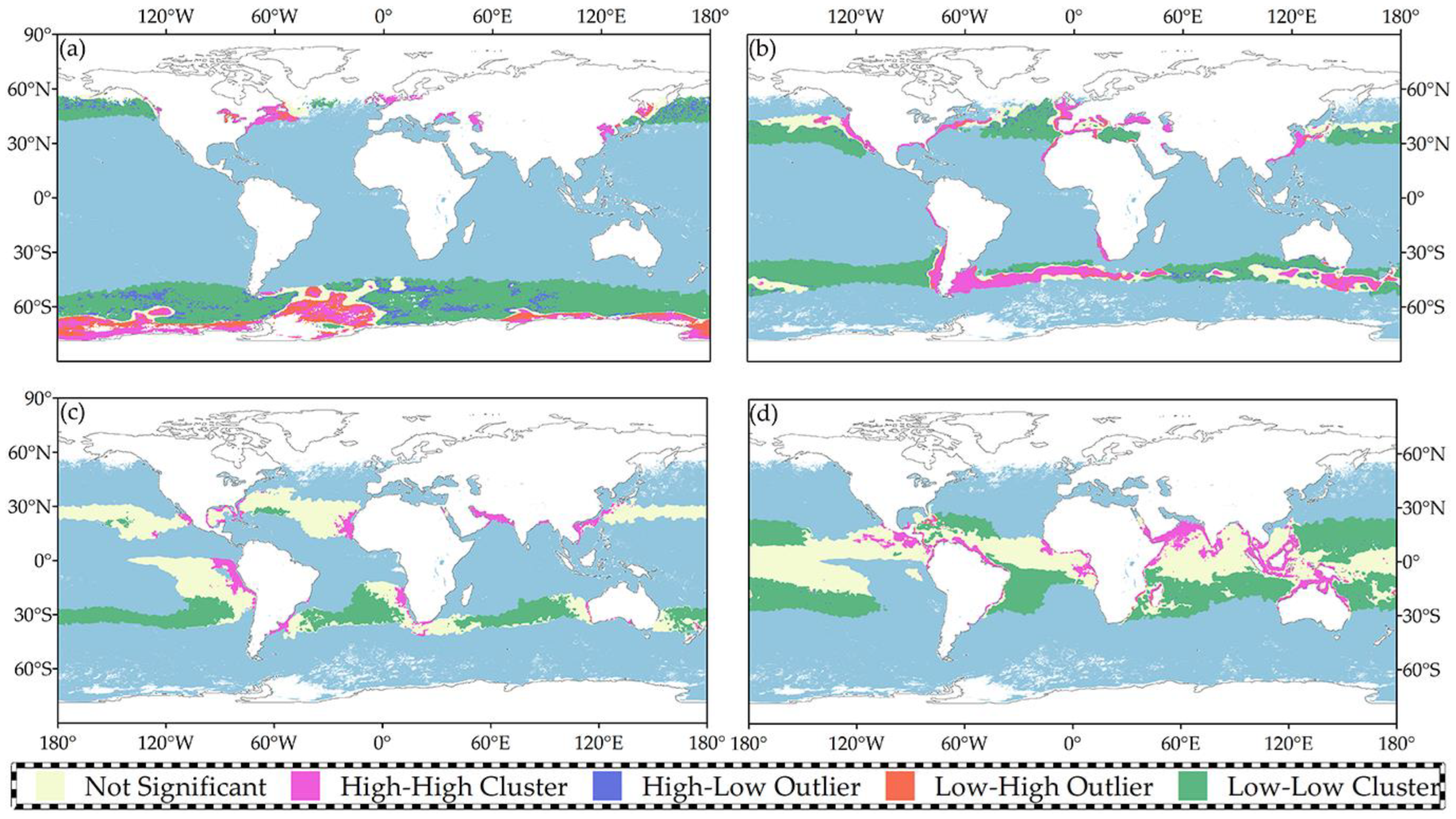
4.1.2. Clustering and Outlier Analysis

The Local Moran’s I statistic for spatial association is defined as follows:

$$I_i=\frac{x_i-\overline{X}}{S_i^2}{\displaystyle \sum _{j=1,j\ne i}^n{w}_{i,j}\left(x_j-\overline{X}\right)}$$

(11)

where $x_i$ is the attribute of feature $i$, $\overline{X}$ is the mean of the corresponding attribute, $w_{i,j}$ is the spatial weight between feature $i$ and $j$, and:

$$S_i^2=\frac{{\displaystyle \sum _{j=1,j\ne i}^n{\left(x_j-\overline{X}\right)}^2}}{n-1}$$

(12)

n equals the total number of features.

The calculation of the $z_{I_i}$ score for the statistic is as follows:

$$z_{I_i}=\frac{I_i-E\left[I_i\right]}{\sqrt{V\left[I_i\right]}}$$

(13)

where;

$$E\left[I_i\right]=-\frac{{\displaystyle \sum _{j=1,j\ne i}^n{w}_{ij}}}{n-1}$$

(14)

$$V\left[I_i\right]=E\left[{I_i}^2\right]-E{\left[I_i\right]}^2$$

(15)

Based on the global Moran’s I index, it can be inferred that the distribution of chlorophyll-a concentrations within the four temperature ranges exhibits a certain regularity. Therefore, a clustering and outlier analysis was conducted on the chlorophyll-a concentrations within these four temperature ranges. The analysis evaluated four indicators: high-value clustering, low-value clustering, low values surrounded by high values, and high values surrounded by low values. High-value clustering and low-value clustering are collectively referred to as clustering, while low values surrounded by high values and high values surrounded by low values are collectively termed outliers. The results of the clustering and outlier analysis are presented in Figure 8.

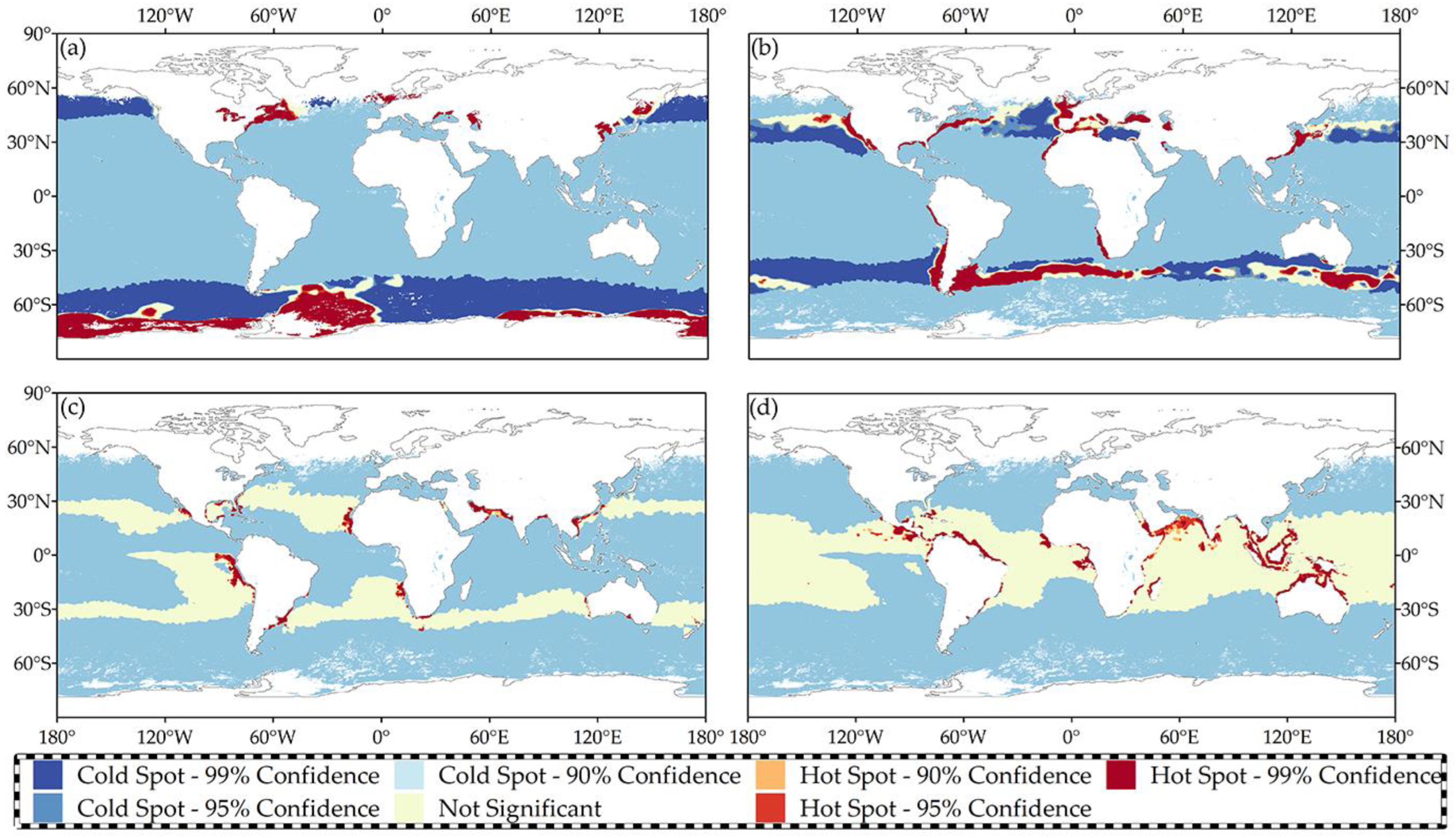
4.1.3. Hotspot Analysis

The Getis–Ord local statistic can be expressed as follows:

$$G_i^{*}=\frac{{\displaystyle \sum _{j=1}^n{w}_{i,j}{x}_j-\overline{X}{\displaystyle \sum _{j=1}^n{w}_{i,j}}}}{S\sqrt{\frac{\left[n{\displaystyle \sum _{j=1}^n{w}_{i,j}^2-{\left({\displaystyle \sum _{j=1}^n{w}_{i,j}}\right)}^2}\right]}{n-1}}}$$

(16)

where $x_j$ is the attribute value of feature $j$, $w_{i,j}$ is the spatial weight between feature $i$ and $j$, n is the total number of features, and:

$$\overline{X}=\frac{{\displaystyle \sum _{j=1}^n{x}_j}}{n}$$

(17)

$$S=\sqrt{\frac{{\displaystyle \sum _{j=1}^n{x}_j^2}}{n}-{\left(\overline{X}\right)}^2}$$

(18)

The $G_i^{*}$ statistic returned for each feature in the dataset is a z-score. For statistically significant positive z-scores, the higher the z-score, the more tightly clustered the high values (hot spots) are. For statistically significant negative z-scores, the lower the z-score, the more tightly clustered the low values (cold spots) are. The cold and hot spot analysis of chlorophyll-a concentrations across four temperature ranges is presented in Figure 9.

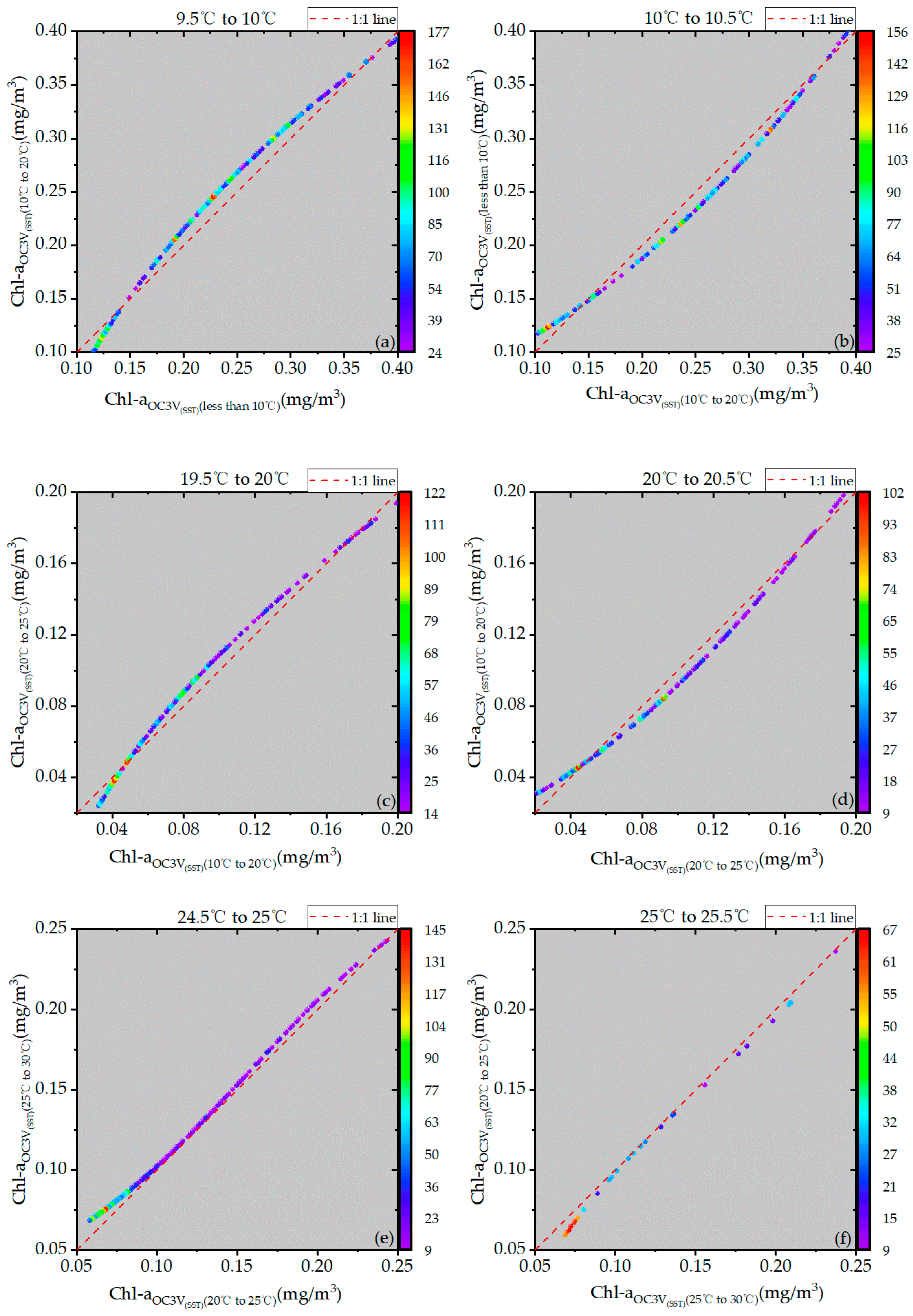
4.2. Continuity Analysis

Due to the construction of four different inversion models for the global ocean in this paper, there are inevitably issues of spatial and temporal discontinuity in the inversion results, which are ultimately caused by temperature zoning. Therefore, we investigated the continuity of the models at the intersections of the four temperature regions. In the adjacent sections between every two temperature zones, six regions with a temperature width of 0.5 °C were selected: 9.5 °C–10 °C, 10 °C–10.5 °C, 19.5 °C–20 °C, 20 °C–20.5 °C, 24.5 °C–25 °C, and 25 °C–25.5 °C. Continuity tests were conducted in these regions by comparing the inversion values obtained from the inversion models of neighboring temperature regions using the remote sensing reflectance of the validation points in each region. Figure 10 displays the comparison results, and

Table 9. Error table for the six regions.

Temperature Range	RMSE (mg/m3)	MAE (mg/m3)	MRE
9.5 °C–10 °C	0.013	0.013	5.9%
10 °C–10.5 °C	0.013	0.011	5.0%
19.5 °C–20 °C	0.006	0.005	7.2%
20 °C–20.5 °C	0.006	0.005	7.5%
24.5 °C–25 °C	0.005	0.005	5.9%
25 °C–25.5 °C	0.005	0.005	5.0%

provides the corresponding accuracy metrics. The accuracy validation of the normal inversion results for the validation points in these regions against the OC-CCI product is presented in

Table 10. Verification table for normal inversion results.

Temperature Range	RMSE (mg/m3)	MAE (mg/m3)	MRE
9.5 °C–10 °C	0.064	0.041	12.9%
10 °C–10.5 °C	0.068	0.040	10.9%
19.5 °C–20 °C	0.046	0.019	13.1%
20 °C–20.5 °C	0.027	0.013	10.2%
24.5 °C–25 °C	0.022	0.012	10.2%
25 °C–25.5 °C	0.097	0.020	18.0%

. Additionally, when the validation points in these regions are processed using the algorithms from neighboring temperature zones, the results are also validated against the OC-CCI product, as shown in

Table 11. Verification table for inversion results (using neighboring inversion algorithms).

Temperature Range	RMSE (mg/m3)	MAE (mg/m3)	MRE
9.5 °C–10 °C	0.061	0.036	10.7%
10 °C–10.5 °C	0.068	0.042	12.3%
19.5 °C–20 °C	0.039	0.016	10.1%
20 °C–20.5 °C	0.032	0.016	13.3%
24.5 °C–25 °C	0.029	0.016	17.8%
25 °C–25.5 °C	0.032	0.014	11.3%

.

As shown in Figure 10, there exists a negligible discontinuity in each temperature zone, which is an inevitable issue in the zonal inversion approach. According to Table 9, the corresponding RMSE, MAE, and MRE are significantly smaller than the inversion accuracy error, indicating that the impact of discontinuity is minimal. Only by incorporating temperature as a direct parameter into the algorithm in future research can we avoid such issues. From Table 10 and Table 11, it can be observed that in these marginal temperature regions, the accuracy of the inversion results obtained using the inversion model of the current temperature zone is similar to that obtained using the inversion model of a neighboring temperature zone. In some regions, even the inversion effect using the neighboring inversion algorithm is better.

4.3. Correlation between Temperature and Chlorophyll-a

In existing studies, discussions on the correlation between temperature and chlorophyll-a concentration have never stopped. More scientific research has shown that temperature changes can affect factors related to chlorophyll-a concentration, thereby indirectly affecting chlorophyll-a. In studies exploring the influencing factors of chlorophyll-a concentration, temperature is an environmental parameter that researchers must consider [17]. Many studies have indicated that temperature can affect the physiological activities or characteristics of marine plants, such as photosynthesis [61,62], the growth of toxic and non-toxic Microcystis strains during cyanobacterial blooms [63], the volume and growth rate of diatoms [64], and the biomass of phytoplankton and cyanobacteria in freshwater lakes [65]. Since changes in sea surface temperature reflect light and nutrient conditions, some studies have also shown that temperature and chlorophyll-a vary together or synergistically affect the growth of other organisms [66,67]. Some studies have even found that the ratio of temperature to other factors is closely related to temperature [68], which also suggests a correlation between temperature and chlorophyll-a. This article takes a novel approach by proposing the concept of temperature zoning. The chlorophyll-a algorithms fitted in different temperature zones have higher inversion accuracy compared to traditional chlorophyll-a algorithms, indicating that considering temperature factors in the process of retrieving chlorophyll-a concentration can yield significant results, which further confirms the correlation between temperature and chlorophyll-a concentration. Moreover, since the inversion algorithms constructed in each temperature range have different degrees of improvement in inversion accuracy compared to the traditional OC3V algorithm, the strength of the correlation between different temperatures and chlorophyll-a can even be determined based on the improved inversion accuracy. However, in discussing the research method for investigating the correlation between temperature and chlorophyll-a, this method may not be the best approach. Quantification and model construction are the ideal choices for studying the correlation between the two.

5. Conclusions

This study utilized monthly average remote sensing reflectance data from the VIIRS sensor to retrieve global oceanic chlorophyll-a concentrations for the 12 months of January, April, July, and October in 2017, 2018, and 2019, as well as for all 31 days of October 2018. Considering the influence of temperature on the distribution of chlorophyll-a, the concept of temperature zoning was introduced, and an OC3V_(SST) model was developed based on temperature zoning. Compared with the classic OC3V model, the OC3V_(SST) model achieved improved accuracy.

The main conclusions of this paper are as follows:

• This study developed a temperature-zoned OC3V algorithm based on global data from October 2018 and validated it using data from January, April, July, and October of 2017, 2018, and 2019, as well as data from all 31 days of October 2018. The results showed that the accuracy of the improved OC3V_(SST) model was higher compared to the original OC3V model.
• Based on the temperature zonation of the global ocean, this study conducted a spatial distribution analysis of chlorophyll-a concentrations in various temperature regions for the month of October 2018. Through a systematic and scientific approach, the spatial distribution patterns of chlorophyll-a in the global ocean across different temperature ranges were determined. Additionally, the study explored the continuity of various models and the correlation between temperature and chlorophyll-a.

Moreover, due to the novelty of inverting chlorophyll-a concentration based on temperature zones, the initial focus was primarily on the innovation of temperature zoning, resulting in a slight insufficiency in capturing the temperature gradient. Future work will take into account a detailed study of temperature zoning and incorporate the temperature variable directly as a parameter in the inversion algorithm.

References

1. O’Reilly, J.E.; Maritorena, S.; Mitchell, B.G.; Siegel, D.A.; Carder, K.L.; Garver, S.A.; Kahru, M.; McClain, C. Ocean Color Chlorophyll Algorithms for Seawifs. J. Geophys. Res. Ocean. 1998, 103, 24937–24953. [Google Scholar] [CrossRef]
2. Clay, S.; Peña, A.; DeTracey, B.; Devred, E. Evaluation of Satellite-Based Algorithms to Retrieve Chlorophyll-a Concentration in the Canadian Atlantic and Pacific Oceans. Remote Sens. 2019, 11, 2609. [Google Scholar] [CrossRef]
3. Kahru, M.; Kudela, R.M.; Anderson, C.R.; Manzano-Sarabia, M.; Mitchell, B.G. Evaluation of Satellite Retrievals of Ocean Chlorophyll-a in the California Current. Remote Sens. 2014, 6, 8524–8540. [Google Scholar] [CrossRef]
4. Garcia, C.A.E.; Garcia, V.M.T.; McClain, C.R. Evaluation of Seawifs Chlorophyll Algorithms in the Southwestern Atlantic and Southern Oceans. Remote Sens. Environ. 2005, 95, 125–137. [Google Scholar] [CrossRef]
5. Al Shehhi, M.R.; Gherboudj, I.; Ghedira, H. Spectral Response of the Arabian Gulf and Sea of Oman Coastal Waters to Bio-Optical Properties. J. Photochem. Photobiol. B-Biol. 2017, 175, 235–243. [Google Scholar] [CrossRef] [PubMed]
6. Volpe, G.; Santoleri, R.; Vellucci, V.; D’Alcalà, M.R.; Marullo, S.; D’Ortenzio, F. The Colour of the Mediterranean Sea: Global Versus Regional Bio-Optical Algorithms Evaluation and Implication for Satellite Chlorophyll Estimates. Remote Sens. Environ. 2007, 107, 625–638. [Google Scholar] [CrossRef]
7. D’Ortenzio, F.; Marullo, S.; Ragni, M.; d’Alcalà, M.R.; Santoleri, R. Validation of Empirical Seawifs Algorithms for Chlorophyll-A Retrieval in the Mediterranean Sea: A Case Study for Oligotrophic Seas. Remote Sens. Environ. 2002, 82, 79–94. [Google Scholar] [CrossRef]
8. Cannizzaro, J.P.; Carder, K.L. Estimating Chlorophyll Concentrations from Remote-Sensing Reflectance in Optically Shallow Waters. Remote Sens. Environ. 2006, 101, 13–24. [Google Scholar] [CrossRef]
9. Wang, M.H.; Son, S. Viirs-Derived Chlorophyll-a Using the Ocean Color Index Method. Remote Sens. Environ. 2016, 182, 141–149. [Google Scholar] [CrossRef]
10. Korchemkina, E.; Deryagin, D.; Pavlova, M.; Kostyleva, A.; Kozlov, I.E.; Vazyulya, S. Advantage of Regional Algorithms for the Chlorophyll-a Concentration Retrieval from in Situ Optical Measurements in the Kara Sea. J. Mar. Sci. Eng. 2022, 10, 1587. [Google Scholar] [CrossRef]
11. Gupta, A.S.; Thomsen, M.; Benthuysen, J.A.; Hobday, A.J.; Oliver, E.; Alexander, L.V.; Burrows, M.T.; Donat, M.G.; Feng, M.; Holbrook, N.J.; et al. Drivers and Impacts of the Most Extreme Marine Heatwaves Events. Sci. Rep. 2020, 10, 19359. [Google Scholar] [CrossRef] [PubMed]
12. Tang, W.; Llort, J.; Weis, J.; Perron, M.M.G.; Basart, S.; Li, Z.; Sathyendranath, S.; Jackson, T.; Rodriguez, E.S.; Proemse, B.C.; et al. Widespread Phytoplankton Blooms Triggered by 2019–2020 Australian Wildfires. Nature 2021, 597, 370–375. [Google Scholar] [CrossRef] [PubMed]
13. Hughes, T.P.; Kerry, J.T.; Álvarez-Noriega, M.; Álvarez-Romero, J.G.; Anderson, K.D.; Baird, A.H.; Babcock, R.C.; Beger, M.; Bellwood, D.R.; Berkelmans, R.; et al. Global Warming and Recurrent Mass Bleaching of Corals. Nature 2017, 543, 373–377. [Google Scholar] [CrossRef]
14. Roxy, M.K.; Modi, A.; Murtugudde, R.; Valsala, V.; Panickal, S.; Prasanna Kumar, S.; Ravichandran, M.; Vichi, M.; Lévy, M. A Reduction in Marine Primary Productivity Driven by Rapid Warming over the Tropical Indian Ocean. Geophys. Res. Lett. 2016, 43, 826–833. [Google Scholar] [CrossRef]
15. Trombetta, T.; Vidussi, F.; Mas, S.; Parin, D.; Simier, M.; Mostajir, B. Water Temperature Drives Phytoplankton Blooms in Coastal Waters. PLoS ONE 2019, 14, e0214933. [Google Scholar] [CrossRef]
16. Thomas, A.C.; Townsend, D.W.; Weatherbee, R. Satellite-Measured Phytoplankton Variability in the Gulf of Maine. Cont. Shelf Res. 2003, 23, 971–989. [Google Scholar] [CrossRef]
17. Blondeau-Patissier, D.; Gower, J.F.; Dekker, A.G.; Phinn, S.R.; Brando, V.E. A Review of Ocean Color Remote Sensing Methods and Statistical Techniques for the Detection, Mapping and Analysis of Phytoplankton Blooms in Coastal and Open Oceans. Prog. Oceanogr. 2014, 123, 123–144. [Google Scholar] [CrossRef]
18. Ustaoğlu, F.; Tepe, Y.; Taş, B. Assessment of Stream Quality and Health Risk in a Subtropical Turkey River System: A Combined Approach Using Statistical Analysis and Water Quality Index. Ecol. Indic. 2020, 113, 105815. [Google Scholar] [CrossRef]
19. López Martínez, J.; Farach Espinoza, E.B.; Herrera Cervantes, H.; García Morales, R. Long-Term Variability in Sea Surface Temperature and Chlorophyll Concentration in the Gulf of California. Remote Sens. 2023, 15, 4088. [Google Scholar] [CrossRef]
20. Tang, D.; Kawamura, H.; Lee, M.A.; Van Dien, T. Seasonal and Spatial Distribution of Chlorophyll-Concentrations and Water Conditions in the Gulf of Tonkin, South China Sea. Remote Sens. Environ. 2003, 85, 475–483. [Google Scholar] [CrossRef]
21. Van Vliet, M.T.H.; Zwolsman, J.J.G. Impact of Summer Droughts on the Water Quality of the Meuse River. J. Hydrol. 2008, 353, 1–17. [Google Scholar] [CrossRef]
22. Suikkanen, S.; Laamanen, M.; Huttunen, M. Long-Term Changes in Summer Phytoplankton Communities of the Open Northern Baltic Sea. Estuar. Coast. Shelf Sci. 2007, 71, 580–592. [Google Scholar] [CrossRef]
23. Tang, D.; Kester, D.R.; Ni, I.H.; Kawamura, H.; Hong, H. Upwelling in the Taiwan Strait During the Summer Monsoon Detected by Satellite and Shipboard Measurements. Remote Sens. Environ. 2002, 83, 457–471. [Google Scholar] [CrossRef]
24. Wei, H.; Sun, J.; Moll, A.; Zhao, L. Phytoplankton Dynamics in the Bohai Sea-Observations and Modelling. J. Mar. Syst. 2004, 44, 233–251. [Google Scholar] [CrossRef]
25. Schloss, I.R.; Abele, D.; Moreau, S.; Demers, S.; Bers, A.V.; González, O.; Ferreyra, G.A. Response of Phytoplankton Dynamics to 19-Year (1991–2009) Climate Trends in Potter Cove (Antarctica). J. Mar. Syst. 2012, 92, 53–66. [Google Scholar] [CrossRef]
26. Schofield, O.; Saba, G.; Coleman, K.; Carvalho, F.; Couto, N.; Ducklow, H.; Finkel, Z.; Irwin, A.; Kahl, A.; Miles, T.; et al. Decadal Variability in Coastal Phytoplankton Community Composition in a Changing West Antarctic Peninsula. Deep-Sea Res. Part I-Oceanogr. Res. Pap. 2017, 124, 42–54. [Google Scholar] [CrossRef]
27. Gong, G.-C.; Wen, Y.-H.; Wang, B.-W.; Liu, G.-J. Seasonal Variation of Chlorophyll Concentration, Primary Production and Environmental Conditions in the Subtropical East China Sea. Deep-Sea Res. Part II Top. Stud. Oceanogr. 2003, 50, 1219–1236. [Google Scholar] [CrossRef]
28. Cloern, J.E.; Jassby, A.D.; Thompson, J.K.; Hieb, K.A. A Cold Phase of the East Pacific Triggers New Phytoplankton Blooms in San Francisco Bay. Proc. Natl. Acad. Sci. USA 2007, 104, 18561–18565. [Google Scholar] [CrossRef] [PubMed]
29. Meerhoff, M.; Clemente, J.M.; de MELLO, F.T.; Iglesias, C.; Pedersen, A.R.; Jeppesen, E. Can Warm Climate-Related Structure of Littoral Predator Assemblies Weaken the Clear Water State in Shallow Lakes? Glob. Chang. Biol. 2007, 13, 1888–1897. [Google Scholar] [CrossRef]
30. Hazen, E.L.; Jorgensen, S.; Rykaczewski, R.R.; Bograd, S.J.; Foley, D.G.; Jonsen, I.D.; Shaffer, S.A.; Dunne, J.P.; Costa, D.P.; Crowder, L.B.; et al. Predicted Habitat Shifts of Pacific Top Predators in a Changing Climate. Nat. Clim. Chang. 2013, 3, 234–238. [Google Scholar] [CrossRef]
31. Jeppesen, E.; Kronvang, B.; Meerhoff, M.; Søndergaard, M.; Hansen, K.M.; Andersen, H.E.; Lauridsen, T.L.; Liboriussen, L.; Beklioglu, M.; Özen, A.; et al. Climate Change Effects on Runoff, Catchment Phosphorus Loading and Lake Ecological State, and Potential Adaptations. J. Environ. Qual. 2009, 38, 1930–1941. [Google Scholar] [CrossRef]
32. Tang, D.L.; Kawamura, H.; Doan-Nhu, H.; Takahashi, W. Remote Sensing Oceanography of a Harmful Algal Bloom Off the Coast of Southeastern Vietnam. J. Geophys. Res. Ocean. 2004, 109, C03014. [Google Scholar] [CrossRef]
33. Alvera-Azcárate, A.; Barth, A.; Beckers, J.M.; Weisberg, R.H. Multivariate Reconstruction of Missing Data in Sea Surface Temperature, Chlorophyll, and Wind Satellite Fields. J. Geophys. Res. Ocean. 2007, 112, C03008. [Google Scholar]
34. Lin, I.I. Typhoon-Induced Phytoplankton Blooms and Primary Productivity Increase in the Western North Pacific Subtropical Ocean. J. Geophys. Res. Ocean. 2012, 117, C03039. [Google Scholar] [CrossRef]
35. Agawin, N.S.; Duarte, C.M.; Agustí, S. Nutrient and Temperature Control of the Contribution of Picoplankton to Phytoplankton Biomass and Production. Limnol. Oceanogr. 2000, 45, 591–600. [Google Scholar] [CrossRef]
36. Fitt, W.K.; McFarland, F.K.; Warner, M.E.; Chilcoat, G.C. Seasonal Patterns of Tissue Biomass and Densities of Symbiotic Dinoflagellates in Reef Corals and Relation to Coral Bleaching. Limnol. Oceanogr. 2000, 45, 677–685. [Google Scholar] [CrossRef]
37. Carmack, E.; Macdonald, R.; Jasper, S. Phytoplankton Productivity on the Canadian Shelf of the Beaufort Sea. Mar. Ecol. Prog. Ser. 2004, 277, 37–50. [Google Scholar] [CrossRef]
38. Leathwick, J.R.; Elith, J.; Francis, M.P.; Hastie, T.; Taylor, P. Variation in Demersal Fish Species Richness in the Oceans Surrounding New Zealand: An Analysis Using Boosted Regression Trees. Mar. Ecol. Prog. Ser. 2006, 321, 267–281. [Google Scholar] [CrossRef]
39. Montes-Hugo, M.; Doney, S.C.; Ducklow, H.W.; Fraser, W.; Martinson, D.; Stammerjohn, S.E.; Schofield, O. Recent Changes in Phytoplankton Communities Associated with Rapid Regional Climate Change Along the Western Antarctic Peninsula. Science 2009, 323, 1470–1473. [Google Scholar] [CrossRef]
40. Li, W.K.W.; McLaughlin, F.A.; Lovejoy, C.; Carmack, E.C. Smallest Algae Thrive as the Arctic Ocean Freshens. Science 2009, 326, 539. [Google Scholar] [CrossRef]
41. Sathyendranath, S.; Brewin, R.J.; Brockmann, C.; Brotas, V.; Calton, B.; Chuprin, A.; Cipollini, P.; Couto, A.B.; Dingle, J.; Doerffer, R.; et al. An Ocean-Colour Time Series for Use in Climate Studies: The Experience of the Ocean-Colour Climate Change Initiative (Oc-Cci). Sensors 2019, 19, 4285. [Google Scholar] [CrossRef]
42. Wang, M.; Liu, X.; Tan, L.; Jiang, L.; Son, S.; Shi, W.; Rausch, K.; Voss, K. Impacts of Viirs Sdr Performance on Ocean Color Products. J. Geophys. Res.-Atmos. 2013, 118, 10347–10360. [Google Scholar] [CrossRef]
43. Wang, M.; Liu, X.; Jiang, L.; Son, S.; Sun, J.; Shi, W.; Tan, L.; Naik, P.; Mikelsons, K.; Wang, X.; et al. Evaluation of Viirs Ocean Color Products. In Ocean Remote Sensing and Monitoring from Space; SPIE: Bellingham, WA, USA, 2014; p. 9261. [Google Scholar]
44. Wang, M.; Jiang, L.; Liu, X.; Son, S.; Sun, J.; Shi, W.; Tan, L.; Mikelsons, K.; Wang, X.; Lance, V. Viirs Ocean Color Products: A Progress Update. In Proceedings of the 2016 IEEE International Geoscience and Remote Sensing Symposium (Igarss), Beijing, China, 10–15 July 2016; pp. 5848–5851. [Google Scholar]
45. Wang, M.H.; Wilson, C. Applications of Satellite Ocean Color Products. In Proceedings of the 2017 IEEE International Geoscience and Remote Sensing Symposium (IGARSS), Fort Worth, TX, USA, 23–28 July 2017; pp. 2794–2797. [Google Scholar]
46. Barnes, B.B.; Hu, C. Dependence of Satellite Ocean Color Data Products on Viewing Angles: A Comparison between Seawifs, Modis, and Viirs. Remote Sens. Environ. 2016, 175, 120–129. [Google Scholar] [CrossRef]
47. Zeng, C.; Xu, H.; Fischer, A.M. Chlorophyll-a Estimation around the Antarctica Peninsula Using Satellite Algorithms: Hints from Field Water Leaving Reflectance. Sensors 2016, 16, 2075. [Google Scholar] [CrossRef]
48. Haëntjens, N.; Boss, E.; Talley, L.D. Revisiting Ocean Color Algorithms for Chlorophyll and Particulate Organic Carbon in the Southern Ocean Using Biogeochemical Floats. J. Geophys. Res. Ocean. 2017, 122, 6583–6593. [Google Scholar] [CrossRef]
49. Mélin, F.; Vantrepotte, V.; Chuprin, A.; Grant, M.; Jackson, T.; Sathyendranath, S. Assessing the Fitness-for-Purpose of Satellite Multi-Mission Ocean Color Climate Data Records: A Protocol Applied to Oc-Cci Chlorophyll-Data. Remote Sens. Environ. 2017, 203, 139–151. [Google Scholar] [CrossRef]
50. Valente, A.; Sathyendranath, S.; Brotas, V.; Groom, S.; Grant, M.; Taberner, M.; Antoine, D.; Arnone, R.; Balch, W.M.; Barker, K.; et al. A Compilation of Global Bio-Optical in Situ Data for Ocean-Colour Satellite Applications. Earth Syst. Sci. Data 2016, 8, 235–252. [Google Scholar] [CrossRef]
51. Valente, A.; Sathyendranath, S.; Brotas, V.; Groom, S.; Grant, M.; Taberner, M.; Antoine, D.; Arnone, R.; Balch, W.M.; Barker, K.; et al. A Compilation of Global Bio-Optical in Situ Data for Ocean-Colour Satellite Applications-Version Two. Earth Syst. Sci. Data 2019, 11, 1037–1068. [Google Scholar] [CrossRef]
52. Valente, A.; Sathyendranath, S.; Brotas, V.; Groom, S.; Grant, M.; Jackson, T.; Chuprin, A.; Taberner, M.; Airs, R.; Antoine, D.; et al. A Compilation of Global Bio-Optical in Situ Data for Ocean Colour Satellite Applications–Version Three. Earth Syst. Sci. Data 2022, 14, 5737–5770. [Google Scholar] [CrossRef]
53. Marullo, S.; Nardelli, B.B.; Guarracino, M.; Santoleri, R. Observing the Mediterranean Sea from Space: 21 Years of Pathfinder-Avhrr Sea Surface Temperatures (1985 to 2005): Re-Analysis and Validation. Ocean Sci. 2007, 3, 299–310. [Google Scholar] [CrossRef]
54. Hughes, S.L.; Holliday, N.P.; Colbourne, E.; Ozhigin, V.; Valdimarsson, H.; Østerhus, S.; Wiltshire, K. Comparison of Time-Series of Temperature with Gridded Sea Surface Temperature Datasets in the North Atlantic. ICES J. Mar. Sci. 2009, 66, 1467–1479. [Google Scholar] [CrossRef]
55. Fiedler, E.K.; McLaren, A.; Banzon, V.; Brasnett, B.; Ishizaki, S.; Kennedy, J.; Rayner, N.; Roberts-Jones, J.; Corlett, G.; Merchant, C.J.; et al. Intercomparison of Long-Term Sea Surface Temperature Analyses Using the Ghrsst Multi-Product Ensemble (Gmpe) System. Remote Sens. Environ. 2019, 222, 18–33. [Google Scholar] [CrossRef]
56. Castro, S.L.; Wick, G.A.; Steele, M. Validation of Satellite Sea Surface Temperature Analyses in the Beaufort Sea Using Uptemp Buoys. Remote Sens. Environ. 2016, 187, 458–475. [Google Scholar] [CrossRef]
57. Zabaleta, B.; Achkar, M.; Aubriot, L. Hotspot Analysis of Spatial Distribution of Algae Blooms in Small and Medium Water Bodies. Environ. Monit. Assess. 2021, 193, 221. [Google Scholar] [CrossRef]
58. Ghalhari, G.F.; Roudbari, A.D. An Investigation on Thermal Patterns in Iran Based on Spatial Autocorrelation. Theor. Appl. Climatol. 2018, 131, 865–876. [Google Scholar] [CrossRef]
59. Ijumulana, J.; Ligate, F.; Bhattacharya, P.; Mtalo, F.; Zhang, C. Spatial Analysis and Gis Mapping of Regional Hotspots and Potential Health Risk of Fluoride Concentrations in Groundwater of Northern Tanzania. Sci. Total Environ. 2020, 735, 139584. [Google Scholar] [CrossRef]
60. Sánchez-Martín, J.-M.; Rengifo-Gallego, J.-I.; Blas-Morato, R. Hot Spot Analysis Versus Cluster and Outlier Analysis: An Enquiry into the Grouping of Rural Accommodation in Extremadura (Spain). ISPRS Int. J. Geo-Inf. 2019, 8, 176. [Google Scholar] [CrossRef]
61. Mathur, S.; Agrawal, D.; Jajoo, A. Photosynthesis: Response to High Temperature Stress. J. Photochem. Photobiol. B-Biol. 2014, 137, 116–126. [Google Scholar] [CrossRef]
62. Reynaud, S.; Leclercq, N.; Romaine-Lioud, S.; Ferrier-Pagés, C.; Jaubert, J.; Gattuso, J. Interacting Effects of Co Partial Pressure and Temperature on Photosynthesis and Calcification in a Scleractinian Coral. Glob. Chang. Biol. 2003, 9, 1660–1668. [Google Scholar] [CrossRef]
63. Davis, T.W.; Berry, D.L.; Boyer, G.L.; Gobler, C.J. The Effects of Temperature and Nutrients on the Growth and Dynamics of Toxic and Non-Toxic Strains of During Cyanobacteria Blooms. Harmful Algae 2009, 8, 715–725. [Google Scholar] [CrossRef]
64. Montagnes, D.J.S.; Franklin, D.J. Effect of Temperature on Diatom Volume, Growth Rate, and Carbon and Nitrogen Content: Reconsidering Some Paradigms. Limnol. Oceanogr. 2001, 46, 2008–2018. [Google Scholar] [CrossRef]
65. Rigosi, A.; Carey, C.C.; Ibelings, B.W.; Brookes, J.D. The Interaction between Climate Warming and Eutrophication to Promote Cyanobacteria Is Dependent on Trophic State and Varies among Taxa. Limnol. Oceanogr. 2014, 59, 99–114. [Google Scholar] [CrossRef]
66. Siegel, D.A.; Behrenfeld, M.J.; Maritorena, S.; McClain, C.R.; Antoine, D.; Bailey, S.W.; Bontempi, P.S.; Boss, E.S.; Dierssen, H.M.; Doney, S.C. Yoder. Regional to Global Assessments of Phytoplankton Dynamics from the Seawifs Mission. Remote Sens. Environ. 2013, 135, 77–91. [Google Scholar] [CrossRef]
67. Hirst, A.G.; Bunker, A.J. Growth of Marine Planktonic Copepods: Global Rates and Patterns in Relation to Chlorophyll, Temperature, and Body Weight. Limnol. Oceanogr. 2003, 48, 1988–2010. [Google Scholar] [CrossRef]
68. Behrenfeld, M.J.; Boss, E.; Siegel, D.A.; Shea, D.M. Carbon-Based Ocean Productivity and Phytoplankton Physiology from Space. Glob. Biogeochem. Cycles 2005, 19, GB1006. [Google Scholar] [CrossRef]
Figure 1. Distribution of measured points.
Remotesensing 16 02302 g001
Figure 2. Inversion flow chart based on the temperature partition idea.
Remotesensing 16 02302 g002
Figure 3. Histogram of temperature frequency for all inversion sample points and temperature range division for monthly average sea surface temperature in October 2018.
Remotesensing 16 02302 g003
Figure 4. Accuracy verification plots for OC2 and OC3 inversions. (a) Accuracy verification plot obtained from inversion based on the OC2 model; and (b) accuracy verification plot obtained from inversion based on the OC3 model.
Remotesensing 16 02302 g004
Figure 5. Fitting plots of the OC3V(SST) inversion algorithm. (a) Model fitting for temperature range below 10 °C; (b) model fitting for temperature range from 10 °C to 20 °C; (c) model fitting for temperature range from 20 °C to 25 °C; and (d) model fitting for temperature range from 25 °C to 30 °C.
Remotesensing 16 02302 g005
Figure 6. OC3V(SST) model inversion results in October 2018.
Remotesensing 16 02302 g006
Figure 7. Accuracy validation plots for the OC3V(SST) inversion algorithm: (a) accuracy validation based on the inversion model for temperature range below 10 °C; (b) accuracy validation based on the inversion model for temperature range from 10 °C to 20 °C; (c) accuracy validation based on the inversion model for temperature range from 20 °C to 25 °C; and (d) accuracy validation based on the inversion model for temperature range from 25 °C to 30 °C.
Remotesensing 16 02302 g007
Figure 8. Clustering and outlier analysis charts: (a) clustering and outlier analysis chart for the temperature range less than 10 °C; (b) clustering and outlier analysis chart for the temperature range of 10 °C to 20 °C; (c) clustering and outlier analysis chart for the temperature range of 20 °C to 25 °C; and (d) clustering and outlier analysis chart for the temperature range of 25 °C to 30 °C.
Remotesensing 16 02302 g008
Figure 9. Cold and hot spot analysis: (a) represents the cold and hot spot analysis for the temperature range below 10 °C; (b) depicts the analysis for the temperature range from 10 °C to 20 °C; (c) illustrates the analysis for the temperature range from 20 °C to 25 °C; and (d) shows the analysis for the temperature range from 25 °C to 30 °C.
Remotesensing 16 02302 g009
Figure 10. In the comparison results of continuity problems, (af) show the comparison results of six regions: 9.5 °C–10 °C, 10 °C–10.5 °C, 19.5 °C–20 °C, 20 °C–20.5 °C, 24.5 °C–25 °C, and 25 °C–25.5 °C.
Remotesensing 16 02302 g010