Enhancing Machine Learning Performance in Estimating CDOM Absorption Coefficient via Data Resampling

Abstract

Chromophoric dissolved organic matter (CDOM) is a mixture of various types of organic matter and a useful parameter for monitoring complex inland surface waters. Remote sensing has been widely utilized to detect CDOM in various studies; however, in many cases, the dataset is relatively imbalanced in a single region. To address these concerns, data were acquired from hyperspectral images, field reflection spectra, and field monitoring data, and the imbalance problem was solved using a synthetic minority oversampling technique (SMOTE). Using the on-site reflectance ratio of the hyperspectral images, the input variables R_rs (452/497), R_rs (497/580), R_rs (497/618), and R_rs (684/618), which had the highest correlation with the CDOM absorption coefficient a_CDOM (355), were extracted. Random forest and light gradient boosting machine algorithms were applied to create a CDOM prediction algorithm via machine learning, and to apply SMOTE, low-concentration and high-concentration datasets of CDOM were distinguished by 5 m⁻¹. The training and testing datasets were distinguished at a 75%:25% ratio at low and high concentrations, and SMOTE was applied to generate synthetic data based on the training dataset, which is a sub-dataset of the original dataset. Datasets using SMOTE resulted in an overall improvement in the algorithmic accuracy of the training and test step. The random forest model was selected as the optimal model for CDOM prediction. In the best-case scenario of the random forest model, the SMOTE algorithm showed superior performance, with testing R², absolute error (MAE), and root mean square error (RMSE) values of 0.838, 0.566, and 0.777 m⁻¹, respectively, compared to the original algorithm’s test values of 0.722, 0.493, and 0.802 m⁻¹. This study is anticipated to resolve imbalance problems using SMOTE when predicting remote sensing-based CDOM. It is expected to produce and implement a machine learning model with improved reliable performance.

1. Introduction

Chromophoric dissolved organic matter (CDOM) is the light-absorbing portion of dissolved organic matter (DOM). It is composed of a mixture of various organic substances derived from freshwater, sewage, and sediment [1,2]. CDOM exhibits its highest light absorption capacity at short wavelengths, ranging from the ultraviolet to the blue spectral range. These properties provide protection for phytoplankton and other aquatic organisms against UV-B radiation exposure; however, they can also alter the biological availability of dissolved CDOMs that are destroyed by sunlight and induce certain trace metal and redox reactions, thereby affecting dissolved oxygen levels due to the heat generated [3,4]. In addition, CDOM serves as the primary repository of dissolved organic carbon (DOC) in aquatic ecosystems and is invariably used as a tracer to estimate DOC flux and evaluate its spatial distribution [5].

Quantifying CDOM is essential for estimating DOC fluxes in terrestrial and marine environments. It is also necessary for monitoring spatial and seasonal variations in the carbon cycle. Numerous studies have solved this problem using remote sensing based on the absorption characteristics of CDOM [3,6,7,8]. Two main methods are commonly used to estimate CDOM via remote sensing: semi-analytical and empirical methods. Analytical methods involve analyzing the internal relationship between water composition and remote sensing reflectance and combining bio-optical models and empirical parameters. Conversely, empirical methods are based on the empirical relationship between the CDOM absorption coefficient and remote sensing reflectance [5,9]. The analytical method has a clear theoretical basis for intrinsic optical properties based on the hypothesis that the CDOM spectral slope remains constant. However, some parameters with optical properties and geographical effects are currently being developed using statistical methods [10]. Moreover, its application in turbid areas with complex optical properties, such as inland water, can be challenging [11]. Empirical methods offer the advantage of requiring less knowledge about the relationship between the apparent properties of water and its intrinsic optical properties. However, they struggle to provide a clear explanation of the complex mechanism of CDOM. In addition, the commonality of empirical methods may deteriorate as more data are added, even within the same region. [12,13]. To compensate for the errors in empirical methods, it is imperative to construct an extensive and accurate dataset to facilitate cross-validation.

Recent research has focused on the application of statistical methods, such as machine learning, for predicting CDOM to compensate for the shortcomings of empirical methods. Machine learning algorithms are capable of handling nonlinearity and complex regression problems, resulting in improved prediction accuracy for CDOM. Ruescas et al. [14] compared different models, including regularized linear regression (RLR), random forest regression (RFR), kernel ridge regression (KRR), Gaussian process regression (GPR), and support vector (SVR) machines in predicting CDOM. Keller et al. [15] compared eight techniques to estimate five water quality parameters, including CDOM, and SVR machines showed the best performance with a coefficient of determination (R²) value of 0.915. Sun et al. [16] tested the Backpropagation (BP) neural network, SVR, RFR, and GPR to estimate CDOM using Landsat 8 OLI data and showed an accuracy of over 70% in most cases; however, underestimation and overestimation were observed in eutrophication and mesotrophic conditions, respectively.

The occurrence of high-concentration events for CDOM estimation using statistical methods is considerably lower than that for low-concentration events, resulting in data imbalance problems. Data imbalance is a prevalent problem not only in CDOM but also in data related to most environmental fields, including algal blooms, red tides, and oil spills. Because machine learning algorithms are designed to improve the overall performance of models, when encountering imbalanced data, biased learning may occur during the model learning process, which can thereby result in a decrease in model performance [17]. To solve these problems, recent studies have applied data resampling techniques. Bourel et al. [18] used the synthetic minority oversampling technique (SMOTE) and an SVM to improve the predictive ability of water pollution and mitigate health risks. Kim et al. [19] used the adaptive synthetic sampling technique for observation data from reservoirs to solve the data imbalance problem and predict the algal alert level. However, research addressing the data imbalance problem in CDOM prediction remains insufficient.

In this study, a data synthesis technique was applied to introduce data imbalance issues previously addressed within the domain of CDOM. The specific objectives of this study were as follows: (1) to resolve data imbalance by applying a data resampling method to collect hyperspectral and CDOM data; (2) to apply original and resampled data to machine learning models to compare calculation performance; and (3) to evaluate performance through a comparison of spatiotemporal distributions obtained from models.

2. Materials and Methods

2.1. Site Description and Data Acquisition

2.1.1. Study Area

The Geum River Basin is one of the four major river basins in South Korea, with a stream length of 398 km and a watershed area of 9913 km². In the Geum River Basin, the Daecheong Dam (DCD) is located furthest upstream, while the Sejong reservoir (SJR) is 34 km downstream from the DCD. In addition, the Gongju reservoir (GJR) is situated 18 km downstream from the SJR. The Baekje reservoir (BJR) is located 23 km downstream from the GJR, while the BJR is 58.6 km away from the Geum River estuary bank. The BJR has a total water storage capacity of 24 million m³ and is an operational reservoir that provides agricultural water and electricity to surrounding agricultural lands (Figure 1). The BJR has become a problem owing to algal blooms caused by an increase in retention time in the Geum River Basin, the pollution load from urban areas, and climate change [20].

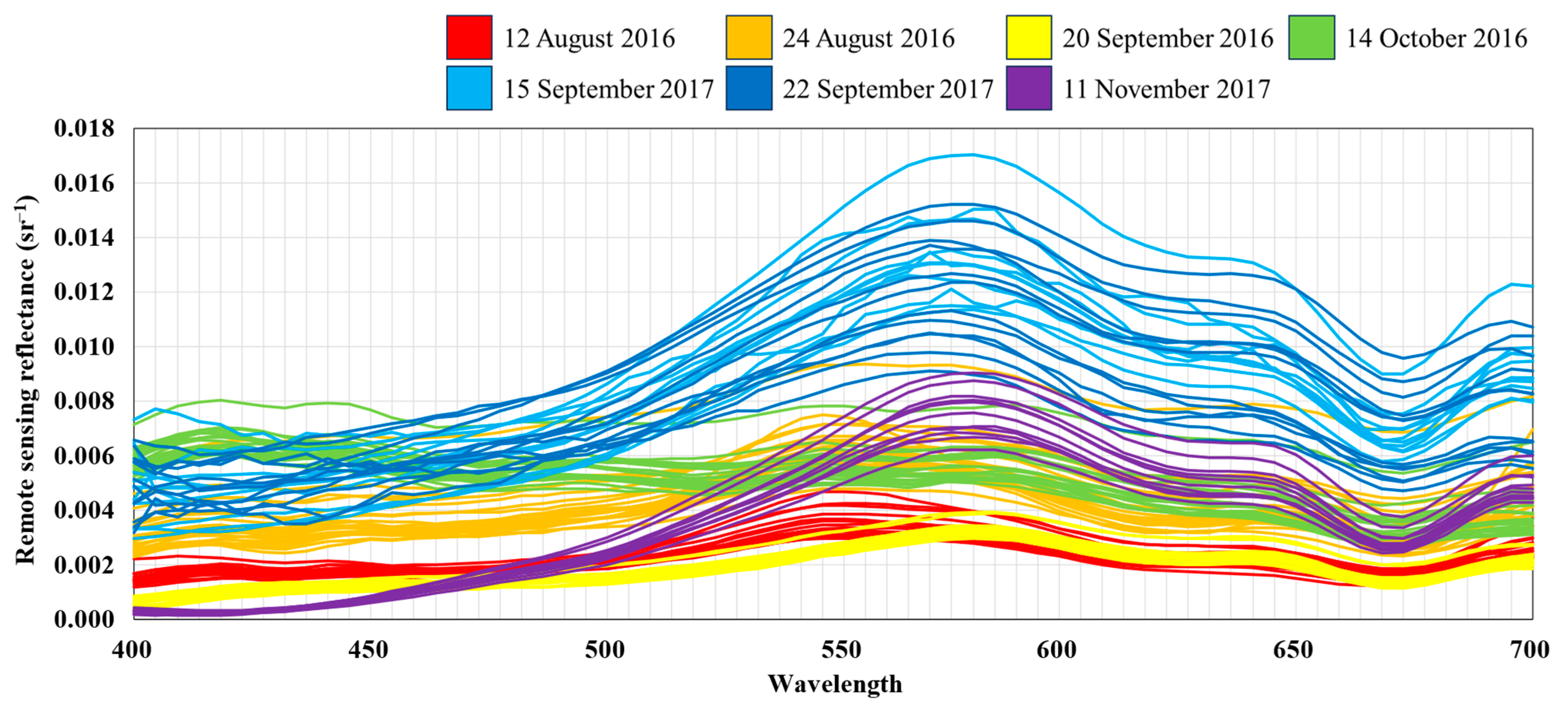
2.1.2. In Situ Reflectance Measurements and Airborne Hyperspectral Image

To monitor the BJR, hyperspectral imaging and water sampling from seven campaigns on four occasions in 2016 and three occasions in 2017 were conducted. For hyperspectral imaging, an AisaFENIX hyperspectral sensor (AISA Aero Survey Co., Ltd., Kawasaki, Japan) was used, which has a spectral resolution of 400–970 nm at 4–5 nm intervals and a spatial resolution of 2 m. The airborne campaigns were conducted for 2 to 3 h starting at 8:30 a.m. at an altitude of 3 km. Field sampling commenced at approximately 8:30 a.m. as well. Water sampling and in situ reflectance data were collected over a 3 h period at the monitoring stations. A total of 11–20 points were sampled for each monitoring event. The field reflectance for atmospheric correction was obtained using a FieldSpec Handheld2 spectroradiometer (ASD Inc., Boulder, CO, USA) in the wavelength range of 325–1075 nm. The MODTRAN code was developed at Science Inc. (Santa Monica, CA, USA), and the Air Force Research Laboratory was utilized to generate atmospheric correction parameters and subsequently calculate the surface reflectance of the hyperspectral images. The relationship between the atmospheric corrected reflectance and field reflectance through MODTRAN 6 presented in Pyo et al. [20] showed that the NSE was higher than 0.8 and the RMSE value was lower than 0.0034 sr⁻¹, and the parameter-related information is shown in Section A in the Supplementary Materials.

2.1.3. CDOM Absorption Coefficient

The CDOM absorption coefficient ($a_{CDOM}$) obtained from field monitoring was stored in polyvinyl chloride bottles under dark and refrigerated conditions before being transported to the laboratory. Upon arrival at the laboratory, the sample was filtered using a Millipore polycarbonate membrane (pore size = 0.22 um; $\mathsf{\Phi }$ = 45 mm). This membrane was pre-rinsed in a 10% HCl solution prior to filtering. The filtered solution was analyzed using a Cary 5000 UV-vis-NIR spectrophotometer (Agilent Technologies, Inc., Santa Clara, CA, USA). A 0.1 m quartz cuvette was used for the measurement. The absorption spectra were determined in the wavelength range of 350–800 nm at 1 nm intervals. The absorbance was converted into an absorption coefficient using Equation (1). To minimize the interference caused by light scattering, the average absorption at the highest end of the spectrum was subtracted and minimized, as shown in Equation (1) [21].

$$a_{CDOM}\left(\lambda \right)=2.303\times A\left(\lambda \right)/L$$

(1)

$${\alpha }_{\lambda }={\alpha }_{{\lambda }^{\prime }}-{\alpha }_{{avg\_range}^{\prime }}(\lambda /{\lambda }_{avg\_range})$$

(2)

where $A\left(\lambda \right)$ is the absorption of filtered water at a specific wavelength measured over the quartz cuvette path length $L$. ${\alpha }_{\lambda }$ is absorption coefficient at specific wavelength ($\lambda$) and the ${\lambda }_{avg\_range}$ was calculated considering an average absorption of 650–700 spectra [22]. Past studies have employed a range of wavelength intervals from 254 nm to 440 nm as reference wavelengths to characterize $a_{CDOM}$ in inland aquatic environments. Xu et al. [23] proposed 355 nm as the appropriate absorption coefficient for Poyang Lake after evaluating three wavelengths: 355 nm, 400 nm, and 440 nm. Kim et al. [24] assessed CDOM reference wavelengths ranging from 350 nm to 440 nm and concluded that the optimal performance was achieved within the range of 350~355 nm. Therefore, in this study, 355 nm was selected as the reference wavelength to quantify $a_{CDOM}\left(355\right)$ and was used as an output variable in the model.

Rainfall and runoff observation data from the BJR were used to understand the spatial distribution and trends of $a_{CDOM}$. Observation data were acquired from https://www.water.or.kr/ (accessed on 28 November 2023).

2.2. Feature Selection and Data Resampling Method

2.2.1. Feature Selection

The airborne hyperspectral image used as an input variable had 127 reflectance in the 400–970 nm range, but 66 bands in the 400–700 nm range of visible light were used. After imaging the entire BJR using a hyperspectral device mounted on an aircraft, atmospherically corrected reflectance values were obtained using MODTRAM 6. Figure 2 shows airborne hyperspectral values from 107 water sampling points from 12 August 2016 to 11 November 2017. Correlation analysis was performed to investigate the relationship between $a_{CDOM}\left(355\right)$ and single-band reflectance $R_{rs}$, and the final input variable was constructed by estimating the optimal value in the region of high correlation.

2.2.2. Data Resampling Method

Data resampling was used to solve the data imbalance problem. It comprises an undersampling technique that reduces the size of the majority class by deleting instances and an oversampling technique that adds new samples to the minority class. SMOTE is an oversampling technique that utilizes the k-NN algorithm to artificially generate new samples by respecting the distribution of minority classes. SMOTE operates on a “featurespace” rather than a “dataspace,” and the nearest neighbors are randomly selected along the line segments connecting some or all of the classes [25]. SMOTE defines neighbors for each element of the minority class, sets $k$ (usually five) close neighbors, and subsequently randomly selects $N<k$ elements and uses these elements to construct a new sample through interpolation. The synthetic sample is represented by Equation (3):

$$x_i^{*p}=x_i+u(x_i^p-x_i)$$

(3)

where a given sample $X_i$ is the data obtained from a minority class, and for a sample $X_i^p$ randomly selected from N neighbors; $p$ is 1,…; N refers to the synthetic sample $x_i^{*p}$; and $u$ is a randomly generated number between 0 and 1. SMOTE has the advantage of a fast calculation speed and provides balanced and accurate performance [26,27].

When generating synthetic data using SMOTE, a standard for dividing the data must exist. As the $a_{CDOM}\left(355\right)$ data were continuous, the distribution of the data was investigated in advance using a histogram to select the criteria for classification. Additionally, based on the results of the histogram and the literature review, a threshold for unbalanced data distribution was established, and the classes were divided based on this threshold to generate synthetic data for minority classes.

2.3. Construction of Machine Learning Models and Evaluation of Model Performance

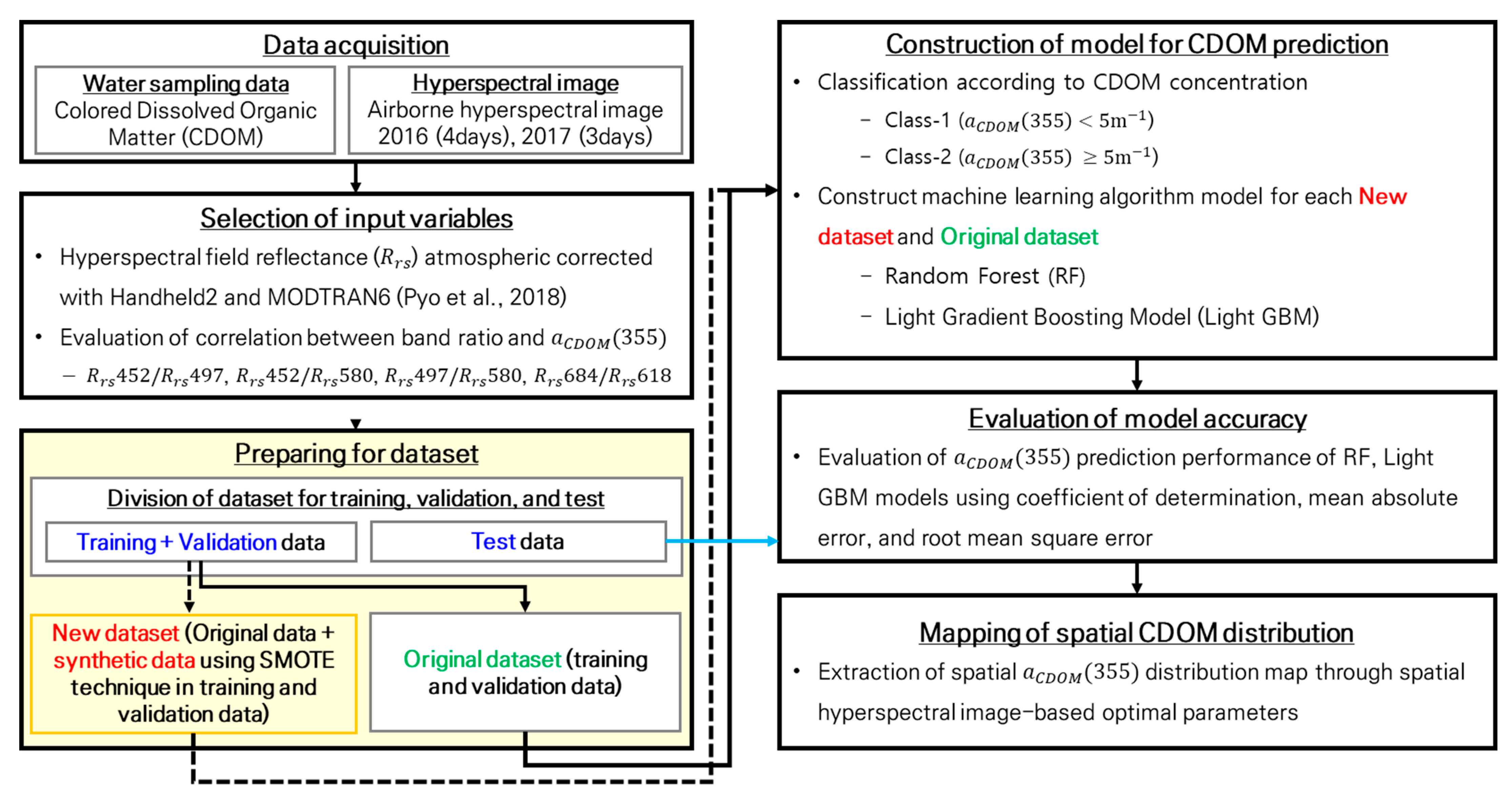
2.3.1. Model Process

Figure 3 shows a research flowchart of the model construction process. To introduce the SMOTE method, the training and testing data were first divided into a 75%:25% ratio for each class in the $a_{CDOM}\left(355\right)$ class and extracted through a histogram. An algorithm to quantify the nonlinear relationship between the reflectance ratio of the hyperspectral band and the absorption coefficient was constructed using random forest (RF) and light gradient boosting machine (LightGBM). RF and LightGBM were constructed for each of the new datasets that generated synthetic data by applying SMOTE to the training data and the original dataset that was not applied. The testing data were not included in this process and were subsequently calculated to verify the performances of the two algorithms.

2.3.2. Random Forest Algorithm

RF uses bootstrapping to generate $T$ random training sets S₁, S₂, … S_T. After that, a decision tree (ntree) is constructed, divided into several homogeneous subsets, and input variables are selected and classified so that homogeneity increases within the ntree and heterogeneity between ntrees, the prediction average for each tree is calculated to produce the model prediction result [16,28]. RF can relieve the overfitting problem of simple decision trees and is very powerful in including a large number of input variables. It also provides good accuracy even when there are missing items and heterogeneous variables [14]. RF is simpler than other machine learning models, but it shows better performance, and it presents a powerful algorithm, especially when the number of data is small, as in this study. Based on the previous study Kim et al. [24], $a_{CDOM}\left(355\right)$ prediction was performed through RF, and the performance of average R² 0.845 and average RMSE 0.68 m⁻¹ was inferred using variables of $R_{rs}\left(475\right)$, $R_{rs}\left(497\right)$, and $R_{rs}\left(660\right)$ in $a_{CDOM}\left(355\right)$.

The python sklearn random forest library was used, and the parameters used were “n_estimators”, “max_depth”, “max_features”, and “min_samples_split”. The “n_estimators” is the number of decision trees, and “max_depth” is the maximum depth of the tree. The “max_features” is the maximum number of features to consider for adversarial segmentation, and “min_samples_split” is the minimum number of sample data to split a node.

2.3.3. Light Gradient Boost Machine (Light GBM)

Light GBM is an ensemble tree-based machine learning algorithm featuring two functions: Gradient-Based One-Side Sampling (GOSS) and Exclusive Feature Bundling (EFB) based on GBDT (Gradient Boosting Decision Tree) [29]. GOSS selects a subset of the training data using the gradients of the loss function determined by the current model and EFB groups sparse features into dense features, thereby improving computer efficiency [30]. Light GBM employs the python lightgbm library, utilizing parameters such as “max_depth”, “num_leaves”, “bagging_fraction”, and “min_data_in_leaf”. The “max_depth” and “min_data_in_leaf” function similarly to “max_depth” and “min_samples_split” in RF. The “num_leaves” is the number of leaves in the entire tree, and “bagging_fraction” accelerates training and mitigates overfitting by selecting a portion of the data used for each iteration. The selected parameters were optimized using GridSearch to evaluate the performance of both the RF and Light GBM models constructed from all possible combinations.

2.3.4. Model Accuracy

The accuracy of the observed and simulated CDOM absorption coefficients was evaluated using the coefficient of determination (R²), absolute error (MAE), and root mean square error (RMSE). The equations used are as follows:

$$R^2={\left(\frac{{\sum }_{t=1}^T(C_{\mathrm{i}\mathrm{n}\mathrm{s}\mathrm{i}\mathrm{t}\mathrm{u}}^t-{\overline{C}}_{\mathrm{i}\mathrm{n}\mathrm{s}\mathrm{i}\mathrm{t}\mathrm{u}})(C_{\mathrm{a}\mathrm{l}\mathrm{g}\mathrm{o}\mathrm{r}\mathrm{t}\mathrm{h}\mathrm{i}\mathrm{m}}^t-{\overline{C}}_{\mathrm{a}\mathrm{l}\mathrm{g}\mathrm{o}\mathrm{r}\mathrm{t}\mathrm{h}\mathrm{i}\mathrm{m}})}{\sqrt{{\sum }_{t=1}^T(C_{\mathrm{i}\mathrm{n}\mathrm{s}\mathrm{i}\mathrm{t}\mathrm{u}}^t-{\overline{C}}_{\mathrm{i}\mathrm{n}\mathrm{s}\mathrm{i}\mathrm{t}\mathrm{u}})}\sqrt{{\sum }_{t=1}^T(C_{\mathrm{a}\mathrm{l}\mathrm{g}\mathrm{o}\mathrm{r}\mathrm{t}\mathrm{h}\mathrm{i}\mathrm{m}}^t-{\overline{C}}_{\mathrm{a}\mathrm{l}\mathrm{g}\mathrm{o}\mathrm{r}\mathrm{t}\mathrm{h}\mathrm{i}\mathrm{m}})}}\right)}^2$$

(4)

$$MAE=\frac{{\sum }_{t=1}^T\left|C_{\mathrm{a}\mathrm{l}\mathrm{g}\mathrm{o}\mathrm{r}\mathrm{i}\mathrm{t}\mathrm{h}\mathrm{m}}^t-C_{\mathrm{i}\mathrm{n}\mathrm{s}\mathrm{i}\mathrm{t}\mathrm{u}}^t\right|}{n}$$

(5)

$$RMSE=\sqrt{\frac{{\sum }_{t=1}^T{\left(C_{\mathrm{a}\mathrm{l}\mathrm{g}\mathrm{o}\mathrm{r}\mathrm{i}\mathrm{t}\mathrm{h}\mathrm{m}}^t-C_{\mathrm{i}\mathrm{n}\mathrm{s}\mathrm{i}\mathrm{t}\mathrm{u}}^t\right)}^2}{n}}$$

(6)

where $T$ denotes the number of samples; $C_{\mathrm{i}\mathrm{n}\mathrm{s}\mathrm{i}\mathrm{t}\mathrm{u}}$ is the observed $a_{CDOM}$ in situ; and $C_{\mathrm{a}\mathrm{l}\mathrm{g}\mathrm{o}\mathrm{r}\mathrm{t}\mathrm{h}\mathrm{i}\mathrm{m}}$ is the estimated $a_{CDOM}$ using the RF and Light GBM models.

After evaluating the accuracy, the CDOM distribution in the BJR was confirmed using the CDOM spatial distribution map based on the original and new datasets in the optimal-case scenario. Data analysis, model construction, and evaluation were performed using Python software, version 3.7.

3. Results

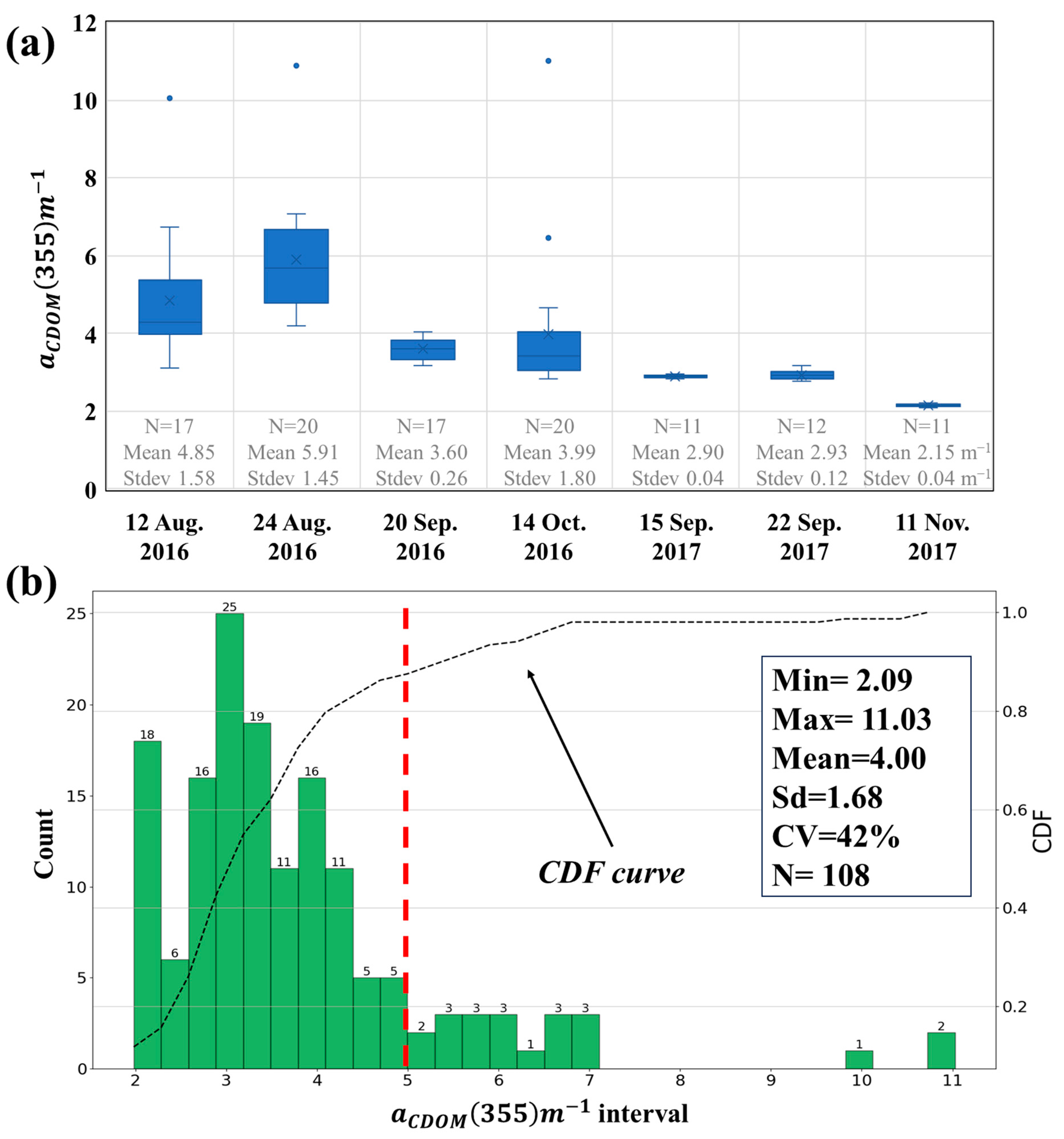
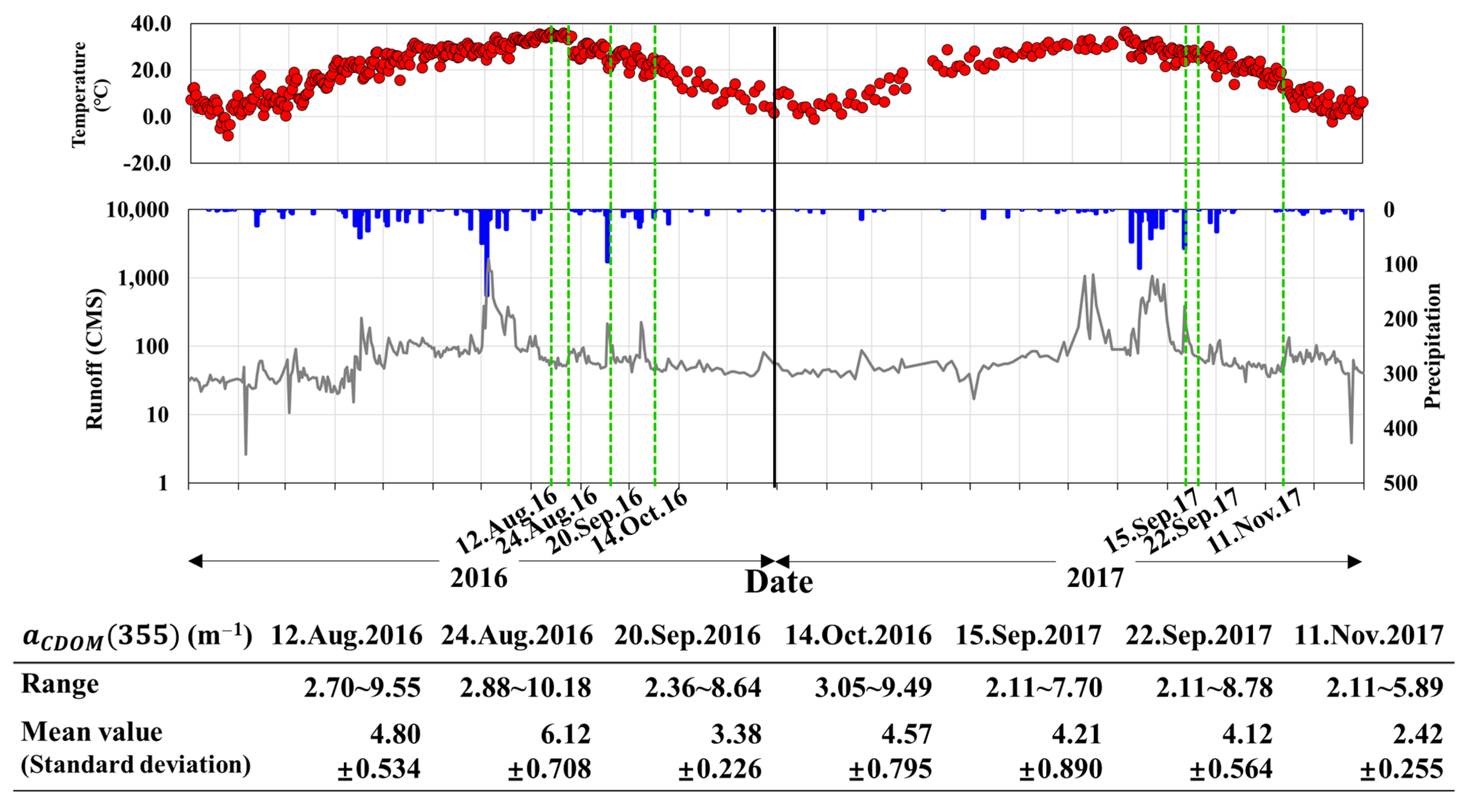
3.1. Descriptive Analysis of Chromophoric Dissolved Organic Matter (CDOM) in Reservoirs

The $a_{CDOM}\left(355\right)$ data obtained via field sampling are shown in Figure 4. There was a total of 108 $a_{CDOM}\left(355\right)$ data points, consisting of 74 in 2016 and 34 in 2017, and the distribution of daily $a_{CDOM}\left(355\right)$ is expressed as a boxplot in Figure 4a. $a_{CDOM}\left(355\right)$ for the 2016 data was highly dynamic, with 3.12–10.05 m⁻¹ on 12 August 2016, 4.19–10.88 m⁻¹ on 24 August 2016, and 2.83–11.03 m⁻¹ on 14 October 2016. The ranges are shown, and the coefficients of variation were 33%, 25%, and 45%, respectively, indicating significant variability. Conversely, on 20 September 2016, and 15 September, 22 September, and 11 November 2017, the average values were 3.60 m⁻¹, 2.90 m⁻¹, 2.93 m⁻¹, and 2.15 m⁻¹, respectively, and the standard deviations were 0.26 m⁻¹, 0.04 m⁻¹, 0.12 m⁻¹, and 0.04 m⁻¹, respectively, indicating a coefficient of variation between 1 and 7%.

Figure 4b shows the histogram and cumulative distribution functions of the total $a_{CDOM}\left(355\right)$ data. The minimum and maximum value range, 2.09–11.03 m⁻¹, was divided into 20 sections, and a histogram including the number of samples in each section is illustrated. Most of these sections were in the range of −4 m⁻¹, and the probability density up to 4 m⁻¹ was 80.0%. We set 5 m⁻¹, which corresponded to half of the section, excluding the missing section, as the standard value for dividing the high- and low-concentration classes. $a_{CDOM}\left(355\right)$ values less than 5 m⁻¹ were placed in Class 1, which was a low-concentration range, and values over 5 m⁻¹ were placed in Class 2, which was a high-concentration range. The probability of Class 2 was approximately 13.4%, and the number was 20.

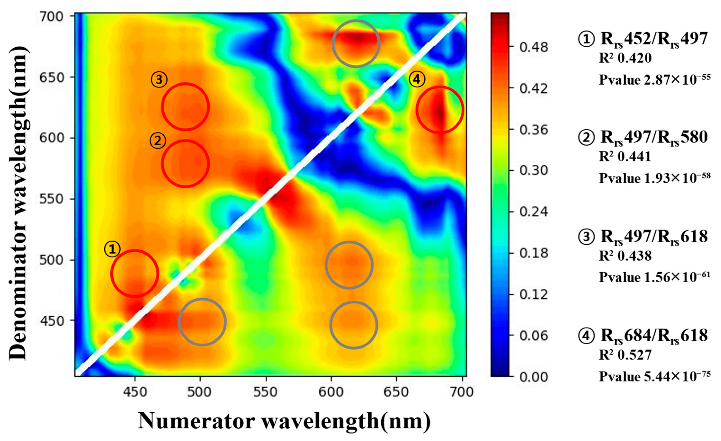
3.2. Results of Feature Selection

Correlation analysis was performed to investigate the relationship between CDOM and the band reflectance ratio $R_{rs}$ in the spectral range of 400–700 nm. In Figure 5, the R² values between $a_{CDOM}\left(355\right)$ and the numerator/denominator reflectance ratio are shown as a heatmap; the higher the R² value, the redder it appears. The discrepancy in wavelength between the two spectral bands was fixed at 40 nm to minimize errors in field measurements and to facilitate their utilization in multispectral remote sensing imagery via satellite imaging [23]. Furthermore, in cases where identical reflectance ratios are present (e.g., $R_{rs}(684/618)$ and $R_{rs}(618/684)$), only the higher value was chosen, regardless of both exhibiting high R² values. The chosen ratios consisted of $R_{rs}(452/497)$, $R_{rs}(497/580)$, $R_{rs}(497/618)$, and $R_{rs}(684/618)$, exhibiting significant R² values (p-values < 0.05) ranging from 0.408 to 0.527.

3.3. Comparison of Machine Learning Model Performance

The $a_{CDOM}\left(355\right)$ data with reflectance were divided into training and testing sets for each class at a ratio of 75%:25%, respectively. The original dataset was constructed using the training data, and a new dataset was constructed using the training and synthetic data generated using the SMOTE method. RF and Light GBM models were constructed by targeting the original and new datasets, and the overall performance was evaluated by iteratively running the model 200 times. The RF tested hyperparameters included the number of trees within the range of 10–100; the maximum number of features calculated using the auto, sqrt, and log2 methods based on the number of data provided by the Python RandomForestRegressor library; the maximum depth of the tree within the range of 2–20; and the minimum number of sample data points within the range of 2–10. Light GBM hyperparameters were tested in the range of “max_depth” from 2 to 10, “num_leaves” from 8 to 200, “min_data_in_leaf” from 3 to 10, and “bagging_fraction” from 0.5 to 1.0.

Table 1. Comparison of overall performance of random forest and light gradient boosting machine considering original data and new data using the synthetic minority oversampling technique (SMOTE) method.

Model	Method	Train R2	Test R2	Train MAE	Test MAE	Train RMSE	Test RMSE
Random Forest	Original	0.645	0.500	0.645	0.716	1.076	1.012
		(±0.116)	(±0.132)	(±0.129)	(±0.141)	(±0.182)	(±0.223)
	SMOTE	0.798	0.476	0.620	0.880	0.984	1.338
		(±0.127)	(±0.148)	(±0.219)	(±0.202)	(±0.300)	(±0.325)
Light Gradient Boosting Machine	Original	0.618	0.564	0.757	0.697	1.252	0.882
		(±0.077)	(±0.135)	(±0.086)	(±0.096)	(±0.108)	(±0.134)
	SMOTE	0.844	0.456	0.569	0.907	0.893	1.357
		(±0.088)	(±0.161)	(±0.220)	(±0.203)	(±0.332)	(±0.341)

displays the overall performance scenario for RF and Light GBM selected based on the R², MAE, and RMSE metrics. The overall training of RF showed that the SMOTE R² was 0.798, which was 0.152 higher than that of the original. Moreover, the MAE and RMSE were 0.620 and 0.984 m⁻¹, respectively, which were 0.025 and 0.092 m⁻¹ lower than those of the original, respectively. For the test performance, the original R² was 0.500, which was 0.024 higher than that of SMOTE. The MAE and RMSE were 0.716 and 1.012 m⁻¹, respectively, which were 0.164 and 0.326 m⁻¹ lower than those of SMOTE, respectively. In the overall training of Light GBM, SMOTE R² was 0.844, which was 0.226 higher than the original R². The test R² was 0.456, which was 0.108 lower than the original R², but the standard deviation was larger at 0.161. In other words, when SMOTE was applied, the fit in the training process was higher, and the accuracy in the testing process was more clearly distributed than in the original. Within the model, when SMOTE was applied, the training R² of Light GBM was higher than that of RF, whereas the test R² of RF was higher than that of Light GBM. The training MAE and RMSE of Light GBM were lower than those of RF, whereas the test MAE and RMSE of RF were lower than those of Light GBM.

The best case was selected based on the R², MAE, and RMSE (

Table 2. Comparison of the best-case performance of random forest and light gradient boosting machine by each model accuracy (R², MAE, RMSE) considering original data and new data using the synthetic minority oversampling technique (SMOTE) method.

Model	Method	Model Accuracy	Train R2	Test R2	Train MAE	Test MAE	Train RMSE	Test RMSE
Random Forest	Original	R2	0.823	0.722	0.433	0.493	0.756	0.802
		MAE/RMSE	0.900	0.628	0.341	0.556	0.604	0.830
	SMOTE	R2	0.898	0.838	0.471	0.566	0.765	0.777
		MAE/RMSE	0.881	0.816	0.468	0.495	0.793	0.682
Light Gradient Boosting Machine	Original	R2	0.945	0.583	0.590	0.691	0.906	0.867
		MAE	0.738	0.628	0.341	0.556	0.604	0.830
		RMSE	0.813	0.571	0.459	0.599	0.881	0.881
	SMOTE	R2/MAE/RMSE	0.993	0.772	0.142	0.531	0.225	0.837

). The average train and test R² of RF was 0.773 with the original method and 0.868 with SMOTE, while the average train and test R² of Light GBM was 0.764 with the original method and 0.883 with SMOTE. The R² values for both models in the training and test steps increased when SMOTE was applied. Although the performance of Light GBM with SMOTE remained consistent across various evaluation metrics, its training R² was excessively high at 0.993 and its test R² was relatively low at 0.772 compared to test R² of 0.838 for the RF model. Thus, the RF model showed better generalization performance than Light GBM.

Figure 6 and Figure S1 show the results of the best-case scenario for RF and Light GBM, illustrating a comparison between simulated and observed $a_{CDOM}\left(355\right)$ values; low-concentration (Class 1) and high-concentration (Class 2) prediction accuracy were based on 5 m⁻¹ without any distinction between training and testing datasets. Data synthesized with SMOTE were mainly interpolated between 5 and 10 m⁻¹ in Class 2, and high-concentration data above 10 m⁻¹ increased from 3 to 6–8. For the cases shown in Figure 6c,g, which were selected as R², the Class 1 R² was 0.696 and 0.741, respectively, and the Class 2 R² was 0.606 and 0.691, respectively, thereby showing relatively poor performance compared to the predicted values. In contrast, in Figure 6d,h, selected by MAE/RMSE, the Class 1 R² was high at 0.709 and 0.684, respectively, and the Class 2 R² was high at 0.787 and 0.839, respectively. In addition, when SMOTE was applied to the values selected as MAE/RMSE, the MAE and RMSE were 0.485 and 0.712 m⁻¹ in Class 2, respectively, which were 0.172 and 0.265 m⁻¹ lower than the original values, respectively. In addition, the trend in the graph appeared to improve in some areas that were somewhat underestimated. Finally, based on the MAE/RMSE, Figure 6b was selected from the original dataset, and Figure 6d was selected from the new dataset, where SMOTE was calculated and the spatial distribution was performed. The optimal hyperparameters for “n_estimators”, “max_depth”, “max_features”, and “min_samples_split” were 10, 8, log2, and 2, respectively, in the original dataset and 10, 16, log2, and 4, respectively, in the new dataset. The description of the Light GBM results was provided in Section B of the Supplementary Materials.

3.4. Analysis of CDOM High-Concentration Distribution Area

Figure 7 exhibits the CDOM spatial distribution results when the original and new dataset-based RF model were applied. This shows the spatial distribution of areas with relatively high values within the concentration ranges. For points in Figure 7a,g, the observed $a_{CDOM}\left(355\right)$ values were 10.1 m⁻¹ and 11.1 m⁻¹, respectively, and the result values predicted from the spatial distribution were 8.1 m⁻¹ and 8.2 m⁻¹, respectively, based on the original data. SMOTE yielded values of 7.6 m⁻¹ and 9.4 m⁻¹. The area section on 12 August 2016, showed a spatial range of 2.8–8.1 m⁻¹ based on the original dataset and a spatial range of 2.9–7.7 m⁻¹ based on the SMOTE dataset. The area section on 14 October 2016, showed a spatial range of 3.0–8.2 m⁻¹ based on the original dataset and 3.1–9.3 m⁻¹ based on the SMOTE dataset. The observed values were higher in the section measured at the waterside than at the center of the river. Conversely, 24 August 2016 had a value of 10.9 m⁻¹, and the original and SMOTE values were 8.8 m⁻¹ and 9.8 m⁻¹, respectively. The spatial area value ranged from 4.3 to 9.9 m⁻¹ in the original and 4.2 to 10.2 m⁻¹ in SMOTE, and the spatial average value was 6.0 (±0.62) m⁻¹ in the original and 7.0 (±0.83) m⁻¹ in SMOTE. This analysis appeared to provide a better understanding of the high concentrations in the central part of the river center and along the waterside.

4. Discussion

4.1. Selection of Input Variables

To predict $a_{CDOM}\left(355\right)$, the highest R² value was selected from the reflectance ratio through hyperspectral images, and $R_{rs}$452/$R_{rs}$497, $R_{rs}$497/$R_{rs}$580, $R_{rs}$497/$R_{rs}$618, and $R_{rs}$684/$R_{rs}$618 were used in this study. CDOM absorbs light in the range of 480–510 nm and weakly absorbs light in the range of 660–700 nm. In water, where CDOM was suspended, more blue and green light was absorbed than red light; therefore, more red light can be reflected into the atmosphere. Wavelengths greater than 600 nm are important for accurately estimating CDOM in complex freshwater ecosystems [13,31]. In this study, R² values for input selection in $R_{rs}$684/$R_{rs}$618, $R_{rs}$497/$R_{rs}$580, and $R_{rs}$497/$R_{rs}$618, which included reflectance in the green and red regions, were the highest at 0.527, 0.441, and 0.438, respectively. Notably, numerous studies have also used reflectance that includes the green–red ratio [3,13,32].

The blue band has the strongest aerosol scattering, causing problems with atmospheric correction, and was not mainly used in CDOM retrieval even though it is the area where the optical characteristics of CDOM are best revealed [33]. Nevertheless, in this study, a stronger correlation appears than other wavelength ratios around 490 nm, which is the standard for the diffuse attenuation coefficient for downward irradiance, and 443 nm, which is the reference wavelength of CDOM. This blue band is also utilized through QAA analysis and the Carder algorithm of Lee et al. [34], Zhu et al. [35], Carder et al. [36], and the IOCCG [37], and is used in CDOM retrieval through its relationship with 580 nm. Reflectance above 700 nm was not selected because there is no absorption of CDOM, for CDOM retrieval. Recent studies point out that near infrared radiation (NIR) bands were generally useful for easy separation of CDOM in turbid and eutrophic regions [23,38,39]. This is because the lowest absorption point of pure water occurs at 770 nm to 850 nm, and as eutrophication occurs, the backscattering coefficient increases and the reflection spectrum in NIR is affected [40,41].

4.2. Evaluation of Machine Learning Models and Application of Data Resampling

A small dataset of 108 data points was used in this study. SMOTE, a data resampling method, was applied to resolve the data imbalance in high and low concentrations of CDOM and to increase the number of data in the training step. The CDOM prediction performance of the RF and Light GBM models trained using a dataset with added synthetic data generated by SMOTE was reasonable. The Light GBM model showed a tendency of overfitting in the training step, compared to the RF model in the best-case scenario because the test performance of the RF model was higher than that of Light GBM. The optimal model for CDOM prediction was selected as RF, considering all performance indices and overfitting problems. RF can reduce data variance in small datasets and prevent dependence on highly influential variables. RF can reduce the impact of overfitting values and outliers compared to artificial neural networks or deep learning and generate more accurate predictions than other algorithms, especially when there is an imbalanced class in the dataset [42,43].

Data resampling techniques are widely used for classification problems. To apply the data resampling technique to the regression problem, we created a histogram of the distribution of $a_{CDOM}\left(355\right)$ and established a threshold to differentiate between high and low concentrations. After constructing the synthetic data for low (Class 1) and high concentrations (Class 2) based on the threshold, the RF algorithm was applied. Consequently, the average R² and MAE of the training and testing values in the best-case scenario increased by 0.096 and 0.056, respectively, and the RMSE decreased by 0.008 compared with those that were not applied. The total number of CDOM data points generated in the best-case scenario was 47. When combined with 17 Class 2 data points, the same number of $a_{CDOM}\left(355\right)$ data points were generated as in Class 1. The $a_{CDOM}\left(355\right)$ value significantly interpolated the imbalanced data in the high-concentration section, as shown in Figure 8.

In this study, the threshold for distinguishing between low and high $a_{CDOM}\left(355\right)$ was determined through statistical methods. The threshold identified in this research was 5 m⁻¹, which proved to be a reasonable outcome in comparison to findings from prior research. Brezonik et al. [7] noted that regions with a440 values exceeding 5 m⁻¹ were dominated by allochthonous (humic-rich) sources, while lower values were influenced by autochthonous sources, highlighting distinct characteristics between the two reservoirs. Meler et al. [44] reconstructed the $a_{CDOM}\left(355\right)$ algorithm to incorporate high-concentration data based on a threshold of 5 m⁻¹ using a Baltic Sea dataset. Jiang et al. [11] observed that $a_{CDOM}\left(375\right)$ values were predominantly distributed within the range of 0~5 m⁻¹ and displayed limited sensitivity to the algorithm above 5 m⁻¹. Consequently, multiple studies have yielded results aligning closely with our threshold value.

Data imbalance problems can be solved by using models, and there is also a way to utilize the data themselves. In the classification model, various machine learning techniques such as extreme gradient boost and light gradient boosting machine have already been introduced to solve the data imbalance problem using parameters such as class_weight [45]. For the data approach, when the amount of data is sufficiently supplemented, an undersampling technique can be applied to remove samples from the majority class until there is a balance between the minority and majority classes. In addition, a hybrid sampling method that combines oversampling and undersampling can be proposed. Chandra et al. [46] employed the SMOTE-TOMEK technique to solve the imbalance problem of air quality index data, and Kim et al. [47] used SMOTE-edited nearest neighbor (SMOTE-ENN), a hybrid sampling method. The alert levels for high algal concentrations were predicted using this method. In the field of remote sensing, Wen et al. [48] recently processed imbalanced data on a large scale using a method combining SMOTE and Gaussian noise to predict suspended particulate matter (SPM) concentrations based on Landsat images; the results of RF improved from R² = 0.46 and RMSE = 18.8 to R² = 0.73 and RMSE = 14.1 in Chagan Lake.

4.3. Spatial Distribution Results

In Figure 9, rainfall, temperature, and discharge in the BJR station are compared to determine the spatial distribution trend of the high-concentration section, and the sampling date are indicated. In addition, the range, average, and standard deviation of $a_{CDOM}\left(355\right)$ in the entire BJR section are shown in a table. Prior to 12 August 2016, rainfall of 17.5 mm and 4.5 mm occurred on August 2 and August 6, respectively. Subsequent to August 6, a high value of $a_{CDOM}\left(355\right)$ was observed near the BJR, where organic matter was deposited due to a runoff of less than 100 CMS. It is judged that deteriorating values appear in the riverside from the waterside area, and the overall $a_{CDOM}\left(355\right)$ range is wide, ranging from 2.70 m⁻¹ to 9.55 m⁻¹. There was no rainfall between August 6 and August 24. The discharge was limited at 36.1–87.2 CMS, and high temperatures of 34–36.2 °C persisted during this period, resulting in a high $a_{CDOM}\left(355\right)$. On October 14, 2016, it was observed that the $a_{CDOM}\left(355\right)$ at the waterside increased due to a low runoff of 47.5–63.5 CMS from October 11 following 21.5 mm of rainfall on October 8. The $a_{CDOM}\left(355\right)$ was the highest when the Chl-a bloom collapsed, and high residual amounts appeared. Furthermore, there was a delay between the peak values of Chl-a and $a_{CDOM}\left(355\right)$ [49]. This explains why CDOM showed the highest distribution on August 24, which differed from previous studies [20,50] where Chl-a was highest on August 12.

5. Conclusions

In this study, we examined a CDOM prediction model by employing random forest (RF) and light gradient boosting machine (Light GBM) and the SMOTE method to solve the data imbalance problem at high concentrations and increase prediction accuracy. To select the input variables, the reflectance extracted through atmospheric correction from the hyperspectral image was used, and the highest R² value was applied through a band ratio heatmap. The main conclusions of this study are as follows:

• The selected input values that considered the overlap in the reflectance ratio R² heatmap of the hyperspectral images were $R_{rs}(452/497)$, $R_{rs}(497/580)$, $R_{rs}(497/618)$, and $R_{rs}(684/618)$ with R² values of 0.420, 0.441, 0.438, and 0.527, respectively. The machine learning models were constructed using the four input variables with significant p-values.
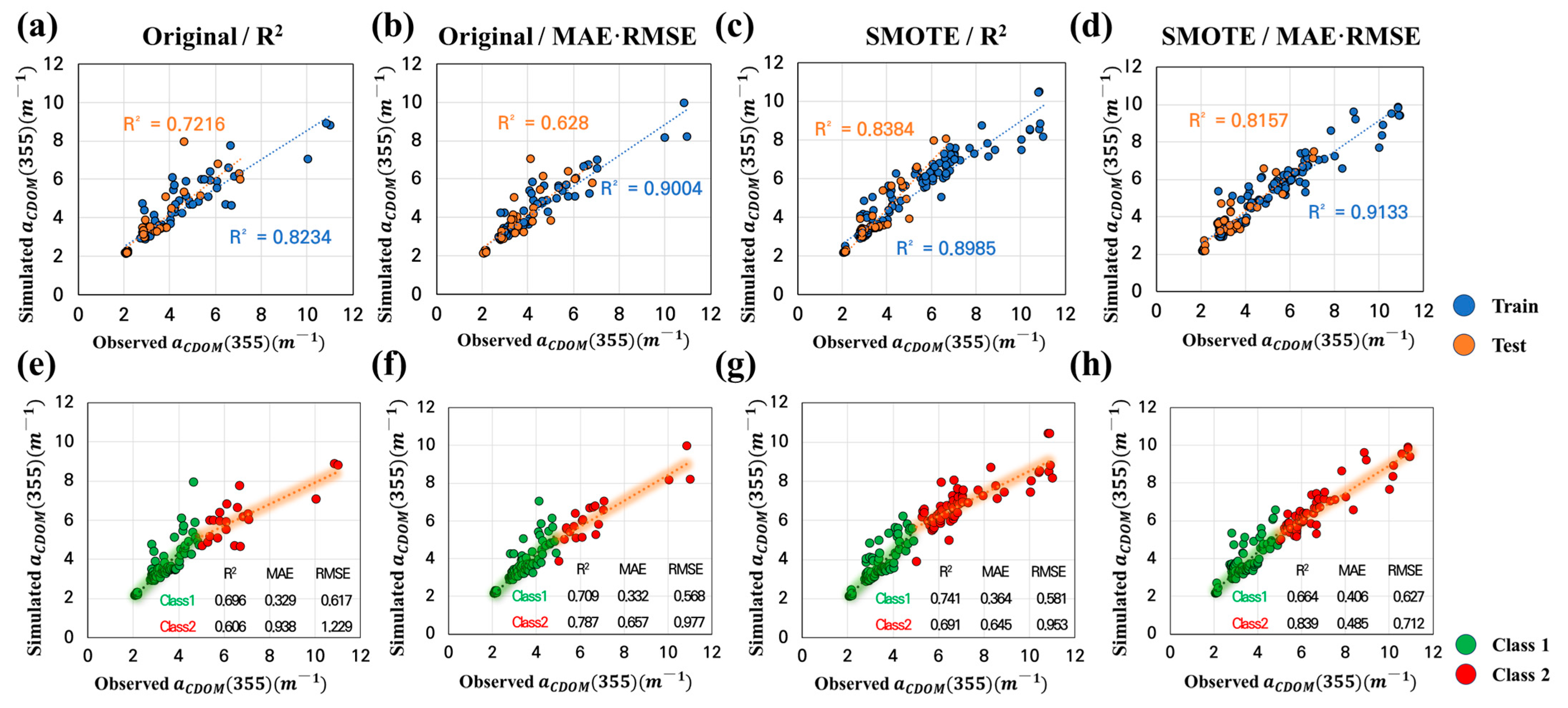
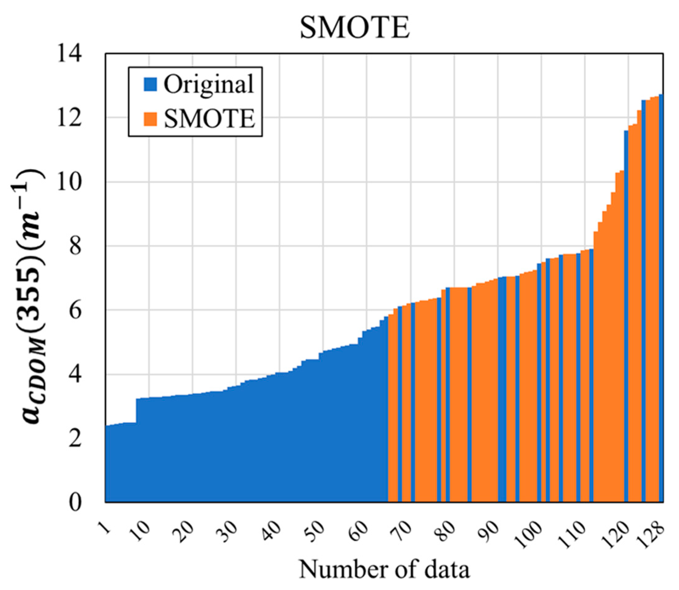
• To solve the imbalance problem, low-concentration (Class 1) and high-concentration (Class 2) sections were separated by 5 m⁻¹ in the small CDOM dataset, and training and testing datasets for each class were extracted. The training data were divided into two subsets: the original dataset, which used only the training data, and the SMOTE dataset, in which SMOTE was applied to the training dataset. The machine learning models were constructed and evaluated for each dataset to compare the CDOM prediction performance of the original and SMOTE datasets.
• Both RF and Light GBM demonstrated considerable performance improvements in the best-case scenario when SMOTE was applied. The R² values of RF were 0.881 and 0.816 in the training and test steps, whereas the R² values of Light GBM were 0.993 and 0.772 in the training and test steps. The RF model showed better generalization performance than Light GBM.
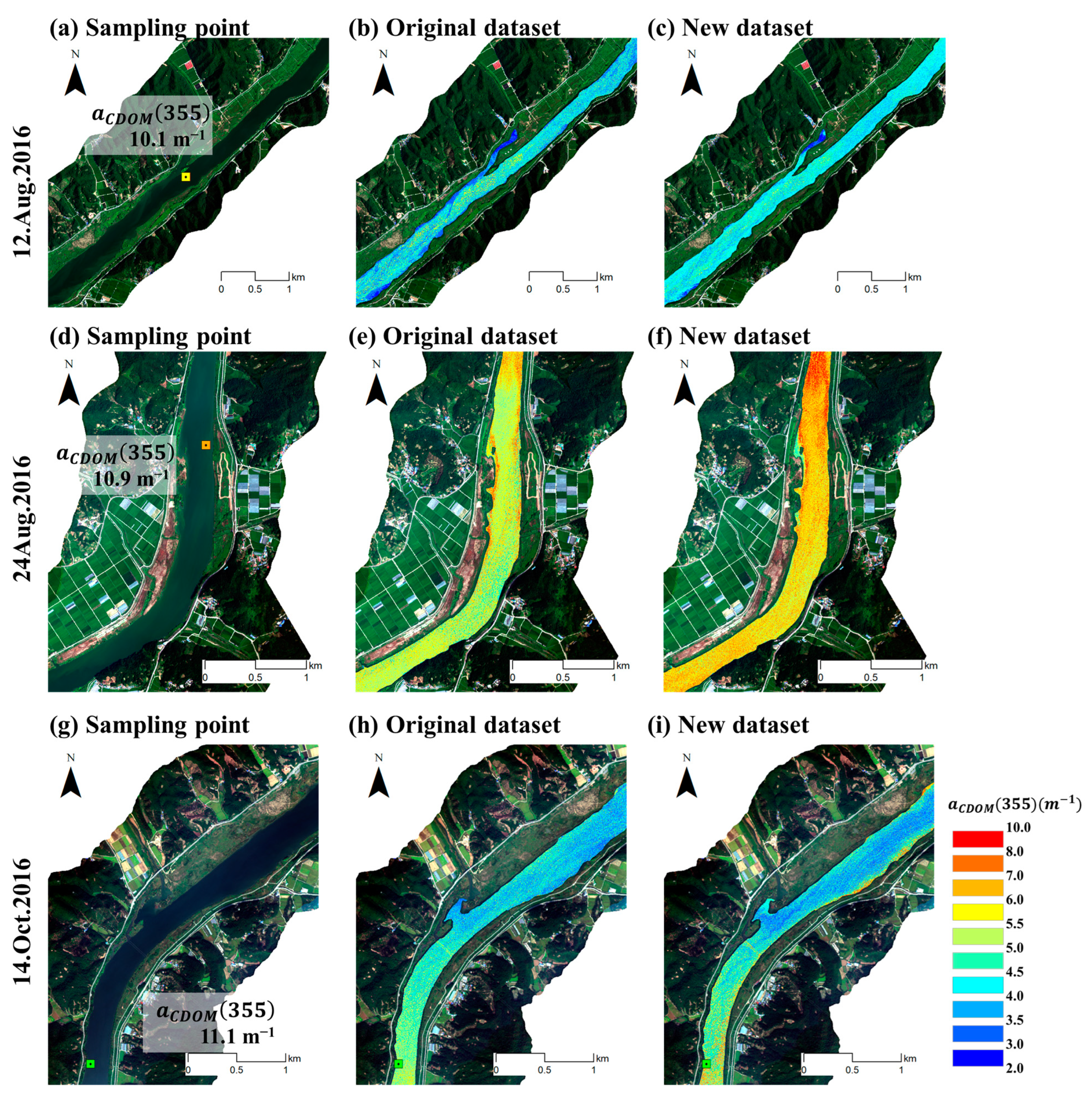
• Spatial distribution was performed using the results of this study, and it was confirmed that the SMOTE dataset detected CDOM on high-concentration days more accurately than the original dataset.

Based on the results of this study, it is possible to solve the data imbalance problem and improve the prediction accuracy when the CDOM dataset is small. This will also aid in the accurate estimation of reservoir water quality monitoring, which is crucial for water resource management.

References

1. Kirk, J.T.O. Light and Photosynthesis in Aquatic Ecosystems; Cambridge University Press: Cambridge, UK, 1994; ISBN 9788578110796. [Google Scholar]
2. Zhao, Y.; Song, K.; Wen, Z.; Li, L.; Zang, S.; Shao, T.; Li, S.; Du, J. Seasonal Characterization of CDOM for Lakes in Semiarid Regions of Northeast China Using Excitation–Emission Matrix Fluorescence and Parallel Factor Analysis (EEM–PARAFAC). Biogeosciences 2016, 13, 1635–1645. [Google Scholar] [CrossRef]
3. Kutser, T.; Pierson, D.C.; Kallio, K.Y.; Reinart, A.; Sobek, S. Mapping Lake CDOM by Satellite Remote Sensing. Remote Sens. Environ. 2005, 94, 535–540. [Google Scholar] [CrossRef]
4. Coble, P.G. Marine Optical Biogeochemistry: The Chemistry of Ocean Color. Chem. Rev. 2007, 107, 402–418. [Google Scholar] [CrossRef]
5. Ling, Z.; Sun, D.; Wang, S.; Qiu, Z.; Huan, Y.; Mao, Z.; He, Y. Remote Sensing Estimation of Colored Dissolved Organic Matter (CDOM) from GOCI Measurements in the Bohai Sea and Yellow Sea. Environ. Sci. Pollut. Res. 2020, 27, 6872–6885. [Google Scholar] [CrossRef] [PubMed]
6. Menken, K.D.; Brezonik, P.L.; Bauer, M.E. Influence of Chlorophyll and Colored Dissolved Organic Matter (CDOM) on Lake Reflectance Spectra: Implications for Measuring Lake Properties by Remote Sensing. Lake Reserv. Manag. 2006, 22, 179–190. [Google Scholar] [CrossRef]
7. Brezonik, P.L.; Olmanson, L.G.; Finlay, J.C.; Bauer, M.E. Factors Affecting the Measurement of CDOM by Remote Sensing of Optically Complex Inland Waters. Remote Sens. Environ. 2015, 157, 199–215. [Google Scholar] [CrossRef]
8. Griffin, C.G.; Frey, K.E.; Rogan, J.; Holmes, R.M. Spatial and Interannual Variability of Dissolved Organic Matter in the Kolyma River, East Siberia, Observed Using Satellite Imagery. J. Geophys. Res. Biogeosciences 2011, 116, 1–12. [Google Scholar] [CrossRef]
9. De Almeida, C.S.; Miccoli, L.S.; Andhini, N.F.; Aranha, S.; de Oliveira, L.C.; Artigo, C.E.; Em, A.A.R.; Em, A.A.R.; Bachman, L.; Chick, K.; et al. Remote Sensing of Ocean Colour in Coastal, and Other Optically-Complex, Waters; International Ocean Colour Coordinating Group (IOCCG): Dartmouth, NS, Canada, 2000; Volume 3. [Google Scholar]
10. Zhang, H.; Yao, B.; Wang, S.; Wang, G. Remote Sensing Estimation of the Concentration and Sources of Coloured Dissolved Organic Matter Based on MODIS: A Case Study of Erhai Lake. Ecol. Indic. 2021, 131, 108180. [Google Scholar] [CrossRef]
11. Jiang, G.; Ma, R.; Duan, H.; Loiselle, S.A.; Xu, J.; Liu, D. Remote Determination of Chromophoric Dissolved Organic Matter in Lakes, China. Int. J. Digit. Earth 2014, 7, 897–915. [Google Scholar] [CrossRef]
12. Zhu, W.; Yu, Q. Inversion of Chromophoric Dissolved Organic Matter from EO-1 Hyperion Imagery for Turbid Estuarine and Coastal Waters. IEEE Trans. Geosci. Remote Sens. 2013, 51, 3286–3298. [Google Scholar] [CrossRef]
13. Zhu, W.; Yu, Q.; Tian, Y.Q.; Becker, B.L.; Zheng, T.; Carrick, H.J. An Assessment of Remote Sensing Algorithms for Colored Dissolved Organic Matter in Complex Freshwater Environments. Remote Sens. Environ. 2014, 140, 766–778. [Google Scholar] [CrossRef]
14. Ruescas, A.B.; Hieronymi, M.; Mateo-Garcia, G.; Koponen, S.; Kallio, K.; Camps-Valls, G. Machine Learning Regression Approaches for Colored Dissolved Organic Matter (CDOM) Retrieval with S2-MSI and S3-OLCI Simulated Data. Remote Sens. 2018, 10, 786. [Google Scholar] [CrossRef]
15. Keller, S.; Maier, P.M.; Riese, F.M.; Norra, S.; Holbach, A.; Börsig, N.; Wilhelms, A.; Moldaenke, C.; Zaake, A.; Hinz, S. Hyperspectral Data and Machine Learning for Estimating CDOM, Chlorophyll a, Diatoms, Green Algae and Turbidity. Int. J. Environ. Res. Public Health 2018, 15, 1881. [Google Scholar] [CrossRef] [PubMed]
16. Sun, X.; Zhang, Y.; Zhang, Y.; Shi, K.; Zhou, Y.; Li, N. Machine Learning Algorithms for Chromophoric Dissolved Organic Matter (Cdom) Estimation Based on Landsat 8 Images. Remote Sens. 2021, 13, 3560. [Google Scholar] [CrossRef]
17. Chawla, N.V.; Japkowicz, N.; Kotcz, A. Editorial: Special issue on learning from imbalanced data sets. ACM SIGKDD Explor. Newsl. 2004, 6, 1–6. [Google Scholar] [CrossRef]
18. Bourel, M.; Segura, A.M.; Crisci, C.; López, G.; Sampognaro, L.; Vidal, V.; Kruk, C.; Piccini, C.; Perera, G. Machine Learning Methods for Imbalanced Data Set for Prediction of Faecal Contamination in Beach Waters. Water Res. 2021, 202, 117450. [Google Scholar] [CrossRef] [PubMed]
19. Kim, J.H.; Shin, J.K.; Lee, H.; Lee, D.H.; Kang, J.H.; Cho, K.H.; Lee, Y.G.; Chon, K.; Baek, S.S.; Park, Y. Improving the Performance of Machine Learning Models for Early Warning of Harmful Algal Blooms Using an Adaptive Synthetic Sampling Method. Water Res. 2021, 207, 117821. [Google Scholar] [CrossRef] [PubMed]
20. Pyo, J.C.; Ligaray, M.; Kwon, Y.S.; Ahn, M.H.; Kim, K.; Lee, H.; Kang, T.; Cho, S.B.; Park, Y.; Cho, K.H. High-Spatial Resolution Monitoring of Phycocyanin and Chlorophyll-a Using Airborne Hyperspectral Imagery. Remote Sens. 2018, 10, 1180. [Google Scholar] [CrossRef]
21. Bricaud, A.; Morel, A.; Prieur, L. Absorption by Dissolved Organic Matter of the Sea (Yellow Substance) in the UV and Visible Domains. Limnol. Oceanogr. 1981, 26, 43–53. [Google Scholar] [CrossRef]
22. Li, P.; Chen, L.; Zhang, W.; Huang, Q. Spatiotemporal Distribution, Sources, and Photobleaching Imprint of Dissolved Organic Matter in the Yangtze Estuary and Its Adjacent Sea Using Fluorescence and Parallel Factor Analysis. PLoS ONE 2015, 10, e0130852. [Google Scholar] [CrossRef]
23. Xu, J.; Fang, C.; Gao, D.; Zhang, H.; Gao, C.; Xu, Z.; Wang, Y. Optical Models for Remote Sensing of Chromophoric Dissolved Organic Matter (CDOM) Absorption in Poyang Lake. ISPRS J. Photogramm. Remote Sens. 2018, 142, 124–136. [Google Scholar] [CrossRef]
24. Kim, J.; Jang, W.; Hwi Kim, J.; Lee, J.; Hwa Cho, K.; Lee, Y.G.; Chon, K.; Park, S.; Pyo, J.C.; Park, Y.; et al. Application of Airborne Hyperspectral Imagery to Retrieve Spatiotemporal CDOM Distribution Using Machine Learning in a Reservoir. Int. J. Appl. Earth Obs. Geoinf. 2022, 114, 103053. [Google Scholar] [CrossRef]
25. Chawla, N.V.; Bowyer, K.W.; Hall, L.O.; Kegelmeyer, W.P. Snopes.Com: Two-Striped Telamonia Spider. J. Artif. Intell. Res. 2002, 16, 321–357. [Google Scholar] [CrossRef]
26. Maldonado, S.; López, J.; Vairetti, C. An Alternative SMOTE Oversampling Strategy for High-Dimensional Datasets. Appl. Soft Comput. J. 2019, 76, 380–389. [Google Scholar] [CrossRef]
27. Snieder, E.; Abogadil, K.; Khan, U.T. Resampling and Ensemble Techniques for Improving ANN-Based High-Flow Forecast Accuracy. Hydrol. Earth Syst. Sci. 2021, 25, 2543–2566. [Google Scholar] [CrossRef]
28. Breiman, L. Random Forests. Mach. Learn. 2001, 45, 5–32. [Google Scholar] [CrossRef]
29. Machado, M.R.; Karray, S.; De Sousa, I.T. LightGBM: An Effective Decision Tree Gradient Boosting Method to Predict Customer Loyalty in the Finance Industry. In Proceedings of the 2019 14th International Conference on Computer Science & Education (ICCSE), Toronto, ON, Canada, 19–21 August 2019; pp. 1111–1116. [Google Scholar] [CrossRef]
30. Li, L.; Qiao, J.; Yu, G.; Wang, L.; Li, H.Y.; Liao, C.; Zhu, Z. Interpretable Tree-Based Ensemble Model for Predicting Beach Water Quality. Water Res. 2022, 211, 118078. [Google Scholar] [CrossRef] [PubMed]
31. Al-Kharusi, E.S.; Tenenbaum, D.E.; Abdi, A.M.; Kutser, T.; Karlsson, J.; Bergström, A.K.; Berggren, M. Large-Scale Retrieval of Coloured Dissolved Organic Matter in Northern Lakes Using Sentinel-2 Data. Remote Sens. 2020, 12, 157. [Google Scholar] [CrossRef]
32. Shao, T.; Song, K.; Du, J.; Zhao, Y.; Liu, Z.; Zhang, B. Retrieval of CDOM and DOC Using in Situ Hyperspectral Data: A Case Study for Potable Waters in Northeast China. J. Indian Soc. Remote Sens. 2016, 44, 77–89. [Google Scholar] [CrossRef]
33. Kutser, T.; Casal Pascual, G.; Barbosa, C.; Paavel, B.; Ferreira, R.; Carvalho, L.; Toming, K. Mapping Inland Water Carbon Content with Landsat 8 Data. Int. J. Remote Sens. 2016, 37, 2950–2961. [Google Scholar] [CrossRef]
34. Lee, Z.; Carder, K.L.; Arnone, R.A. Deriving Inherent Optical Properties from Water Color: A Multiband Quasi-Analytical Algorithm for Optically Deep Waters. Appl. Opt. 2002, 41, 5755. [Google Scholar] [CrossRef]
35. Zhu, W.; Yu, Q.; Tian, Y.Q.; Chen, R.F.; Gardner, G.B. Estimation of Chromophoric Dissolved Organic Matter in the Mississippi and Atchafalaya River Plume Regions Using Above-Surface Hyperspectral Remote Sensing. J. Geophys. Res. 2011, 116, C02011. [Google Scholar] [CrossRef]
36. Carder, K.L.; Chen, F.R.; Lee, Z.P.; Hawes, S.K.; Kamykowski, D. Semianalytic Moderate-Resolution Imaging Spectrometer Algorithms for Chlorophyll a and Absorption with Bio-Optical Domains Based on Nitrate-Depletion Temperatures. J. Geophys. Res. 1999, 104, 5403–5421. [Google Scholar] [CrossRef]
37. Lee, Z.P. IOCCG IOCCG Report Number 05: Reports of the International Ocean-Colour Coordinating Group Remote Sensing of Inherent Optical Properties: Fundamentals, Tests of Algorithms, and Applications; IOCCG: Dartmouth, Canada, 2006; Volume 5, ISBN 9781896246567. [Google Scholar]
38. Seidel, M.; Hutengs, C.; Oertel, F.; Schwefel, D.; Jung, A.; Vohland, M. Underwater Use of a Hyperspectral Camera to Estimate Optically Active Substances in Thewater Column of Fresh Water Lakes. Remote Sens. 2020, 12, 1745. [Google Scholar] [CrossRef]
39. Hannadige, N.K.; Zhai, P.-W.; Gao, M.; Franz, B.A.; Hu, Y.; Knobelspiesse, K.; Jeremy Werdell, P.; Ibrahim, A.; Cairns, B.; Hasekamp, O.P. Atmospheric Correction over the Ocean for Hyperspectral Radiometers Using Multi-Angle Polarimetric Retrievals. Opt. Express 2021, 29, 4504. [Google Scholar] [CrossRef]
40. Smith, R.C.; Baker, K.S. Optical Properties of the Clearest Natural Waters (200–800 Nm). Appl. Opt. 1981, 20, 177–184. [Google Scholar] [CrossRef] [PubMed]
41. Ma, R.; Pan, D.; Duan, H.; Song, Q. Absorption and Scattering Properties of Water Body in Taihu Lake, China: Backscattering. Int. J. Remote Sens. 2009, 30, 2321–2335. [Google Scholar] [CrossRef]
42. Hamel, L. Elements of Statistical Learning: Data Mining, Inference, and Prediction, 2nd ed.; Springer: New York, NY, USA, 2009. [Google Scholar]
43. Cha, G.W.; Moon, H.J.; Kim, Y.M.; Hong, W.H.; Hwang, J.H.; Park, W.J.; Kim, Y.C. Development of a Prediction Model for Demolition Waste Generation Using a Random Forest Algorithm Based on Small Datasets. Int. J. Environ. Res. Public Health 2020, 17, 6997. [Google Scholar] [CrossRef] [PubMed]
44. Meler, J.; Kowalczuk, P.; Ostrowska, M.; Ficek, D.; Zabłocka, M.; Zdun, A. Parameterization of the Light Absorption Properties of Chromophoric Dissolved Organic Matter in the Baltic Sea and Pomeranian Lakes. Ocean Sci. 2016, 12, 1013–1032. [Google Scholar] [CrossRef]
45. Wang, C.; Deng, C.; Wang, S. Imbalance-XGBoost: Leveraging Weighted and Focal Losses for Binary Label-Imbalanced Classification with XGBoost. Pattern Recognit. Lett. 2020, 136, 190–197. [Google Scholar] [CrossRef]
46. Chandra, W.; Suprihatin, B.; Resti, Y. Median-KNN Regressor-SMOTE-Tomek Links for Handling Missing and Imbalanced Data in Air Quality Prediction. Symmetry 2023, 15, 887. [Google Scholar] [CrossRef]
47. Kim, J.H.; Lee, H.; Byeon, S.; Shin, J.; Lee, D.H.; Jang, J.; Chon, K.; Park, Y. Machine Learning-Based Early Warning Level Prediction for and Data Resampling. Toxics 2023, 11, 955. [Google Scholar] [CrossRef] [PubMed]
48. Wen, Z.; Wang, Q.; Ma, Y.; Jacinthe, P.A.; Liu, G.; Li, S.; Shang, Y.; Tao, H.; Fang, C.; Lyu, L.; et al. Remote Estimates of Suspended Particulate Matter in Global Lakes Using Machine Learning Models. Int. Soil Water Conserv. Res. 2024, 12, 200–216. [Google Scholar] [CrossRef]
49. Aurin, D.; Mannino, A.; Lary, D.J. Remote Sensing of CDOM, CDOM Spectral Slope, and Dissolved Organic Carbon in the Global Ocean. Appl. Sci. 2018, 8, 2687. [Google Scholar] [CrossRef]
50. Jang, W.; Park, Y.; Pyo, J.; Park, S.; Kim, J.; Kim, J.H.; Cho, K.H.; Shin, J.K.; Kim, S. Optimal Band Selection for Airborne Hyperspectral Imagery to Retrieve a Wide Range of Cyanobacterial Pigment Concentration Using a Data-Driven Approach. Remote Sens. 2022, 14, 1754. [Google Scholar] [CrossRef]
51. Berk, A.; Conforti, P.; Kennett, R.; Perkins, T.; Hawes, F.; van den Bosch, J. Modtran® 6: A major upgrade of the modtran® radiative transfer code. In Proceedings of the Hyperspectral Image and Signal Processing: Evolution in Remote Sensing (WHISPERS), Lausanne, Switzerland, 24–27 June 2014; pp. 1–4. [Google Scholar] [CrossRef]
52. Duan, S.-B.; Li, Z.-L.; Tang, B.-H.; Wu, H.; Ma, L.; Zhao, E.; Li, C. Land surface reflectance retrieval from hyperspectral data collected by an unmanned aerial vehicle over the baotou test site. PLoS ONE 2013, 8, e66972. [Google Scholar] [CrossRef]
Figure 1. Location of Baekje reservoir (BJR) in the Geum River Basin and sampling points for each monitoring period.
Remotesensing 16 02313 g001
Figure 2. Airborne hyperspectral reflectance spectra of the sampling stations for seven campaigns in the Baekje reservoir (BJR).
Remotesensing 16 02313 g002
Figure 3. Scheme of the synthetic minority oversampling technique (SMOTE) application method to construct the random forest model [20].
Remotesensing 16 02313 g003
Figure 4. Distribution and histogram of CDOM data: (a) daily distribution of CDOM data; (b) histogram and section count of CDOM data and 5 m−1, which is the standard for class distinction, is indicated by a red line.
Remotesensing 16 02313 g004
Figure 5. R2 heatmap by hyperspectral band ratio combinations (X-axis/Y-axis wavelength reflectance) versus a C D O M ( 355 ) . The red circle indicates a high R2 region and shows the denominator/numerator wavelength of the highest R2 value. The grey circle exhibits symmetry with the red circle and has a relatively lower R2 value than that of the red circle.
Remotesensing 16 02313 g005
Figure 6. Correlation analysis between observed a C D O M ( 355 ) and simulated a C D O M ( 355 ) calculated using random forest: (a) training/testing selected as R2 in the original dataset; (b) training/testing selected as MAE/RMSE in the original dataset; (c) training/testing selected as R2 in the new dataset; (d) training/testing selected as MAE/RMSE in the new dataset. (ad) are reclassified into Class 1 ( a C D O M 355 < 5 m 1 ) and Class 2 ( a C D O M 355 5 m 1 ), respectively, and the correlation and performance for each class are calculated and expressed as (eh). The blue line represents the trend line in Train dataset, and the orange line represents the trend line in test dataset in (ad). The red line represents the trend line in Class 2, and the green line represents the trend line in Class 1 in (eh).
Remotesensing 16 02313 g006
Figure 7. Spatial distribution analysis of a C D O M ( 355 ) at three points in the high-concentration section using hyperspectral imaging: hyperspectral images of (a) 12 August 2016, (d) 24 August 2016, and (g) 14 October 2016. (b,e,h) showed the CDOM spatial distribution constructed through the random forest algorithm from the original dataset, and (c,f,i) showed the CDOM spatial distribution constructed through the random forest algorithm from the new dataset.
Remotesensing 16 02313 g007
Figure 8. Distribution of data generated using SMOTE in the best-case scenario.
Remotesensing 16 02313 g008
Figure 9. Rainfall, temperature, and runoff time series data from 2016 to 2017 at the BJR and range, mean value, and standard deviation of a C D O M ( 355 ) obtained from spatial distribution in sampling date.
Remotesensing 16 02313 g009