
Automated Flood Prediction along Railway Tracks Using Remotely Sensed Data and Traditional Flood Models

Abstract
:1. Introduction
2. Materials and Methods
2.1. Study Area
2.2. Flood Environmental Factors
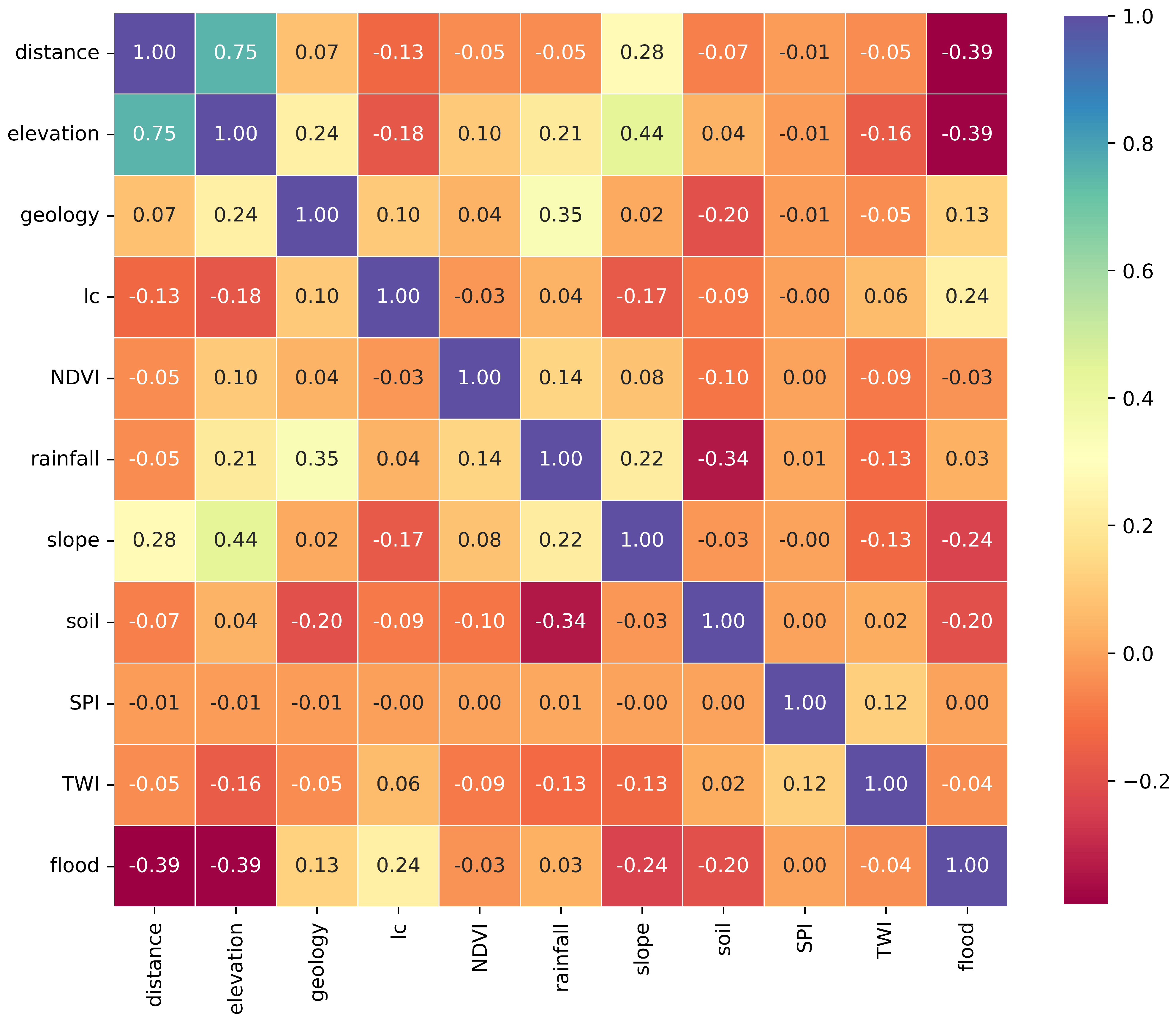
2.3. Flood Zones and Correlations
2.4. Machine Learning
2.4.1. Support Vector Machine
2.4.2. Artificial Neural Network
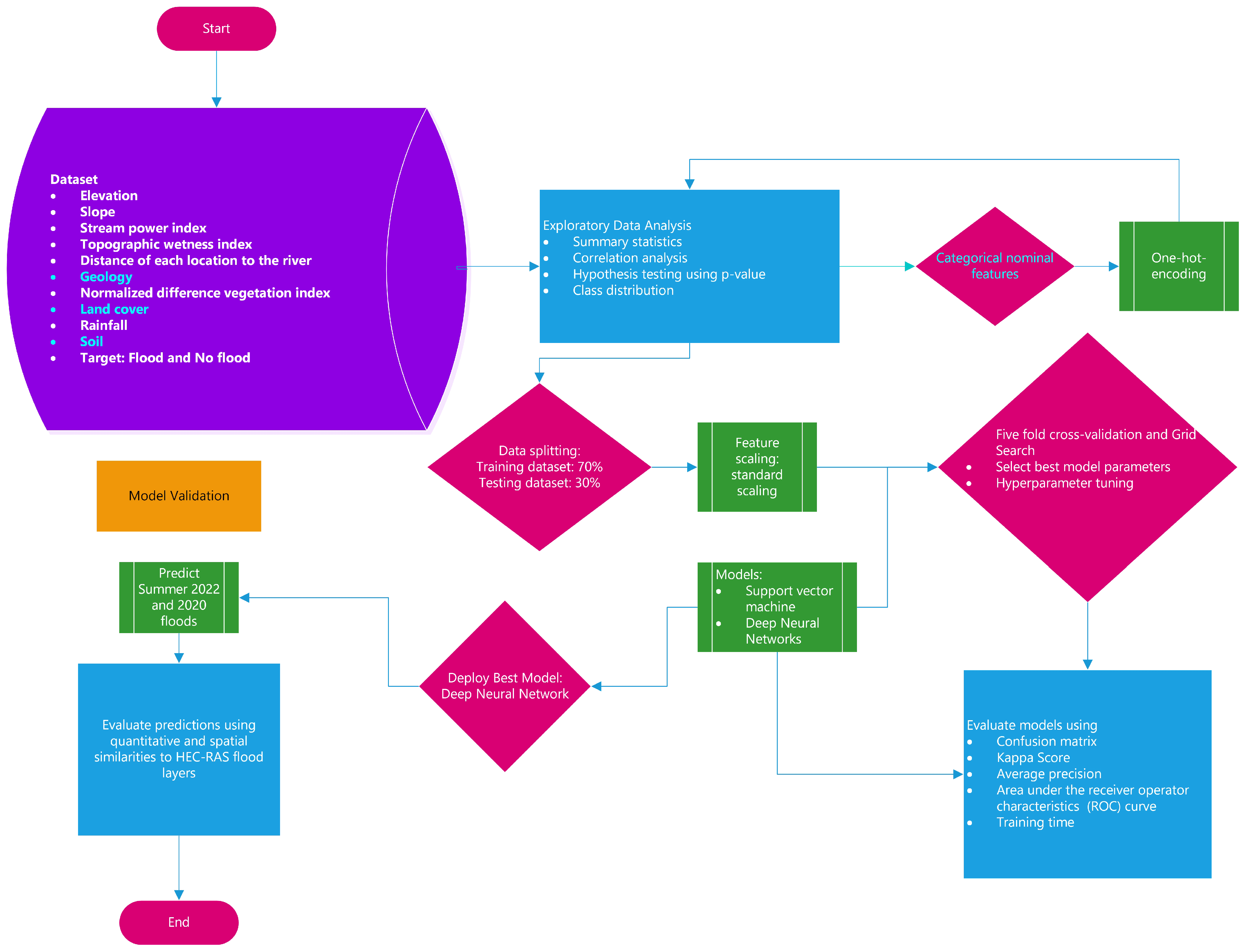
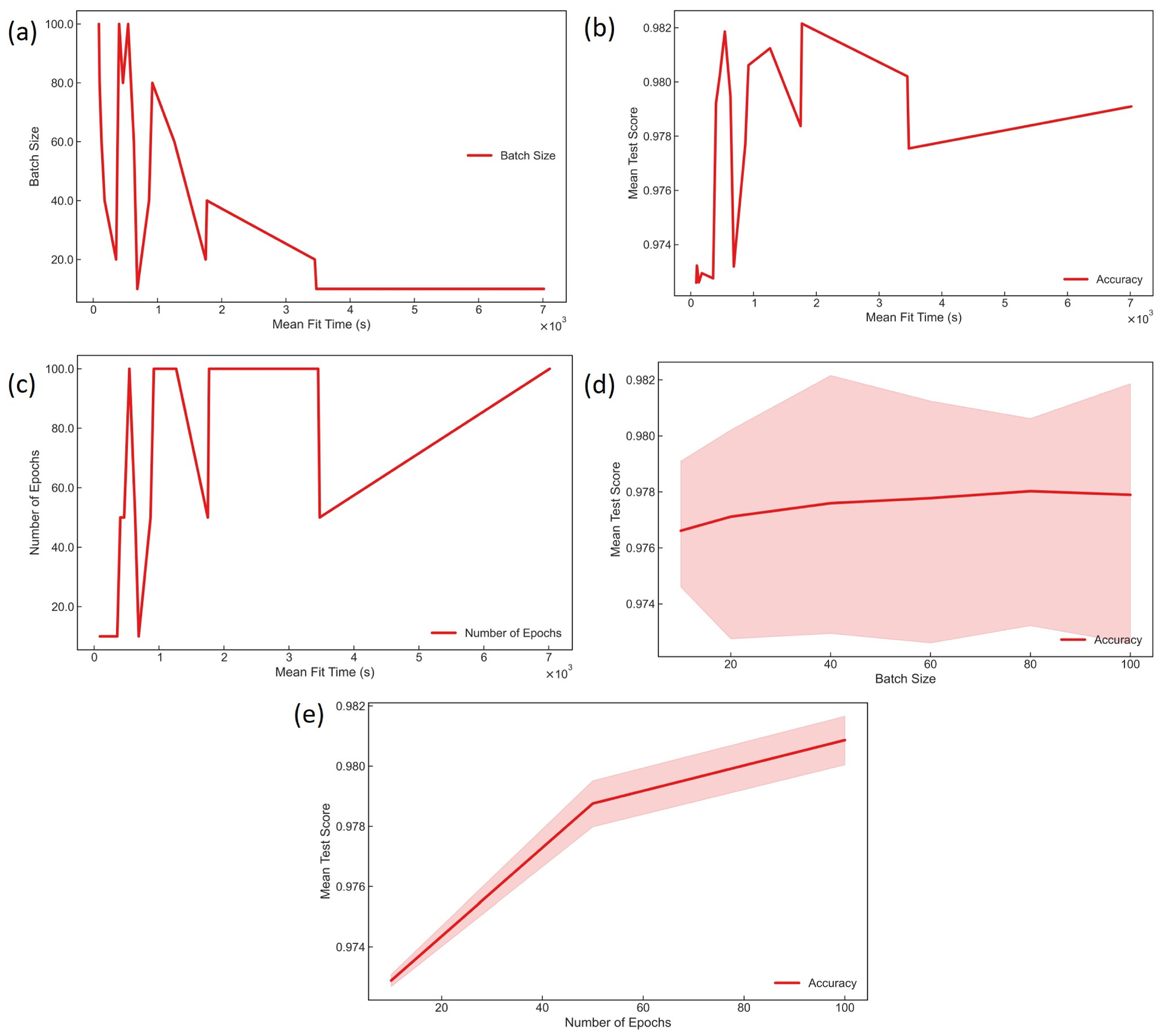
2.5. Machine-Learning Life Cycle
2.6. Cross-Validation
2.7. Models Assessment
3. Results
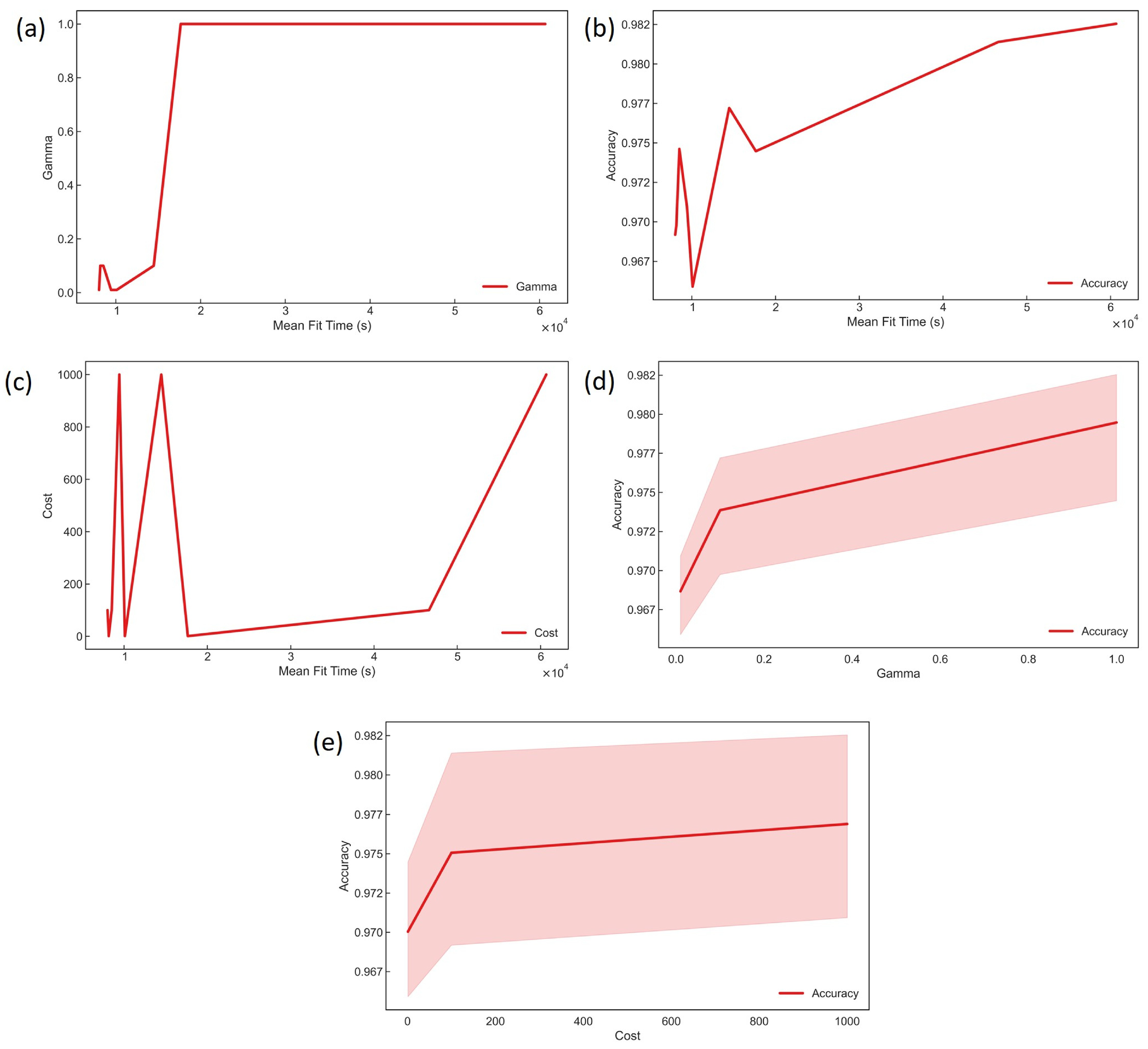
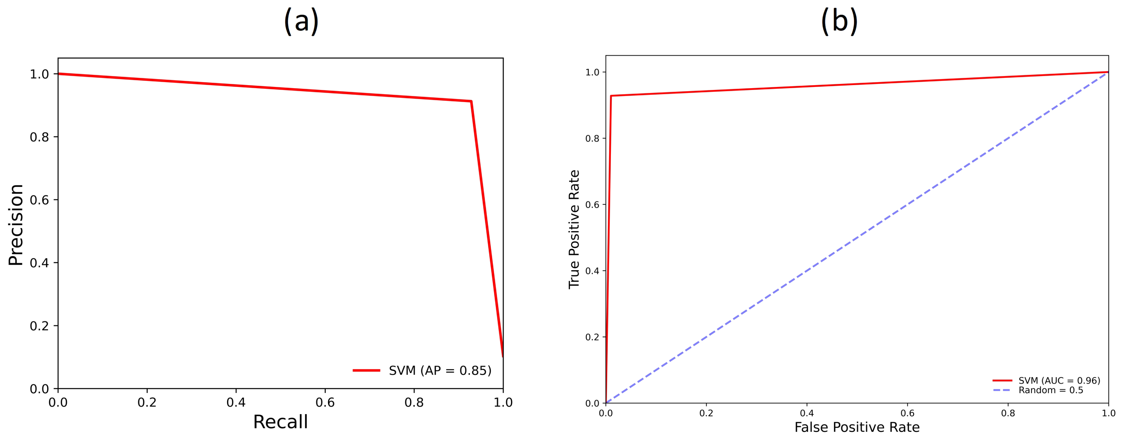
3.1. Support Vector Machine Models
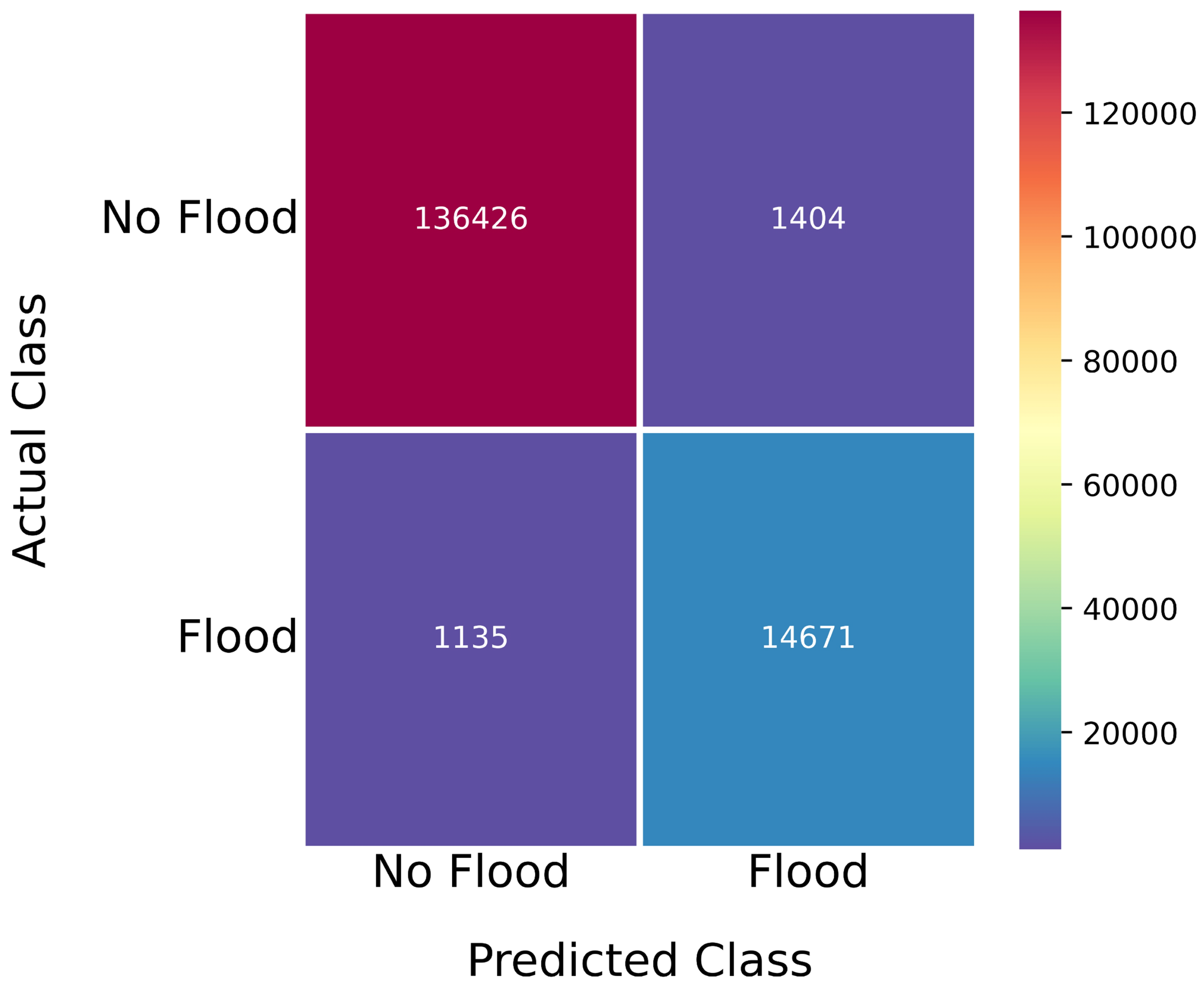
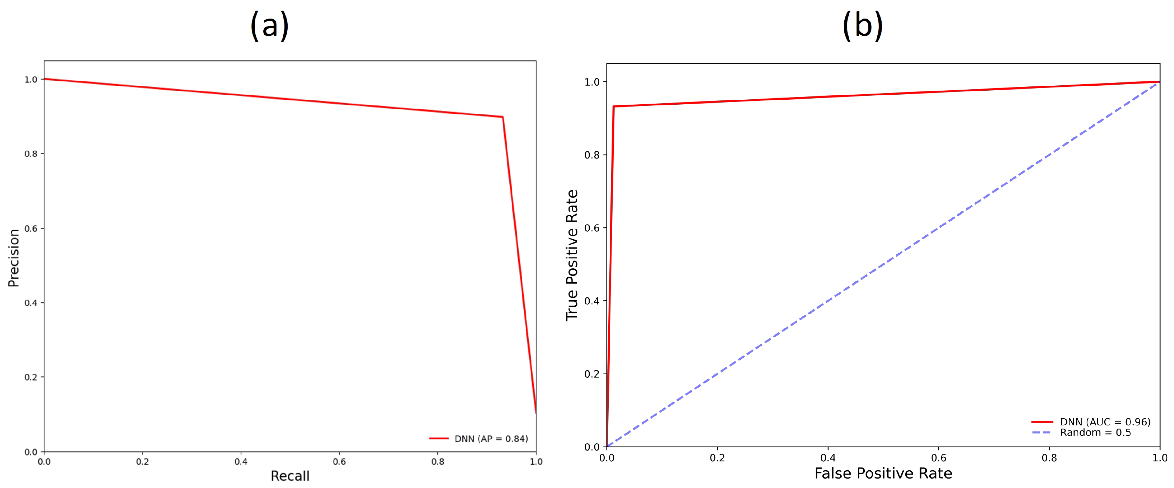
3.2. Deep Neural Network Models
4. Discussion
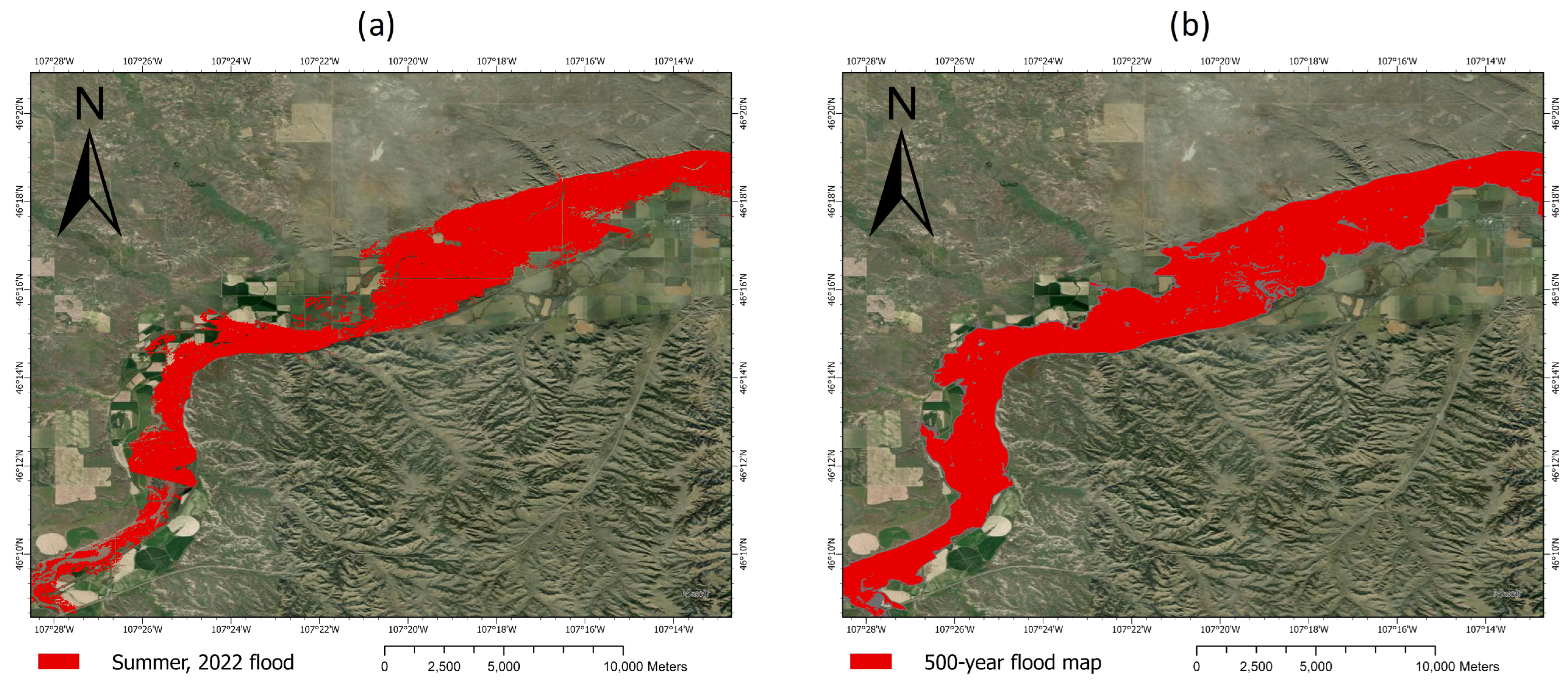
4.1. Model Validation
4.2. Statistical Methods
5. Conclusions
Author Contributions
Funding
Data Availability Statement
Acknowledgments
Conflicts of Interest
References
- Bell, L.; Bell, F.G. Geological Hazards: Their Assessment, Avoidance and Mitigation; CRC Press LLC: London, UK, 1999. [Google Scholar]
- USACE. Yellowstone River Corridor Study Hydraulic Analysis Modeling and Mapping Report; US Army Corps of Engineers, Omaha District: Omaha, NE, USA, 2016; p. 34.
- Fortin, J.P.; Turcotte, R.; Massicotte, S.; Moussa, R.; Fitzback, J.; Villeneuve, J.P. Distributed watershed model compatible with remote sensing and GIS data. I: Description of model. J. Hydrol. Eng. 2001, 6, 91–99. [Google Scholar] [CrossRef]
- Jayakrishnan, R.; Srinivasan, R.; Santhi, C.; Arnold, J.G. Advances in the application of the SWAT model for water resources management. Hydrol. Process. 2005, 19, 749–762. [Google Scholar] [CrossRef]
- Tehrany, M.S.; Pradhan, B.; Jebur, M.N. Spatial prediction of flood susceptible areas using rule based decision tree (DT) and a novel ensemble bivariate and multivariate statistical models in GIS. J. Hydrol. 2013, 504, 69–79. [Google Scholar] [CrossRef]
- Tien Bui, D.; Pradhan, B.; Nampak, H.; Bui, Q.T.; Tran, Q.A.; Nguyen, Q.P. Hybrid artificial intelligence approach based on neural fuzzy inference model and metaheuristic optimization for flood susceptibilitgy modeling in a high-frequency tropical cyclone area using GIS. J. Hydrol. 2016, 540, 317–330. [Google Scholar] [CrossRef]
- Jodar-Abellan, A.; Valdes-Abellan, J.; Pla, C.; Gomariz-Castillo, F. Impact of land use changes on flash flood prediction using a sub-daily SWAT model in five Mediterranean ungauged watersheds (SE Spain). Sci. Total Environ. 2019, 657, 1578–1591. [Google Scholar] [CrossRef] [PubMed]
- Kastridis, A.; Stathis, D. Evaluation of hydrological and hydraulic models applied in typical Mediterranean Ungauged watersheds using post-flash-flood measurements. Hydrology 2020, 7, 12. [Google Scholar] [CrossRef]
- Lee Myers, B. The Flood Disaster Protection Act of 1973. Am. Bus. Law J. 1976, 13, 315–334. [Google Scholar] [CrossRef]
- Kazakis, N.; Kougias, I.; Patsialis, T. Assessment of flood hazard areas at a regional scale using an index-based approach and Analytical Hierarchy Process: Application in Rhodope–Evros region, Greece. Sci. Total Environ. 2015, 538, 555–563. [Google Scholar] [CrossRef]
- Lee, M.J.; Kang, J.E.; Jeon, S. Application of frequency ratio model and validation for predictive flooded area susceptibility mapping using GIS. In Proceedings of the 2012 IEEE International Geoscience and Remote Sensing Symposium, Munich, Germany, 22–27 July 2012; pp. 895–898. [Google Scholar] [CrossRef]
- Benediktsson, J.A.; Swain, P.H.; Ersoy, O.K. Neural Network Approaches Versus Statistical Methods in Classification of Multisource Remote Sensing Data. IEEE Trans. Geosci. Remote Sens. 1990, 28, 540–552. [Google Scholar] [CrossRef]
- Tehrany, M.S.; Pradhan, B.; Jebur, M.N. Flood susceptibility analysis and its verification using a novel ensemble support vector machine and frequency ratio method. Stoch. Environ. Res. Risk Assess. 2015, 29, 1149–1165. [Google Scholar] [CrossRef]
- Tehrany, M.S.; Pradhan, B.; Mansor, S.; Ahmad, N. Flood susceptibility assessment using GIS-based support vector machine model with different kernel types. CATENA 2015, 125, 91–101. [Google Scholar] [CrossRef]
- Bui, D.T.; Pradhan, B.; Lofman, O.; Revhaug, I.; Dick, O.B. Application of support vector machines in landslide susceptibility assessment for the Hoa Binh province (Vietnam) with kernel functions analysis. In Proceedings of the iEMSs 2012-Managing Resources of a Limited Planet, 6th Biennial Meeting of the International Environmental Modelling and Software Society, Leipzig, Germany, 1–5 July 2012; pp. 382–389. [Google Scholar]
- Kia, M.B.; Pirasteh, S.; Pradhan, B.; Mahmud, A.R.; Sulaiman, W.N.A.; Moradi, A. An artificial neural network model for flood simulation using GIS: Johor River Basin, Malaysia. Environ. Earth Sci. 2012, 67, 251–264. [Google Scholar] [CrossRef]
- Konadu, D.; Fosu, C. Digital elevation models and GIS for watershed modelling and flood prediction–a case study of Accra Ghana. In Appropriate Technologies for Environmental Protection in the Developing World; Springer: Dordrecht, The Netherlands, 2009; pp. 325–332. [Google Scholar] [CrossRef]
- DeVries, B.; Huang, C.; Armston, J.; Huang, W.; Jones, J.W.; Lang, M.W. Rapid and robust monitoring of flood events using Sentinel-1 and Landsat data on the Google Earth Engine. Remote Sens. Environ. 2020, 240, 111664. [Google Scholar] [CrossRef]
- Vishnu, C.; Sajinkumar, K.; Oommen, T.; Coffman, R.; Thrivikramji, K.; Rani, V.; Keerthy, S. Satellite-based assessment of the August 2018 flood in parts of Kerala, India. Geomat. Nat. Hazards Risk 2019, 10, 758–767. [Google Scholar] [CrossRef]
- Patro, S.; Chatterjee, C.; Mohanty, S.; Singh, R.; Raghuwanshi, N.S. Flood inundation modeling using MIKE FLOOD and remote sensing data. J. Indian Soc. Remote Sens. 2009, 37, 107–118. [Google Scholar] [CrossRef]
- Ouaba, M.; Saidi, M.E.; Alam, M.J.B. Flood modeling through remote sensing datasets such as LPRM soil moisture and GPM-IMERG precipitation: A case study of ungauged basins across Morocco. Earth Sci. Inform. 2023, 16, 653–674. [Google Scholar] [CrossRef]
- El Alfy, M. Assessing the impact of arid area urbanization on flash floods using GIS, remote sensing, and HEC-HMS rainfall-runoff modeling. Hydrol. Res. 2016, 47, 1142–1160. [Google Scholar] [CrossRef]
- Khan, S.I.; Yang, H.; Wang, J.; Yilmaz, K.K.; Gourley, J.J.; Adler, R.F.; Brakenridge, G.R.; Policelli, F.; Habib, S.; Irwin, D. Satellite Remote Sensing and Hydrologic Modeling for Flood Inundation Mapping in Lake Victoria Basin: Implications for Hydrologic Prediction in Ungauged Basins. IEEE Trans. Geosci. Remote Sens. 2011, 49, 85–95. [Google Scholar] [CrossRef]
- Kourgialas, N.N.; Karatzas, G.P. Flood management and a GIS modelling method to assess flood-hazard areas—A case study. Hydrol. Sci. J. 2011, 56, 212–225. [Google Scholar] [CrossRef]
- Liu, Y.B.; Gebremeskel, S.; De Smedt, F.; Hoffmann, L.; Pfister, L. A diffusive transport approach for flow routing in GIS-based flood modeling. J. Hydrol. 2003, 283, 91–106. [Google Scholar] [CrossRef]
- Mason, L.A. GIS Modeling of Riparian Zones Utilizing Digital Elevation Models and Flood Height Data. Master’s Thesis, Michigan Technological University, Houghton, MI, USA, 2007. [Google Scholar]
- Schanze, J.; Zeman, E.; Marsalek, J. Flood Risk Management: Hazards, Vulnerability and Mitigation Measures, 1st. ed.; Nato Science Series: IV; Earth and Environmental Sciences, 67; Springer: Dordrecht, The Netherlands, 2006. [Google Scholar] [CrossRef]
- Tymkow, P.; Karpina, M.; Borkowski, A. 3D GIS for flood modelling in river valleys. Int. Arch. Photogramm. Remote Sens. Spat. Inf. Sci. 2016, XLI-B8, 175–178. [Google Scholar] [CrossRef]
- Ighile, E.H.; Shirakawa, H.; Tanikawa, H. Application of GIS and Machine Learning to Predict Flood Areas in Nigeria. Sustainability 2022, 14, 5039. [Google Scholar] [CrossRef]
- Motta, M.; de Castro Neto, M.; Sarmento, P. A mixed approach for urban flood prediction using Machine Learning and GIS. Int. J. Disaster Risk Reduct. 2021, 56, 102154. [Google Scholar] [CrossRef]
- Sresakoolchai, J.; Hamarat, M.; Kaewunruen, S. Automated machine learning recognition to diagnose flood resilience of railway switches and crossings. Sci. Rep. 2023, 13, 2106. [Google Scholar] [CrossRef] [PubMed]
- Elkhrachy, I. Flash Flood Water Depth Estimation Using SAR Images, Digital Elevation Models, and Machine Learning Algorithms. Remote Sens. 2022, 14, 440. [Google Scholar] [CrossRef]
- Zelt, R.B. Environmental Setting of the Yellowstone River Basin, Montana, North Dakota, and Wyoming; US Department of the Interior, US Geological Survey: Denver, CO, USA, 1999; Volume 98.
- Chase, K.J. Streamflow Statistics for Unregulated and Regulated Conditions for Selected Locations on the Yellowstone, Tongue, and Powder Rivers, Montana, 1928–2002; US Geological Survey: Reston, VA, USA, 2014.
- Papangelakis, E.; MacVicar, B.; Ashmore, P.; Gingerich, D.; Bright, C. Testing a Watershed-Scale Stream Power Index Tool for Erosion Risk Assessment in an Urban River. J. Sustain. Water Built Environ. 2022, 8, 04022008. [Google Scholar] [CrossRef]
- Micu, D.; Urdea, P. Vulnerable areas, the stream power index and the soil characteristics on the southern slope of the lipovei hills. Carpathian J. Earth Environ. Sci. 2022, 17, 207–218. [Google Scholar] [CrossRef]
- Cobin, P.F. Probablistic Modeling of Rainfall Induced landslide Hazard Assessment in San Juan La Laguna, Sololá, Guatemala. Master’s Thesis, Michigan Technological University, Houghton, MI, USA, 2013. [Google Scholar]
- Hong, H.; Chen, W.; Xu, C.; Youssef, A.M.; Pradhan, B.; Tien Bui, D. Rainfall-induced landslide susceptibility assessment at the Chongren area (China) using frequency ratio, certainty factor, and index of entropy. Geocarto Int. 2017, 32, 139–154. [Google Scholar] [CrossRef]
- Sorensen, R.; Zinko, U.; Seibert, J. On the calculation of the topographic wetness index: Evaluation of different methods based on field observations. Hydrol. Earth Syst. Sci. 2006, 10, 101–112. [Google Scholar] [CrossRef]
- Andrews, D.A.; Lambert, G.S.; Stose, G.W. Geologic Map of Montana; Report 25; U.S. Geological Survey: Denver, CO, USA, 1944. [CrossRef]
- Jain, V.; Sinha, R. Geomorphological Manifestations of the Flood Hazard: A Remote Sensing Based Approach. Geocarto Int. 2003, 18, 51–60. [Google Scholar] [CrossRef]
- Pettorelli, N.; Ryan, S.; Mueller, T.; Bunnefeld, N.; Jędrzejewska, B.; Lima, M.; Kausrud, K. The Normalized Difference Vegetation Index (NDVI): Unforeseen successes in animal ecology. Clim. Res. 2011, 46, 15–27. [Google Scholar] [CrossRef]
- Chander, G.; Markham, B.L.; Helder, D.L. Summary of current radiometric calibration coefficients for Landsat MSS, TM, ETM+, and EO-1 ALI sensors. Remote Sens. Environ. 2009, 113, 893–903. [Google Scholar] [CrossRef]
- Huffman, G.; Stocker, E.; Bolvin, D.; Nelkin, E.; Tan, J. GPM IMERG Late Precipitaion L3 1 Day 0.1 Degree x 0.1 Degree V06; Goddard Earth Sciences Data and Information Services Center (GES DISC): Greenbelt, MD, USA, 2019.
- UN-SPIDER. In Detail: Recommended Practice: Flood Mapping and Damage Assessment Using Sentinel-1 SAR Data in Google Earth Engine. Available online: https://un-spider.org/advisory-support/recommended-practices/recommended-practice-google-earth-engine-flood-mapping/in-detail (accessed on 13 October 2022).
- Kuhn, M.; Johnson, K. Applied Predictive Modeling, 1st ed.; Springer: New York, NY, USA, 2013. [Google Scholar] [CrossRef]
- Zhou, Z.H. Machine Learning; Springer: Gateway East, Singapore, 2021. [Google Scholar]
- Vapnik, V.N. Statistical Learning Theory; Adaptive and Learning Systems for Signal Processing, Communications, and Control; Wiley: New York, NY, USA, 1998. [Google Scholar]
- James, G. An Introduction to Statistical Learning: With Applications in R, 2nd ed.; Springer Texts in Statistics; Springer: New York, NY, USA, 2021. [Google Scholar]
- Lam, H.K.; Nguyen, H.T.; Ling, S.S.H. Computational Intelligence and Its Applications Evolutionary Computation, Fuzzy Logic, Neural Network and Support Vector Machine Techniques; Imperial College Press: London, UK, 2012. [Google Scholar]
- Haykin, S.S. Neural Networks: A Comprehensive Foundation, 2nd ed.; Prentice Hall: Upper Saddle River, NJ, USA, 1999. [Google Scholar]
- Werbos, P. Beyond Regression: New Tools for Prediction and Analysis in the Behavioral Sciences. Ph.D. Thesis, Committee on Applied Mathematics, Harvard University, Cambridge, MA, USA, 1974. [Google Scholar]
- Werbos, P.J. The Roots of Backpropagation: From Ordered Derivatives to Neural Networks and Political Forecasting; John Wiley & Sons: New York, NY, USA, 1994; Volume 1. [Google Scholar]
- Engelbrecht, A.P. Computational Intelligence: An Introduction, 2nd ed.; John Wiley & Sons Ltd.: Hoboken, NJ, USA, 2007. [Google Scholar] [CrossRef]
- Keller, J.M.; Liu, D.; Fogel, D.B. Fundamentals of Computational Intelligence: Neural Networks, Fuzzy Systems, and Evolutionary Computation, 1st ed.; IEEE Press Series on Computational Intelligence; Wiley: Newark, NY, USA, 2016. [Google Scholar] [CrossRef]
- Bhamare, D.; Suryawanshi, P. Review on reliable pattern recognition with machine learning techniques. Fuzzy Inf. Eng. 2018, 10, 362–377. [Google Scholar] [CrossRef]
- Liu, X.; Deng, Z.; Yang, Y. Recent progress in semantic image segmentation. Artif. Intell. Rev. 2019, 52, 1089–1106. [Google Scholar] [CrossRef]
- Jiang, H.; Peng, M.; Zhong, Y.; Xie, H.; Hao, Z.; Lin, J.; Ma, X.; Hu, X. A survey on deep learning-based change detection from high-resolution remote sensing images. Remote Sens. 2022, 14, 1552. [Google Scholar] [CrossRef]
- Qiu, M.; Qiu, H. Review on image processing based adversarial example defenses in computer vision. In Proceedings of the 2020 IEEE 6th Intl Conference on Big Data Security on Cloud (BigDataSecurity), IEEE Intl Conference on High Performance and Smart Computing, (HPSC) and IEEE Intl Conference on Intelligent Data and Security (IDS), Baltimore, MD, USA, 25–27 May 2020; IEEE: Piscatway, NJ, USA, 2020; pp. 94–99. [Google Scholar]
- Pierson, H.A.; Gashler, M.S. Deep learning in robotics: A review of recent research. Adv. Robot. 2017, 31, 821–835. [Google Scholar] [CrossRef]
- Wang, D.; Wang, X.; Lv, S. An overview of end-to-end automatic speech recognition. Symmetry 2019, 11, 1018. [Google Scholar] [CrossRef]
- Göçeri, E. Impact of deep learning and smartphone technologies in dermatology: Automated diagnosis. In Proceedings of the 2020 Tenth International Conference on Image Processing Theory, Tools and Applications (IPTA), Paris, France, 9–12 November 2020; IEEE: Piscatway, NJ, USA, 2020; pp. 1–6. [Google Scholar]
- Oommen, T.; Baise, L.G.; Vogel, R. Validation and application of empirical liquefaction models. J. Geotech. Geoenviron. Eng. 2010, 136, 1618–1633. [Google Scholar] [CrossRef]
- Rajaneesh, A.; Vishnu, C.; Oommen, T.; Rajesh, V.; Sajinkumar, K. Machine learning as a tool to classify extra-terrestrial landslides: A dossier from Valles Marineris, Mars. Icarus 2022, 376, 114886. [Google Scholar] [CrossRef]
- Krzanowski, W.J.; Hand, D.J. ROC Curves for Continuous Data, 1st ed.; Monographs on Statistics and Applied Probability; 111; Chapman & Hall/CRC: Boca Raton, FL, USA, 2009. [Google Scholar] [CrossRef]
- Cohen, J. A Coefficient of Agreement for Nominal Scales. Educ. Psychol. Meas. 1960, 20, 37–46. [Google Scholar] [CrossRef]
- Ozenne, B.; Subtil, F.; Maucort-Boulch, D. The precision–recall curve overcame the optimism of the receiver operating characteristic curve in rare diseases. J. Clin. Epidemiol. 2015, 68, 855–859. [Google Scholar] [CrossRef] [PubMed]
- Pedregosa, F.; Varoquaux, G.; Gramfort, A.; Michel, V.; Thirion, B.; Grisel, O.; Blondel, M.; Prettenhofer, P.; Weiss, R.; Dubourg, V.; et al. Scikit-learn: Machine Learning in Python. J. Mach. Learn. Res. 2011, 12, 2825–2830. [Google Scholar]
- Boyd, K.; Eng, K.H.; Page, C.D. Area under the Precision-Recall Curve: Point Estimates and Confidence Intervals; Springer, Machine Learning and Knowledge Discovery in Databases: Berlin/Heidelberg, Germany, 2013; pp. 451–466. [Google Scholar]
- Bamber, D. The area above the ordinal dominance graph and the area below the receiver operating characteristic graph. J. Math. Psychol. 1975, 12, 387–415. [Google Scholar] [CrossRef]
- Schütze, H.; Manning, C.D.; Raghavan, P. Introduction to Information Retrieval; Cambridge University Press Cambridge: Cambridge, UK, 2008; Volume 39. [Google Scholar]
- Tharwat, A. Classification assessment methods. Appl. Comput. Inform. 2021, 17, 168–192. [Google Scholar] [CrossRef]
- Berrar, D. On the noise resilience of ranking measures. In Proceedings of the Neural Information Processing: 23rd International Conference, ICONIP 2016, Kyoto, Japan, 16–21 October 2016; Proceedings, Part II 23; Springer: Berlin/Heidelberg, Germany, 2016; pp. 47–55. [Google Scholar]
- Hartman, J.; Kopič, D. Scaling TensorFlow to 300 million predictions per second. In Proceedings of the 15th ACM Conference on Recommender Systems, Amsterdam, The Netherlands, 27 September–1 October 2021; pp. 595–597. [Google Scholar]
- Dokuz, Y.; Tufekci, Z. Mini-batch sample selection strategies for deep learning based speech recognition. Appl. Acoust. 2021, 171, 107573. [Google Scholar] [CrossRef]
- Denis, R. Artificial Intelligence by Example: Acquire Advanced AI, Machine Learning, and Deep Learning Design Skills, 2nd ed.; Packt Publishing: Birmingham, UK, 2020. [Google Scholar]
- Hu, J.; Feng, X.; Zheng, Y. Number of Epochs of Each Model and Hyperband’s Classification Performance. In Proceedings of the 2021 2nd International Seminar on Artificial Intelligence, Networking and Information Technology (AINIT), Shanghai, China, 15–17 October 2021; IEEE: Piscatway, NJ, USA, 2021; pp. 500–503. [Google Scholar]
- Huffman, G.; Stocker, E.; Bolvin, D.; Nelkin, E.; Tan, J. GPM IMERG Early Precipitation L3 1 Day 0.1 Degree x 0.1 Degree V06; Goddard Earth Sciences Data and Information Services Center (GES DISC): Greenbelt, MD, USA, 2019.
- Kreyszig, E.; Kreyszig, H.; Norminton, E.J. Advanced Engineering Mathematics, 10th ed.; Wiley: Hoboken, NJ, USA, 2011. [Google Scholar]
- Beatty, W. Decision Support Using Nonparametric Statistics, 1st ed.; SpringerBriefs in Statistics; Springer International Publishing: Cham, Switzerland, 2018. [Google Scholar] [CrossRef]
- Kokoska, S.; Zwillinger, D. CRC Standard Probability and Statistics Tables and Formulae; CRC Press: Boca Raton, FL, USA, 2000. [Google Scholar]
- Conover, W.J. Practical Nonparametric Statistics; John Wiley & Sons: New York, NY, USA, 1971; pp. 97–104. [Google Scholar]


| Dataset | Source | Data Type | Resolution (m) |
|---|---|---|---|
| Elevation | USGS | Raster | 30 |
| Geology | USGS | Vector | Variable |
| Normalized Difference Vegetation Index | Computed using GEE with Landsat 8 image | Raster | 30 |
| Normalized Difference Water Index | Computed using ArcGIS Pro using Landsat 8 image | Raster | 30 |
| Slope | Computed using ArcGIS Pro using digital elevation model | Raster | 30 |
| Stream power index | Computed using ArcGIS Pro using digital elevation model | Raster | 30 |
| Topographic wetness index | Computed using ArcGIS Pro using digital elevation model | Raster | 30 |
| Land cover | Multi-Resolution Land Characteristics Consortium | Raster | 30 |
| Flood zones | HEC-RAS and GEE flood analysis | Vector | 30 |
| Rainfall | Multi-satellite precipitation data downloaded from Earthdata NASA | HDF5 | 10,000 |
| Flood Dates | |||||
|---|---|---|---|---|---|
| 3/16/2003 | 5/23/2011 | 7/2/2011 | 3/10/2014 | 6/7/2017 | 6/8/2017 |
| 3/23/2018 | 5/28/2018 | 5/29/2018 | 5/30/2018 | 6/8/2019 | 6/9/2019 |
| 6/10/2019 | 6/2/2020 | 6/3/2020 | 6/4/2020 | 6/15/2022 | |
| Before Flood SAR Image | After Flood Image SAR Image | Difference Threshold | ||
|---|---|---|---|---|
| Start Date | End Date | Start Date | End Date | |
| 06/02/2017 | 06/06/2017 | 06/07/2017 | 06/09/2017 | 1.15 |
| 05/24/2018 | 05/26/2018 | 05/29/2018 | 06/01/0218 | 1.00 |
| 06/05/2019 | 06/07/2019 | 06/08/2019 | 06/11/2019 | 1.05 |
| Test Statistic | |||||
|---|---|---|---|---|---|
| Validation Map Pair | Results | Mann–Whitney U Test | Spearman’s Rank | Wilcoxon Signed-Rank Test | Conclusion |
| Summer 2022 flood & 500-year flood maps | p-value | 0 | 0 | 0 | Reject |
| statistics | 0.8 | ||||
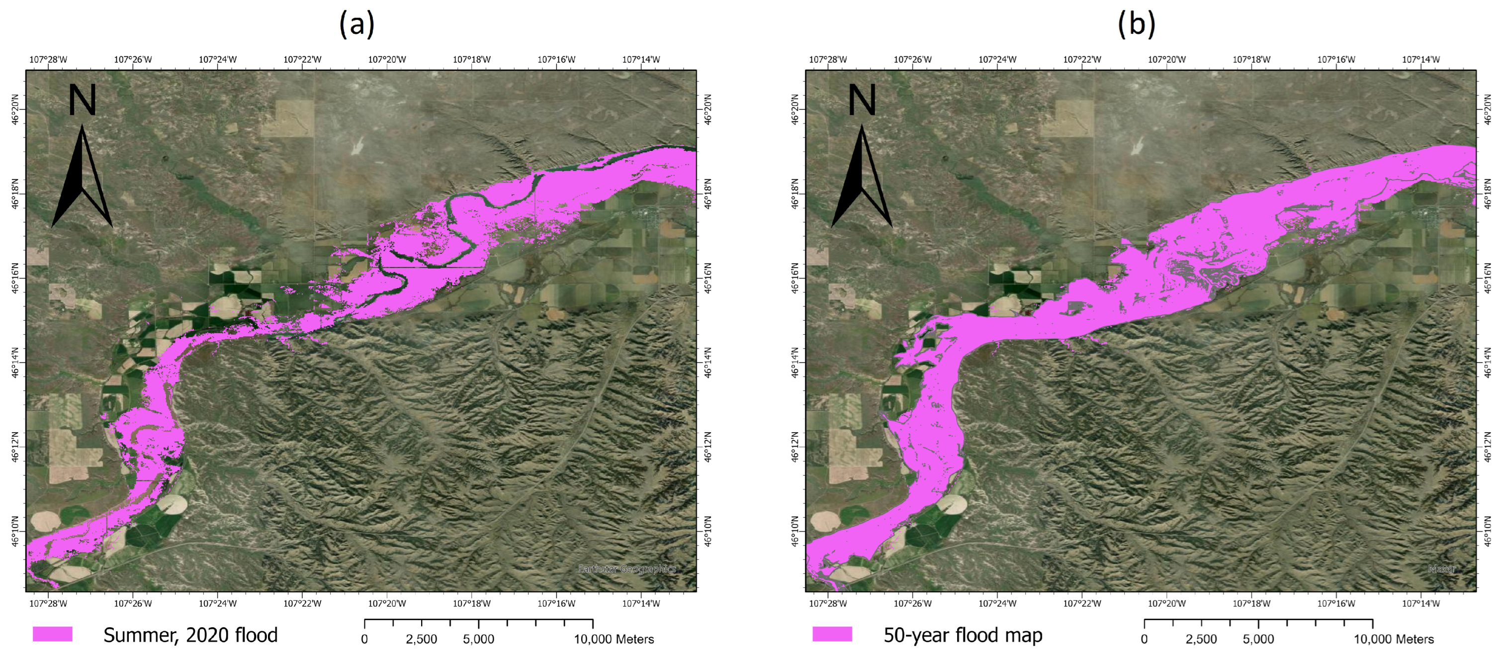
| Summer 2020 flood & 50-year flood maps | p-value | 0 | 0 | 0 | Reject |
| statistics | 0.69 | ||||
Disclaimer/Publisher’s Note: The statements, opinions and data contained in all publications are solely those of the individual author(s) and contributor(s) and not of MDPI and/or the editor(s). MDPI and/or the editor(s) disclaim responsibility for any injury to people or property resulting from any ideas, methods, instructions or products referred to in the content. |
© 2024 by the authors. Licensee MDPI, Basel, Switzerland. This article is an open access article distributed under the terms and conditions of the Creative Commons Attribution (CC BY) license (https://creativecommons.org/licenses/by/4.0/).
Share and Cite
Zakaria, A.-R.; Oommen, T.; Lautala, P. Automated Flood Prediction along Railway Tracks Using Remotely Sensed Data and Traditional Flood Models. Remote Sens. 2024, 16, 2332. https://doi.org/10.3390/rs16132332
Zakaria A-R, Oommen T, Lautala P. Automated Flood Prediction along Railway Tracks Using Remotely Sensed Data and Traditional Flood Models. Remote Sensing. 2024; 16(13):2332. https://doi.org/10.3390/rs16132332
Chicago/Turabian StyleZakaria, Abdul-Rashid, Thomas Oommen, and Pasi Lautala. 2024. "Automated Flood Prediction along Railway Tracks Using Remotely Sensed Data and Traditional Flood Models" Remote Sensing 16, no. 13: 2332. https://doi.org/10.3390/rs16132332