Advancing Regional–Scale Spatio–Temporal Dynamics of FFCO₂ Emissions in Great Bay Area

Abstract

Estimating city–scale emissions using gridded inventories lacks direct, precise measurements, resulting in significant uncertainty. A Kalman filter integrates diverse, uncertain information sources to deliver a reliable, accurate estimate of the true system state. By leveraging multiple gridded inventories and a Kalman filter fusion method, we developed an optimal city–scale (3 km) FFCO₂ emission product that incorporates quantified uncertainties and connects global–regional–city scales. Our findings reveal the following: (1) Kalman fusion post–reconstruction reduces estimate uncertainties for 2000–2014 and 2015–2021 to ±9.77% and ±11.39%, respectively, outperforming other inventories and improving accuracy to 73% compared to ODIAC and EDGAR (57%, 65%). (2) Long–term trends in the Greater Bay Area (GBA) show an upward trajectory, with a 2.8% rise during the global financial crisis and a −0.19% decline during the COVID-19 pandemic. Spatial analysis uncovers a “core–subcore–periphery” emission pattern. (3) The core city GZ consistently contributes the largest emissions, followed by DG as the second–largest emitter, and HK as the seventh–highest emitter. Factors influencing the center–shift of the pattern include the urban form of cities, population migration, GDP contribution, but not electricity consumption. The reconstructed method and product offer a reliable solution for the lack of directly observed emissions, enhancing decision–making accuracy for policymakers.

1. Introduction

Urban areas, covering just 2% of the Earth’s surface, are responsible for over 70% of global CO₂ emissions [1]. In 2020, global fossil fuel CO₂ (FFCO₂) emissions surpassed 38 Gt, constituting more than 77% of total fossil fuel greenhouse gas (GHG) emissions worldwide [2]. Cities themselves contribute over 70% of global FFCO₂ emissions [3,4] making them crucial units for implementing mitigation policies [5]. The IPCC emphasizes the significant emission reduction potential in urban areas, which are both vulnerable to climate change impacts and pivotal for effective solutions [6]. Despite this potential, enacting mitigation measures at the city level remains challenging; each city’s unique natural environment, economic status, urbanization level, industrial composition, and energy consumption profoundly influence its carbon emissions. The diverse emissions and socio–economic profiles among cities necessitate tailored policy approaches. China, experiencing rapid economic growth and urbanization, generates 85% of its direct carbon emissions from cities, contributing over 27% to global CO₂ emissions [7,8]. Pressure mounts on China to implement effective urban strategies for emission reduction and economic growth alignment. Therefore, a precise quantification of urban FFCO₂ emissions is essential for crafting mitigation policies that support global warming goals, including achieving carbon neutrality by 2050 [9].

Three main methods are commonly used to estimate fossil fuel CO₂ (FFCO₂) emissions: bottom–up, top–down, and hybrid approaches [3,5,10]. Top–down methods rely on atmospheric and inversion modeling to independently estimate emissions, emphasizing a production–based accounting method. These methods are valuable for assessing energy flows between regions and countries, and for evaluating city–level bottom–up estimates [11,12]. While top–down methods have shifted focus from global/continental to regional scales, they have proven to be more efficient for non–CO₂ greenhouse gases [13]. Bottom–up methods estimate FFCO₂ emissions employing standardized protocols, multiplying sectoral activity data (e.g., fuel sales) with pre–calculated emission factors for various socio–economic sources at every stage of human activity and a life cycle analysis (LCA) [14,15]. However, at finer spatial scales, the proxy approach may not accurately capture emission source distributions [16]. The hybrid approach integrates bottom–up, top–down, and other methods, utilizing global gridded emission inventories to downscale total FFCO₂ emissions to finer resolutions over specific spatial and temporal intervals [3]. This downscaling involves using spatial surrogates, such as population density [17], land use [18], or nighttime lights [19,20], or combining point sources like power plants [21] and line sources like on–road emissions [22,23], to construct high–resolution urban FFCO₂ emission maps. Multi–source spatial proxies and linear and panel regression models aid in downscaling emissions and resolution enhancement. Uncertainty in emission estimates is categorized into magnitude uncertainty linked to pre–downscaled emissions, which are typically provided by national fuel consumption accounts [24], and disaggregation uncertainty, which is associated with the downscaling process, stemming from imperfect spatial proxies [25]. Uncertainties persist in bottom–up emission estimates at regional and city scales, largely due to data gaps, insufficient information on energy and fuel use statistics, and outdated or inaccurate emission factors [16], with city–scale uncertainties ranging from 50% to 250% for the northeast USA [26] and up to 300% for the Beijing–Tianjin–Hebei region [27]. These uncertainties surrounding bottom–up inventories hinder the development of urban carbon emissions mitigation strategies [28]. The current body of research predominantly centers on leveraging multi–source spatial proxies to facilitate downscaled emissions and resolution enhancement with the aim of mitigating uncertainty. Alternatively, various bottom–up FFCO₂ emission inventories are juxtaposed to ascertain discrepancies between them. However, there remains a scarcity of fusion or reconstruction methodologies that amalgamate the strengths of diverse emission datasets to ascertain the optimal regional spatial resolution of fossil fuel CO₂ emissions.

In light of the aforementioned efforts, this paper aims to enhance the understanding of the uncertainty and spatial–temporal dynamics of FFCO₂ emission in the Guangdong–Hong Kong–Macao Greater Bay Area (GBA) through a comparative analysis of three hig–precision global FFCO₂ emission products and a fusion algorithm based on a Kalman filter at an urban scale. This paper addresses the question of the optimal spatial resolution for the fusion of FFCO₂ emission products, with the objective of reconstructing a set of FFCO₂ emission data products representative of regional scale characteristics at 3 km in the GBA. Through rigorous verification, our dataset, combined with auxiliary data sources such as nighttime light (NTL), Gross Domestic Product (GDP), population density (POP), and land use (LU), was utilized to examine the contributing factors influencing FFCO₂ emissions in both urban and rural areas.

2. Materials and Methods

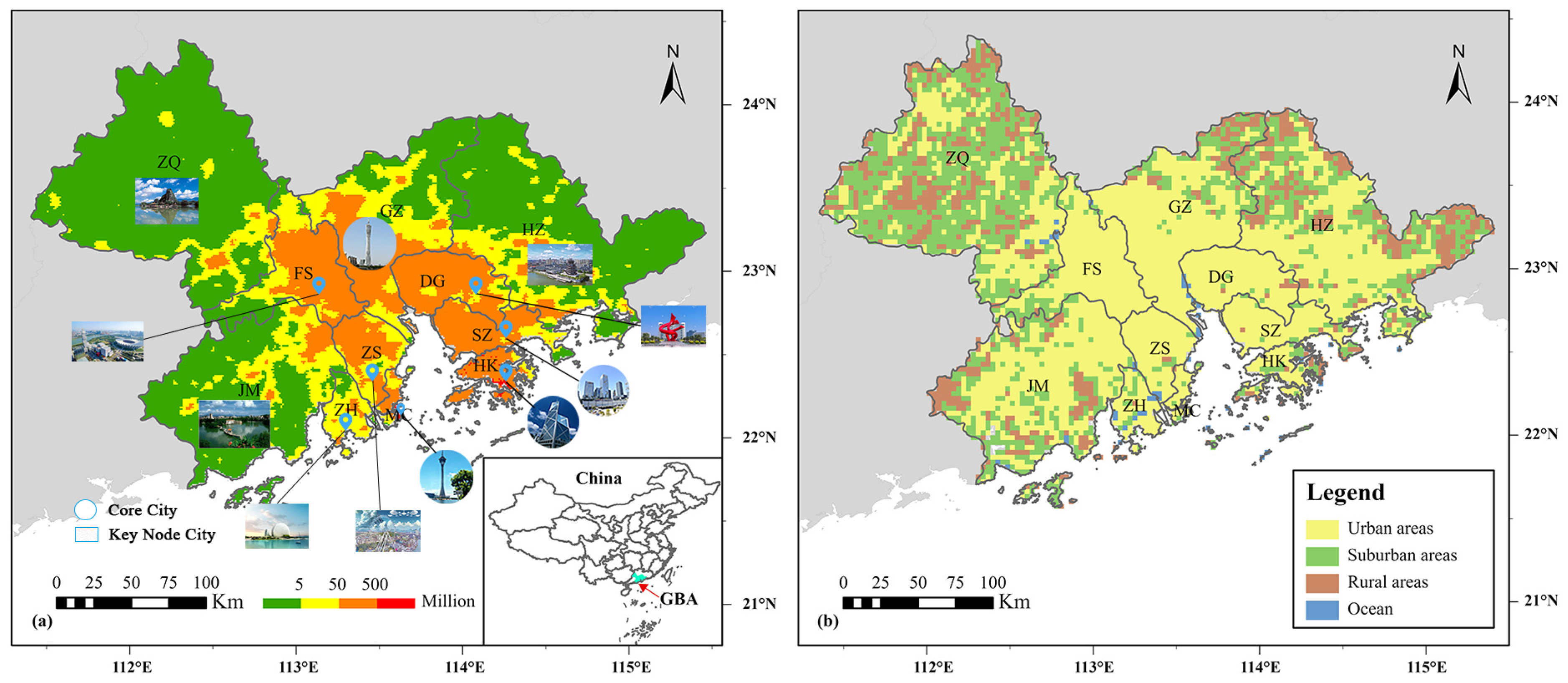
2.1. Study Area

The GBA is a prominent city cluster located in southern China, comprising 11 cities within Guangdong province (see Figure 1a). With a total area of 56,000 km² and a population of approximately 86.69 million as of the end of 2021, the region boasts a complete industrial system, a high concentration of innovative elements, and a high degree of internationalization. Recognized as one of China’s most open and economically dynamic regions [29], the GBA has achieved a level of development comparable to that of established economies [30]. The Guangdong–Hong Kong–Macau Bay Area Development Plan Outline [31], unveiled in 2019, underscores the importance of leveraging the combined advantages of Guangdong (GD), Hong Kong (HK), and Macao (MC) to drive deeper integration within the region, foster coordinated economic development, and construct an international world–class bay area suitable for living, working and traveling. Additionally, the GBA is committed to promoting ecological conservation, embracing green development goals, and advancing sustainable practices. The GBA’s new mission centers on pursuing green, low–carbon circular development and establishing itself as a model of green development excellence.

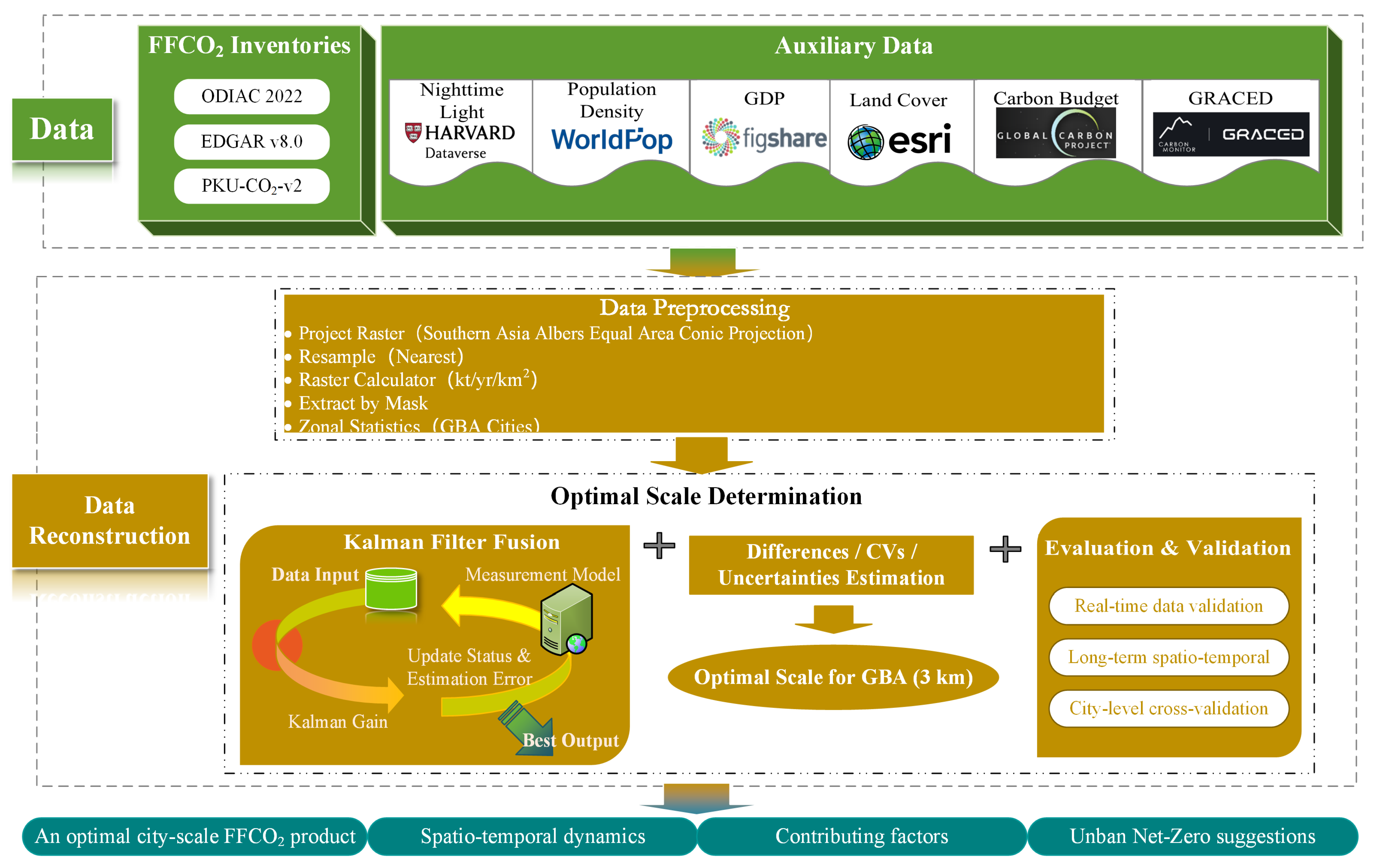
2.2. Gridded High–Resolution FFCO₂ Emission Inventories and Auxiliary Socio–economic Data

Gridded high–resolution emission inventories, commonly used to pinpoint emission hotspots, rely on emission bookkeeping and subsequent spatial and temporal allocation to create a gridded emission dataset, typically at a spatial resolution of 1–10 km [32]. The spatial allocation of high–resolution grid emission data often involves the use of proxy variables as allocation factors to distribute total emissions at a finer scale through a downscaling technique. However, this method inherently introduces uncertainty, particularly as the correlation between the proxy variable and emissions diminishes. In this study, three inventories served as the primary data sources for data reconstruction, with one near–real–time dataset employed for verification purposes (Table 1).

The Emissions Database for Global Atmospheric Research (EDGARv7.0) undergoes evaluation by the Joint Research Center (JRC) of the European Commission and the Netherlands Environmental Assessment Agency using Bayesian Estimation and Optimization (BEO) methodology. International Energy Agency (IEA) CO₂ emissions from fossil fuel combustion sources have been included to harmonize global CO₂ emission estimates. Notably, EDGARv7.0 features updated activity data types, including combustion–related and agriculture–related emissions, along with refined spatial proxies for electricity generation, industrial facilities, intensive livestock, population distribution, and non–residential areas [33,34]. This cutting–edge inventory dataset offers consistent harmonized global monthly FFCO₂ emissions in 16 sectors on a 0.1° × 0.1° resolution grid, covering an extensive time series from 1970 to 2021 [35]. The Open–Source Data Inventory for Anthropogenic CO₂ (ODIAC2022), commonly integrated into flux inversions and urban carbon emission estimates [4,36,37], was developed by the National Institute for Environmental Studies (NIES). ODIAC2022 downscales national FFCO₂ emission estimates from the Carbon Dioxide Information Analysis Center (CDIAC) by incorporating various spatial proxies, such as individual power plant emissions, location profiles, nightlight observations, and aircraft and ship fleet tracks for FFCO₂ distribution. Evolving since its initial release in 2011, ODIAC2022 has been enhanced through collaborations with the National Aeronautics and Space Administration (NASA) Black Marble Nighttime light product suite (VNP46) (available at 500 m resolution) [38] and the latest country–level FFCO₂ estimates (2000–2019) from the CDIAC team at the Appalachian State University [39]. The most recent iteration, ODIAC2022, spans from 2000 to 2021and is available in two resolutions/formats: 1 km × 1 km/GeoTIFF and 1° × 1°/NetCDF. The Peking University CO₂ emission inventory version 2 (PKU–CO₂–v2) [40] was developed using a bottom–up subnational disaggregation method (SDM) [21] based on 64 fuel subtypes across 5 categories and 6 sectors, featuring a spatial resolution of 0.1° × 0.1° and a monthly temporal resolution spanning from 1960 to 2014. A collaborative effort between Peking University, the French Laboratory of Climate and Environmental Sciences, and the Sino–French Institute for Earth System Science, this product provides detailed insights into CO₂ emissions at a subnational level.

The near–real–time Global Gridded Daily CO₂ Emissions Dataset (GRACED) developed by Tsinghua University offers a detailed gridded representation of CO₂ emissions at a spatial resolution of 0.1° × 0.1° and a temporal resolution of 1 day, focusing on emissions from cement production and fossil fuel combustion in seven sectors [41]. GRACED integrates near–real–time daily national CO₂ emission estimates from Carbon Monitoring [42], spatial activity data emissions from multiple sources, and satellite NO₂ data to capture temporal variations in these spatial activities. Notably, GRACED introduces a grid–level two–sigma uncertainty of ±19.9% in 2021 [43], underscoring the dataset’s reliability, despite its enhanced spatio–temporal resolution. This meticulous approach ensures that the precision of GRACED remains robust, while providing detailed insights into daily CO₂ emissions dynamics.

Table 1. Information about the high–resolution grided FFCO₂ emission inventories used in this study.

	Datebase	EDGARv7.0	ODIAC2022	PKU–CO2–v2	GRACED
Property
Level		National–level data	National– and subnational–level data	National– and subnational–level data	Global and national
Methodology		Bottom–up, transparent, and IPCC–compliant approach	Downscaled with multiple spatial proxy data (geographical location of point sources, satellite observations of nightlights, and aircraft and ship fleet tracks, etc.)	Bottom–up apparent consumption	Hybrid methods
Time window		1970–2021	2000–2021	1960–2014	January 2019–October 2023
Spatial resolution		0.1° × 0.1°	1 km × 1 km/1° × 1°	0.1° × 0.1°	0.1° × 0.1°
Original unit		kg m−2 s−1	tonne carbon/cell	G km−2 month−1	kgC/h
Fossil CO2 sources		Fossil fuel combustion, metal (ferrous and non–ferrous) production processes, non–metallic mineral processes (such as cement production), urea production, agricultural liming, and solvent use	Fuel use (coal, oil, and gas), cement production, and gas flaring	Wildfires, natural gas flaring, agricultural solid wastes, non–organized waste incineration, dung cake, others	Power, industry, residential consumption, ground transportation, domestic aviation, international aviation, and international shipping
Point source		CARbon Monitoring and Action (CARMA: www.carma.org), the place of the industrial facilities	CARMA	CARMA	N/A
Non–point source		Agricultural fields, population, nighttime light	Nighttime light (VNP46)	Population, nighttime light, vegetation	Hourly datasets of electric power production and associated CO2 emissions in 31 countries
Aviation		Road network	U.N. statistical data (AERO2k)	Using CO emissions as a proxy	TomTom, Paris data, EDGAR “road transportation” sector, Flightradar24, EDGAR shipping emissions
Download link		EDGAR 7.0. Available online: https://edgar.jrc.ec.europa.eu/dataset_ghg70 (accessed on 28 June 2023)	ODIAC2022. Available online: http://db.cger.nies.go.jp/dataset/ODIAC/ (accessed on 28 June 2023)	PKU–Fuel. Available online: https://gems.sustech.edu.cn/ (Previous website is http://inventory.pku.edu.cn/, accessed on 28 June 2023)	GRACED. Available online: https://carbonmonitor-graced.com/index.html (accessed on 28 June 2023)
Reference		[44,45,46]	[16,19,47]	[21,48,49]	[41,42,43,50]

Table 1. Information about the high–resolution grided FFCO₂ emission inventories used in this study.

	Datebase	EDGARv7.0	ODIAC2022	PKU–CO2–v2	GRACED
Property
Level		National–level data	National– and subnational–level data	National– and subnational–level data	Global and national
Methodology		Bottom–up, transparent, and IPCC–compliant approach	Downscaled with multiple spatial proxy data (geographical location of point sources, satellite observations of nightlights, and aircraft and ship fleet tracks, etc.)	Bottom–up apparent consumption	Hybrid methods
Time window		1970–2021	2000–2021	1960–2014	January 2019–October 2023
Spatial resolution		0.1° × 0.1°	1 km × 1 km/1° × 1°	0.1° × 0.1°	0.1° × 0.1°
Original unit		kg m−2 s−1	tonne carbon/cell	G km−2 month−1	kgC/h
Fossil CO2 sources		Fossil fuel combustion, metal (ferrous and non–ferrous) production processes, non–metallic mineral processes (such as cement production), urea production, agricultural liming, and solvent use	Fuel use (coal, oil, and gas), cement production, and gas flaring	Wildfires, natural gas flaring, agricultural solid wastes, non–organized waste incineration, dung cake, others	Power, industry, residential consumption, ground transportation, domestic aviation, international aviation, and international shipping
Point source		CARbon Monitoring and Action (CARMA: www.carma.org), the place of the industrial facilities	CARMA	CARMA	N/A
Non–point source		Agricultural fields, population, nighttime light	Nighttime light (VNP46)	Population, nighttime light, vegetation	Hourly datasets of electric power production and associated CO2 emissions in 31 countries
Aviation		Road network	U.N. statistical data (AERO2k)	Using CO emissions as a proxy	TomTom, Paris data, EDGAR “road transportation” sector, Flightradar24, EDGAR shipping emissions
Download link		EDGAR 7.0. Available online: https://edgar.jrc.ec.europa.eu/dataset_ghg70 (accessed on 28 June 2023)	ODIAC2022. Available online: http://db.cger.nies.go.jp/dataset/ODIAC/ (accessed on 28 June 2023)	PKU–Fuel. Available online: https://gems.sustech.edu.cn/ (Previous website is http://inventory.pku.edu.cn/, accessed on 28 June 2023)	GRACED. Available online: https://carbonmonitor-graced.com/index.html (accessed on 28 June 2023)
Reference		[44,45,46]	[16,19,47]	[21,48,49]	[41,42,43,50]

Four key socio–economic indicators—NTL, GDP, POP, and LU—served as foundational data for our spatio–temporal dynamics analysis. We leveraged an extensive time series spanning 2000 to 2018 of NPP–VIIRS–like NTL data [51] in the WGS84 coordinate system, boasting a spatial resolution of approximately 500 m. This dataset, available on the Harvard Dataverse website (https://dataverse.harvard.edu/, accessed on 15 March 2024), is the product of a unique cross–sensor calibration approach that integrates a vegetation index and an auto–encoder model built on two types of stable NTL data. In addition, global 1 km × 1 km gridded revised real GDP data [52], covering the period from 1992 to 2019, are openly accessible on Figshare (https://figshare.com/, accessed on 15 March 2024). This dataset, derived from another continuous and calibrated NTL dataset, offers a growth rate perspective with a top–down method optimized using Particle Swarm Optimization–Back Propagation (PSO–BP). Furthermore, the WorldPop datasets provide detailed POP data for individual countries for the years 2000 to 2020 (https://hub.worldpop.org/project/categories?id=18/, accessed on 15 March 2024) with a resolution of approximately 1 km at the equator for all nations globally. These datasets are generated by dividing the population count in each pixel by the pixel surface area, using an unconstrained top–down methodology.

Sentinel–2 multispectral imagery has proven instrumental in land use/land cover (LULC) monitoring for urban area mapping [53] and carbon assessments [54]. We delineated the Urban–Rural Divide (see Figure 1b) of the GBA by utilizing a 10 m annual land use/land cover (9–class) dataset, derived from high–resolution Sentinel–2 imagery. The segmentation process employed cutting–edge deep learning AI techniques, made freely accessible through the Esri Sentinel–2 Land Cover Explorer (https://livingatlas.arcgis.com/landcoverexplorer/, accessed on 29 June 2023). The primary objective of this divide is to elucidate the impact of the complex interplay of socio–economic factors on transition dynamics and cross–border emission patterns. It is evident that internal urban and rural development levels among the city cluster are uneven, with suburban areas and rural areas dispersed throughout the 11 cities. Grids with a resolution of 3 km were established on the Esri Sentinel–2 Land Cover Type (LCT) within ArcGIS to align with the GBA scale. The categorization into “Urban areas”, “Rural areas”, “Suburban areas”, and “Ocean areas” was based on the proportions of “Built areas” or “Water areas” within each grid. The classification criteria [55] were defined as follows, and the 10 m–resolution land cover product enhanced the accuracy of the classification results: (1) grids with a “Built areas” proportion > 10% were classified as “Urban areas”; (2) grids with a “Built areas” proportion between 1% and 10% were classified as “Suburban areas”; (3) grids with a “Built areas” proportion < 1% were classified as “Rural areas”; and (4) grids with a “Water” proportion > 80% were classified as “Ocean areas”. This methodology provides a comprehensive framework for characterizing land use patterns within the GBA region.

2.3. Fine Spatial Resolution Fusion Method

Accurately characterizing spatial and temporal patterns of urban surface emissions poses a challenge for individual FFCO₂ emission inventories. The differences and coefficients of variation (CVs) among these inventories must be quantified and incorporated into the reconstruction algorithm. A crucial aspect of the reconstruction process is establishing a connection between global and regional scales. Various studies have demonstrated that leveraging mathematical models such as regression, assimilation, and neural networks, along with data sources like population figures, road networks, and NTL data, can significantly enhance the accuracy of the spatio–temporal allocation of FFCO₂ emission inventories [56]. This study introduces a Kalman filter fusion algorithm to reconstruct a new FFCO₂ emission dataset at regional and urban scales. Subsequently, the temporal trends and spatial characteristics are verified based on Carbon Budget and GRACED data (refer to Figure 2).

The Kalman filter, an optimal estimation method encompassing prediction and correction, is a linear filtering technique that minimizes mean–square error. It excels in making informed predictions for multiple sets of measurements with uncertain information [57]. Unlike other fusion methods with inherent limitations (e.g., the weighted average method’s unsuitability for complex signal processing, Bayesian estimation’s requirement for prior probabilities, the intricate nature of the Dempster–Shafer (DS) evidence theory, and the computational intensity and local optimal solution challenges of artificial neural networks), the Kalman filter fusion algorithm effectively compensates for errors between diverse datasets, reducing spatial uncertainty at the regional scale. Additionally, it maintains temporal consistency across multiple data sources, ensuring data smoothness and mitigating the impact of outliers by iteratively updating estimates within the time series.

In our specific calculation approach, considering the inherent errors in the ODIAC, EDGAR, and PKU FFCO₂ emission inventories that follow a Gaussian distribution, we established a linear model. We utilized the uncertainties from these inventories as standard deviations to build a relationship between the source inventory data and the predicted FFCO₂ emissions (Equations (1) and (2)). By iteratively updating the Kalman gain and estimation error (Equations (3)–(5)), we derived the best–estimated value of FFCO₂ emissions when multiple sets of source inventory data are input for reconstruction in the GBA region.

The Kalman filter comprises five key formulas for prediction and correction. The prediction Formulas (1) and (2) compute an a priori estimate and its covariance, while the correction Formulas (3)–(5) determine the Kalman gains, an a posteriori estimate, and its covariance, respectively.

$${\widehat{X}}_k^{-}=A_k{\widehat{X}}_{k-1}^{-}+B_k{u}_k,$$

(1)

$$P_k^{-}=A_k{P}_{k-1}{A}_k^T+Q,$$

(2)

$$K_k=\frac{P_k^{-}{H}_k^T}{H_k{P}_k^{-}{H}_k^T+R},$$

(3)

$${\widehat{X}}_k={\widehat{X}}_k^{-}+K_k(Z_k-H_k{\widehat{X}}_k^{-}),$$

(4)

$$P_k=(I-K_k{H}_k)P_k^{-},$$

(5)

The EDGAR data with the lowest uncertainty were used as the initial value to calculate the first set of a priori estimates ${\widehat{x}}_k^{-}$ and the a priori uncertainty as $P_k^{-}$ with its FFCO₂ emissions and uncertainty. The uncertainty $P_k^{-}$ was then iterated as the standard deviation $R$ for updating, and the second set of inventory data was input to generate the a posteriori estimate ${\widehat{x}}_k$ and the a posteriori estimate covariance $P_k$ by the Kalman gain, which is the best estimate and improved the uncertainty of the fusion result of these two sets of inventory data. This best estimate was then iterated with the third set of emission data as the a priori input value, and the resulting a posteriori estimate is the best estimate of the fusion result of the three sets of inventory data, and the a posteriori estimate covariance is the uncertainty of the fusion result of the three sets of inventory data.

In Equation (1), ${\widehat{x}}_k^{-}$ denotes the a priori FFCO₂ emissions of the kth set of emission inventories, ${\widehat{x}}_{k-1}$ denotes the best estimate of FFCO₂ of the $(k-1$)th set of emission inventories fused by Kalman filtering, $A_k$ denotes the state transfer matrix, and $B_k$ and $u_k$ represent the control input matrix and the control input vector at time step (k), respectively. In Equation (2), $P_k^{-}$ denotes the uncertainty prediction value of the $k$th set of emission inventories, and $P_{k-1}$ denotes the best covariance of FFCO₂ of the $(k-1$)th set of emission inventories fused by Kalman filtering, and $Q$ denotes the systematic error matrix, i.e., the systematic model error. In Equation (3), $K_k$ denotes the Kalman gains, $H_k$ denotes the transformation matrix, and $R$ denotes the uncertainty of each emission inventory. In Equation (4), ${\widehat{x}}_k$ denotes the best fusion estimate of the $k$th set of emission inventories, and $Z_k$ denotes the $k$th set of FFCO₂ emissions of the emission inventories. In Equation (5), $P_k$ denotes the best covariance of the $k$th set of FFCO₂ emission inventories fused by the Kalman filter, and $I$ denotes the unit matrix, which ensures the positive semi–definiteness and physical reliability of the covariance matrix during state estimation.

3. Results

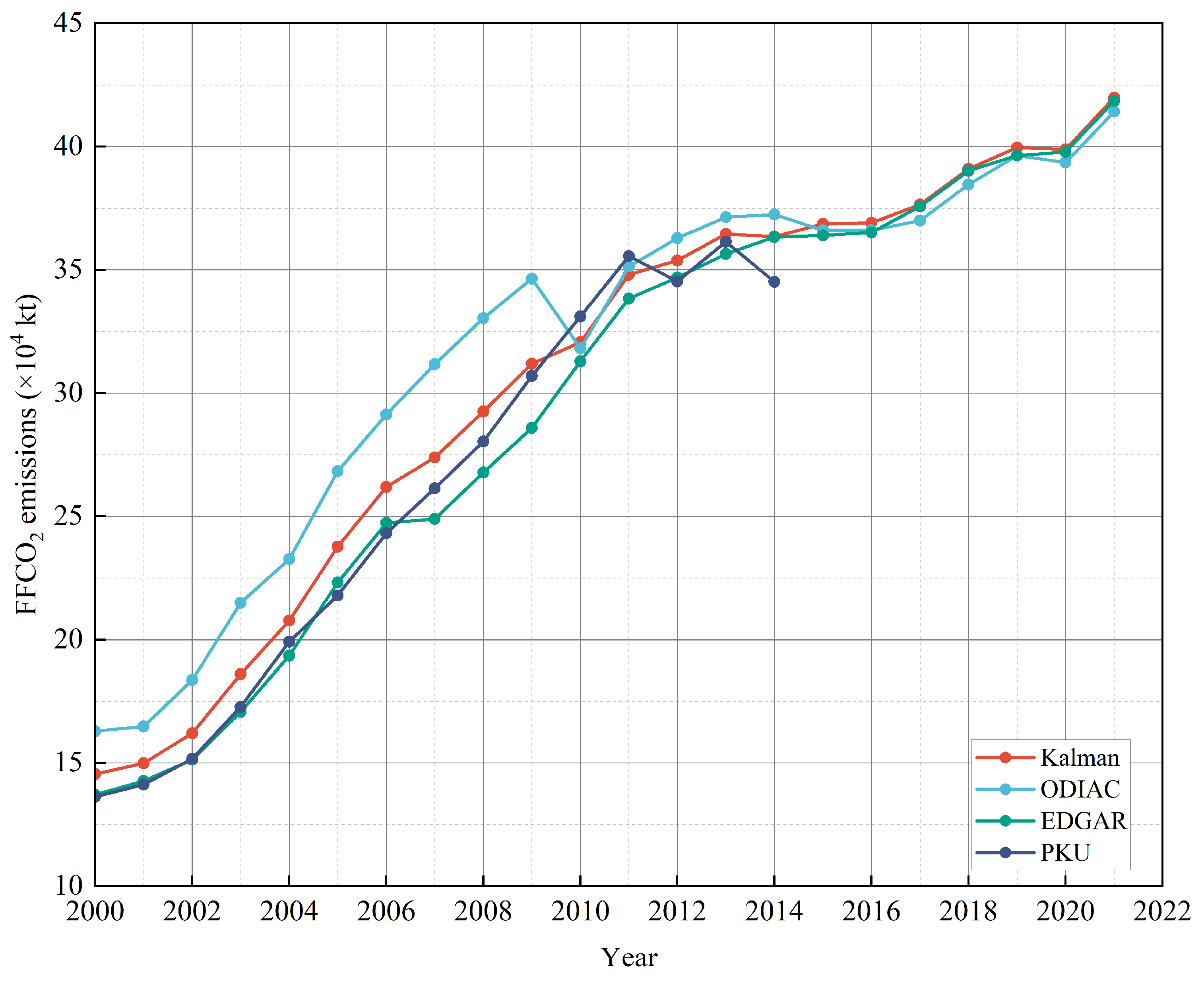
3.1. Kalman Fusion Results of Temporal Trends in FFCO₂ Emissions

Comparing biases between ODIAC, EDGAR, and PKU, we found that the smallest bias with a spatial resolution of 3 km × 3 km is optimally characterized in the GBA. Figure 3 illustrates the long–term trend of Kalman filter–fused FFCO₂ emissions in the GBA from 2000 to 2021, along with a comparison to ODIAC, EDGAR, and PKU. The fusion results for 2000–2014 are based on three datasets. As PKU data are only available up to 2014, the fusion results for 2015–2021 are reconstructed using ODIAC and EDGAR data only. Over the 21 years, FFCO₂ emissions in the GBA have shown a continuous increase, with a faster rate of increase in the first decade compared to the last decade. This trend is consistent with the global fossil CO₂ emissions reported by the Global Carbon Project (GCP) [58]. Specifically: (1) From 2000 to 2009, the Kalman fusion results increased from 145.48 Mt in 2000 to 311.93 Mt in 2009, closest to PKU’s FFCO₂ emissions. These values were significantly lower than ODIAC’s (14.97~37.82 Mt) and higher than EDGAR’s (7.18~26.09 Mt) during 2007–2009; A 1.4% decrease occurred during the global financial crisis [59], reflected only in ODIAC. The Kalman fusion results, EDGAR, and PKU continued to grow by 2.80%, 9.49%, and 7.87%, respectively. (2) Between 2010 and 2014, PKU’s FFCO₂ emissions exhibited a decreasing trend of 2.90% and 4.50% in 2012 and 2014, while the Kalman fusion results gradually aligned with ODIAC and EDGAR, showing similar trends and values, with a maximum deviation of 9.73 Mt. (3) Post–2015, the Kalman fusion results followed a similar trend to EDGAR and ODIAC, demonstrating greater data stability. Notably, during the 8.8% decrease in 2020 due to COVID-19 restrictions [50], ODIAC showed the most prominent decline (0.73%), followed by the Kalman fusion results (0.19%), with a slight increase in EDGAR (0.37%).

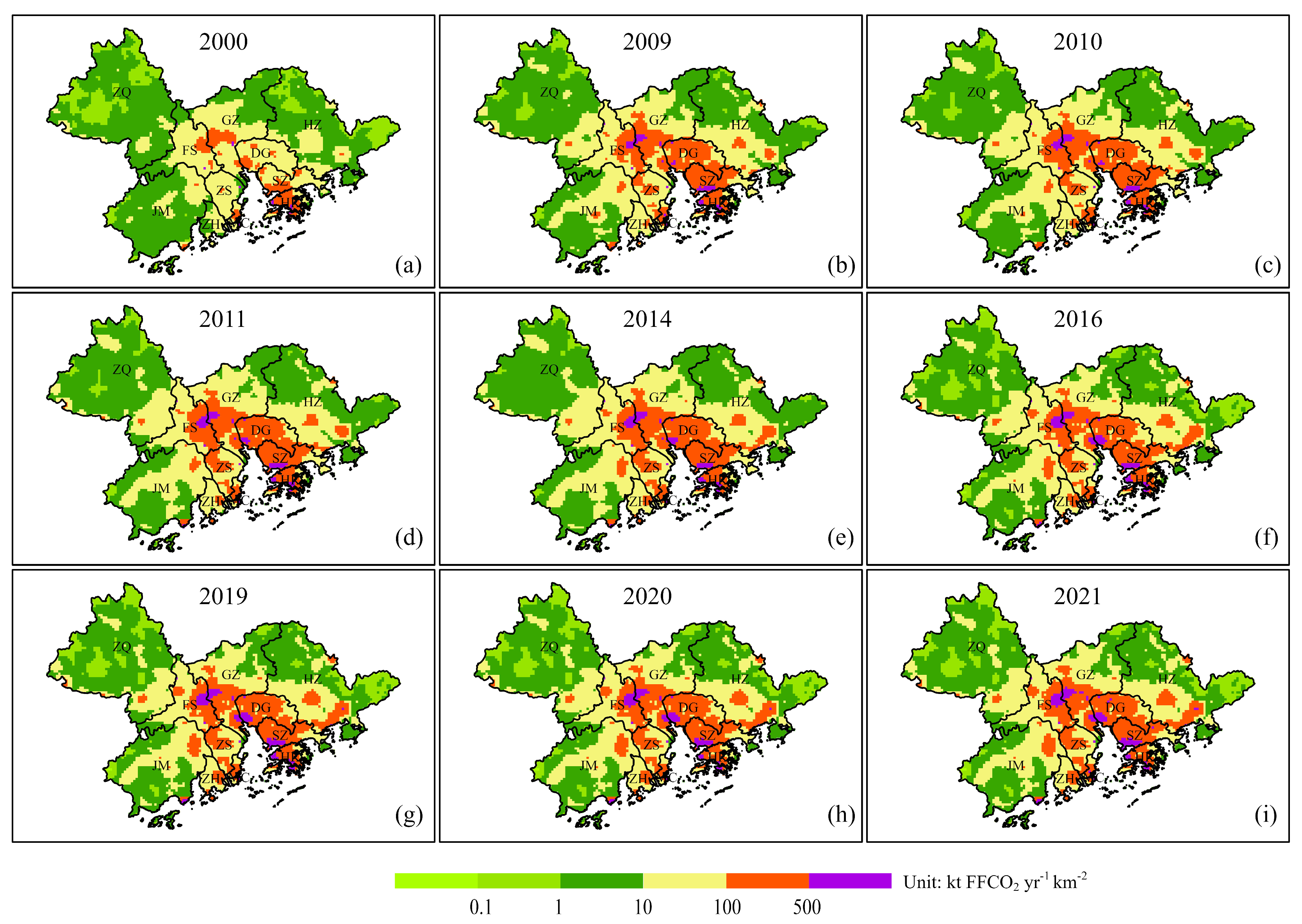
3.2. Kalman Fusion Results of FFCO₂ Spatial Distribution

Figure 4 illustrates the spatial distribution of Kalman filter–fused FFCO₂ emissions in the GBA for the years 2000, 2009, 2010, 2011, 2014, 2016, 2019, 2020, and 2021. These selected years capture significant changes in emissions patterns over time. Before fusion, the uncertainties (standard deviation) of ODIAC, EDGAR, and PKU were ±17.5%, ±15%, and ±19%, respectively. Post–fusion, the uncertainties of the Kalman fusion results for the periods 2000–2014 and 2015–2021 are reduced to ±9.77% and 11.39%, respectively, enhancing data accuracy and enabling a more precise characterization of spatial and temporal FFCO₂ emission patterns in the GBA at a regional scale. The spatial distribution of FFCO₂ emissions in the GBA over the 21–year period reveals a consistent trend: high–emission zones centered around core cities (GZ, SZ, HK, and MC) and key node cities (FS, DG, ZH, ZS) gradually tapering towards lower–emission zones at the periphery, encompassing other key node cities (ZQ, JM, HZ). This regional development pattern showcases the leadership role of central cities over key nodes. Moreover, the spatial distribution demonstrates an overall annual growth trend, aligning with the findings in Figure 3. Over the 21–year span, FFCO₂ emissions escalated from below 100 kt yr⁻¹ km⁻² in most cities (except HK) to exceeding 500 kt yr⁻¹ km⁻² in some areas of some cities (HK, GZ, FS, DG, and SZ). In particular, in 2000, almost all the cities in the GBA had FFCO₂ emissions below 100 kt yr⁻¹ km⁻², except for the whole region of HK and parts of GZ, FS, DG, and SZ, where emissions were 100 kt yr⁻¹ km⁻², and only sporadic locations had emissions above 500 kt yr⁻¹ km⁻²; by 2009, compared with the spatial distribution in 2000, large areas with emissions exceeding 500 kt yr⁻¹ km⁻² appeared in the core cities of the GZ–SZ border, in the southern part of SZ, and the eastern and southern parts of Hong Kong, while the areas in the emission range (10~500 kt yr⁻¹ km⁻²) were clearly spreading out in all directions. In the following decade or so, the spatial distribution of the high–value emission zones did not differ, although the trend of the regional average value continued to rise slowly. The objective here is to illustrate the distribution of exceptionally high values (exceeding 500 kt yr⁻¹ km⁻²) in the figure. By selecting 300 kt yr⁻¹ km⁻² as the dividing line, we can observe the outward diffusion characteristics of the purple highest value.

4. Discussion

4.1. Validation, Connecting Scales, and Uncertainties from Transferring Information from National to Local

Significant relative differences in emissions estimates from four widely used global inventories have been observed at regional (20%) and city scales (50–250%) [26]. In fact, over half of the grid cells in the 0.1° domain exhibit differences exceeding 100%, with the most substantial disparities occurring in urban areas and regions associated with oil and gas production. Spatial emission patterns also display considerable variations (10–100% relative difference at 1 km), particularly in urban–rural transition zones (90–100%) [16]. An analysis of the relative percentage error of grid cells at a 3 km resolution reveals an average variability of 140% within the Greater Bay Area (GBA). More than half of the grids exhibit a variability exceeding 130%, while over three–quarters demonstrate a variability greater than 80%. Additionally, the coefficient of variation (CV) for emission grids in the GBA ranges from 6% to 94% at resolutions between 0.5 and 5 km. Our reconstruction results account for these differences and variability. Notably, the ODIAC data exhibit significant instability and consistent deviations from EDGAR and PKU at resolutions of 0.5–5 km, as depicted in Figure 5a, corroborating findings from prior studies [36]. These results underscore the prevailing uncertainties in fossil fuel CO₂ (FFCO₂) inventories at the regional scale [15,27,37,60] and emphasize the importance of considering global–regional–scale linkages when reconstructing inventory data. Our analysis indicates that the optimal spatial resolution for reconstructing FFCO₂ emissions in the GBA is 3 km × 3 km, with the smallest deviation ranging from 0.12 to 63.84 Mt. This finding partially alleviates concerns raised in previous studies [26,61], as the significant uncertainties in these inventories do not provide entirely accurate representations of FFCO₂ emissions at subnational or urban scales. Moreover, it offers a relatively reliable solution in the absence of other directly observed emissions data.

To validate the accuracy and reliability of the reconstructed emissions, we compared them with the Carbon Budget (see Figure 5b) and GRACED emission data (see Figure 5c–f). Over the 21–year period at the global scale, the reconstructed results and the Carbon Budget assessment exhibit a convergence over time, demonstrating a high correlation of 0.99. Both datasets reflect the impact of significant global events that have imposed constraints on human activities and global CO₂ emissions. Notably, since 2014, the reconstructed results have fluctuated marginally above and below the Carbon Budget assessment due to the absence of PKU data. At the regional scale, the correlation coefficient between the Kalman fusion results and the GRACED emissions reaches 73% when considering the annual emission values of the 11 major cities in the GBA. This confirms that our estimates in the GBA offer more accurate representations of FFCO₂ emissions at the urban scale compared to ODIAC and EDGAR, which exhibit correlation coefficients of 57% and 65%, respectively, for New York City [26]. To further assess the spatial accuracy of the reconstructed data, we compared them with GRACED emission data, which have a spatial resolution of 0.1° × 0.1° (derived from TROPOMI NO₂ column data modeling). The analysis revealed that between 2019 and 2021, over half of the grids exhibited an absolute difference in emissions of less than 7 kt C, while more than three–quarters of the grids showed an absolute difference of less than 40 kt C. Additionally, less than 10% of grids displayed an absolute difference exceeding 150 kt C. Large deviations (>100 kt C) were predominantly observed in the core cities, indicating that the reliability of our fusion results is comparable to that of GRACED [41,43]. These discrepancies may be attributed to the exclusion of domestic aviation, international aviation, and international shipping data sources in our fusion data.

4.2. City–Level Variation Pattern with Improved Estimates of FFCO₂ Emissions

To determine the Kalman fusion results at the city level and analyze the regular center–shift pattern of intercity emissions [62,63], we further estimated the FFCO₂ emissions of cities in the GBA during significant transition years, as illustrated in Figure 6. It is evident that prior to 2014, both the reconstruction results and the PKU data exhibit higher sensitivity to high–value emission zones. However, post–2014, the reconstruction results demonstrate similar sensitivities to high–value emission zones as ODIAC and EDGAR. This indicates that the reconstruction results can effectively capture the emission status of key cities in the GBA, revealing the shift in emission centers among cities. Overall, the FFCO₂ emissions of all 11 cities in the GBA exhibit an upward trend over the 21–year period, aligning with previous research findings [64,65]. This trend contradicts the notion that emissions peaked in 2016 and subsequently declined annually [62]. Our results suggest a temporary growth slowdown between 2014 and 2016, followed by a sustained increase in emissions.

In terms of individual cities, particularly among the core cities, Macao SAR has consistently been identified as a high–emission area, yet its total urban emissions have remained relatively low due to its small footprint. Among the other core cities (GZ, SZ, HK), GZ has consistently emerged as the largest contributor [62,65,66] to emissions over the 21–year period, with emissions escalating from 29.76 Mt in 2000 to 82.21 Mt in 2021. While HK and SZ held the second and third positions in 2000, this trend underscores the transformation of core cities into major emission hubs, driven by factors such as favorable geographical positioning, advanced economic development, high urbanization rates, robust industrial configurations, and technological innovation [67,68]. By 2009, a shift in emissions focus had already begun. While SZ, the former third–largest emitting city, has retained its position, key node cities like FS and DG have experienced rapid emission growth, particularly DG, which has ascended to become the second–largest emitting city. The strategic geographical location of DG, positioned between GZ and HK, exposes it to the directional shift of carbon emissions from southeast to northwest. Additionally, changes in urban morphology significantly influence the carbon emissions of counties within DG. The emissions of other key node cities like HZ and ZS have also surged, surpassing those of Hong Kong in 2010. From 2011 to 2021, HK’s emission levels have consistently ranked seventh, attributed to the city’s adoption of optimized economic development models and stringent environmental protection measures in alignment with emission reduction policies [69]. Conversely, other key node cities like JM and ZH have exhibited lower emissions over the 21–year period due to their distance from economic hubs, relative industrial and energy structures, limited heavy industrial presence, and less–developed high–tech facilities. It is noteworthy that ZH, despite its advantageous geographic positioning, has only experienced a modest increase in FFCO₂ emissions (12.02 Mt) over the 21–year period. In late 2014, ZH was designated as a pilot demonstration city for low–carbon ecological collaboration between China and the European Union. As the sole city in Guangdong province to receive this distinction, ZH’s policy initiatives serve as a model for emulation in promoting sustainable practices.

4.3. FFCO₂ Emission Contributors by Urban–Rural Divide

In the context of shifting FFCO₂ emissions within the GBA over time, the conventional ‘core–periphery’ pattern [67] may no longer serve as the most reliable indicator of transition or cross–border emission dynamics. To better understand these changes, we delineated the Urban–Rural Divide within GBA lands based on 10 m Esri Sentinel–2 Land Cover Type data, categorizing regions into ‘Urban’, ‘Suburban’, and ‘Rural’ areas. Concurrently, we integrated spatio–temporal socio–economic data (NTL, GDP, POP) to gain insights into the sources of emissions at the urban–rural interface (refer to Figure 1b). Using the Urban–Rural Divide as a mask, we conducted a comprehensive analysis employing multiple regression analysis to assess the contributions of factors such as GDP, POP, and energy consumption (EC) which can be indirectly inferred from NTL data [70], to emissions in urban, suburban, and rural areas of the GBA. Our findings, illustrated in Figure 7, reveal intriguing trends in the sensitivity of FFCO₂ emission formation based on the aforementioned contributors over time. From 2000 to 2009, there was a notable increase in the share of EC–contributed emissions across the GBA, followed by a decline from 2011 to 2019. This decline aligns with heightened restrictions and controls on energy consumption, indicating a positive impact on reducing FFCO₂ emissions regionally. However, a contrasting pattern emerged in urban areas, where the proportion of EC–contributed emissions exhibited fluctuations, suggesting challenges in effectively curbing urban energy consumption despite ongoing emission reduction policies. Interestingly, suburban areas maintained a relatively stable share of EC–contributed emissions, while rural regions experienced a decline, possibly reflecting a trend of rural–to–urban migration within the GBA. The diminishing role of energy consumption and population [71] in rural emissions underscores the shifting dynamics within the region. Moreover, our analysis highlights the significant influence of energy consumption on suburban emissions, with GDP playing a more prominent role in suburban areas compared to their urban and rural counterparts. Notably, suburbs located in peripheral cities like ZQ, HZ, and JM demonstrate a balanced interplay between GDP and energy consumption effects over the 21–year period. This approach and these findings quantitatively estimate the relevance of different development levels of Urban–Rural Divides to specific human activities or emission sources, explore cross–border emission dynamics. However, they imply the intricate interplay of socio–economic factors in driving emissions patterns within the GBA. It is therefore recommended that more high–precision data and targeted strategies be employed to address the evolving dynamics of urban–rural emissions.

5. Conclusions

This study utilized a variety of monitoring and reanalysis data spanning from 2000 to 2021 for the GBA, China. The aim was to develop an optimal regional spatial resolution product for FFCO₂ emissions and enhance our understanding of the regional–scale spatio–temporal dynamics of these emissions. To address uncertainties among the three selected global–scale inventories in the GBA, a comparison and quantification of relative differences and CVs were incorporated into the reconstruction algorithm. A Kalman filter fusion method was then employed to reconcile errors between inventories and reduce uncertainties in their spatial characteristics at the regional scale, resulting in a new regional FFCO₂ emission product that bridges the global and regional scales. The accuracy and reliability of the reconstructed emissions in the GBA were further validated using real–time data and an Urban–Rural Divide approach to analyze spatio–temporal variation patterns, conduct a city–level cross–validation, and identify emissions contributors. The empirical findings and conclusions are summarized as follows.

Significant differences and CVs are observed among the inventories, particularly at the regional and urban scales. The ODIAC inventory exhibits notable instability and consistent deviations from EDGAR and PKU within the range of 0.5–5 km, with the smallest deviation occurring at a 3 km × 3 km resolution. Grid cell variability in the three global emission inventories in the GBA reaches up to 140%, with over half of the grid cells showing a variability greater than 130% and more than three–quarters exceeding 80% at 3 km resolution. The CV of emission grids within the 0.5–5 km range varies from 6% to 94%. Consequently, reconstructing the inventories offers a more reliable method for determining the optimal spatial resolution with minimal deviation by linking global and regional scales, when direct emissions data are unavailable.

Prior to reconstruction, uncertainties in the ODIAC, EDGAR, and PKU inventories were ±17.5%, ±15%, and ±19%, respectively. Following the reconstruction, the uncertainties in the Kalman fusion results for the periods 2000–2014 and 2015–2021 were reduced to ±9.77% and ±11.39%, significantly enhancing data accuracy, to better depict the spatial and temporal patterns of FFCO₂ emissions in the GBA at the regional scale. Our estimates for FFCO₂ emissions in the GBA offer a more precise reflection (73%) of urban–scale emissions compared to ODIAC (57%) and EDGAR (65%) estimates for New York City. Temporally, FFCO₂ emissions in the GBA have shown a consistent upward trend over the 21–year period, with a faster increase in the first decade compared to the last. The result does not show a decline in 2010, but rather an increase of 2.8%, influenced by the global financial crisis. Nevertheless, the results demonstrate a notable decline of 0.19% due to the implementation of restrictions associated with the global pandemic in 2020. Spatially, a “core–subcore–periphery” pattern emerges, with economically robust cities such as GZ, SZ, HK, and MC at the core, less developed cities like FS, DG, ZH, and ZS at the subcore, and least developed cities like ZQ, JM, and HZ on the periphery.

The temporal evolution of the center–shift of the “core–subcore–periphery” pattern was investigated through a city cross–variation analysis and contributors from the Urban–Rural Divide. The FFCO₂ emissions of all 11 cities in the GBA exhibited a consistent upward trend over a 21–year period. While there was a brief slowdown in growth between 2014 and 2016, emissions continued to rise thereafter. The core city GZ consistently emerges as the largest contributor to emissions throughout the 21–year period. By 2009, a noticeable shift in emission centers had already begun. SZ, previously the third–largest emitter, maintained its position, with subcore cities like FS and DG experiencing rapid emission growth, particularly DG, which ascended to become the second–largest emitting city. Starting from 2011, HK transitioned to the seventh–highest emitter position. The main drivers behind the center–shift of the “core–subcore–periphery” pattern include the urban layout of the 11 cities, influence from neighboring core cities, rural–to–urban population migration, and the significant contribution of GDP from suburban areas. Notably, there was no significant correlation found with electricity consumption

Given the pressing nature of the current decarbonization challenge, it is critical for policymakers to rigorously evaluate the accuracy of foundational data, the spatio–temporal dynamics of “core–subcore–periphery” emissions, the center–shift of the pattern, and the key influencing contributors. This scrutiny will bolster the precision of decision–making processes and expedite the decarbonization endeavor. In future studies, it is recommended to integrate satellite CO₂ observations with emission inventories to validate the “core–subcore–periphery” emission pattern in the GBA. While current satellite data may not yet be optimal for urban–scale emission research, preliminary investigations can leverage multi–source satellite observations in conjunction with atmospheric chemistry models. Subsequent research endeavors should focus on identifying relevant driving factor variables, conducting quantitative analyses of the driving mechanisms using appropriate models and research methodologies, and undertaking a systematic and comprehensive examination of the underlying motivations behind the temporal and spatial evolution of carbon emissions in the GBA.

References

1. IPCC. Climate Change 2014—Impacts, Adaptation and Vulnerability: Part A: Global and Sectoral Aspects; Cambridge University Press: Cambridge, UK; New York, NY, USA, 2014. [Google Scholar]
2. Crippa, M.; Guizzardi, D.; Muntean, M.; Schaaf, E.; Solazzo, E.; Monforti-Ferrario, F.; Olivier, J.G.J.; Vignati, E. Fossil CO2 Emissions of all World Countries: 2020 Report; Publications Office of the European Union: Luxembourg, 2020. [Google Scholar]
3. Lei, R.; Feng, S.; Danjou, A.; Broquet, G.; Wu, D.; Lin, J.C.; O’Dell, C.W.; Lauvaux, T. Fossil fuel CO2 emissions over metropolitan areas from space: A multi-model analysis of OCO-2 data over Lahore, Pakistan. Remote Sens. Environ. 2021, 264, 112625. [Google Scholar] [CrossRef]
4. Che, K.; Cai, Z.; Liu, Y.; Wu, L.; Yang, D.; Chen, Y.; Meng, X.; Zhou, M.; Wang, J.; Yao, L.; et al. Lagrangian inversion of anthropogenic CO2 emissions from Beijing using differential column measurements. Environ. Res. Lett. 2022, 17, 75001. [Google Scholar] [CrossRef]
5. Huang, C.; Zhuang, Q.; Meng, X.; Zhu, P.; Han, J.; Huang, L. A fine spatial resolution modeling of urban carbon emissions: A case study of Shanghai, China. Sci. Rep. 2022, 12, 9255. [Google Scholar] [CrossRef] [PubMed]
6. IPCC. Climate Change 2022: Mitigation of Climate Change. Contribution of Working Group III to the Sixth Assessment Report of the Intergovernmental Panel on Climate Change; Cambridge University Press: Cambridge, UK; New York, NY, USA, 2022. [Google Scholar]
7. Liu, J.; Li, H.; Liu, T. Decoupling Regional Economic Growth from Industrial CO2 Emissions: Empirical Evidence from the 13 Prefecture-Level Cities in Jiangsu Province. Sustainability 2022, 14, 2733. [Google Scholar] [CrossRef]
8. Liu, K.; Ni, Z.Y.; Ren, M.; Zhang, X.Q. Spatial Differences and Influential Factors of Urban Carbon Emissions in China under the Target of Carbon Neutrality. Int. J. Environ. Res. Public Health 2022, 19, 6427. [Google Scholar] [CrossRef] [PubMed]
9. UNFCCC. Paris Agreement; UNFCCC: Rio de Janeiro, Brazil; New York, NY, USA, 2015. [Google Scholar]
10. Andersen, K.S.; Termansen, L.B.; Gargiulo, M.; Ó Gallachóirc, B.P. Bridging the gap using energy services: Demonstrating a novel framework for soft linking top-down and bottom-up models. Energy 2019, 169, 277–293. [Google Scholar] [CrossRef]
11. Lombardi, M.; Laiola, E.; Tricase, C.; Rana, R. Assessing the urban carbon footprint: An overview. Environ. Impact Assess. Rev. 2017, 66, 43–52. [Google Scholar] [CrossRef]
12. Pisso, I.; Patra, P.; Takigawa, M.; Machida, T.; Matsueda, H.; Sawa, Y. Assessing Lagrangian inverse modelling of urban anthropogenic CO2 fluxes using in situ aircraft and ground-based measurements in the Tokyo area. Carbon Balance Manag. 2019, 14, 6699. [Google Scholar] [CrossRef] [PubMed]
13. Maksyutov, S.; Brunner, D.; Turner, A.J.; Zavala-Araiza, D.; Janardanan, R.; Bun, R.; Oda, T.; Patra, P.K. Applications of top-down methods to anthropogenic GHG emission estimation. In Balancing Greenhouse Gas Budgets; Elsevier: Amsterdam, The Netherlands, 2022; pp. 455–481. ISBN 9780128149522. [Google Scholar]
14. Pitt, J.R.; Lopez-Coto, I.; Hajny, K.D.; Tomlin, J.; Kaeser, R.; Jayarathne, T.; Stirm, B.H.; Floerchinger, C.R.; Loughner, C.P.; Gately, C.K.; et al. New York City greenhouse gas emissions estimated with inverse modeling of aircraft measurements. Elem. Sci. Anthr. 2022, 10, 00082. [Google Scholar] [CrossRef]
15. Gurney, K.R.; Liang, J.; O’Keeffe, D.; Patarasuk, R.; Hutchins, M.; Huang, J.; Rao, P.; Song, Y. Comparison of Global Downscaled Versus Bottom-Up Fossil Fuel CO2 Emissions at the Urban Scale in Four U.S. Urban Areas. J. Geophys. Res. Atmos. 2019, 124, 2823–2840. [Google Scholar] [CrossRef]
16. Oda, T.; Bun, R.; Kinakh, V.; Topylko, P.; Halushchak, M.; Marland, G.; Lauvaux, T.; Jonas, M.; Maksyutov, S.; Nahorski, Z.; et al. Errors and uncertainties in a gridded carbon dioxide emissions inventory. Mitig. Adapt. Strat. Glob. Chang. 2019, 24, 1007–1050. [Google Scholar] [CrossRef]
17. Li, M.; Zhang, Q.; Kurokawa, J.; Woo, J.-H.; He, K.; Lu, Z.; Ohara, T.; Song, Y.; Streets, D.G.; Carmichael, G.R.; et al. MIX: A mosaic Asian anthropogenic emission inventory under the international collaboration framework of the MICS-Asia and HTAP. Atmos. Chem. Phys. 2017, 17, 935–963. [Google Scholar] [CrossRef]
18. Zhang, L.; Long, R.; Chen, H.; Yang, T. Analysis of an optimal public transport structure under a carbon emission constraint: A case study in Shanghai, China. Environ. Sci. Pollut. Res. Int. 2018, 25, 3348–3359. [Google Scholar] [CrossRef] [PubMed]
19. Oda, T.; Maksyutov, S.; Andres, R.J. The Open-source Data Inventory for Anthropogenic Carbon dioxide (CO2), version 2016 (ODIAC2016): A global, monthly fossil-fuel CO2 gridded emission data product for tracer transport simulations and surface flux inversions. Earth Syst. Sci. Data 2018, 10, 87–107. [Google Scholar] [CrossRef] [PubMed]
20. Wang, Y.; Li, G. Mapping urban CO2 emissions using DMSP/OLS ‘city lights’ satellite data in China. Environ. Plan. A 2017, 49, 248–251. [Google Scholar] [CrossRef]
21. Wang, R.; Tao, S.; Ciais, P.; Shen, H.Z.; Huang, Y.; Chen, H.; Shen, G.F.; Wang, B.; Li, W.; Zhang, Y.Y.; et al. High-resolution mapping of combustion processes and implications for CO2 emissions. Atmos. Chem. Phys. 2013, 13, 5189–5203. [Google Scholar] [CrossRef]
22. Gurney, K.R.; Razlivanov, I.; Song, Y.; Zhou, Y.; Benes, B.; Abdul-Massih, M. Quantification of fossil fuel CO2 emissions on the building/street scale for a large U.S. city. Environ. Sci. Technol. 2012, 46, 12194–12202. [Google Scholar] [CrossRef] [PubMed]
23. Gurney, K.R.; Liang, J.; Roest, G.; Song, Y.; Mueller, K.; Lauvaux, T. Under-reporting of greenhouse gas emissions in U.S. cities. Nat. Commun. 2021, 12, 16083. [Google Scholar] [CrossRef] [PubMed]
24. Macknick, J. Energy and CO2 emission data uncertainties. Carbon Manag. 2011, 2, 189–205. [Google Scholar] [CrossRef]
25. Hogue, S.; Marland, E.; Andres, R.J.; Marland, G.; Woodard, D. Uncertainty in gridded CO2 emissions estimates. Earth’s Fut. 2016, 4, 225–239. [Google Scholar] [CrossRef]
26. Gately, C.K.; Hutyra, L.R. Large Uncertainties in Urban-Scale Carbon Emissions. J. Geophys. Res. Atmos. 2017, 122, 1. [Google Scholar] [CrossRef]
27. Han, P.; Zeng, N.; Oda, T.; Zhang, W.; Lin, X.; Liu, D.; Cai, Q.; Ma, X.; Meng, W.; Wang, G.; et al. A city-level comparison of fossil-fuel and industry processes-induced CO2 emissions over the Beijing-Tianjin-Hebei region from eight emission inventories. Carbon Balance Manag. 2020, 15, 25. [Google Scholar] [CrossRef] [PubMed]
28. Lauvaux, T.; Gurney, K.R.; Miles, N.L.; Davis, K.J.; Richardson, S.J.; Deng, A.; Nathan, B.J.; Oda, T.; Wang, J.A.; Hutyra, L.; et al. Policy-Relevant Assessment of Urban CO2 Emissions. Environ. Sci. Technol. 2020, 54, 10237–10245. [Google Scholar] [CrossRef] [PubMed]
29. NDRC. Action Plan for Carbon Dioxide Peaking Before 2030. 2021. Available online: https://en.ndrc.gov.cn/policies/202110/t20211027_1301020.html (accessed on 5 April 2024).
30. Green, F.; Stern, N. China’s changing economy: Implications for its carbon dioxide emissions. Clim. Policy 2017, 17, 423–442. [Google Scholar] [CrossRef]
31. The State Council of the People’s Republic of China. Guangdong-Hong Kong-Macau Greater Bay Area Development Plan Outline; The State Council of the People’s Republic of China: Beijing, China, 2019. [Google Scholar]
32. Yona, L.; Cashore, B.; Jackson, R.B.; Ometto, J.; Bradford, M.A. Refining national greenhouse gas inventories. Ambio 2020, 49, 1581–1586. [Google Scholar] [CrossRef] [PubMed]
33. Crippa, M.; Guizzardi, D.; Banja, M.; Solazzo, E.; Muntean, M.; Schaaf, E.; Pagani, F.; Monforti-Ferrario, F.; Olivier, J.; Quadrelli, R.; et al. CO2 Emissions of All World Countries—JRC/IEA/PBL 2022 Report; JRC130363; Publications Office of the European Union: Luxembourg, 2022. [Google Scholar] [CrossRef]
34. Crippa, M.; Guizzardi, D.; Pagani, F.; Banja, M.; Muntean, M.; Schaaf, E.; Becker, W.; Monforti-Ferrario, F.; Quadrelli, R.; Risquez Martin, A.; et al. GHG Emissions of All World Countries; Publications Office of the European Union: Luxembourg, 2023; Available online: https://op.europa.eu/en/publication-detail/-/publication/0cde0e23-5057-11ee-9220-01aa75ed71a1/language-en (accessed on 5 April 2024).
35. Chevallier, F.; Broquet, G.; Zheng, B.; Ciais, P.; Eldering, A. Large CO2 Emitters as Seen From Satellite: Comparison to a Gridded Global Emission Inventory. Geophys. Res. Lett. 2022, 49, e2021GL097540. [Google Scholar] [CrossRef] [PubMed]
36. Zhao, J.; Cohen, J.B.; Chen, Y.T.; Cui, W.H.; Cao, Q.Q.; Yang, T.F.; Li, G.Q. High-resolution spatiotemporal patterns of China’s FFCO2 emissions under the impact of LUCC from 2000 to 2015. Environ. Res. Lett. 2020, 15, 44007. [Google Scholar] [CrossRef]
37. Ahn, D.Y.; Goldberg, D.L.; Coombes, T.; Kleiman, G.; Anenberg, S.C. CO2 emissions from C40 cities: Citywide emission inventories and comparisons with global gridded emission datasets. Environ. Res. Lett. 2023, 18, 34032. [Google Scholar] [CrossRef] [PubMed]
38. Román, M.O.; Wang, Z.; Sun, Q.; Kalb, V.; Miller, S.D.; Molthan, A.; Schultz, L.; Bell, J.; Stokes, E.C.; Pandey, B.; et al. NASA’s Black Marble nighttime lights product suite. Remote Sens. Environ. 2018, 210, 113–143. [Google Scholar] [CrossRef]
39. Hefner, M.; Marland, G. Global, Regional, and National Fossil-Fuel CO2 Emissions: 1751-2020 CDIAC-FF; Research Institute for Environment, Energy, and Economics, Appalachian State University. Available online: https://energy.appstate.edu/research/work-areas/cdiac-appstate (accessed on 5 April 2024).
40. Tao, M.; Cai, Z.; Che, K.; Liu, Y.; Yang, D.; Wu, L.; Wang, P.; Yang, M. Cross-Inventory Uncertainty Analysis of Fossil Fuel CO2 Emissions for Prefecture-Level Cities in Shandong Province. Atmosphere 2022, 13, 1474. [Google Scholar] [CrossRef]
41. Dou, X.; Hong, J.; Ciais, P.; Chevallier, F.; Yan, F.; Yu, Y.; Hu, Y.; Da, H.; Sun, Y.; Wang, Y.; et al. Near-real-time global gridded daily CO2 emissions 2021. Sci. Data 2023, 10, 69. [Google Scholar] [CrossRef] [PubMed]
42. Liu, Z.; Ciais, P.; Deng, Z.; Davis, S.J.; Zheng, B.; Wang, Y.; Cui, D.; Zhu, B.; Dou, X.; Ke, P.; et al. Carbon Monitor, a near-real-time daily dataset of global CO2 emission from fossil fuel and cement production. Sci. Data 2020, 7, 392. [Google Scholar] [CrossRef] [PubMed]
43. Dou, X.; Wang, Y.; Ciais, P.; Chevallier, F.; Davis, S.J.; Crippa, M.; Janssens-Maenhout, G.; Guizzardi, D.; Solazzo, E.; Yan, F.; et al. Near-real-time global gridded daily CO2 emissions. Innovation 2022, 3, 100182. [Google Scholar] [CrossRef] [PubMed]
44. Monforti Ferrario, F.; Crippa, M.; Guizzardi, D.; Muntean, M.; Schaaf, E.; Lo Vullo, E.; Solazzo, E.; Olivier, J.; Vignati, E. EDGAR v6.0 Greenhouse Gas Emissions. European Commission. Available online: https://data.jrc.ec.europa.eu/dataset/97a67d67-c62e-4826-b873-9d972c4f670b (accessed on 28 June 2023).
45. Janssens-Maenhout, G.; Crippa, M.; Guizzardi, D.; Muntean, M.; Schaaf, E.; Dentener, F.; Bergamaschi, P.; Pagliari, V.; Olivier, J.G.J.; Peters, J.A.H.W.; et al. EDGAR v4.3.2 Global Atlas of the three major greenhouse gas emissions for the period 1970–2012. Earth Syst. Sci. Data 2019, 11, 959–1002. [Google Scholar] [CrossRef]
46. Crippa, M.; Guizzardi, D.; Pisoni, E.; Solazzo, E.; Guion, A.; Muntean, M.; Florczyk, A.; Schiavina, M.; Melchiorri, M.; Hutfilter, A.F. Global anthropogenic emissions in urban areas: Patterns, trends, and challenges. Environ. Res. Lett. 2021, 16, 74033. [Google Scholar] [CrossRef]
47. Oda, T.; Maksyutov, S. A very high-resolution (1 km × 1 km) global fossil fuel CO2 emission inventory derived using a point source database and satellite observations of nighttime lights. Atmos. Chem. Phys. 2011, 11, 543–556. [Google Scholar] [CrossRef]
48. Liu, Z.; Guan, D.; Wei, W.; Davis, S.J.; Ciais, P.; Bai, J.; Peng, S.; Zhang, Q.; Hubacek, K.; Marland, G.; et al. Reduced carbon emission estimates from fossil fuel combustion and cement production in China. Nature 2015, 524, 335–338. [Google Scholar] [CrossRef] [PubMed]
49. Chen, H.; Huang, Y.; Shen, H.; Chen, Y.; Ru, M.; Chen, Y.; Lin, N.; Su, S.; Zhuo, S.; Zhong, Q.; et al. Modeling temporal variations in global residential energy consumption and pollutant emissions. Appl. Energy 2016, 184, 820–829. [Google Scholar] [CrossRef]
50. Liu, Z.; Ciais, P.; Deng, Z.; Lei, R.; Davis, S.J.; Feng, S.; Zheng, B.; Cui, D.; Dou, X.; Zhu, B.; et al. Near-real-time monitoring of global CO2 emissions reveals the effects of the COVID-19 pandemic. Nat. Commun. 2020, 11, 5172. [Google Scholar] [CrossRef]
51. Chen, Z.; Yu, B.; Yang, C.; Zhou, Y.; Yao, S.; Qian, X.; Wang, C.; Wu, B.; Wu, J. An extended time series (2000–2018) of global NPP-VIIRS-like nighttime light data from a cross-sensor calibration. Earth Syst. Sci. Data 2021, 13, 889–906. [Google Scholar] [CrossRef]
52. Chen, J.; Gao, M.; Cheng, S.; Hou, W.; Song, M.; Liu, X.; Liu, Y. Global 1 km × 1 km gridded revised real gross domestic product and electricity consumption during 1992-2019 based on calibrated nighttime light data. Sci. Data 2022, 9, 202. [Google Scholar] [CrossRef] [PubMed]
53. Adjognon, G.S.; Rivera-Ballesteros, A.; van Soest, D. Satellite-based tree cover mapping for forest conservation in the drylands of Sub Saharan Africa (SSA): Application to Burkina Faso gazetted forests. Dev. Eng. 2019, 4, 100039. [Google Scholar] [CrossRef]
54. Naidoo, L.; van Deventer, H.; Ramoelo, A.; Mathieu, R.; Nondlazi, B.; Gangat, R. Estimating above ground biomass as an indicator of carbon storage in vegetated wetlands of the grassland biome of South Africa. Int. J. Appl. Earth Obs. Geoinf. 2019, 78, 118–129. [Google Scholar] [CrossRef]
55. Chen, Y.; Yan, H.; Yao, Y.; Zeng, C.; Gao, P.; Zhuang, L.; Fan, L.; Ye, D. Relationships of ozone formation sensitivity with precursors emissions, meteorology and land use types, in Guangdong-Hong Kong-Macao Greater Bay Area, China. J. Environ. Sci. 2020, 94, 1–13. [Google Scholar] [CrossRef] [PubMed]
56. Rayner, P.J.; Raupach, M.R.; Paget, M.; Peylin, P.; Koffi, E. A new global gridded data set of CO2 emissions from fossil fuel combustion: Methodology and evaluation. J. Geophys. Res. 2010, 115, D19306. [Google Scholar] [CrossRef]
57. Kalman, R.E. A New Approach to Linear Filtering and Prediction Problems. J. Basic Eng. 1960, 82, 35–45. [Google Scholar] [CrossRef]
58. Friedlingstein, P.; O’Sullivan, M.; Jones, M.W.; Andrew, R.M.; Bakker, D.C.E.; Hauck, J.; Landschützer, P.; Le Quéré, C.; Luijkx, I.T.; Peters, G.P.; et al. Global Carbon Budget 2023. Earth Syst. Sci. Data 2023, 15, 5301–5369. [Google Scholar] [CrossRef]
59. Peters, G.P.; Marland, G.; Le Quéré, C.; Boden, T.; Canadell, J.G.; Raupach, M.R. Rapid growth in CO2 emissions after the 2008–2009 global financial crisis. Nat. Clim. Chang. 2012, 2, 2–4. [Google Scholar] [CrossRef]
60. Kato, A.; Gurney, K.R.; Roest, G.S.; Dass, P. Exploring differences in FFCO2 emissions in the United States: Comparison of the Vulcan data product and the EPA national GHG inventory. Environ. Res. Lett. 2023, 18, 124043. [Google Scholar] [CrossRef]
61. Maier, F.M.; Levin, I.; Conil, S.; Gachkivskyi, M.; van der Denier Gon, H.; Hammer, S. Uncertainty of continuous ∆CO-based ∆ffCO2 estimates derived from 14C flask and bottom-up ∆CO/∆ffCO2 ratios. EGUsphere 2023, 2023, 1–31. [Google Scholar] [CrossRef]
62. Li, L.; Li, J.; Wang, X.; Sun, S. Spatio-temporal evolution and gravity center change of carbon emissions in the Guangdong-Hong Kong-Macao greater bay area and the influencing factors. Heliyon 2023, 9, e16596. [Google Scholar] [CrossRef] [PubMed]
63. Li, L.; Li, J.; Peng, L.; Wang, X.; Sun, S. Spatiotemporal evolution and influencing factors of land-use emissions in the Guangdong-Hong Kong-Macao Greater Bay Area using integrated nighttime light datasets. Sci. Total Environ. 2023, 893, 164723. [Google Scholar] [CrossRef] [PubMed]
64. Ming, L.; Wang, Y.; Chen, X.; Meng, L. Dynamics of urban expansion and form changes impacting carbon emissions in the Guangdong-Hong Kong-Macao Greater Bay Area counties. Heliyon 2024, 10, e29647. [Google Scholar] [CrossRef] [PubMed]
65. Zhou, Y.; Li, K.; Liang, S.; Zeng, X.; Cai, Y.; Meng, J.; Shan, Y.; Guan, D.; Yang, Z. Trends, Drivers, and Mitigation of CO2 Emissions in the Guangdong–Hong Kong–Macao Greater Bay Area. Engineering 2023, 23, 138–148. [Google Scholar] [CrossRef]
66. Lin, B.; Li, Z. Spatial analysis of mainland cities’ carbon emissions of and around Guangdong-Hong Kong-Macao Greater Bay area. Sustain. Cities Soc. 2020, 61, 102299. [Google Scholar] [CrossRef]
67. Wei, H.; Zheng, C. Spatial network structure and influencing factors of carbon emission intensity in Guangdong-Hong Kong-Macao greater bay area. Front. Environ. Sci. 2024, 12, 1380831. [Google Scholar] [CrossRef]
68. Liu, J.; Lo, K.; Mah, D.; Guo, M. Cross-Border Governance and Sustainable Energy Transition: The Case of the Guangdong-Hong Kong-Macao Greater Bay Area. Curr. Sustain./Renew. Energy Rep. 2021, 8, 101–106. [Google Scholar] [CrossRef]
69. Environment Bureau. Hong Kong’s Climate Action Plan 2030+; Environment Bureau: Hong Kong, China, 2017. [Google Scholar]
70. Mellander, C.; Lobo, J.; Stolarick, K.; Matheson, Z. Night-Time Light Data: A Good Proxy Measure for Economic Activity? PLoS ONE 2015, 10, e0139779. [Google Scholar] [CrossRef]
71. Wang, L.; Wu, Z.; Wang, X. Multimodal transportation and city carbon emissions over space and time: Evidence from Guangdong-Hong Kong-Macao Greater Bay Area, China. J. Clean. Prod. 2023, 425, 138987. [Google Scholar] [CrossRef]
Figure 1. The location, geographic scope, and Urban–Rural Divide of the GBA: (a) The GBA is comprised of 11 cities, including the core cities of Guangzhou (GZ), Shenzhen (SZ), Hong Kong (HK), and Macao (MC), as well as the key node cities of Foshan (FS), Dongguan (DG), Zhuhai (ZH), Zhongshan (ZS), Zhaoqing (ZQ), Jiangmen (JM), and Huizhou (HZ). (Note: ArcGIS Pro, Version 3.0.2, ESRI was utilized to create this figure). (b) Urban–Rural Divide in 2021 generated from land use cover of GBA.
Remotesensing 16 02354 g001
Figure 2. Flowchart of multi–source fusion for FFCO2 emission inventories at regional scale.
Remotesensing 16 02354 g002
Figure 3. Temporal trend of Kalman filter–fused FFCO2 emissions in GBA from 2000 to 2021, with comparison to ODIAC, EDGAR, and PKU.
Remotesensing 16 02354 g003
Figure 4. (ai) Kalman fusion results of FFCO2 spatial distribution (3 km) in GBA in 2000, 2009, 2010, 2011, 2014, 2016, 2019, 2020 and 2021.
Remotesensing 16 02354 g004
Figure 5. Scale verification of Kalman filter fusion results and comparison with Carbon Budget and GRACED data: (a) Scale effects and uncertainties in data sources before reconstruction. (b) Comparison of global and regional Kalman fusion results and Carbon Budget emissions from 2000 to 2021 (sampling annual emission values in the European Union, Africa, Asia, Central America, Europe, the Middle East, Oceania, South America, and North America). (c) Comparison of FFCO2 emissions between Kalman fusion results and GRACED CO2 emission estimates in GBA. (df) Spatial difference between Kalman integration results and GRACED CO2 emission estimates in GBA from 2019 to 2021.
Remotesensing 16 02354 g005
Figure 6. City–level variation pattern in nine important change years.
Remotesensing 16 02354 g006
Figure 7. Proportion variations of FFCO2 emission formation sensitivity in urban, suburban and rural areas of GBA, from 2000 to 2019.
Remotesensing 16 02354 g007
Disclaimer/Publisher’s Note: The statements, opinions and data contained in all publications are solely those of the individual author(s) and contributor(s) and not of MDPI and/or the editor(s). MDPI and/or the editor(s) disclaim responsibility for any injury to people or property resulting from any ideas, methods, instructions or products referred to in the content.