Exterior Orientation Parameter Refinement of the First Chinese Airborne Three-Line Scanner Mapping System AMS-3000

Abstract

The exterior orientation parameters (EOPs) provided by the self-developed position and orientation system (POS) of the first Chinese airborne three-line scanner mapping system, AMS-3000, are impacted by jitter, resulting in waveform distortions in rectified images. This study introduces a Gaussian Markov EOP refinement method enhanced by cubic spline interpolation to mitigate stochastic jitter errors. Our method first projects tri-view images onto a mean elevation plane using POS-provided EOPs to generate Level 1 images for dense matching. Matched points are then back-projected to the original Level 0 images for the bundle adjustment based on the Gaussian Markov model. Finally, cubic spline interpolation is employed to obtain EOPs for lines without observations. Experimental comparisons with the piecewise polynomial model (PPM) and Lagrange interpolation model (LIM) demonstrate that our method outperformed these models in terms of geo-referencing accuracy, EOP refinement metric, and visual performance. Specifically, the line fitting accuracies of four linear features on Level 1 images were evaluated to assess EOP refinement performance. The refinement performance of our method showed improvements of 50%, 45.1%, 29.9%, and 44.6% over the LIM, and 12.9%, 69.2%, 69.6%, and 49.3% over the PPM. Additionally, our method exhibited the best visual performance on these linear features.

1. Introduction

The airborne three-line scanners have revolutionized the field of remote sensing, offering unprecedented levels of mapping precision and geographical information richness. These scanners feature three parallel line array charge-coupled device (CCD) sensors on their focal plane, enabling them to continuously scan ground targets in forward, nadir, and backward views at high frequencies. This technology has demonstrated significant potential in diverse applications such as land surveying, urban planning, and environmental monitoring [1,2,3]. Thus, the first Chinese airborne three-line scanner mapping system, AMS-3000, was developed by the Changchun Institute of Optics, Fine Mechanics and Physics, Chinese Academy of Sciences, to support the rapidly growing demand for geographic information in China. Leveraging the three-line scanner principle, the AMS-3000 captures digital image triplets at a frequency of 1000 Hz in push-broom mode [4]. Since this design restricts the camera to capturing only three linear images per exposure, effective geographic information requires collecting continuous strip images over time and precisely determining six independent exterior orientation parameters (EOPs) (three position and three attitude parameters) at each scan. Affected by the high dynamics of the airborne environment, ensuring the georeferencing performance of linear array imagery necessitates the integration of a position and orientation system (POS), encompassing an Inertial Measurement Unit (IMU), Global Navigation Satellite System (GNSS), POS Computer System (PCS), and post-processing software [5,6]. As the imaging system and POS operate independently during missions, the post-processing software, such as POS Pac 8 and Inertial Explorer 8.9, filters and interpolates the EOPs based on timestamps [7,8,9]. When the EOPs provided by the POS system meet accuracy requirements, the distortion caused by sensor motion can be rectified to support stereoscopic vision [10].

The accuracy of EOPs supporting airborne three-line scanners is critically dependent on the frequency and accuracy of attitude measurements provided by the POS. Based on Shannon’s theorem [11], the AMS-3000 necessitates a POS system capable of at least 2000 Hz attitude measurement frequency to ensure precise EOP recovery. However, the currently employed POS system on the AMS-3000 exhibits a GNSS sampling frequency of 2 Hz and an IMU sampling frequency of 200 Hz. Additionally, the nominal 0.015-degree attitude measurement accuracy would cause up to 6.8 pixels of error in the across-track direction, posing a significant challenge. Despite employing post-processing software for filtering and interpolation, the resulting EOPs still introduce waveform distortions in the AMS-3000 rectified images, thus hindering the achievement of stereoscopic vision. Through a comprehensive analysis of flight dynamics and environmental impacts, researchers have attributed these distortions to platform jitter, a phenomenon known to affect the quality of remote sensing data [12]. Previous studies have documented the adverse effects of platform jitter on the positioning accuracy of various satellites and spacecraft. Amberg et al. [13] emphasized that high-frequency perturbations exceeding the gyroscope cutoff frequency significantly impact the high-precision positioning of the PLEIADES-HR satellite. Kirk et al. [14] detected periodic artifacts in digital elevation models (DEMs) generated from MOC-NA images, attributing them to spacecraft jitter. Girod et al. [15] observed that jitter degrades the quality of ASTER’s DEM products, while Schwind et al. [16] identified oscillations of approximately one pixel in ALOS PRISM images due to platform jitter. Furthermore, Ayoub et al. [17] reported jitter distortions at 1 Hz and 4.3 Hz in QuickBird images. The small amplitude and wide frequency range of platform jitter pose a significant challenge for POS systems, limiting their ability to accurately measure the entire frequency bandwidth required for precise EOP recovery [18].

Improving the accuracy of EOPs is essential for achieving better georeferencing results in airborne mapping systems, such as the AMS-3000. To address this challenge, researchers have developed various refinement models that can be integrated into the bundle adjustment processes [5,10,19,20,21,22,23,24,25]. Among these, the Lagrange interpolation model (LIM) and piecewise polynomial model (PPM) have demonstrated their effectiveness in approximating jitter errors using low-order polynomials [5,10,22,23,25]. While these models have proven useful for systematic jitter, the inherent randomness of aircraft jitter presents a unique set of challenges. McGlone [26] introduced the Gaussian Markov model as a means to better manage this randomness. However, its sensitivity to noise can compromise its robustness, especially when control points are inaccurate due to careless measurements or incorrect matching results. To enhance the model’s performance, Lee et al. [27] proposed a bundle adjustment approach based on the Gaussian Markov model, incorporating line constraints from reference images. This approach improved error compensation but increased the dependency on reference data, limiting its applicability in uncontrolled settings.

In this paper, we present an EOP refinement approach for the AMS-3000 to address the distortion issues caused by the self-developed POS system. Given the strong randomness of undetected jitter resulting from airflow and engine operation on aerial platforms [28,29], we propose a combined method utilizing the Gaussian Markov model and cubic spline interpolation. Our approach first projects images onto a mean elevation plane using the processed EOPs from the POS system to obtain Level 1 images for dense tie point matching. The bundle adjustment is then performed based on a first-order Gaussian Markov process, and orientation parameters provided by POS are refined through aerial triangulation. Finally, cubic spline interpolation is applied to the orientation parameters to derive accurate EOPs for all image lines.

Our approach aims to address the shortcomings of existing methods, particularly their inability to effectively describe random jitter. The proposed method was tested and compared with the PPM and LIM using AMS-3000 experimental data. The results demonstrate that our method outperforms these classical models in terms of geo-referencing accuracy, EOP improvement metric, and visual performance. Specifically, our method achieves EOP improvement metrics of 0.27 pixels, 0.28 pixels, 0.47 pixels, and 0.36 pixels along four selected lines on the Level 1 image, representing improvements of up to 50% over the LIM and 69.6% over the PPM. These results validate the effectiveness of our approach in refining EOPs for the AMS-3000, ultimately leading to improved visual outcomes and higher geometric processing accuracy. The primary contributions of this work are as follows:

• We developed an EOP refinement method that integrates cubic spline interpolation with a first-order Gaussian Markov process, reducing reliance on reference data.
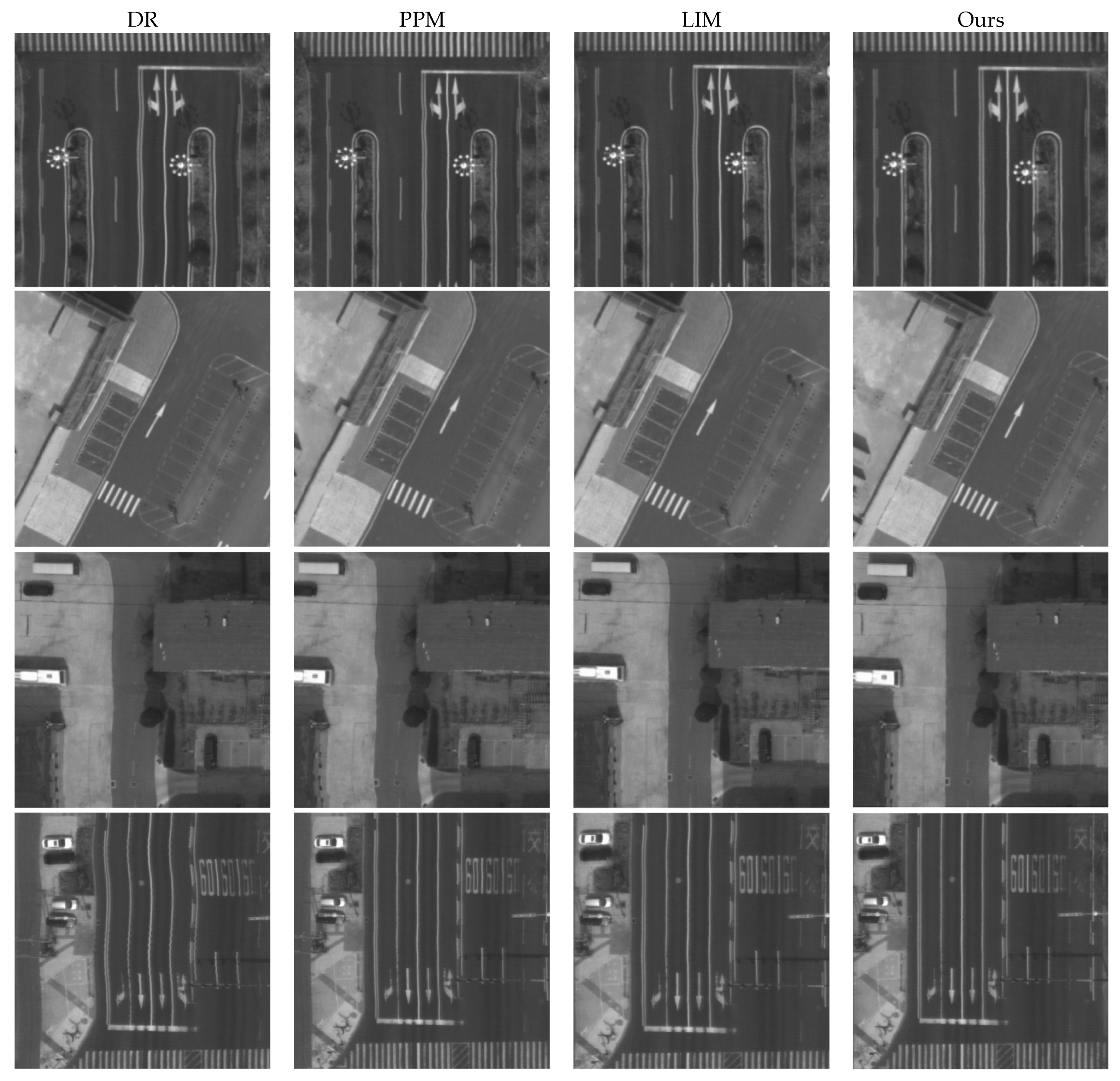
• We conducted comparative experiments with the LIM and PPM, demonstrating superior flexibility in the EOP refinement of airborne three-line scanners, resulting in improved visual outcomes and higher geometric processing accuracy.
• The proposed method was applied to the AMS-3000 data processing system, addressing the challenges faced by the AMS-3000 camera due to the low sampling rate and accuracy of its POS system, providing significant support for its product application.
• The remainder of this paper is organized as follows. Section 2 reviews related work on EOP refinement. Section 3 describes the characteristics of the AMS-3000 camera and the experimental data. Section 4 details the proposed method. Section 5 presents and discusses the experimental results. Section 6 concludes the study.

2. Related Work

Accurate EOP measurement during imaging is crucial for optimal georeferencing performance of high-resolution sensors. Current POS systems fail to provide the precise EOPs needed for three-line scanners to achieve optimal georeferencing accuracy because of their limited sampling frequency and measurement accuracy. Photogrammetrists strive to enhance EOP precision by analyzing factors that affect sensor stability and developing suitable refinement models. Tong et al. [30] summarized that jitter is a major factor impacting the EOP accuracy of both aerospace and aerial high-resolution imagery. To address this issue, some studies have employed high-performance attitude measurement devices to accurately measure platform vibrations and enhance positioning accuracy by compensating for jitter errors in EOPs [31,32,33]. Additionally, research using reliable attitude data has effectively balanced noise filtering and attitude approximation with penalized spline models [34,35]. However, these methods necessitate substantial financial and technical investments in sophisticated attitude measurement equipment.

In addition to direct measurement with equipment, EOPs can also be estimated and refined through algorithmic approaches. Currently, EOP refinement techniques primarily fall into two categories: posteriori compensation methods and self-compensation methods.

Posteriori compensation methods do not model the random jitter error and typically involve compensating for remaining errors in EOPs by analyzing residual patterns of control or tie points after the bundle adjustments. Teshima and Iwasaki [36] estimated a jitter frequency of approximately 1.5 Hz using tie point disparities between ASTER’s short-wave infrared sensors. Mattson et al. [37] addressed the jitter in HiRISE images through Fourier analysis, improving the EOPs by reducing the average amplitude of the jitter to less than one pixel. Tong et al. [38] detected a jitter of 0.67 Hz with an amplitude of 2.63 pixels in the ZY-3 three-line scanner using tie point disparities and compensated for it using a first-order Fourier series. Liu et al. [39] utilized high-resolution reference digital orthophoto map (DOM) and DEM to extract dense control points and modeled control point residuals with Fourier series, detecting a 0.65 Hz jitter in ZY-3. Although posteriori compensation methods effectively analyze the EOP error patterns, the EOP errors in airborne mapping systems differ significantly from those in spaceborne sensors. Airborne sensors’ EOP errors lack consistent periodicity and vary according to weather conditions, the coupled POS system, and the flight platform. Consequently, these variations make such methods unsuitable for the automated data processing systems of airborne mapping systems.

Compared to posteriori compensation methods, self-compensation methods are more efficient as they allow for the construction of various error description models and simultaneously yield precise orientation parameters and ground point coordinates. Bostelmann and Heipke [22] used the LIM to compensate for EOP errors in HRSC images, but improvements in more complex attitude jitters were not significant. Li et al. [25] employed a third-order PPM to mitigate EOP errors in HiRISE images, reducing checkpoint errors from 4.4 pixels to 0.29 pixels; however, the compensation was subject to time-varying drift errors. Thus, these two methods have limited application scenarios and do not adequately address the complexity and non-periodicity of EOP errors in airborne sensors. In contrast, the Gaussian Markov model offers greater flexibility in describing platform variations, but its application in aerial triangulation with three-line scanners and recovery methods for EOPs of scan lines without observations still requires further research [27,40]. McGlone [26] proposed a method where the orientation parameters of scan lines without observations can be obtained through linear interpolation after the bundle adjustment based on the Gaussian Markov model. However, this approach suffers approximation errors because it actually approximates a curve by a series of straight lines.

In summary, the Gaussian Markov model shows some potential in better describing the platform variations and better refining the EOPs for three-line scanner data. However, its effective application in aerial triangulation with three-line scanners and the recovery methods for the EOPs of unobserved scan lines still require further research.

3. Materials

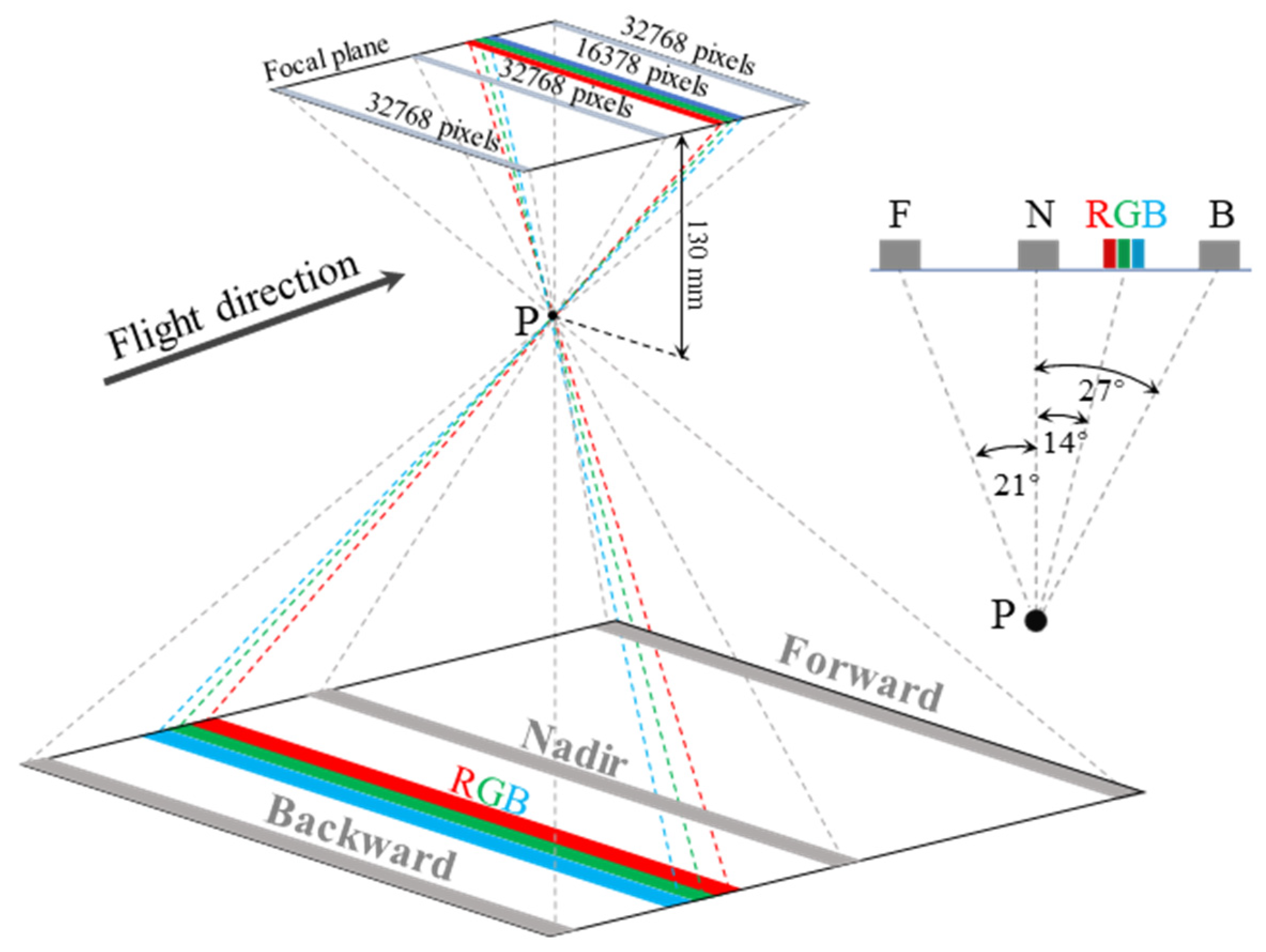
3.1. AMS-300 Mapping System

As depicted in Figure 1, the AMS-3000 is equipped with three panchromatic sensors, each containing 32,768 detectors, for capturing ground objects in forward, nadir, and backward views. In addition, it includes three color bands (red, green, and blue channels), each with 16,378 detectors, which facilitate both true and false color imaging. The nominal viewing angles of the forward, nadir, and backward CCD lines are 21, 0, and 27 degrees, respectively, achieving a base–height ratio of 0.89 to enhance stereo imaging accuracy.

The main parameters of the AMS-3000 are shown in

Table 1. Main parameters of the AMS-3000.

Item	Designed Parameter
Focal length (mm)	130
Radiometric resolution (bit)	16
Pixel size (μm)	Panchromatic: 5, RGB: 10
Spectrum (nm)	Panchromatic: 465–680, R: 608–662, G: 428–492, B: 428–492
Field of view (degree)	64
Weight (kg)	72.5

. The 16-bit radiometric resolution can provide rich details of the ground objects. Equipped with a 130 mm focal lens and 327,685 μm detectors, the AMS-3000 can capture swathes exceeding 2500 m in width with a resolution of 0.08 m at an altitude of 2000 m.

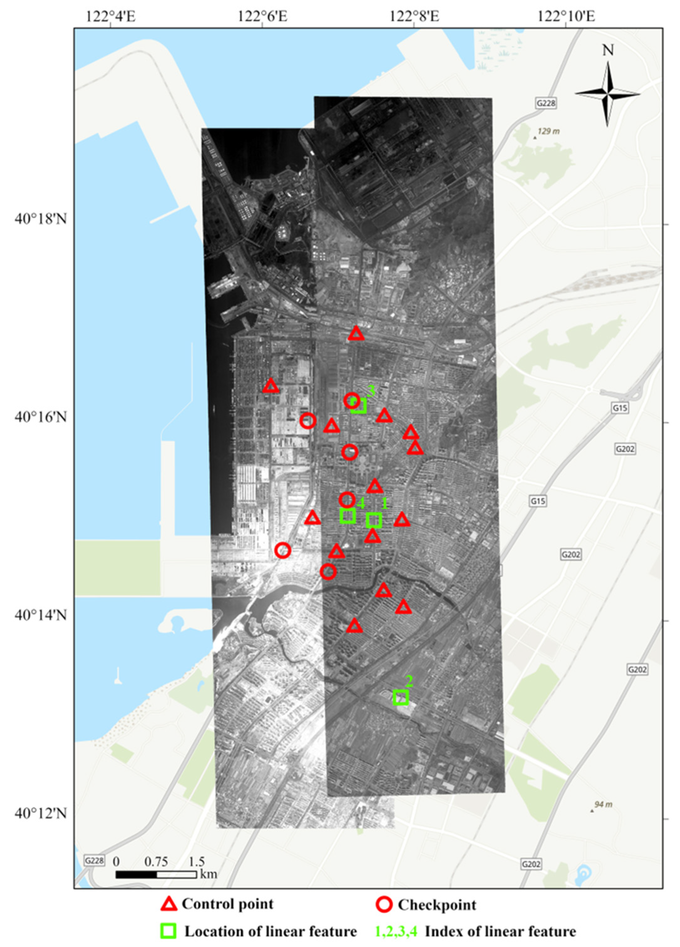
3.2. Experimental Data

Figure 2 displays the coverage of two image strips captured by the AMS-3000 used in this study. The data were collected by a Y-12 fixed-wing aircraft on 11 April 2022, at a flying altitude of 2600 m over the urban area of Bayuquan District, Yingkou City, Liaoning Province, China. The total coverage area spans approximately 73.7 square kilometers. These images showcase numerous buildings and roads and feature a ground resolution of 0.1 m. The Level 0 images of the left and right strips have row counts of 147,456 and 131,072, respectively.

We surveyed 20 control points to assess the geometric positioning accuracy after aerial triangulation, with 6 as checkpoints. Control points are marked with red triangles and checkpoints with red circles. The six checkpoints can validate the geometric accuracy of different methods [41]. Considering that checkpoints discretely distributed across an image spanning more than 130,000 lines are inadequate for assessing local EOP refinement performance, we manually measured linear features in four specified areas to evaluate the effectiveness of our method and others, as indicated by the yellow boxes in Figure 2.

3.3. EOP Problem Caused by the Self-Developed POS

The primary motivation for developing the AMS-3000 is its ability to meet the accuracy requirements of 1:1000 scale topographic mapping, and

Table 2. Chinese specifications for aerotriangulation of digital aerophotogrammetry (unit: meters).

Topographic Mapping Scale	Planar RMSE			Height RMSE
	Flat	Hills	Mountains	Flat	Hills	Mountains
1:1000	0.5	0.5	0.7	0.28	0.4	0.6
1:2000	1.0	1.0	1.4	0.28	0.4	1.0

displays some of the Chinese specifications for aerotriangulation of digital aerophotogrammetry [42]. Considering Canadian manufacturer Applanix’s leadership in aided inertial systems [6], the AMS-3000 was initially equipped with their POS AV610 inertial navigation system, with GNSS and IMU sampling frequencies of 200 Hz and 1000 Hz, respectively. Despite Shannon’s theorem requiring an IMU frequency of at least 2000 Hz for precise attitude recovery at 1000 Hz imaging frequency, the strict photogrammetric flight plan and POS Pac 8 processing software ensured that the provided EOPs were reliable. Previous work with the AMS-3000 conducted the bundle adjustment using the LIM on the 0.1 m resolution Yangjiang city dataset and achieved accuracies of 0.088 m, 0.092 m, and 0.176 m in the X, Y, and Z directions, respectively [4,42]. The results indicated that the georeferencing accuracy of the AMS-3000 coupled with the POS AV610 can meet the accuracy demands of 1:1000 scale topographic mapping.

However, due to hardware issues with the POS AV610, the AMS-3000 was subsequently equipped with a self-developed POS product for later missions, with the GNSS and IMU sampling frequencies reduced to 2 Hz and 200 Hz, respectively—far below the requirements suggested by Shannon’s theorem. The main parameters of the POS AV610 and the self-developed POS product are shown in

Table 3. Main parameters of the POS AV610 and the self-developed POS product.

Performance	POS AV610	Self-Developed POS Product
Position (m)	Horizontal: 0.05, vertical: 0.1	Horizontal: 0.05, vertical: 0.1
Velocity (m/s)	0.005	0.02
Roll and pitch (degree)	0.0025	0.015
True heading (degree)	0.005	0.030
GNSS frequency (Hz)	200	2
IMU frequency (Hz)	1000	200
Post-processing software	POS Pac 8	self-developed software

. The roll and pitch accuracy of the self-developed POS product is 0.015 degrees, and the heading accuracy is 0.03 degrees, both of which are six times worse than that of the POS AV 610. Considering the 130 mm focal length and 5 μm detector of AMS-3000, the 0.015-degree performance in roll angle would cause up to a 6.8-pixel error.

To demonstrate the EOP issues associated with the self-developed POS, we performed a visual georeferencing performance comparison by projecting Level 0 images onto a mean elevation plane using EOPs provided by two different POS systems. The dataset using the POS AV610 was collected on 29 May 2020, covering the Yushu area in Jilin Province, China, while the dataset using the self-developed POS was the experimental data described in Section 3.2.

As shown in Figure 3, the Level 0 images suffer severe distortion caused by the motion of the sensor along with jitter. Comparing the Level 1 images, it is evident that the direct georeferencing results based on the POS AV610 are significantly better than those based on the self-developed POS in terms of recovering the shape of ground objects. The self-developed POS failed to provide accurate EOPs to recover the shape of the same ground objects observed at three different times. Impacted by the visible waveform distortions that have a cycle of about 150 lines and continuously changing amplitude, the AMS-3000 loses the ability to support stereoscopic vision.

Thus, this study aims to rectify these waveform distortions to an acceptable level by refining the EOPs provided by the self-developed POS, enabling the AMS-3000 to produce 1:1000 scale topographic maps that meet the Chinese specifications.

4. Method

This study introduces a method to correct for image distortions in the three-line scanner caused by inaccurate EOPs delivered by POS system on aerial platform. The core idea of this approach involves utilizing a first-order Gaussian Markov process to develop a more accurate model of the orientation parameters, followed by cubic spline interpolation to obtain EOPs of all lines, thereby providing precise EOP error compensation. As illustrated in Figure 4, the overall technical process can be divided into four key modules based on AMS-3000 data:

• Level 1 image generation: This step addresses severe distortions in the original images, setting the stage for further processing.
• Tie point matching: This involves obtaining tie points across images from different views to collect extensive observations critical for the bundle adjustment.
• Bundle adjustment: Utilizing the Gaussian Markov model, this stage accurately models the motion of the sensor and is incorporated into the bundle adjustment process.
• Cubic spline interpolation: Applying cubic spline interpolation, EOPs of lines without observations are obtained.

4.1. Modeling the Sensor Motion with the First-Order Gauss-Markov Model

Aerial photogrammetry requires that the aircraft flies at a stable speed and attitude to ensure that the nadir view is perpendicular to the ground and that there are no gaps in the images. However, the atmospheric turbulence and the engine operation may cause random changes in attitude and position, which are generally processed as white noise [43]. The simplified physical model describing sensor motion can be represented by Equation (1):

$$\left[\begin{array}{c}\begin{array}{c}{X}_{t+1}\\ Y_{t+1}\\ Z_{t+1}\end{array}\\ {\omega }_{t+1}\\ {\phi }_{t+1}\\ {\kappa }_{t+1}\end{array}\right]=\left[\begin{array}{c}\begin{array}{c}{X}_t\\ Y_t\\ Z_t\end{array}\\ {\omega }_t\\ {\phi }_t\\ {\kappa }_t\end{array}\right]+\Delta t\left[\begin{array}{c}\begin{array}{c}{V}_{X,t+1}\\ V_{Y,t+1}\\ V_{Z,t+1}\end{array}\\ {\mathsf{\Omega }}_{X,t+1}\\ {\mathsf{\Omega }}_{Y,t+1}\\ {\mathsf{\Omega }}_{Z,t+1}\end{array}\right]+\Delta t\left[\begin{array}{c}\begin{array}{c}{Vw}_{X,t+1}\\ V{w}_{Y,t+1}\\ V{w}_{Z,t+1}\end{array}\\ \mathsf{\Omega }{w}_{X,t+1}\\ {\mathsf{\Omega }w}_{Y,t+1}\\ \mathsf{\Omega }{w}_{Z,t+1}\end{array}\right]$$

(1)

where $X_t,Y_t$, and $Z_t$ represent the three positional parameters at time $t$; ${\omega }_t,{\phi }_t$ and ${\kappa }_t$ are the three attitude parameters at time $t$; $V_{X,t+1},V_{Y,t+1}$ and $V_{Z,t+1}$ represent the velocities along the X, Y, and Z axes at time $t+1$, respectively; ${\mathsf{\Omega }}_{X,t+1},{\mathsf{\Omega }}_{Y,t+1}$ and ${\mathsf{\Omega }}_{Z,t+1}$ represent the angular velocities along the X, Y, and Z axes at time $t+1$, respectively; ${Vw}_{X,t+1},V{w}_{Y,t+1}$ and $V{w}_{Z,t+1}$ represent the velocity noise caused by the environments along the X, Y, and Z axes at time $t+1$, respectively; $\mathsf{\Omega }{w}_{X,t+1},{\mathsf{\Omega }w}_{Y,t+1}$ and $\mathsf{\Omega }{w}_{Z,t+1}$ represent the angular velocity noise along the X, Y, and Z axes at time $t+1$, respectively; $\Delta t$ is the imaging time interval.

Equation (1) demonstrates that the exterior orientation elements at each moment are closely related to those of the previous moment. Common methods typically utilize PPM or LIM to describe the EOPs, assuming that EOPs can be expressed with smooth curves over a certain time period. However, when the POS system cannot provide accurate EOPs filtered of noise, using smooth curves to model these elements is inappropriate. This is because they fail to account for random noise and lack the capability to estimate this noise during the bundle adjustment process.

To more precisely describe and compensate for EOP errors, a first-order Gaussian Markov model is employed. This model incorporates a noise observation for each exposure, assuming strong correlations between consecutive exposures to enhance flexibility and closely mimic real attitude dynamics. The model’s continuity and the relationships between states are governed by the first derivatives, as detailed in Equation (2):

$$\frac{dx}{dt}+{\beta }_1\left(t\right)x=w(t)$$

(2)

where $x$ represents the random variable and $t$ denotes the time; ${\beta }_1\left(t\right)$ is a time-dependent function that becomes constant if the process is assumed to be stationary; $w(t)$ represents random noise with zero mean and arbitrary variance.

We treat the orientation parameters at each exposure as samples from a continuous Gaussian Markov process, resulting in the discrete form presented in Equation (3):

$$\frac{x_i-x_{i-1}}{∆t}+{\beta }_1\left(t_i\right)x_{i-1}=w(t_i)$$

(3)

where $x_i$ represents the orientation parameters at time $i$; $∆t$ is the time interval.

Thus, orientation parameters at time $i$ can be expressed by those at time $i-1$, as shown in Equation (4):

$$\begin{array}{cc}{x}_i& =\left(1-∆t·{\beta }_1\left(t_i\right)\right)x_{i-1}+∆t·w\left(t_i\right)\hfill \\ \hspace{1em}& =\left(1-s\right)x_{i-1}+n_i\hfill \end{array}$$

(4)

where $n_i$ represents a Gaussian noise term with a mean of zero. Assuming a stationary process, $s=∆t·{\beta }_1\left(t_i\right)$ serves as a constant that quantifies the correlation strength, with $s\ll 1$. The constant $s$ can be adjusted based on practical conditions to determine how long after the current moment the error’s influence becomes negligible.

Finally, the errors in the EOPs at each exposure moment are established with a Gaussian Markov model, as illustrated in Equation (5):

$$\begin{gathered} {∆X}_i=\left(1-s\right){∆X}_{i-1}+n_{X,i} \\ {∆Y}_i=\left(1-s\right){∆Y}_{i-1}+n_{Y,i} \\ {∆Z}_i=\left(1-s\right){∆Z}_{i-1}+n_{Z,i} \\ {∆\omega }_i=\left(1-s\right){∆\omega }_{i-1}+n_{\omega ,i} \\ {∆\phi }_i=\left(1-s\right){∆\phi }_{i-1}+n_{\phi ,i} \\ {∆\kappa }_i=\left(1-s\right){∆\kappa }_{i-1}+n_{\kappa ,i} \end{gathered}$$

(5)

where ${∆X}_i,{∆Y}_i$ and ${∆Z}_i$ represent the positional errors at time $i$; ${∆\omega }_i,{∆\phi }_i$ and ${∆\kappa }_i$ are the attitude errors at time $i$; $n_{X,i},n_{Y,i},n_{Z,i},n_{\omega ,i},n_{\phi ,i}$ and $n_{\kappa ,i}$ represent the zero-mean noise terms associated with the EOPs at time $i$.

Only scan lines that contain image point observations are needed for the bundle adjustment. Considering the zero-mean assumption of the noise terms, EOP errors between observed lines can be expressed by Equation (6):

$$\begin{gathered} {∆X}_i={\left(1-s\right)}^m{∆X}_{i-m}+n_{X,i} \\ {∆Y}_i={\left(1-s\right)}^m{∆Y}_{i-m}+n_{Y,i} \\ {∆Z}_i={\left(1-s\right)}^m{∆Z}_{i-m}+n_{Z,i} \\ {∆\omega }_i={\left(1-s\right)}^m{∆\omega }_{i-m}+n_{\omega ,i} \\ {∆\phi }_i={\left(1-s\right)}^m{∆\phi }_{i-m}+n_{\phi ,i} \\ {∆\kappa }_i={\left(1-s\right)}^m{∆\kappa }_{i-m}+n_{\kappa ,i} \end{gathered}$$

(6)

Since $n_{X,i},n_{Y,i},n_{Z,i},n_{\omega ,i},n_{\phi ,i}$ and $n_{\kappa ,i}$ are considered as fictitious observations assigned an a priori value of zero, for a control point observed on three image lines, the number of unknown EOP errors is reduced from 18 to 6. Similarly, for a tie point observed on three lines, the number is reduced from 21 to 9. Thus, this approach allows for significant savings in computational effort and can prevent over-parameterization.

4.2. EOP Refinement Workflow

4.2.1. Level 1 Image Generation

As illustrated in Figure 3, the correspondences on Level 0 tri-view images of AMS-3000 exhibit different shape deformations due to varying jitter impacts. These deformations severely limit the number and accuracy of matching points and may cause the subsequent bundle adjustment to diverge.

To resolve this, Level 0 images are rectified to Level 1 images using EOPs provided by the self-developed POS system. Despite the POS system’s unideal measurement performance, post-processing software still managed to recover the motion of the sensor to a certain extent for correcting jitter distortions. The remaining distortions, which can be seen as the result of minor local rotations, have negligible effects on matching methods robust to rotation and scale, such as SIFT [44].

It is critical to note that Level 1 images are used exclusively for feature point matching. Once matched, these points are reprojected onto the original Level 0 images for further bundle adjustment processing. The local affine transformation method is employed to obtain each point location on the Level 0 image, which once emerged in the pseudo-code provided by the Leica Geosystems software 2.2 development kit [45].

4.2.2. Tie Point Matching

The key to the bundle adjustment is minimizing the reprojection error of all tie points. Therefore, ensuring the precision and adequacy of tie points is crucial for EOP refinement without relying on reference data. This paper only uses the tri-view panchromatic images for matching and strictly selects tie points with overlaps of three degrees or more for the bundle adjustment. The implementation process is as follows: First, Level 1 tri-view images undergo Wallis filtering to eliminate radiometric differences between images. Next, dense matching is performed between the nadir Level 1 images and the forward Level 1 images to obtain points with double observations. These doubly observed points are then projected onto the backward Level 1 image using geographic coordinates, obtaining seed points. Local refinement matching is conducted around the seed points to precisely locate the tie points on the backward images. For adjacent strip images, tie points are first matched on the nadir Level 1 images, then similarly projected onto the forward and backward images of each strip using geographic coordinates as seed points, where refined matching yields points with sixfold observations.

During the dense matching process, we employ the two-step expansion dense matching algorithm proposed by Zhang et al. [46]. This algorithm, robust to rotation and scale, requires no prior information and can generate dense matching points on linear array images. The matching window size is adjustable, allowing for a variable number of matching points to be obtained as needed.

To compensate for the waveform distortion, which has a cycle of about 150 lines as shown in Figure 3b, observations with an interval of at least 37 lines are required. In our case, at least 50 tie points are matched within a 37-line interval to provide redundant observations.

4.2.3. Bundle Adjustment

The first step in performing bundle adjustment is establishing the observation equation. The initial observation equation is provided by establishing the relationship between the object coordinates of ground points and their corresponding image coordinates, as shown in Equation (7):

$$\left[\begin{array}{c}X\\ Y\\ Z\end{array}\right]=\left[\begin{array}{c}{X}_S\\ Y_S\\ Z_S\end{array}\right]+\lambda R\left[\begin{array}{c}x-x_0\\ y-y_0\\ -f\end{array}\right]$$

(7)

where $(x,y)$ are the image coordinates of a ground point; $(x_0,y_0)$ are the coordinates of the principal point; $R$ is the rotation matrix defined by the three attitude parameters; $(X,Y,Z)$ are the ground point coordinates; $(X_S,Y_S,Z_S)$ are the coordinates of the perspective center in the object space coordinate system; $f$ is the focal length of the camera; and $\lambda$ is the scale factor.

The bundle adjustment optimizes the EOPs by minimizing the reprojection error observed for each image point. By integrating Equation (6), which defines the stochastic behavior of EOPs, with Equation (7), which establishes the geometric relationship of the points, we derive the observational model for aerial triangulation, as shown in Equation (8):

$$\begin{array}{cc}\hfill v_c& =A{x}_{eo}+B{x}_g-l_c; P_C\hfill \\ \hfill v_g& ={Ex}_g-l_g; P_g\hfill \\ \hfill v_{eo}& \hfill =E{x}_{eo,i}-{Cx}_{eo,i-1}; P_{eo}\end{array}$$

(8)

where $x_{eo}$ is the vector of unknown corrections for EOPs; $x_g$ is the ground coordinates vector; $A$, $B$, $C$, and $E$ are the corresponding design matrices; $l_c$ and $l_g$ are discrepancy vector; and $P_C$, $P_g$, and $P_{eo}$ are weight matrices.

4.2.4. Cubic Spline Interpolation

The first-order Gaussian Markov model does not perform smoothing or interpolation of exterior orientation elements during the bundle adjustment, unlike PPM or LIM. This approach increases the model’s flexibility but the EOPs of lines without observations are not modeled with a smooth curve. To address this, after completing the bundle adjustment, it is necessary to apply interpolation to derive the EOPs for scan lines without observations. In this paper, spline regression is used to process the bundle adjustment results, specifically employing cubic splines when the order is three [47,48].

Let $x$ denote the row number, and the essential idea of the cubic spline interpolation is to fit a piecewise function of the form in Equation (9):

$$S\left(x\right)=\left\{\begin{array}{cc}{s}_1(x)& x\in [x_1,x_2]\\ s_2(x)& x\in [x_2,x_3]\\ ⋮& ⋮\\ s_n(x)& x\in [x_{n-1},x_n]\end{array}\right.$$

(9)

where $n$ is the number of the numerical data to fit and $s_i$ is a third-degree polynomial defined by Equation (10):

$$s_i\left(x\right)=a_i{(x-x_i)}^3+b_i{(x-x_i)}^2+c_i\left(x-x_i\right)+d_i$$

(10)

where $i=\mathrm{1,2},\cdots ,n-1$, $a_i,b_i,c_i$ and $d_i$ are the spline coefficients.

For each $s_i\left(x\right)$, the first and second derivatives are defined as Equation (11):

$$\begin{array}{cc}\hfill s_i^{\prime }\left(x\right)& ={3a}_i{\left(x-x_i\right)}^2+{2b}_i\left(x-x_i\right)+c_i\hfill \\ \hfill s_i^{″}(x)& ={6a}_i{(x-x_i)}^2+{2b}_i\hfill \end{array}$$

(11)

where $i=\mathrm{1,2},\cdots ,n-1.$

To estimate the coefficients, the cubic spline must conform to the following conditions:

1. the piecewise function $S\left(x\right)$ interpolates all points.

2. $S\left(x\right)$ is twice continuously differentiable on $[x_1,x_n]$.

Let ${\delta }_i=x_{i+1}-x_i$ and impose these conditions on n points, and we can obtain Equation (12):

$$\begin{array}{cc}\hfill a_i{{\delta }_i}^3+b_i{{\delta }_i}^2+c_i{\delta }_i+d_i& =y_{i+1}\hfill \\ \hfill {3a}_i{{\delta }_i}^2+{2b}_i{\delta }_i+c_i-c_{i+1}& =0\hfill \\ \hfill {6a}_i{{\delta }_i}^2+{2b}_i-{2b}_{i+1}& =0\hfill \\ \hfill d_i& =y_i\hfill \end{array}$$

(12)

where $y$ denotes the orientation parameters.

If we let ${\eta }_i=s_i^{″}\left(x\right)={2b}_i$ and perform several substitution steps in Equation (12), we can obtain Equation (13):

$${\delta }_i{\eta }_i+2\left({\delta }_i+{\delta }_{i+1}\right){\eta }_{i+1}+{\delta }_{i+1}{\eta }_{i+2}=6(\frac{y_{i+2}-y_{i+1}}{{\delta }_{i+1}}-\frac{y_{i+1}-y_i}{{\delta }_i})$$

(13)

According to Equation (13), we can establish $n-2$ equations based on the points. To solve for the $n$ unknowns ${\eta }_i(i=\mathrm{1,2},\cdots ,n)$ in Equation (13), two other conditions must be imposed. Generally, several end conditions are employed to determine the unique cubic spline, such as the natural end condition, clamped end condition, and not-a-knot end condition [47]. In this paper, we use the natural end condition, which requires the second derivatives of the spline being zero at the ends $x_1$ and $x_n$. After obtaining ${\eta }_i(i=\mathrm{1,2},\cdots ,n)$, the coefficients of the cubic spline can be determined by Equation (12).

5. Results and Discussion

5.1. Experimental Settings

To evaluate the performance of our method, we conducted a comparative analysis of the proposed method with three other methods: the direct rectification method (DR), PPM [25], and LIM [22]. DR uses EOPs provided by POS to directly derive 3D coordinates for tie points and perform rectification without the bundle adjustment, which can be used as a reference for evaluating improvement. In the experiments, both PPM and LIM used third order and were set to intervals of 50 rows. All models used the same control points and tie points without additional constraints like linear features.

Given that checkpoints do not adequately demonstrate the effectiveness of EOP refinement by the three methods, a quantitative assessment was conducted by manually measuring four linear features on the Level 1 nadir images, the positions of which are delineated by the rectangular boxes in Figure 2. To ensure a consistent basis for evaluating the EOP refinement performance of the three methods, the sample points on these linear features were projected onto the Level 0 images (as depicted in Figure 5). During measurement, the number and spacing of sample points should be sufficient to reflect the trend of waveform distortions. Due to the differing frequencies and amplitudes of waveform distortions on the four lines, the performance of the three methods on each line needs to be compared individually. Therefore, the number of sampling points on the four lines does not need to be consistent. Along these lines, sample points were manually collected, yielding totals of 35, 57, 37, and 73 points, respectively.

5.2. Overall Comparison

5.2.1. Quantitative Evaluation

Table 4. Geo-referencing accuracy at checkpoints (unit: meters).

Method	X		Y		Z
	Std	RMSE	Std	RMSE	Std	RMSE
DR	3.943	4.040	3.835	3.947	0.587	6.007
PPM	0.102	0.115	0.079	0.089	0.200	0.208
LIM	0.097	0.112	0.074	0.083	0.198	0.205
Ours	0.076	0.088	0.069	0.078	0.145	0.150

Note: The best results are highlighted in bold.

presents the standard deviations (std) of checkpoint residuals and the root mean square errors (RMSE) for both DR and the three bundle adjustment methods. The standard deviation of checkpoint residuals and RMSE are defined by Equation (14):

$$std=\sqrt{\frac{{\sum }_i^n{(r_i-\overline{r})}^2}{n-1}}, RMSE=\sqrt{\frac{{\sum }_i^n{(x_i-{\widehat{x}}_i)}^2}{n}}$$

(14)

where $r_i$ is the residual error of the $i$ checkpoint; $\overline{r}$ is the mean value of the checkpoint residual errors; $x_i$ is the ground coordinates of the $i$ checkpoint using the space intersection; ${\widehat{x}}_i$ is the true ground coordinates of the $i$ checkpoint; $n$ is the number of checkpoints.

The standard deviations of checkpoint residuals and the RMSE can indicate the concentration and the absolute accuracy of the results, respectively. By directly using the EOPs provided by the POS, the geometric accuracies determined by DR along the X, Y, and Z axes were 4.04 m, 3.947 m, and 6.007 m, respectively. The standard deviation of residuals in the X-direction exceeded that in the Y-direction by 0.108 m, which corresponded to more than one pixel. This variation can be attributed to a more significant roll angle jitter, which predominantly impacts accuracy in the X-direction [43,49]. This discrepancy may also be influenced by the rigorous control over pitch and yaw angles by the flight platform to prevent image fractures.

Following the implementation of the three comparison methods, there was a noticeable enhancement in both the standard deviations of residuals and the RMSEs across all three axes. Notably, the LIM achieved geometric positioning accuracies of 0.112 m, 0.083 m, and 0.205 m in the X, Y, and Z directions, respectively, slightly exceeding the performance of the PPM by 0.003 m, 0.006 m, and 0.003 m in these respective directions. Our method demonstrated RMSE of 0.088 m, 0.078 m, and 0.15 m in the X, Y, and Z axes, respectively, which are better than the PPM by 0.027 m, 0.011 m, and 0.058 m, and better than the LIM by 0.024 m, 0.005 m, and 0.055 m. Furthermore, our method’s residual standard deviation along the X-axis was 0.076 m, indicating a high degree of reliability in geometric positioning along this axis. However, these insignificant improvements, as evaluated by checkpoints discretely distributed across the long strip images, cannot effectively demonstrate the local compensation performance for waveform distortions.

Further analysis was performed on the fitting accuracy of four linear features across different flight strip areas, as shown in

Table 5. EOP refinement performance (unit: pixels).

Method	Line 1			Line 2			Line 3			Line 4
	Max	Min	RMSE	Max	Min	RMSE	Max	Min	RMSE	Max	Min	RMSE
DR	1.55	0.01	0.85	2.36	0.00	1.01	2.68	0.03	1.24	2.87	0.02	1.50
PPM	0.7	0.01	0.31	2.00	0.02	0.91	3.86	0.07	1.55	1.7	0.01	0.71
LIM	1.23	0.01	0.54	1.18	0.01	0.51	1.59	0.02	0.67	1.78	0.01	0.65
Ours	0.65	0.01	0.27	0.71	0.00	0.28	1.02	0.00	0.47	0.93	0.01	0.36

Note: The best results are highlighted in bold.

. The results indicate that the DR method achieved fitting accuracies of 0.85 pixels, 1.01 pixels, 1.24 pixels, and 1.5 pixels for lines 1, 2, 3, and 4, respectively. Notably, lines 1 and 4, located in the middle of the strip, and lines 2 and 3, at the ends, showed that EOP errors did not exhibit a straightforward linear trend.

After the bundle adjustment, all three methods can refine the EOPs provided by the POS, but their effectiveness varies. Our method demonstrated the highest refinement performance across all approaches, achieving fitting accuracies of 0.27 pixels, 0.28 pixels, 0.47 pixels, and 0.36 pixels on the four lines. It outperformed the LIM by 50%, 45.1%, 29.9%, and 44.6%, and the PPM by 12.9%, 69.2%, 69.6%, and 49.3%.

Compared to the PPM, our method demonstrates a more stable performance. The PPM showed variable effectiveness, with sub-pixel accuracies on lines 1, 2, and 4 at 0.31 pixels, 0.91 pixels, and 0.71 pixels, respectively, but markedly underperformed on line 3 with an accuracy of 1.55 pixels—exceeding DR’s 1.24 pixels. The inconsistency in PPM’s results primarily stems from its fixed segment intervals, which lack the flexibility to adapt to the stochastic nature of jitter, leading to suboptimal polynomial fitting.

Moreover, our method more accurately characterizes sensor jitter compared to the LIM. Although the third-order LIM achieved accuracies of 0.54 pixels, 0.51 pixels, 0.67 pixels, and 0.65 pixels, achieving pixel-level precision, its design constrained by four orientation fixes restricts its ability to model stochastic jitter dynamically. This limitation impacts its overall compensation accuracy, which our Gaussian Markov model approach effectively addresses, offering a more adaptable and precise solution for jitter compensation.

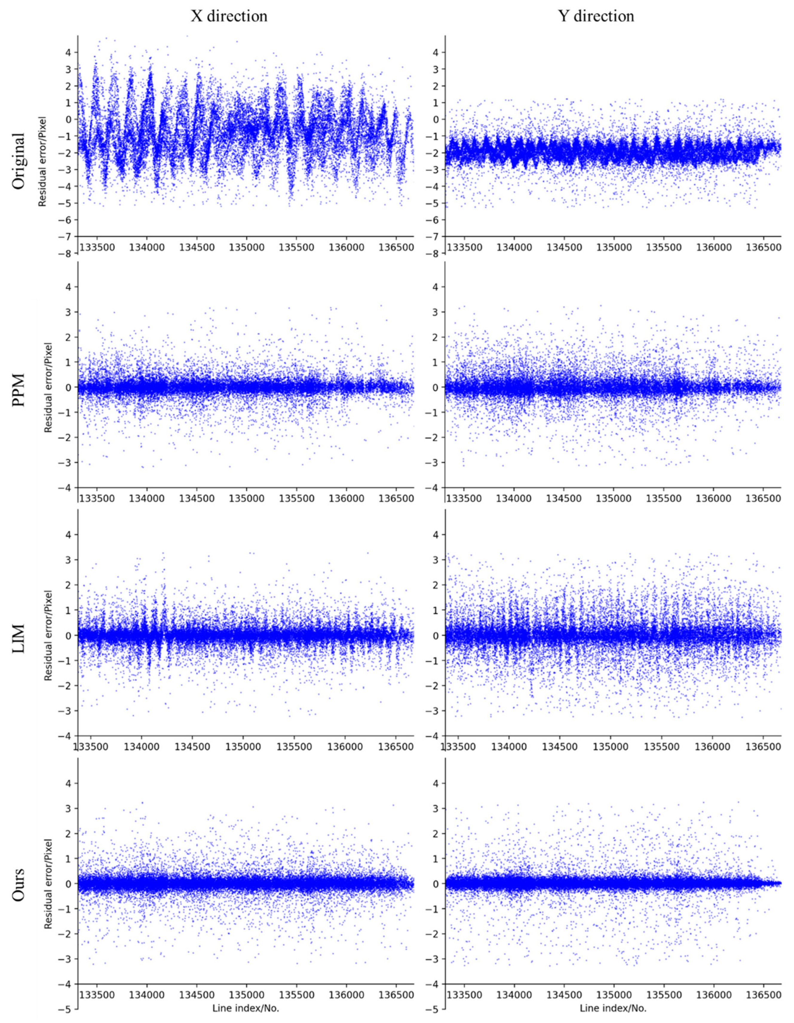
5.2.2. Comparison of Residual Distributions at Tie Points

Figure 6 depicts a comparison of residual distributions at tie points, encompassing approximately 3000 scan lines around Line 1. From the first row to the last row, the figure shows the results of the original EOPs, PPM, LIM, and our method, respectively. The original EOPs, provided by the self-developed POS, resulted in waveform distortions at about 6 Hz frequency in both the X and Y directions. The amplitude of the waveform distortion in the X direction is about 3 pixels, significantly worse than the 1-pixel amplitude in the Y direction. The residual distribution in both directions deviates from zero due to the offset between the GNSS antenna and the projection center and the misalignment between the IMU and the sensor.

All three methods reduced the waveform distortion around Line 1 to within one pixel and also compensated for the offset and misalignment errors. However, our method exhibited the most concentrated residual distributions and did not show any waveform distortion, unlike the LIM. The third-order LIM, limited by its four orientation fixes, reduces its ability to model EOPs affected by jitter errors with varying frequency and amplitude. On the other hand, the PPM showed a more concentrated pattern than the LIM, indicating that it better handles jitter errors around the Line 1 area.

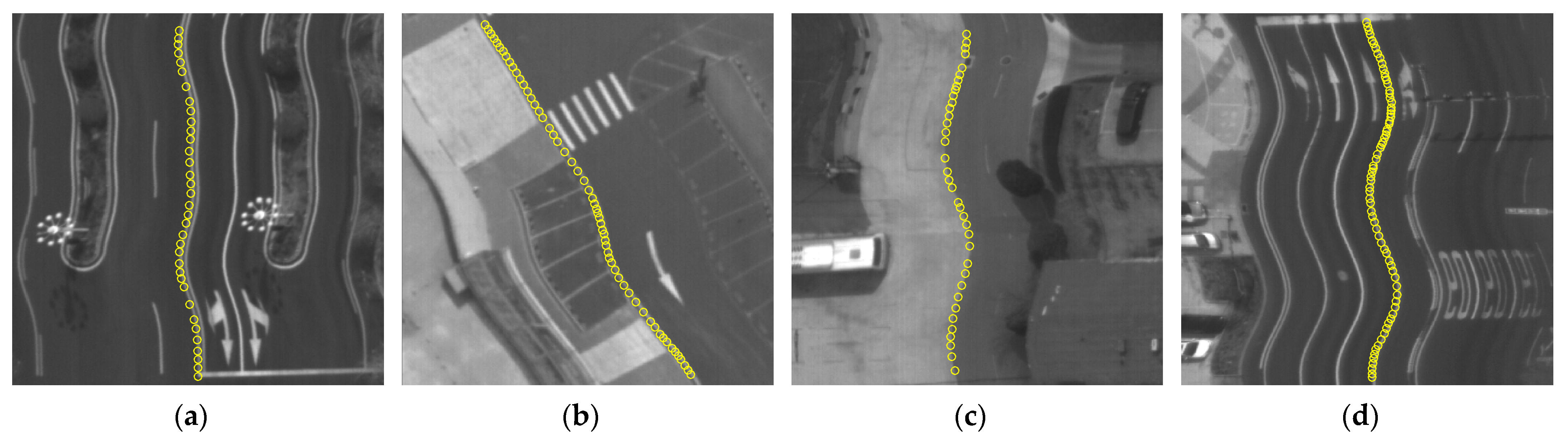
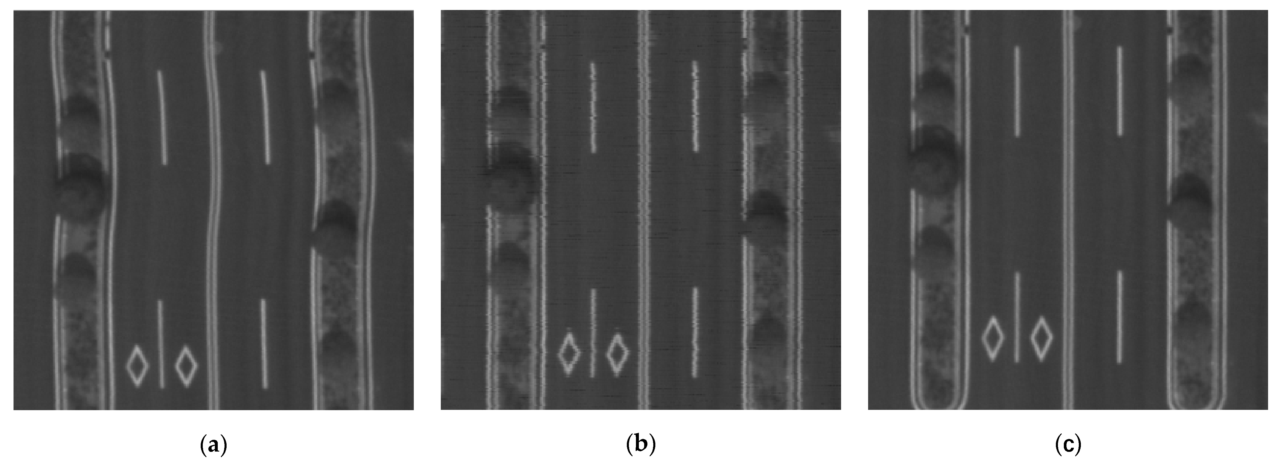
5.2.3. Visual Performance of EOP Refinement

To more vividly demonstrate the superiority of our method in compensating for EOP errors, Figure 7 compares the rectification results of the proposed method with the three comparative methods across four lines. It is evident from Figure 7 that the DR method led to significant waveform distortions, with varying degrees and frequencies of distortion along each line. Notably, Line 4 exhibited high-frequency distortions, indicating that the flight platform experienced complex jitter interference beyond the measurement capabilities of the self-developed POS system. For the high-frequency distortions observed particularly on Line 4, all three comparative methods effectively compensated through smoothing techniques.

Our method consistently outperformed the PPM and LIM in compensating for jitter across all four lines, avoiding issues such as the negative optimization observed with PPM on Line 3. While minor distortions are still visible in the visual results from our method in Figure 7, these primarily stem from the inherent limitations of relying solely on tie points for jitter compensation. The accuracy of tie point matching can impact the final results, and the bundle adjustment process can only reduce errors to an acceptable level, not eliminate them entirely. As quantified in Table 5, these visually perceptible distortions are controlled within 0.5 pixels. For an AMS-3000 dataset with a 0.1 m resolution, positioning errors due to these distortions are kept below 0.05 m, meeting the 1:1000 scale topographic mapping specifications in Table 2, which is acceptable.

5.3. Effectiveness of Cubic Spline Interpolation

The bundle adjustment improves the EOPs of those lines with observations, but it is also important to recover the EOPs of lines without observations to ensure image quality. Our method particularly emphasizes the importance of cubic spline interpolation for obtaining EOPs of unobserved lines. Since the proposed method is established based on Equation (6), we obtained a comparison group of EOPs by following Equation (6) and set the noise term as zero to compare with the group of EOPs based on cubic spline interpolation. The rectified nadir Level 1 images based on the original, the comparison, and the cubic spline interpolation processed EOPs are shown in Figure 8.

As shown in Figure 8a, distortions in the X direction are distinctly visible using original EOPs for image rectification. After the bundle adjustment, as shown in Figure 8b,c, these waveform distortions with a cycle of about 150 lines are visibly eliminated, confirming that the jitter errors have been compensated. However, Figure 8b demonstrates that the comparison EOP group leads to many jagged edges on Level 1 images. The main reason is that it is too rigid to directly obtain EOPs of lines without observations by assuming the noise term as zero. In contrast, cubic spline can obtain smooth results. Moreover, the constraint of cubic spline crossing all points makes sure that the interpolation process would not change the bundle adjustment result. Therefore, integrating cubic spline interpolation with the Gaussian Markov model effectively refines the EOPs by compensating for jitter errors beyond the measurement ability of the self-developed POS system, restoring the true shape of ground targets.

6. Conclusions

In this paper, a novel Gaussian Markov EOP refinement method enhanced by cubic spline interpolation is introduced to improve inaccurate EOPs provided by an unideal POS system. The method involves projecting tri-view images onto a mean elevation plane using initial EOPs to generate Level 1 images for dense tie point matching. Matched points are back-projected to the original Level 0 images as observations, followed by a bundle adjustment based on the Gaussian Markov modeled EOPs, with cubic spline interpolation applied to ensure image quality.

Based on the EOP challenge brought by the self-developed POS on the first Chinese airborne mapping system AMS-3000 with 1000 HZ imaging frequency, comparative assessments with the PPM and LIM revealed our method enhances geo-referencing accuracy, EOP refinement performance, and visual performance. Specifically, our method achieved geo-referencing accuracies of 0.088 m, 0.078 m, and 0.150 m in the X, Y, and Z directions, respectively. It also attained EOP refinement accuracies of 0.27 pixels, 0.28 pixels, 0.47 pixels, and 0.36 pixels on four lines, marking improvements over the LIM by 50%, 45.1%, 29.9%, and 44.6%, and over the PPM by 12.9%, 69.2%, 69.6%, and 49.3%. These results underscore the effectiveness of integrating Gaussian Markov modeling with cubic spline interpolation in addressing complex EOP errors.

However, since the AMS-3000 is currently focused on collecting urban area data, the experimental results only demonstrate that the proposed method allows the AMS-3000 to meet the Chinese specifications for 1:1000 scale topographic mapping in flat areas. Therefore, the reliability of our method will still need further evaluation if datasets covering hills and mountains are collected by the AMS-3000 in the future.

References

1. Gruen, A.; Zhang, L.; Wang, X. 3D City Modeling with TLS (Three Line Scanner) Data. Int. Arch. Photogramm. Remote Sens. Spat. Inf. Sci. 2003, 34, 24–27. [Google Scholar]
2. Müller, J.; Gärtner-Roer, I.; Thee, P.; Ginzler, C. Accuracy Assessment of Airborne Photogrammetrically Derived High-Resolution Digital Elevation Models in a High Mountain Environment. ISPRS J. Photogramm. Remote Sens. 2014, 98, 58–69. [Google Scholar] [CrossRef]
3. Zhu, X.; Pang, G.; Chen, P.; Tao, Y.; Zhang, Y.; Zuo, X. Research on Urban Construction Land Change Detection Method Based on Dense DSM and TDOM of Aerial Images. Int. Arch. Photogramm. Remote Sens. Spat. Inf. Sci. 2020, 42, 205–210. [Google Scholar] [CrossRef]
4. Xi, K.; Duan, Y. AMS-3000 Large Field View Aerial Mapping System: Basic Principles and the Workflow. Int. Arch. Photogramm. Remote Sens. Spat. Inf. Sci. 2020, 43, 79–84. [Google Scholar] [CrossRef]
5. Gruen, A.; Zhang, L. Sensor Modeling for Aerial Mobile Mapping with Three-Line-Scanner (TLS) Imagery. Int. Arch. Photogramm. Remote Sens. Spat. Inf. Sci. 2002, 34, 139–146. [Google Scholar]
6. Zhai, F.; Li, J.; Ye, W.; Gu, B.; Lu, Z.; Qiu, H.; Li, J. An Airborne Position and Orientation System (POS) for Remote Sensing and Its Current State. In Proceedings of the 2017 IEEE International Conference on Imaging Systems and Techniques (IST), Beijing, China, 18–20 October 2017; IEEE: New York, NY, USA; pp. 1–6. [Google Scholar]
7. Li, J.; Ma, L.; Fan, Y.; Wang, N.; Duan, K.; Han, Q.; Zhang, X.; Su, G.; Li, C.; Tang, L. An Image Stitching Method for Airborne Wide-Swath Hyperspectral Imaging System Equipped with Multiple Imagers. Remote Sens. 2021, 13, 1001. [Google Scholar] [CrossRef]
8. Pivnicka, F.; Kemper, G.; Geissler, S. Calibration Procedures in Mid Format Camera Setups. Int. Arch. Photogramm. Remote Sens. Spat. Inf. Sci. 2012, 39, 149–152. [Google Scholar] [CrossRef]
9. Yotumata, T.; Okagawa, M.; Fukuzawa, Y.; Tachibana, K.; Sasagawa, T. Investigation for Mapping Accuracy of the Airborne Digital Sensor-ADS40. Int. Arch. Photogramm. Remote Sens. Spat. Inf. Sci. 2002, 34, 304–315. [Google Scholar]
10. Hinsken, L.; Miller, S.; Tempelmann, U.; Uebbing, R.; Walker, A.S. Triangulation of LH Systems ADS40 Imagery Using Orima GPS/IMU. Int. Arch. Photogramm. Remote Sens. Spat. Inf. Sci. 2002, 34, 156–162. [Google Scholar]
11. Marks, R.J.I. Introduction to Shannon Sampling and Interpolation Theory; Springer Science & Business Media: Berlin/Heidelberg, Germany, 2012; ISBN 1-4613-9708-1. [Google Scholar]
12. Zhu, Y.; Yang, T.; Wang, M.; Hong, H.; Zhang, Y.; Wang, L.; Rao, Q. Jitter Detection Method Based on Sequence CMOS Images Captured by Rolling Shutter Mode for High-Resolution Remote Sensing Satellite. Remote Sens. 2022, 14, 342. [Google Scholar] [CrossRef]
13. Amberg, V.; Dechoz, C.; Bernard, L.; Greslou, D.; De Lussy, F.; Lebegue, L. In-Flight Attitude Perturbances Estimation: Application to PLEIADES-HR Satellites; SPIE: San Diego, CA, USA, 2013; p. 886612. [Google Scholar]
14. Kirk, R.L.; Howington-Kraus, E.; Redding, B.; Galuszka, D.; Hare, T.M.; Archinal, B.A.; Soderblom, L.A.; Barrett, J.M. High-resolution Topomapping of Candidate MER Landing Sites with Mars Orbiter Camera Narrow-angle Images. J.Geophys.Res. 2003, 108, JE002131. [Google Scholar] [CrossRef]
15. Girod, L.; Nuth, C.; Kääb, A.; McNabb, R.; Galland, O. MMASTER: Improved ASTER DEMs for Elevation Change Monitoring. Remote Sens. 2017, 9, 704. [Google Scholar] [CrossRef]
16. Schwind, P.; Schneider, M.; Palubinskas, G.; Storch, T.; Muller, R.; Richter, R. Processors for ALOS Optical Data: Deconvolution, DEM Generation, Orthorectification, and Atmospheric Correction. IEEE Trans. Geosci. Remote Sens. 2009, 47, 4074–4082. [Google Scholar] [CrossRef]
17. Ayoub, F.; Leprince, S.; Binet, R.; Lewis, K.W.; Aharonson, O.; Avouac, J.-P. Influence of Camera Distortions on Satellite Image Registration and Change Detection Applications. In Proceedings of the IGARSS 2008—2008 IEEE International Geoscience and Remote Sensing Symposium, Boston, MA, USA, 6–11 July 2008; IEEE: New York, NY, USA; pp. II-1072–II-1075. [Google Scholar]
18. Zhang, Z.; Iwasaki, A.; Xu, G. Attitude Jitter Compensation for Remote Sensing Images Using Convolutional Neural Network. IEEE Geosci. Remote Sens. Lett. 2019, 16, 1358–1362. [Google Scholar] [CrossRef]
19. Weser, T.; Rottensteiner, F.; Willneff, J.; Poon, J.; Fraser, C.S. Development and Testing of a Generic Sensor Model for Pushbroom Satellite Imagery. Photogramm. Rec. 2008, 23, 255–274. [Google Scholar] [CrossRef]
20. Breit, H.; Fritz, T.; Balss, U.; Lachaise, M.; Niedermeier, A.; Vonavka, M. TerraSAR-X SAR Processing and Products. IEEE Trans. Geosci. Remote Sens. 2010, 48, 727–740. [Google Scholar] [CrossRef]
21. Pan, H.; Zou, Z. Penalized Spline: A General Robust Trajectory Model for Ziyuan-3 Satellite. Int. Arch. Photogramm. Remote Sens. Spat. Inf. Sci. 2016, XLI-B1, 365–372. [Google Scholar] [CrossRef]
22. Bostelmann, J.; Heipke, C. Modeling Spacecraft Oscillations in HRSC Images of Mars Express. Int. Arch. Photogramm. Remote Sens. Spat. Inf. Sci. 2012, 38, 51–56. [Google Scholar] [CrossRef]
23. Geng, X.; Xu, Q.; Wang, J.; Lan, C.; Qin, F.; Xing, S. Generation of Large-Scale Orthophoto Mosaics Using MEX HRSC Images for the Candidate Landing Regions of China’s First Mars Mission. IEEE Trans. Geosci. Remote Sens. 2022, 60, 1–20. [Google Scholar] [CrossRef]
24. Zhang, X.; Pan, H.; Zhou, S.; Zhu, X. Self-Calibration Strip Bundle Adjustment of High-Resolution Satellite Imagery. Remote Sens. 2024, 16, 2196. [Google Scholar] [CrossRef]
25. Li, R.; Hwangbo, J.; Chen, Y.; Di, K. Rigorous Photogrammetric Processing of HiRISE Stereo Imagery for Mars Topographic Mapping. IEEE Trans. Geosci. Remote Sens. 2011, 49, 2558–2572. [Google Scholar]
26. McGlone, J.C. Photogrammetric Analysis of Aircraft Multispectral Scanner Data; School of Civil Engineering, Purdue University: West Lafayette, Indiana, 1982; p. 178. [Google Scholar]
27. Lee, C.; Theiss, H.J.; Bethel, J.S.; Mikhail, E.M. Rigorous Mathematical Modeling of Airborne Pushbroom Imaging Systems. Photogramm. Eng. Remote Sens. 2000, 66, 385–392. [Google Scholar]
28. Jonsson, E.; Riso, C.; Lupp, C.A.; Cesnik, C.E.S.; Martins, J.R.R.A.; Epureanu, B.I. Flutter and Post-Flutter Constraints in Aircraft Design Optimization. Prog. Aerosp. Sci. 2019, 109, 100537. [Google Scholar] [CrossRef]
29. Zhang, H.; Duan, Y.; Zhou, Q.; Chen, Q.; Cai, B.; Tao, P.; Zhang, Z. Calibrating an Airborne Linear-Array Multi-Camera System on the Master Focal Plane with Existing Bundled Images. Geo-Spat. Inf. Sci. 2024, 1–19. [Google Scholar] [CrossRef]
30. Tong, X.; Ye, Z.; Xu, Y.; Tang, X.; Liu, S.; Li, L.; Xie, H.; Wang, F.; Li, T.; Hong, Z. Framework of Jitter Detection and Compensation for High Resolution Satellites. Remote Sens. 2014, 6, 3944–3964. [Google Scholar] [CrossRef]
31. Barker, J.L.; Seiferth, J.C. Landsat Thematic Mapper Band-to-Band Registration. In Proceedings of the IGARSS ’96. 1996 International Geoscience and Remote Sensing Symposium, Lincoln, NE, USA, 31 May 1996; IEEE: New York, NY, USA; Volume 3, pp. 1600–1602. [Google Scholar]
32. Delevit, J.M.; Greslou, D.; Amberg, V.; Dechoz, C.; De Lussy, F.; Lebegue, L.; Latry, C.; Artigues, S.; Bernard, L. Attitude Assessment Using Pleiades-HR Capabilities. Int. Arch. Photogramm. Remote Sens. Spat. Inf. Sci. 2012, 39, 525–530. [Google Scholar] [CrossRef]
33. Iwata, T.; Kawahara, T.; Muranaka, N.; Laughlin, D. High-Bandwidth Attitude Determination Using Jitter Measurements and Optimal Filtering. In Proceedings of the AIAA Guidance, Navigation, and Control Conference, Chicago, IL, USA, 10–13 August 2009; American Institute of Aeronautics and Astronautics: Chicago, IL, USA, 2009. [Google Scholar]
34. Pan, H.; Huang, T.; Zhou, P.; Cui, Z. Self-Calibration Dense Bundle Adjustment of Multi-View Worldview-3 Basic Images. ISPRS J. Photogramm. Remote Sens. 2021, 176, 127–138. [Google Scholar] [CrossRef]
35. Pan, H.; Zou, Z.; Zhang, G.; Zhu, X.; Tang, X. A Penalized Spline-Based Attitude Model for High-Resolution Satellite Imagery. IEEE Trans. Geosci. Remote Sens. 2016, 54, 1849–1859. [Google Scholar] [CrossRef]
36. Teshima, Y.; Iwasaki, A. Correction of Attitude Fluctuation of Terra Spacecraft Using ASTER/SWIR Imagery with Parallax Observation. IEEE Trans. Geosci. Remote Sens. 2007, 46, 222–227. [Google Scholar] [CrossRef]
37. Mattson, S.; Boyd, A.; Kirk, R.; Cook, D.; Howington-Kraus, E. HiJACK: Correcting Spacecraft Jitter in HiRISE Images of Mars. Health Manag. Technol 2009, 33, A162. [Google Scholar]
38. Tong, X.; Xu, Y.; Ye, Z.; Liu, S.; Tang, X.; Li, L.; Xie, H.; Xie, J. Attitude Oscillation Detection of the ZY-3 Satellite by Using Multispectral Parallax Images. IEEE Trans. Geosci. Remote Sens. 2015, 53, 3522–3534. [Google Scholar] [CrossRef]
39. Liu, S.; Tong, X.; Wang, F.; Sun, W.; Guo, C.; Ye, Z.; Jin, Y.; Xie, H.; Chen, P. Attitude Jitter Detection Based on Remotely Sensed Images and Dense Ground Controls: A Case Study for Chinese ZY-3 Satellite. IEEE J. Sel. Top. Appl. Earth Obs. Remote Sens. 2016, 9, 5760–5766. [Google Scholar] [CrossRef]
40. Jung, W.; Bethel, J. Stochastic Modeling and Triangulation for an Airborne Three-Line Scanner. Int. Arch. Photogramm. Remote Sens. Spat. Inf. Sci. 2008, 37, 653–656. [Google Scholar]
41. Kocaman, S.; Zhang, L. Investigations on the Triangulation Accuracy of Starimager Imagery. In Proceedings of the ASPRS Annual Convention, Baltimore, MD, USA, 7–11 March 2005. [Google Scholar]
42. Wang, T.; Zhang, Y.; Zhang, Y.; Jiang, G.; Zhang, Z.; Yu, Y.; Dou, L. Geometric Calibration for the Aerial Line Scanning Camera GFXJ. Photogramm. Eng. Remote Sens. 2019, 85, 643–658. [Google Scholar] [CrossRef]
43. Jia, G.; Wang, X.; Wei, H.; Zhang, Z. Modeling Image Motion in Airborne Three-Line-Array (TLA) Push-Broom Cameras. Photogramm. Eng. Remote Sens. 2013, 79, 67–78. [Google Scholar] [CrossRef]
44. Lowe, D.G. Distinctive Image Features from Scale-Invariant Keypoints. Int. J. Comput. Vis. 2004, 60, 91–110. [Google Scholar] [CrossRef]
45. Wang, M.; Hu, F.; Li, J.; Pan, J. A Fast Approach to Best Scanline Search of Airborne Linear Pushbroom Images. Photogramm. Eng. Remote Sens. 2009, 75, 1059–1067. [Google Scholar] [CrossRef]
46. Zhang, Z.; He, J.; Huang, S.; Duan, Y. Dense Image Matching with Two Steps of Expansion. Int. Arch. Photogramm. Remote Sens. Spat. Inf. Sci. 2016, 41, 143–149. [Google Scholar] [CrossRef]
47. Cao, J.; Fu, J.; Yuan, X.; Gong, J. Nonlinear Bias Compensation of ZiYuan-3 Satellite Imagery with Cubic Splines. ISPRS J. Photogramm. Remote Sens. 2017, 133, 174–185. [Google Scholar] [CrossRef]
48. Toutin, T. Review Article: Geometric Processing of Remote Sensing Images: Models, Algorithms and Methods. Int. J. Remote Sens. 2004, 25, 1893–1924. [Google Scholar] [CrossRef]
49. Liu, S.; Tong, X.; Li, L.; Ye, Z.; Lin, F.; Zhang, H.; Jin, Y.; Xie, H. Geometric Modeling of Attitude Jitter for Three-Line-Array Imaging Satellites. Opt. Express 2021, 29, 20952–20969. [Google Scholar] [CrossRef]
Figure 1. Imaging principal sketch of the AMS-3000.
Remotesensing 16 02362 g001
Figure 2. Coverage of the experimental data.
Remotesensing 16 02362 g002
Figure 3. Visual direct georeferencing performance comparison between (a) POS AV610 and (b) the self-developed POS.
Remotesensing 16 02362 g003
Figure 4. The overall technical process of the proposed method.
Remotesensing 16 02362 g004
Figure 5. Sample points of each line on Level 0 images. (a) Line 1, (b) Line 2, (c) Line 3, and (d) Line 4.
Remotesensing 16 02362 g005
Figure 6. Comparison of residual distributions at tie points based on the original EOPs (top row), the PPM refined EOPs (second row), the LIM refined EOPs (third row), and ours (bottom row).
Remotesensing 16 02362 g006
Figure 7. Visual rectification performance comparison of different methods at Line 1 (top row), Line 2 (second row), Line 3 (third row), and Line 4 (bottom row).
Remotesensing 16 02362 g007
Figure 8. Visual rectification performance comparison: (a) direct rectification, (b) comparison EOPs, (c) cubic spline interpolation processed EOPs.
Remotesensing 16 02362 g008