Seasonal Coastal Erosion Rates Calculated from PlanetScope Imagery in Arctic Alaska

Abstract

Erosion along the coastline of the Alaskan Arctic poses an existential threat to several communities. Rising air temperatures have been implicated in accelerating erosion rates through permafrost thaw, decreasing sea ice cover (increasing ocean fetch and wave energy), and shortening the duration of a shore-fast ice buffer, which all mean that erosion rates are higher in summer than they are in winter. However, the resolution of available satellite imagery has historically been too low to allow for the quantification of seasonal erosion rates across large areas of the Arctic, and so erosion rates are generally measured at annual to decadal time scales. This study uses PlanetScope high-resolution satellite imagery to calculate seasonal erosion rates in the Alaskan Arctic. Erosion rates as high as 38 cm/day (equivalent to 140 m/year) were measured using twice-annual images from 2017–2023 on two stretches of Alaska’s Beaufort Sea coast: Drew Point and Cape Halkett. The highest erosion rates are measured in the summer, with winter erosion rates consistently below 10 cm/day (usually within error margin of zero) and summer erosion rates exceeding 20 cm/day in three out of the seven years of data. Summer erosion rates are shown to correlate well with local air temperatures in July–September, July sea surface temperatures, and with Beaufort Sea sea ice area in May–August. Wind speeds and number of windy days do not correlate well with summer erosion rates. This study demonstrates the feasibility of using PlanetScope imagery to calculate erosion rates at seasonal time resolution without field measurements and shows the magnitude of difference between summer and winter season erosion rates.

1. Introduction

Erosion along the coastline of the Alaskan Arctic and Bering Sea regions poses an existential threat to local communities [1]. Furthermore, anthropogenic climate change is driving rising temperatures, leading to the permafrost thaw [2] and increased summer sea ice melt [3], which in turn leads to increased wave action [4], and suggests that a significant increase in erosion of the Alaskan coast is likely in the coming decades [5,6].

Considerable work has been carried out over the past few decades to map coastal erosion rates in Northern Alaska and elsewhere in the Arctic [7,8,9]. The Beaufort Sea Alaskan coastline is currently eroding at rates of 0.5–1.15 m per year on average [7]. Large sections are eroding more rapidly, with the highest erosion rate recorded on decadal timescales over 25 m/year [8,9]. Coastal erosion rates along the Beaufort Sea have also been calculated in the Yukon territory of Canada, with Lantuit and Pollard [10] measuring erosion rates of 0.45 m/year over a 30-year interval. Similar erosion rates in terms of both magnitude and variability have also been observed in the Russian Arctic, with average retreat between 0.1–11.1 m/year, and max retreat rates as high as 15.0 m/year [11].

Erosion along the north coast of Alaska has also been shown to be increasing with time: analysis of a 60km segment of the coast of the Beaufort Sea saw an increase from 6.8 m/year from 1955 to 1979 to 8.7 m/year from 1979 to 2002 and 13.6 m/year from 2002 to 2007 [12]. A remote sensing study of another section of the Beaufort Sea coast found a doubling of erosion rate in the past 50 years, with some areas losing up to 9 km over that period [13].

Sea-level rise [4,14], reduced sea ice cover [4,14], warming of the sea surface [15], and thawing of permafrost (both at the local coastline level and degradation of permafrost more generally [15]) have been identified as significant drivers of this increase in Arctic coastal erosion, and all four factors have been shown to be increasing over time as well [16,17,18,19,20].

Alaska’s northern coastline is made up of permafrost, leaving it particularly vulnerable to erosion [21]. Warming of terrestrial permafrost regions by rising air and sea temperatures causes melting of ground ice and settling or slumping of permafrost [22]. In regions where this occurs among coastal permafrost bluffs, it leaves the coastline highly susceptible to erosion and block collapse [23]. Submarine permafrost thaw deepens the nearshore profile, allowing waves to break closer to shore and delivering more wave energy to the coast [24]. Mean Alaskan permafrost temperature increased up to 4 °C from the 1970s to the 2000s [19] and terrestrial permafrost degradation in Alaska showed a 4% increase from 1982 to 2001 [20]. Permafrost degradation has also been correlated with increasing erosion rates in neighboring regions without the same level of permafrost thaw [10]. These findings suggest that air temperature-driven permafrost vulnerability is an important factor in coastal erosion rates.

Wave energy is another important driver of coastal erosion, particularly along permafrost bluff coastlines where wave-based erosion can undermine structural stability [25]. Wave-driven mechanical erosion is increased significantly by storms, with high wave energy and storm surges [26]. A storm-induced rise in water level allows contact between waves and the base of permafrost bluffs, which can create a niche at the base of the bluff leading to block collapse and erosion of the collapsed block [27]. This process helps to explain why Alaskan coastal erosion rates have been linked to North Pacific storm patterns for a significant portion of the Late Holocene [28]. In one striking local example, a strong storm in the area of Utqiagvik, AK led to annual erosion totals for the year nearly ten times the baseline rate for the region [29]. Furthermore, rising sea levels due to anthropogenic climate change may exacerbate both these processes by increasing active layer exposure to higher wave energy and storm surges [30].

The presence of sea ice has a mitigating effect on both wave energy and coastal permafrost thaw [4,14]. Shore-fast ice, in particular, prevents waves that would normally reach the coastline and contribute to erosion through both mechanical (wave energy) and thermal (permafrost thaw) processes [31]. Any presence of sea ice in the summer months reduces fetch, thereby reducing wave energy and, consequently, coastal erosion [31]. The timing of regional sea ice freeze up also has a significant role to play, as the erosional impact of early winter storms [32] is reduced by an early freeze up [33]. Conversely, an early thaw leads to a longer open water season and warmer surface ocean water temperatures [34] near shore, leading to accelerated block collapse [23]. Decreased Arctic sea ice extent has been correlated with increased erosion rates of the Alaskan coast [4] and also explains increases in wave energy that cannot be accounted for by increased wind speeds [14].

Because of the number of factors influencing Arctic coastal erosion, determining when the bulk of this erosion takes place during the seasonal cycle is critical. If the greatest rates of erosion are occurring during the fall season when storm activity is greatest [35], increasing storm intensity would be implicated as the primary driver of increasing erosion of Alaska’s north coast. This erosion would be observed in “winter” seasonal rates calculated between late September and June. Conversely, if greatest rates of erosion are occurring during the summer season when the majority of permafrost thaw is occurring and little-to-no shore-fast ice is protecting the coastline, these drivers would be implicated as predominant in determining erosion rates. Expanded fetch leading to more wave activity would have the largest impacts around the time of the minimum ice extent, August–October, and would show up in both seasons. As length of the ice-free summer season is increasing [36] and summer sea-ice concentrations are decreasing [37] in response to climate change, the ability of sea ice to protect Alaskan coastlines is likely to wane.

While other methods, such as ground-based time lapse photography and drone surveys, have been employed by researchers in recent years (e.g., Wobus et al. [23], Guégan and Christiansen [38]) the majority of studies measuring coastal erosion over larger spatial scales over recent decades have used satellite imagery (e.g., Vos et al. [39]: Landsat and Sentinel-2, Specht et al. [40]: SAR, Esmail et al. [41]: Landsat). However, as most satellite-based imagery of the Alaskan Arctic over the past 20 years has been at the resolution coarser than 5 m pixels (e.g., LandSat at 15–30 m resolution [42]) and most erosion rates recorded by the USGS along these coasts are less than 2 m per year [9], calculating erosion rates has typically been carried out on timescales of several years to decades. Lantuit and Pollard [10] used a 30-year interval to calculate erosion rates for a stretch of the Yukon territory along the Beaufort Sea, and Gibbs and Richmond [8] used a 30-year average from satellite imagery data for their measurements in more recent years. Arctic weather further complicates this approach: visible imagery is only available for half the year because of light limitations, and frequent cloud cover means that only a small fraction of overflights may have conditions conducive to a cloud-free image.

Recent advances in smallsat technology and the commercial satellite imagery industry mean that there are more images available, and at higher spatial resolution, than ever before [43]. Smallsat and cubesat platforms are relatively low cost and can be deployed as a secondary launch off a larger payload, making it cost-effective to get many sensors into space. While the radiometric calibration of small satellites may not be up to the standard of larger imagers (e.g., LandSat) [44], for these purposes radiometric consistency between images is not required. With large constellations (>400 launched in Planet’s Dove constellation, [45]), frequent overflights generally provide the best chance of capturing cloud-free images in the Arctic.

One notable exception to the standard measurement of coastal erosion over longer time-scales is a 2018 study published by Jones et al. [46] in which they used one high-resolution (<1 m) satellite image (Quickbird, IKONOS, GEOEYE-1, and Worldview-1 and -2) per year to investigate patterns of coastal erosion along a 9 km section of coastline at Drew Point in Alaska. An annual erosion rate of 17.2 m/year was measured from 2007–2016. However, open water season (summer) erosion rates in this interval showed high interannual variability and did not significantly correlate with environmental variables. Jones et al. [46] concluded that further study is needed in order to better determine seasonal patterns of Alaskan coastal erosion and which environmental variables are significant drivers.

To address this gap, this paper uses high-resolution (3 m) satellite imagery from the PlanetScope platform to quantify summer and winter erosion rates at Drew Point and Cape Halkett along Alaska’s Beaufort Sea coastline. We measure rates of erosion over individual summer seasons that far exceed the long-term mean reported by Gibbs and Richmond [8]. We compare summer erosion rates at both sites to regional sea ice concentrations and nearby meteorological parameters. This study demonstrates a new approach for high temporal-resolution erosion rate measurement, offers new insight on seasonal patterns of erosion of the Alaskan Arctic coast, and shows that regional environmental parameters are significantly correlated with seasonal erosion rates.

2. Materials and Methods

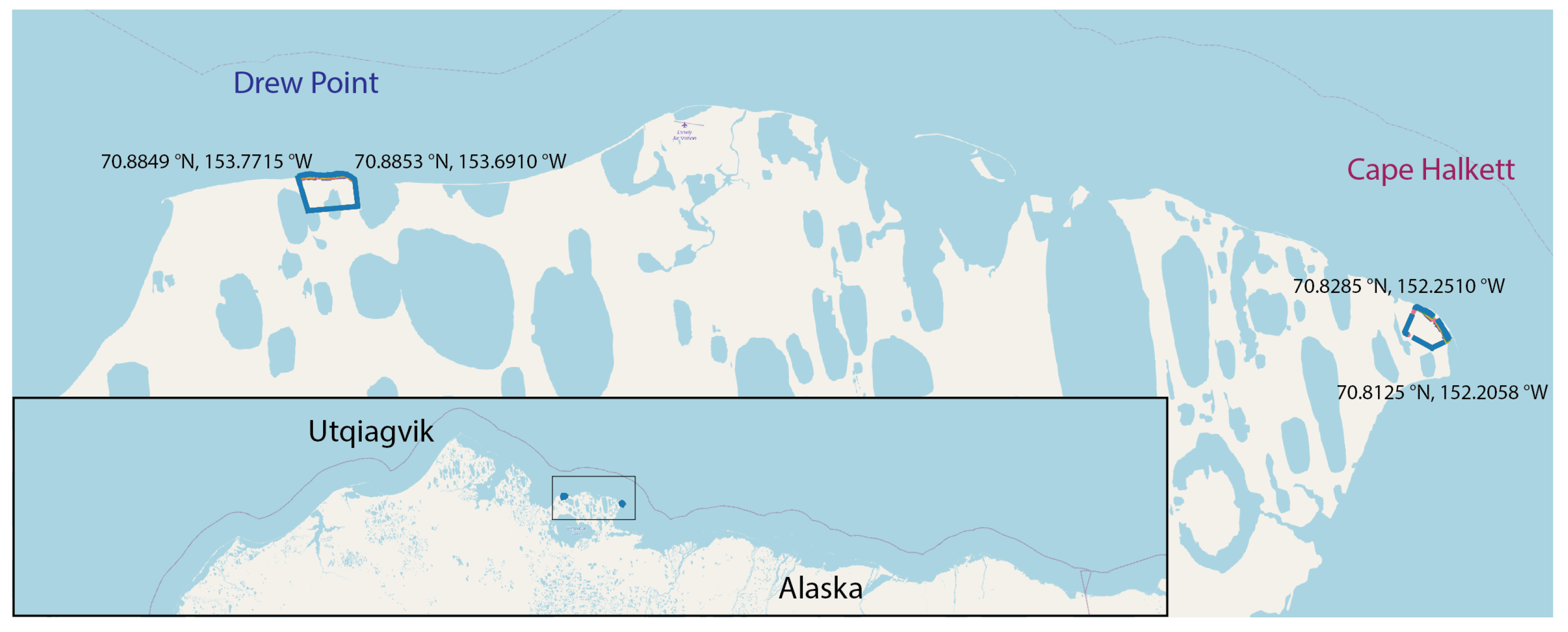
2.1. Study Sites

We selected two study sites from among locations identified as areas of particularly high erosion reported in the 2017 National Assessment of Shoreline Change [8]. From this set of locations, the Drew Point and Cape Halkett areas had reasonable availability of satellite imagery. Drew Point and Cape Halkett are particularly vulnerable to erosion because of the high ice content and fine sediment grains of their permafrost bluffs, as well as the absence of any protective barrier islands, and long-term erosion rates have been observed there as high as 17.1 m per year [27]. At both Drew Point and Cape Halkett, we selected 2–3 km of relatively straight coastline. Figure 1 shows the two sites relative to northern Alaska: the region is heavily ponded permafrost tundra.

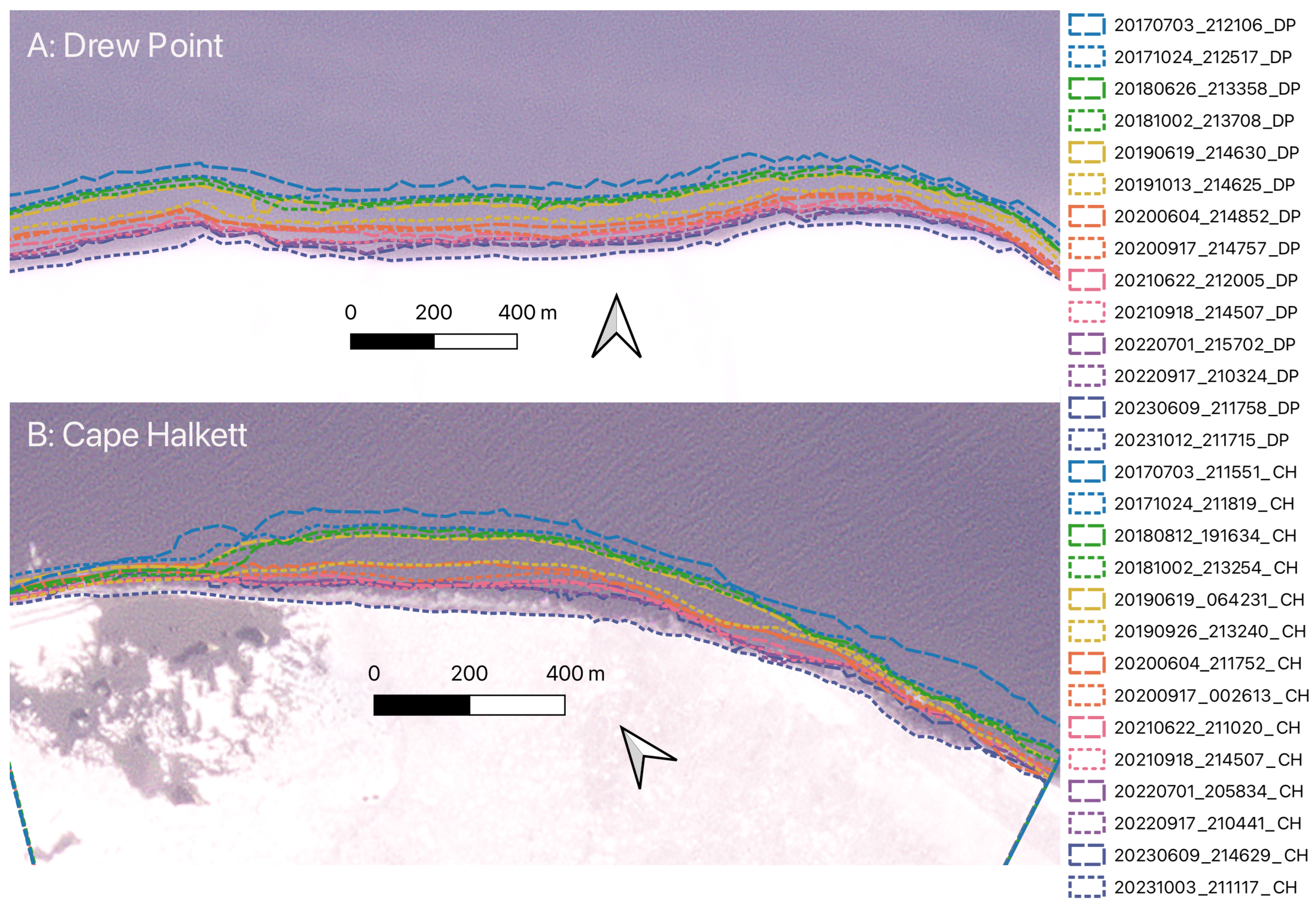
2.2. PlanetScope Imagery Analysis

We calculated erosion rates using high-resolution satellite imagery obtained from Planet under an educational and research license. Planet owns and operates over 140 satellites, offering 5 m resolution images of the Alaskan Arctic dating back to 2009. With the large constellation, Planet satellites have a high likelihood of being able to capture an image on the few available cloud-free days. Higher-spatial-resolution (3 m) imagery is only available in the area of our study sites beginning in 2017. Changing between the two spatial resolutions introduces geolocation errors, and prior to 2017 the constellation was too limited to obtain sufficient cloud-free images in the area for this analysis. To find cloud-free images, we set Planet’s cloud cover filter to 60% to maximize images retrieved (ice and snow often being mistaken for clouds) and followed up with visual inspection. For the highest available resolution (3 m), we selected images from 2017–2023 from the 4-band visual satellite images from PlanetScope [45]. In each frame collected by Planet’s 2D frame detector, a Bayer pattern filter and a “2-stripe” filter are used to capture both red, green, and blue (RGB, with wavelengths of 590–670 nm, 500–590 nm, and 455–515 nm, respectively) and near-infrared (780–860 nm) wavelengths. When the RGB half of the frame is combined with the NIR half of an adjacent frame, the result is the 4-band image [45]. We only use the RGB bands for this analysis.

In order to determine summer and winter erosion rates for each year, we selected from the earliest and latest available cloud-free PlanetScope images from the calendar year. For the purposes of this study, summer erosion rates are those calculated between the first available image of the summer and the last available image of a summer. Winter erosion rates are the rate of erosion calculated between the last available image of one summer and the first available image of the following calendar year. Figure 2 shows the season limits for each year (2017–2023) of the study: the earliest images at each site date to mid-June to early July, except for the Cape Halkett Site in summer 2018, which had no cloud-free images until early August. Dates earlier than mid-June are not reliable for detecting the shoreline, defined as the interface between tundra and water, as sea ice is indistinguishable in the imagery from snowy land surfaces. The latest image for each year dates between mid-September and mid-October, depending on cloud cover. Despite their proximity, sometimes the date of the earliest or latest image differed between the two sites because of broken cloud cover.

By using images near the beginning and end of the ice-free summer season, we measure a change in shoreline position between each image and calculate the seasonal erosion rate. Figure 3 shows these shoreline positions from 2017–2023. The images we used for analysis, both for the beginning and end of summer, were almost always collected between 1:00–2:00 p.m. AKST (21:00–22:00 UTC). This aligns with the maximum available sunlight at the end of the summer season (September–October). The early summer images are collected during a time of year with 24 h sunlight at these locations.

The early-summer images typically captured the beginning of the ice-free summer season within a couple of weeks in either direction. The late-summer images left a longer gap between the last image and estimated freeze-up dates. With a higher likelihood of storms and lower regional sea ice extents in the fall, the delay between the last image and freeze-up in the fall is most likely to cause problems in this analysis. Measured erosion rates (see Section 3.1) show little evidence of any significant erosion being counted as ‘winter’ instead of ‘summer’, with the possible exception of Fall 2020. This year had one of the latest images (October 12), so it is likely that this was a late-season storm rather than an error in the approach. Storms in October to December, prior to the stabilization of shore-fast ice, are known to cause winter erosion (e.g., Hertz [47]).

Satellite images were analyzed using QGIS 3.34 [48] using a WGS84 Ellipsoid for distance and area calculations. All images were georeferenced in QGIS and checked with ground control points (a selection of inland permafrost polygons and ponds) to ensure relative positional accuracy. We used 4–5 ground control points at each site, selected to be sufficiently inland from the coast that they were not at risk of erosion, and chosen by looking for features that were clearly recognizable in both snow and summer conditions. We traced the coastline manually and, whenever possible, traced bluffs instead of beachfront to reduce variability associated with tide level. At 3 m resolution, the transition from water to land could be visually identified to within 2–3 pixels accuracy in the absence of cloud cover. In this area, tides are very small (approximately 20 cm mean tidal range [49]) and tidal variability well within the water-to-land transition pixels. In order to ensure accuracy and consistency, each image has been traced multiple times by multiple people, but the final shorelines used were all traced by one individual.

Coastal length was calculated as the length of a trace mid-way between the earliest and the latest coastlines, with none of the small-scale (<10 m) wobbles in the real coastline. For each image, we created a polygon with two inland ground control points and the traced coastline. Seasonal erosion total was then area change divided by length, and daily erosion rate was that total divided by the number of days between images. The presence of sea ice rubble along the shoreline in the early summer can complicate detection of the coast location. By measuring area change between images, relatively small nicks (a few meters) out of the coast due to tracing around ice rubble are averaged out over the relatively long stretch (2+ km) of coastline.

Estimates of uncertainty on the erosion are calculated based on the precision with which the coastline can be traced from image to image: there is a little bit of blurring between pixels, and the coastline can sometimes only be determined to within 2–3 pixels. At 3 m per pixel, this could result in up to 9 m of horizontal error, which is equivalent to an error of 7.2–11.5 cm/day in the summer season and 3.1–3.6 cm/day in the longer winter season. Spatial registration of the images has a similar level of precision: the ground control points aligned in the images to within what we could discern visually. While there have been some issues with the accuracy of PlanetScope geolocation in the past [44], here we only need consistency between subsequent images because we do not combine PlanetScope imagery with other imagery sources. Checking control features for alignment is sufficient to constrain relative uncertainty over the 2–3 km lengths of shoreline we were considering: over longer stretches of coastline, further correction might be necessary. In practice, measurement error is likely smaller than 3 pixels because bias in one direction at one location is likely to be offset by bias in another direction elsewhere along the section of coastline. We include the full error estimate in the erosion rates presented in Figure 4.

2.3. Other Environmental Parameters

We used several additional data products for comparison between measured erosion rates and local and regional environmental parameters. Surface air and wind data come from the MERRA2 Reanalysis product [50]: zonal (u) and meridional (v) wind speeds at 10 m above surface level and 2m air temperature (Ta) are averaged over the area from 71° to 75°N and 200° to 210°E (−150° to −160°W) for each month in the 2017 to 2023 period. Sea surface temperature estimates come from the Hadley Centre Sea Ice and Sea Surface Temperature data set (HadISST), and are averaged over the same area. We retrieved the MERRA2 and HadISST products through the NOAA Physical Science Laboratory Climate Plotting and Analysis Tools subsetting tools [51]. Regional ice concentration data for comparison are the Sea Ice Index, Version 3, Northern Hemisphere Monthly Regional Sea Ice Area product [52], Beaufort Sea regional ice area. This product is accessed via the National Snow and Ice Data Center.

The Supplemental data file contains monthly data for all of these environmental parameters along with detailed retrieval instructions. The subsetting tool (NOAA-ESRL [51]) performs the spatial and temporal averaging before data are made available to download, so the retrieval instructions are slightly complicated. For variables considering the number of days above a threshold, we use the NCEP Reanalysis data product [53] for easier daily time-series extraction through the NOAA Physical Science Laboratory Climate Plotting and Analysis Tools [54]. Here we use daily 1000 mb-level air temperature and u- and v- wind to calculate the number of days exceeding a threshold (10 °C) for air temperature, 5 m/s for moderately windy days 10 m/s for high-wind days). We tested a number of thresholds before settling on these three. Again, the Supplemental data file includes specific access instructions for each of these products.

In total, we consider nine environmental parameters (labels indicated in parentheses): monthly mean 2 m air temperature ($T_a$), number of days above 10 °C ($T_a$ > 10 °C), monthly mean meridional wind speed (U), monthly mean zonal wind speed (V), monthly mean wind speed (WS), number of days with daily mean wind speed exceeding 5 m/s (WS > 5 m/s), number of days with daily mean wind speed exceeding 10 m/s (WS > 10 m/s), sea surface temperature (SST), and Beaufort Sea sea ice area (SIA). For parameter and each month of the year, we calculate the Pearson correlation coefficient between the parameter that month ($X_M$) and the summer erosion rate for each site ($R_{site}^S$), where $\sigma$ indicates the standard deviation.

$${\rho }_{X_M,R_{site}^S}=\frac{Cov(X_M,R_{site}^S)}{{\sigma }_{X_M}{\sigma }_{R_{site}^S}}$$

(1)

Because we are considering a small number of years (seven summers) of data, we use the p-value for each of these calculated correlation coefficients (measure of the probability of finding a particular correlation coefficient in this size sample of two unrelated variables). We consider p-values less than 0.05 (5%) to be significant.

3. Results

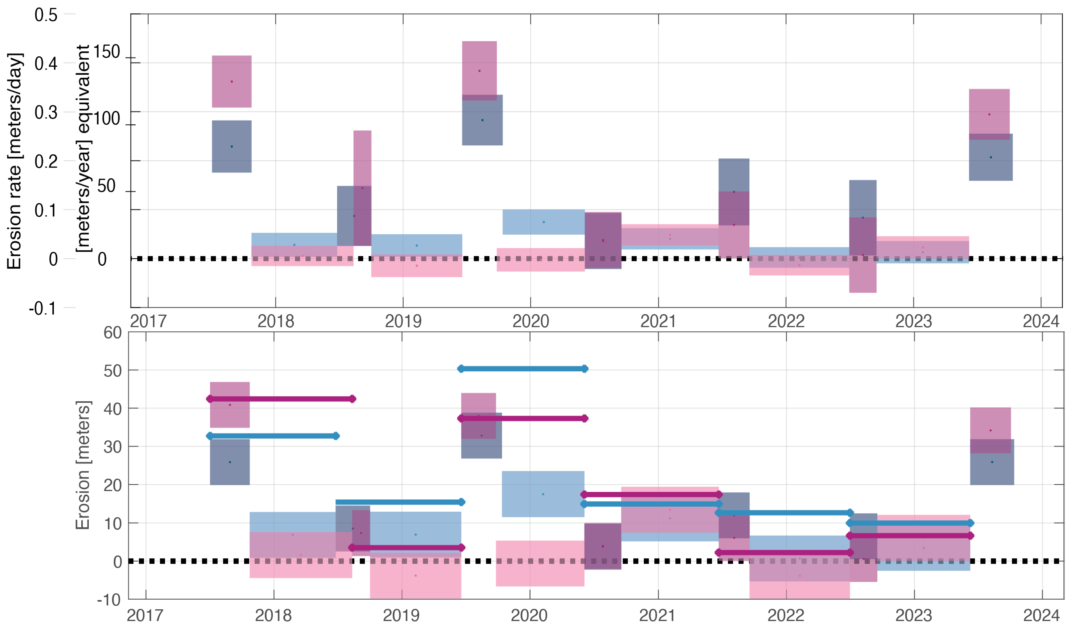
3.1. Measured Erosion Rates

Erosion rates calculated in this study range from over 30 cm/day in summers 2017 and 2019 at Cape Halkett (approximately equivalent to 120 m/year) to within the error margin of 0 in most of the winters. Figure 4 shows these rates and measured erosion totals for both sites: blue boxes indicate erosion rates measured at Drew Point and pink boxes are rates at Cape Halkett. The center dot of each box shows the measured erosion rate, and the vertical height of each box shows measurement uncertainty. Horizontal width of the box show the period over which the erosion rate was calculated. The lower panel shows erosion totals, with the annual total erosion at each site indicated by the horizontal line.

Summer erosion rates at both sites show significant variability: in low years, erosion rates are mostly between 0 and 15 cm/day; and in high years, erosion rates exceed 20 or even 30 cm/day. Winter erosion rates are consistently low, below 10 cm/day, and usually within error of 0 cm/day erosion across both sites. Cape Halkett shows slightly more interannual variability than the Drew Point erosion rates, which are lower in the high-erosion years and usually equivalent or higher in the low-erosion years. Annual erosion totals (solid bars in the lower panel) are likewise highly variable, accounting for both the large-magnitude variability of the summer erosion rates and the occasionally significant winter erosion events.

The highest winter rate at Drew Point (8 cm/day for 18 total meters in 2019–2020) was measured during a year in which the last pre-winter coastline image was at the early end of the range (17 September) and may have included an erosion event from late September or early October that in other years would have been included in the summer season. The relatively high winter erosion only happened at Drew Point, even though the Cape Halkett imagery dates were the same, suggesting that it was localized or directional event.

The average annual erosion over 2017–2023 was 22.7 m/year at Drew Point and 18.3 m/year at Cape Halkett. This exceeds the erosion recorded at Drew Point by previous studies: 17.1 m/year Ravens et al. [27], 17.2 m/year Jones et al. [46], and 7.1 m/year Gibbs and Richmond [8], though the latter used a longer transect.

Summer erosion rates between the two sites are highly correlated (0.92 correlation coefficient), suggesting that erosion during the ice-free summer season is driven by regional environmental factors rather than stochastic processes. Sea ice retreat (leading to higher fetch and more potential wave activity) and synoptic-scale storms could both have this effect, as could overall regional temperatures leading to thawing permafrost. Winter erosion rates are poorly correlated (0.15 correlation coefficient), indicating that the limited wintertime erosion tends to be more random in nature.

Validation of these erosion rate measurements is challenging: we use Planet imagery because they are the highest-temporal-frequency images with sufficient spatial resolution available in the region. Annual erosion totals are comparable to previous studies [8,46] that have used a variety of measurement approaches, lending credence to this approach. Jones et al. [46] reported a similar 22.0 m/year open water season erosion rate in 2007, 2012, and 2016 at Drew Point. Likewise, Gibbs and Richmond [8] documented short-term (1980s–2010s) maximum erosion rates of 25.1 m/year over the whole Beaufort Sea coast and 24.4 m/year between Drew Point and the Ikpikpuk River Delta, an area essentially equivalent to our study region. A more expansive study using this approach would benefit from a dedicated validation effort, including field surveys of coastline position at the beginning and end of the summer ice-free season.

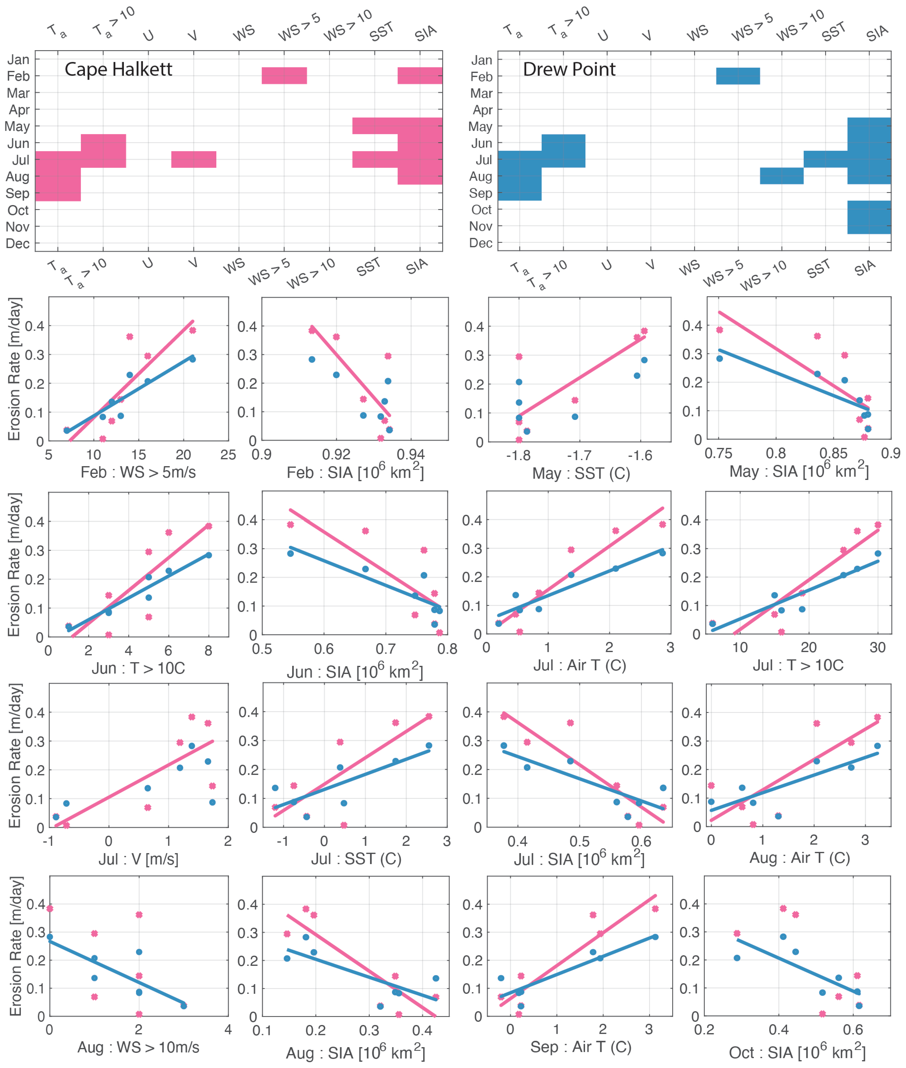
3.2. Correlation with Environmental Parameters

Figure 5 compares the seven summers of erosion rates at Drew Point (blue) and Cape Halkett (pink) to monthly mean air temperatures ($T_a$), the number of days with particularly warm temperatures ($T_a$ > 10 °C), westerly wind speeds (U), southerly wind speeds (V), wind speeds (WS), number of moderately windy days (above 5 m/s mean wind speed, WS > 5), number of highly windy days (above 10 m/s mean wind speed, WS > 10), sea surface temperatures (SST), and Beaufort sea ice area (SIA). The top panels show which parameters and at which months of the year show a statistically significant correlation (p < 0.05) with each of the sites with a highlighted block. For these significant correlations, the tiled panels show the environmental parameter for that particular month on the x-axis and the summer erosion rates at both sites on the y-axis. Where there is a statistically significant correlation between the two, a linear fit is shown in the color-coded line.

Overall, air temperatures (and the number of very warm days) and Beaufort sea ice area are the parameters most likely to show significant correlations. Air temperature is more likely to have an impact later in the summer (July–September), when shore ice is either breaking up or entirely absent. The number of really warm days matters more slightly earlier (June–July), around the time the shore is breaking up. Sea ice area in the Beaufort matters more earlier in the summer (May–August). This corresponds to times of year when decreasing sea ice area would contribute to increasing fetch and degrading shore ice (May–June) and when extended ice-free summer seasons would lead to warmer upper ocean temperatures resulting from a longer period of solar absorption (July–August).

Air temperatures in the late-summer months of July, August, and September were highly correlated with summer erosion rates at both sites. The number of warm days (defined as mean daily temperature above 10 °C) is correlated with erosion rate at both sites in June and July.

There is little relationship between wind speeds, in any direction or in magnitude, and erosion rates, with few exceptions. The number of days in February with wind speeds above 5 m/s are correlated with erosion rates at both sites, but this relationship does not hold for the number of days with higher (>10 m/s) winds. Southerly winds in July are correlated with erosion rates at Cape Halkett. There is a negative correlation between the number of high wind days (>10 m/s) in August and Drew Point erosion rates. Given the small number of years (seven summers) in the data set, some spurious correlations are likely, but the February correlation seems robust. This would correspond to a time of year in which shore-fast ice develops grounded ridges which help stabilize it into the summer melt season [55].

July sea surface temperature is positively correlated with erosion rate at both sites. Sea ice area in the Beaufort Sea (SIA) is negatively correlated (more ice cover leads to less erosion) at both sites from May through August. This correlation does not reach statistical significance in September, though Drew Point erosion rate is again negatively correlated with Beaufort sea ice area in October and November. This is after the late-summer image, which means that the early-winter ice area likely is influenced by similar processes to those driving erosion rates. Coastal sea ice in this area has persisted into June but not July in recent years [52], so this pattern reflects the state of the broader Beaufort sea ice rather than the loss of coastal ice.

4. Discussion

The results of this study support the observations that there is substantial seasonal variation in erosion rates along Alaska’s north coast and that there is significant variability between years. Summer erosion rates generally exceed winter erosion rates. The high interannual variability means that the bulk of erosion over the period comes from a limited number of summer seasons, with smaller changes in coastline position in the winters and other summers. Given the sheer magnitude of the difference between high erosion summers and other seasons and the consistency between our two study locations, this pattern seems likely to generalize across permafrost bluff shorelines in the Arctic.

Several environmental factors show strong correlations with summer erosion rate. Sea ice area in the Beaufort sea is a good indicator for the early- and mid-summer season (May–August). There are several mechanisms by which the amount of sea ice in the region this time of year could be influencing erosion rates: decreased ice area increases fetch, breakup of shore-fast ice leaves shorelines exposed, and the decreasing duration of summertime sea ice coverage leads to warmer water temperatures, which could accelerate thermal degradation of permafrost bluffs. That the relationship with SST is much less robust (only a significant correlation in July) suggests that the thermal mechanism is not the predominant effect. There is some relationship however, and there may be a limit to how well a reanalysis product can capture near-surface water temperatures in the area. In situ measurements would be necessary to further explore this mechanism. Limited correlations with wind speeds in the region suggest that variability in fetch is not a major driver either. Neither wind speeds or number of days above a wind speed threshold are robustly correlated with erosion rates, even in the months with minimal sea ice cover in the area. Coastal and shore-fast sea ice as a protective barrier is not addressed directly in this study, but seems likely to be a major determinant of summer erosion rates.

Air temperature in the area across the later summer (July–September) and number of hot days in the earlier summer (June–July) are both highly correlated at both sites. This suggests that thawing permafrost is also a major factor and warm summers contribute to accelerating coastal erosion. With climate models projecting continued decreases in regional sea ice cover [56] and increasing air temperatures [57] across the Arctic, it is likely that the high-erosion summers will be common in the future.

It is also important to note that beyond the seasonal variation, our results underscore that coastal erosion in these two locations is occurring on a truly massive scale—as high as 50.3 m and 42.4 m in the highest total annual erosion at Drew Point and Cape Halkett, respectively. These are average eroded area across 2–3 km of shoreline—not simply spots where individual blocks have collapsed—and are among the highest annual erosion rates known to be recorded in the Alaskan Arctic [8]. However, there may be other areas across the Arctic coast with similarly concerning rates. At an average rate of 20 m/year, over 500 additional meters of coastal tundra at Drew Point and Cape Halkett would be lost by the year 2050.

Although the present results clearly indicate seasonal variation in coastal erosion and the severity of erosion more generally at Drew Point and Cape Halkett, it is nevertheless important to recognize that this analysis considers only two 2–3 km sections of coastline on the relatively small timescale of 7 years. These rates should be kept in the context of larger-scale and longer-duration studies. At Drew Point and Cape Halkett, 3 m resolution images do not exist from Planet further back than 2017, but high-resolution images exist from other sources and for other sites (e.g., Jones et al. [46]). This effort has specific implications for the study of coastal erosion using remote sensing products, given the recent improvements in availability of the high-resolution satellite imagery. This imagery can be a valuable tool in measuring erosion on shorter timescales and across larger geographic scales than was previously possible.

Jones et al. [46] highlighted the need for higher-temporal-resolution erosion measurements in order to determine the factors controlling coastal erosion rates along permafrost bluff coastlines in the Arctic. This study achieved that on a small scale: measurements of erosion rates on a seasonal timescale, rather than annual or longer, show statistically significant relationships with environmental parameters linked to the major mechanisms thought to drive coastal erosion in the region. We demonstrate the viability of PlanetScope imagery as a tool for coastal erosion research in the region: high temporal frequency is necessary for sufficiently cloud-free imagery in the region. Our results show high interannual and seasonal variability in coastal erosion rates, with over 40 m of erosion happening in a single summer at Cape Halkett. This kind of catastrophic erosion—between years of more modest coastal losses—underscores the pressing need to understand the mechanisms driving alarmingly high summer erosion rates.

References

1. Hino, M.; Field, C.B.; Mach, K.J. Managed retreat as a response to natural hazard risk. Nat. Clim. Chang. 2017, 7, 364–370. [Google Scholar] [CrossRef]
2. MacDougall, A.H.; Avis, C.A.; Weaver, A.J. Significant contribution to climate warming from the permafrost carbon feedback. Nat. Geosci. 2012, 5, 719–721. [Google Scholar] [CrossRef]
3. Johannessen, O.M.; Bengtsson, L.; Miles, M.W.; Kuzmina, S.I.; Semenov, V.A.; Alekseev, G.V.; Nagurnyi, A.P.; Zakharov, V.F.; Bobylev, L.P.; Pettersson, L.H.; et al. Arctic climate change: Observed and modelled temperature and sea-ice variability. Tellus A Dyn. Meteorol. Oceanogr. 2004, 56, 328–341. [Google Scholar] [CrossRef]
4. Overeem, I.; Anderson, R.S.; Wobus, C.W.; Clow, G.D.; Urban, F.E.; Matell, N. Sea ice loss enhances wave action at the Arctic coast. Geophys. Res. Lett. 2011, 38, 1–6. [Google Scholar] [CrossRef]
5. Nicholls, R.J.; Marinova, N.; Lowe, J.A.; Brown, S.; Vellinga, P.; De Gusmao, D.; Hinkel, J.; Tol, R.S. Sea-level rise and its possible impacts given a `beyond 4 C world’ in the twenty-first century. Philos. Trans. R. Soc. A Math. Phys. Eng. Sci. 2011, 369, 161–181. [Google Scholar] [CrossRef]
6. Casas-Prat, M.; Wang, X.L. Projections of Extreme Ocean Waves in the Arctic and Potential Implications for Coastal Inundation and Erosion. J. Geophys. Res. Ocean. 2020, 125, 1–18. [Google Scholar] [CrossRef]
7. Lantuit, H.; Overduin, P.P.; Couture, N.; Wetterich, S.; Aré, F.; Atkinson, D.; Brown, J.; Cherkashov, G.; Drozdov, D.; Forbes, D.L.; et al. The Arctic coastal dynamics database: A new classification scheme and statistics on Arctic permafrost coastlines. Estuaries Coasts 2012, 35, 383–400. [Google Scholar] [CrossRef]
8. Gibbs, A.E.; Richmond, B.M. National Assessment of Shoreline Change: Summary Statistics for Updated Vector Shorelines and Associated Shoreline Change Data for the North Coast of Alaska, US-Canadian Border to Icy Cape; US Department of the Interior, Geological Survey: Reston, VA, USA, 2017.
9. Gibbs, A.E.; Snyder, A.G.; Richmond, B.M. National Assessment of Shoreline Change—Historical Shoreline Change along the North Coast of Alaska, Icy Cape to Cape Prince of Wales; Technical Report; US Geological Survey: Reston, VA, USA, 2019.
10. Lantuit, H.; Pollard, W. Fifty years of coastal erosion and retrogressive thaw slump activity on Herschel Island, southern Beaufort Sea, Yukon Territory, Canada. Geomorphology 2008, 95, 84–102. [Google Scholar] [CrossRef]
11. Ogorodov, S.; Aleksyutina, D.; Baranskaya, A.; Shabanova, N.; Shilova, O. Coastal erosion of the Russian Arctic: An overview. J. Coast. Res. 2020, 95, 599–604. [Google Scholar] [CrossRef]
12. Jones, B.M.; Arp, C.D.; Jorgenson, M.T.; Hinkel, K.M.; Schmutz, J.A.; Flint, P.L. Increase in the rate and uniformity of coastline erosion in Arctic Alaska. Geophys. Res. Lett. 2009, 36. [Google Scholar] [CrossRef]
13. Mars, J.; Houseknecht, D. Quantitative remote sensing study indicates doubling of coastal erosion rate in past 50 yr along a segment of the Arctic coast of Alaska. Geology 2007, 35, 583–586. [Google Scholar] [CrossRef]
14. Casas-Prat, M.; Wang, X.L. Sea ice retreat contributes to projected increases in extreme Arctic Ocean surface waves. Geophys. Res. Lett. 2020, 47, e2020GL088100. [Google Scholar] [CrossRef]
15. Are, F. Thermal abrasion of sea coasts (parts I and II). Polar Geogr. Geol. 1988, 12, 1–157. [Google Scholar] [CrossRef]
16. Stroeve, J.; Serreze, M.; Drobot, S.; Gearheard, S.; Holland, M.; Maslanik, J.; Meier, W.; Scambos, T. Arctic sea ice extent plummets in 2007. Eos Trans. Am. Geophys. Union 2008, 89, 13–14. [Google Scholar] [CrossRef]
17. Richter-Menge, J.; Overland, J.E. (Eds.) Arctic Report Card 2010; National Oceanic and Atmospheric Administration: Washington, DC, USA, 2010. Available online: http://www.arctic.noaa.gov/reportcard (accessed on 18 June 2024).
18. Steele, M.; Ermold, W.; Zhang, J. Arctic Ocean surface warming trends over the past 100 years. Geophys. Res. Lett. 2008, 35, 1–6. [Google Scholar] [CrossRef]
19. Brown, J.; Romanovsky, V.E. Report from the International Permafrost Association: State of permafrost in the first decade of the 21st century. Permafr. Periglac. Process. 2008, 19, 255–260. [Google Scholar] [CrossRef]
20. Jorgenson, M.T.; Shur, Y.L.; Pullman, E.R. Abrupt increase in permafrost degradation in Arctic Alaska. Geophys. Res. Lett. 2006, 33, 1–4. [Google Scholar] [CrossRef]
21. Jorgenson, M.; Yoshikawa, K.; Kanevskiy, M.; Shur, Y.; Romanovsky, V.; Marchenko, S.; Grosse, G.; Brown, J.; Jones, B. Permafrost characteristics of Alaska. In Proceedings of the Ninth International Conference on Permafrost, Fairbanks, AK, USA, 29 June–3 July 2008; University of Alaska Fairbanks: Fairbanks, AK, USA, 2008; Volume 3, pp. 121–122. [Google Scholar]
22. IPCC. Contribution of Working Groups I, II and III to the Fourth Assessment Report of the Intergovernmental Panel on Climate Change. In Climate Change 2007: Synthesis Report; Core Writing Team, Pachauri, R.K., Reisinger, A., Eds.; IPCC: Geneva, Switzerland, 2007. [Google Scholar]
23. Wobus, C.; Anderson, R.; Overeem, I.; Matell, N.; Clow, G.; Urban, F. Thermal erosion of a permafrost coastline: Improving process-based models using time-lapse photography. Arctic Antarct. Alp. Res. 2011, 43, 474–484. [Google Scholar] [CrossRef]
24. Dallimore, S.R.; Wolfe, S.A.; Solomon, S.M. Influence of ground ice and permafrost on coastal evolution, Richards Island, Beaufort Sea coast, NWT. Can. J. Earth Sci. 1996, 33, 664–675. [Google Scholar] [CrossRef]
25. Benumof, B.T.; Storlazzi, C.D.; Seymour, R.J.; Griggs, G.B. The relationship between incident wave energy and seacliff erosion rates: San Diego County, California. J. Coast. Res. 2000, 16, 1162–1178. [Google Scholar]
26. Atkinson, D.E. Observed storminess patterns and trends in the circum-Arctic coastal regime. Geo-Mar. Lett. 2005, 25, 98–109. [Google Scholar] [CrossRef]
27. Ravens, T.M.; Jones, B.M.; Zhang, J.; Arp, C.D.; Schmutz, J.A. Process-based coastal erosion modeling for drew point, North Slope, Alaska. J. Waterw. Port Coastal Ocean. Eng. 2012, 138, 122–130. [Google Scholar] [CrossRef]
28. Mason, O.K.; Jordan, J.W. Heightened North Pacific storminess during synchronous late Holocene erosion of Northwest Alaska beach ridges. Quat. Res. 1993, 40, 55–69. [Google Scholar] [CrossRef]
29. Sturtevant, P.M.; Lestak, L.R.; Manley, W.F.; Maslanik, J.A. Coastal erosion along the Chukchi coast due to an extreme storm event at Barrow, Alaska. Arctic Coastal Dynamics, Report of an International Workshop. Available online: https://www.researchgate.net/publication/242132406_COASTAL_EROSION_ALONG_THE_CHUKCHI_COAST_DUE_TO_AN_EXTREME_STORM_EVENT_AT_BARROW_ALASKA (accessed on 18 June 2024).
30. Radosavljevic, B.; Lantuit, H.; Pollard, W.; Overduin, P.; Couture, N.; Sachs, T.; Helm, V.; Fritz, M. Erosion and flooding—Threats to coastal infrastructure in the Arctic: A case study from Herschel Island, Yukon Territory, Canada. Estuaries Coasts 2016, 39, 900–915. [Google Scholar] [CrossRef]
31. Barnhart, K.R.; Overeem, I.; Anderson, R.S. The effect of changing sea ice on the physical vulnerability of Arctic coasts. Cryosphere 2014, 8, 1777–1799. [Google Scholar] [CrossRef]
32. Crawford, A.D.; Lukovich, J.V.; McCrystall, M.R.; Stroeve, J.C.; Barber, D.G. Reduced sea ice enhances intensification of winter storms over the Arctic Ocean. J. Clim. 2022, 35, 3353–3370. [Google Scholar] [CrossRef]
33. Fang, Z.; Freeman, P.T.; Field, C.B.; Mach, K.J. Reduced sea ice protection period increases storm exposure in Kivalina, Alaska. Arct. Sci. 2018, 4, 525–537. [Google Scholar] [CrossRef]
34. Stroeve, J.; Markus, T.; Boisvert, L.; Miller, J.; Barrett, A. Changes in Arctic melt season and implications for sea ice loss. Geophys. Res. Lett. 2014, 41, 1216–1225. [Google Scholar] [CrossRef]
35. Barrow Atmospheric Baseline Observatory. NOAA Global Monitoring Observatory: Wind Speed In Situ Meteorology Data, 1973–2024. Available online: https://gml.noaa.gov/dv/iadv/graph.php?code=BRW&program=met&type=ts (accessed on 25 May 2024).
36. Bliss, A.C.; Steele, M.; Peng, G.; Meier, W.N.; Dickinson, S. Regional variability of Arctic sea ice seasonal change climate indicators from a passive microwave climate data record. Environ. Res. Lett. 2019, 14, 045003. [Google Scholar] [CrossRef]
37. Cavalieri, D.J.; Parkinson, C.L. Arctic sea ice variability and trends, 1979–2010. Cryosphere 2012, 6, 881–889. [Google Scholar] [CrossRef]
38. Guégan, E.B.; Christiansen, H.H. Seasonal Arctic coastal bluff dynamics in Adventfjorden, Svalbard. Permafr. Periglac. Process. 2017, 28, 18–31. [Google Scholar] [CrossRef]
39. Vos, K.; Harley, M.D.; Splinter, K.D.; Simmons, J.A.; Turner, I.L. Sub-annual to multi-decadal shoreline variability from publicly available satellite imagery. Coast. Eng. 2019, 150, 160–174. [Google Scholar] [CrossRef]
40. Specht, M.; Specht, C.; Lewicka, O.; Makar, A.; Burdziakowski, P.; Dąbrowski, P. Study on the Coastline Evolution in Sopot (2008–2018) Based on Landsat Satellite Imagery. J. Mar. Sci. Eng. 2020, 8, 464. [Google Scholar] [CrossRef]
41. Esmail, M.; Mahmod, W.E.; Fath, H. Assessment and prediction of shoreline change using multi-temporal satellite images and statistics: Case study of Damietta coast, Egypt. Appl. Ocean. Res. 2019, 82, 274–282. [Google Scholar] [CrossRef]
42. USGS. What Are the Band Designations for the Landsat Satellites? United States Geological Survey: Reston, VA, USA, 2022.
43. Tatem, A.J.; Goetz, S.J.; Hay, S.I. Fifty years of earth observation satellites: Views from above have lead to countless advances on the ground in both scientific knowledge and daily life. Am. Sci. 2008, 96, 390. [Google Scholar] [CrossRef]
44. Frazier, A.E.; Hemingway, B.L. A Technical Review of Planet Smallsat Data: Practical Considerations for Processing and Using PlanetScope Imagery. Remote Sens. 2021, 13, 3930. [Google Scholar] [CrossRef]
45. Planet Labs PBC. Planet Application Program Interface: In Space for Life on Earth, 2017–2023; Planet Labs PBC: San Francisco, CA, USA, 2024; Available online: https://api.planet.com (accessed on 25 May 2024).
46. Jones, B.M.; Farquharson, L.M.; Baughman, C.A.; Buzard, R.M.; Arp, C.D.; Grosse, G.; Bull, D.L.; Günther, F.; Nitze, I.; Urban, F.; et al. A decade of remotely sensed observations highlight complex processes linked to coastal permafrost bluff erosion in the Arctic. Environ. Res. Lett. 2018, 13, 115001. [Google Scholar] [CrossRef]
47. Hertz, N. Alaska Gov. Walker declares disaster after costly fall storm on North Slope. Anchorage Daily News, 15 November 2017. [Google Scholar]
48. QGIS.org. QGIS Geographic Information System. 2022. Available online: https://qgis.org (accessed on 18 June 2024).
49. NOAA. Tides and Currents: Tide Predictions 9095048 Point Barrow, AK; National Oceanic and Atmospheric Administration: Washington, DC, USA, 2024. Available online: https://tidesandcurrents.noaa.gov/noaatidepredictions.html?id=9495048&units=metric&bdate=20240301&edate=20240331&timezone=LST/LDT&clock=12hour&datum=MLLW&interval=hilo&action=data (accessed on 18 June 2024).
50. GMAO. MERRA-2 instM_3d_ana_Np: 3d, Monthly Mean, Instantaneous, Pressure-Level, Analysis, Analyzed Meteorological Fields V5.12.4 (M2IMNPANA), 2m Air Temperature, 10m u-wind, 10m v-wind; Global Modeling and Assimilation Office: Greenbelt, MD, USA, 2015. [Google Scholar] [CrossRef]
51. NOAA-ESRL. Web-Based Reanalysis Intercomparison Tool: Monthly Maps; Physical Sciences Laboratory: Boulder, CO, USA, 2024. Available online: https://psl.noaa.gov/data/atmoswrit/map/ (accessed on 18 June 2024).
52. Fetterer, F.; Knowles, K.; Meier, W.N.; Savoie, M.; Windnagel, A.K. Sea Ice Index, Version 3; National Snow and Ice Data Center: Boulder, CA, USA, 2017. [Google Scholar] [CrossRef]
53. Kalnay, E.; Kanamitsu, M.; Kistler, R.; Collins, W.; Deaven, D.; Gandin, L.; Iredell, M.; Saha, S.; White, G.; Woollen, J.; et al. The NCEP/NCAR 40-year reanalysis project. Bull. Am. Meteorol. Soc. 2018, 77, 437–472. [Google Scholar] [CrossRef]
54. NOAA-ESRL. Access and Analyze Daily Weather/Climate Time Series; Physical Sciences Laboratory: Boulder, CO, USA, 2024. Available online: https://psl.noaa.gov/data/timeseries/daily/ (accessed on 18 June 2024).
55. Mahoney, A.; Eicken, H.; Gaylord, A.G.; Shapiro, L. Alaska landfast sea ice: Links with bathymetry and atmospheric circulation. J. Geophys. Res. Ocean. 2007, 112, 1–18. [Google Scholar] [CrossRef]
56. Jahn, A.; Holland, M.M.; Kay, J.E. Projections of an ice-free Arctic Ocean. Nat. Rev. Earth Environ. 2024, 5, 164–176. [Google Scholar] [CrossRef]
57. Overland, J.E.; Wang, M.; Walsh, J.E.; Stroeve, J.C. Future Arctic climate changes: Adaptation and mitigation time scales. Earth Future 2014, 2, 68–74. [Google Scholar] [CrossRef]
Figure 1. Map of the area around the two study sites, Drew Point and Cape Halkett, with an inset showing their location relative to the North Slope of Alaska. Coordinates indicate the east and west ends of the two coastline sections considered in this study.
Remotesensing 16 02365 g001
Figure 2. Dates of images used for the analysis at Drew Point (left) and Cape Halkett (right). Dotted lines indicate the over-winter period and solid lines indicate the summer period. Early summer images are generally close to the ice breakout dates, while late summer images typically leave a month or more before the onset of freeze-up.
Remotesensing 16 02365 g002
Figure 3. Coastline traces for (A) Drew Point and (B) Cape Halkett. Coastlines are color-coded by year, with dashed lines for fall images and dotted lines for spring images. The legend indicates the date (YYYYMMDD) and image number for each trace.
Remotesensing 16 02365 g003
Figure 4. (Top) Calculated erosion rates marked as center points in m/day and m/year equivalent at each of the two locations (Drew Point in blue and Cape Halkett in pink) during summer and winter seasons. Vertical height of the boxes indicate measurement uncertainty in erosion, and horizontal width shows the period of time over which erosion was calculated. (Bottom) boxes indicate total measured erosion over each season, with annual totals indicated by the bold lines. Solid lines indicate annual erosion totals at each site.
Remotesensing 16 02365 g004
Figure 5. (Top) highlighted cells indicate which environmental parameters at each month of the year show a statistically significant correlation with summer erosion rates at Cape Halkett (pink) and Drew Point (blue), including surface air temperature (Ta), days above 10 °C (Ta > 10), zonal wind (V), meridional wind (U), wind speed (WS), days with mean wind speeds above 5 m/s (WS > 5), days with mean wind speeds above 10 m/s (WS > 10), sea surface temperature (SST), and Beaufort sea ice area (SIA). (Below) Individual panels showing the relationship between the monthly environmental parameters (x-axis) and erosion rates at both sites. Solid lines indicate statistically significant correlations at that site. Panels are in order of month.
Remotesensing 16 02365 g005
Disclaimer/Publisher’s Note: The statements, opinions and data contained in all publications are solely those of the individual author(s) and contributor(s) and not of MDPI and/or the editor(s). MDPI and/or the editor(s) disclaim responsibility for any injury to people or property resulting from any ideas, methods, instructions or products referred to in the content.