Pre-Earthquake Oscillating and Accelerating Patterns in the Lithosphere–Atmosphere–Ionosphere Coupling (LAIC) before the 2022 Luding (China) Ms6.8 Earthquake

Abstract

The coupling processes among the lithosphere, atmosphere, and ionosphere (LAI) during the earthquake preparation phase are still an open scientific debate. Comprehensive LAI coupling effects around the 2022 Ms6.8 Luding earthquake in China are investigated with a multi-parameter and multi-layer approach, including the b-value, revised accelerated moment release, Earth resistivity, ELF magnetic field emissions, atmospheric electric field, surface temperature, foF2 from ionosonde, GNSS TEC, Ne and magnetic field from CSES and Swarm satellites, and energetic electrons from CSES and NOAA satellites. It is found that the anomalies start from the lithospheric parameters as Earth resistivity and b-values 1–2 years before to reflect the local stress loading in the seismic region, then the ionospheric and atmospheric disturbances occur and accelerate −50 days before and −15 days before, and finally the electrons precipitate a few days before. The simultaneous perturbations in LAI illustrate the thermodynamic coupling channel, such as on 24 August, −12 days before. Meanwhile, the abundant developed ionospheric anomalies without atmospheric disturbances demonstrate the electromagnetic coupling way from the lithosphere to the ionosphere directly. Finally, the results demonstrate a two-way model of LAIC: one way is characterized by a slow chain of processes, of thermodynamic nature, starting from the ground and proceeding to the above atmosphere and ionosphere, showing an exponential trend in the cumulative number of anomalies; the second way is characterized by oscillating electromagnetic coupling between the lithosphere and ionosphere, showing intermittent fluctuations in the corresponding cumulative number of anomalies.

1. Introduction

Due to the significant earthquake-related perturbations observed in the ionosphere by ground-based stations and space-borne satellites, scientists have increasingly focused on studying the possible coupling mechanism among the lithosphere, atmosphere, and ionosphere, also known as lithosphere–atmosphere–ionosphere coupling (LAIC). In the LAIC model, Hayakawa (2004) [1] proposed three channels, namely the chemical channel (also known as the electric field channel), the acoustic gravity wave (AGW) channel, and the electromagnetic (EM) channel, to establish connections between different observations in each layer. Pulinets and Ouzounov (2011) [2] presented a more unified LAIC model, taking the radon emission as the basic source of coupling from the lithosphere. They focused on the formation of an abnormal electric field in the atmosphere, which they linked to the formation of an anomalous electric field in the ionosphere, inducing irregularities in the magnetosphere and particle precipitation related to very low frequency (VLF) signals [2]. To simplify the simulation models, the coupling channels from Hayakawa [1] are more widely used. In the context of the electric field channel, Kuo et al. (2011, 2014) [3,4] developed a model to calculate the current penetrating from the lithosphere into the ionosphere and the disturbances induced by this overlapping electric field. In this model, they observed perturbations in Total Electron Content (TEC) ranging from 10 to 20%, with simultaneous disturbances occurring in the conjugate region. Additionally, Zhou et al. (2018) [5] simulated the coupling process of the electric field among the lithosphere, atmosphere, and ionosphere, finding that the electric field more readily penetrated higher latitudes with greater intensity, while the penetration height was lower at lower latitudes. Concerning the AGW channel, Carbone et al. (2021) [6] developed a numerical model to depict the processes wherein the ground motion, including Love and Rayleigh waves, induces disturbances in lower atmospheric pressure or density, subsequently propagating into the upper atmosphere through AGW mode. Gao et al. (2023) [7] proposed a method to simulate AGWs in the atmosphere and ionosphere using a point force on the Earth’s surface. This method explored two modes: high-frequency acoustic waves and low-frequency gravity ones. In the high-frequency mode, three apparent horizontal velocities were identified, i.e., sound-speed acoustic wave, head wave with P-wave velocity, and head wave with Rayleigh wave velocity. In the low-frequency mode, observations revealed a gravity wave just above the source and a Lamb wave that rapidly decayed with altitude. In the EM channel between the lithosphere and ionosphere, numerous simulations have been conducted across a broad frequency band. Molchanov et al. (1995) [8] presented a model for EM emissions from the seismic source to the ionosphere in the range of 0.01–100 Hz. Their findings indicated that only the signals from a magnetic-type source penetrated the magnetosphere, generating Alfven waves, with the intensity of 1–10 $\mathsf{\mu }\mathrm{V}/\mathrm{m}/\sqrt{\mathrm{H}\mathrm{z}}$ in the electric field and 1–10 pT/$\sqrt{\mathrm{H}\mathrm{z}}$ in the magnetic field, and a horizontal scale of 100–200 km. Bortnik and Bleier (2004) [9] proposed a full-wave propagation model, accounting for the oblique geomagnetic field, to facilitate the penetration of ultra-low-frequency (ULF) and extremely low-frequency (ELF) EM waves. Ozaki et al. (2009) [10] employed a similar full-wave model to compute EM waves within the frequency band of 10 Hz–1 kHz, confirming that the primary intensity of EM waves originated from whistler waves propagating along the magnetic field and the ground-ionosphere waveguide. Zhao et al. (2021) [11] simulated the underground propagation of ELF waves using a whistler wave mode into the ionosphere, potentially detectable in the electric field within 100–300 Hz by satellites when the lithosphere conductivity is lower and the focal depth is shallow, approximately 10 km. Due to the need to simplify the boundary conditions in models, differences or significant errors persist between the model and real observations.

The coupling mechanism from the earthquakes and ionospheric disturbances is quite complex, with multiple channels contributing at different preparation stages or even simultaneously. To verify the LAIC processes, multi-parameter analysis around earthquakes has become a hot topic, involving different parameters at various layers, and employing diverse observing technologies within the same layer. De Santis et al. (2020) [12] analyzed several parameters from the lithosphere, atmosphere, and ionosphere on occasion of the 2019 Ridgecrest earthquake, finding an accelerated progression of the cumulative number of all anomalies as the mainshock was approaching. For the same earthquake, Xie et al. (2021) [13] detected some precursors using the TEC from global navigation satellite system (GNSS) receivers, and electron density (Ne) and electron temperature (Te) data from China Seismo-EM Satellite (CSES) and Swarm satellite missions. They found them to be consistent with the coupling process of the electric field channel. De Santis et al. (2022) [14] presented a comprehensive analysis, collecting data in the lithosphere, atmosphere, and ionosphere around two strong earthquakes, i.e., the Kermadec Islands and Ridgecrest earthquakes. Two kinds of LAIC were suggested: one for the direct propagation of electric current, and another for thermodynamic diffusion to the atmosphere and the ionosphere, possibly related to AGWs. To illustrate the electric field action in the LAIC mechanism, recent research has also considered atmospheric electric field (AEF) observations [15,16]. Yang et al. (2019) [17] focused on AGWs by investigating disturbances in atmospheric temperature profiles at the middle atmosphere and demonstrated the relationship between stratospheric AGW activity and sub-ionospheric VLF observations before earthquakes. Piersanti et al. (2020) [18] suggested an AGW/GW model to link observations from the atmosphere to the ionosphere with disturbances in Ne and enhancements of field-line resonance in the magnetic field detected by satellites. Concerning EM wave coupling, numerous anomalies have been detected at ground stations and satellites around strong earthquakes [19,20,21,22], but the direct propagation processes from the lithosphere to the ionosphere still have not been validated to be from the same source, primarily due to the lack of simultaneous observations for EM emissions at the ground and in the ionosphere.

On 5 September 2022, an earthquake with a magnitude of Ms6.8 occurred in Luding, Sichuan Province, China, at 102.08°E, 29.59°N, with a focal depth of 16 km (China Earthquake Networks Centre, CENC), with heavy cloud coverage over the epicenter and its surrounding region before and after the event. Inverting the seismic data, a rupture model for this seismic event was found showing that the earthquake released a seismic moment of 1.12 × 10¹⁹ Nm, corresponding to a moment magnitude of Mw 6.6 [23]. The epicenter was located in the Y-type region intersected by the Xianshuihe fault, Longmenshan fault, and Anninghe fault. The focal mechanism indicated a pure strike-slip motion [24], with the fault plane striking 163° and dipping at 77° (southwestward), and a rake of −5°. The typical mainshock–aftershock sequence was proposed for this earthquake from the following values of indices obtained: the b-value of the Gutenberg–Richter frequency–magnitude relationship was 0.81, the h-value and p-value of the Omori’s law were 1.4 and 1.21, respectively, and finally a magnitude of completeness of 1.41 was obtained [25]. Several papers have been published about the geophysical or geochemical precursors of this earthquake. Jing et al. (2023) [26] utilized microwave brightness temperature (MBT) and clear-sky outgoing longwave radiation (ClrOLR) data to identify thermal anomalies around the Luding earthquake, and prominent signals were detected over the epicenter within two months before the event. Lu et al. (2023) [27] summarized soil gas observations along the Xianshuihe, Anninghe, and Zemuhe faults: a typical increase was observed in H₂, CH₄, and CO₂ in 2022 relative to the values in 2019 and 2021, particularly at the Yanzigou station, closest to the Luding earthquake epicenter. Wu et al. (2024) [16] investigated four stations with AEF observations around the Luding seismic region within 15 days before the earthquake. After removing the anomalies affected by meteorological factors, four anomalies occurring on 22 August, 24 August, and two on 5 September (just a few hours before the mainshock), respectively, were confirmed to be related to this earthquake. Chen et al. (2023) [28] analyzed multi-observations mainly at the Leshan station, located 175 km from the Luding earthquake epicenter. Abnormal signals were detected in seven geophysical parameters about 3 h before the event, including ground tilts, air pressure, radon concentration, atmospheric vertical electric field, geomagnetic field, wind field, and TEC. The chemical channel and atmospheric resonance were suggested during the coupling process.

There are many available observations over the 2022 Luding Ms6.8 earthquake, which provide a good opportunity to construct the internal relationship among multiple parameters in different layers during the earthquake preparation stage. This paper will present a comprehensive analysis of the lithospheric, atmospheric, and ionospheric data to confirm the temporal and spatial evolution processes of seismic-related anomalies among different layers. The coupling mechanism will be discussed using multiple observations based on their internal physical property and energy transfer paths.

2. Data Source

For the study of LAIC processes, specific datasets are required to validate the different channels. In considering the standardization of different parameters, the spatial scale is constrained using the equation of $\mathsf{\rho }={10}^{0.43\mathrm{M}}$ [29], relating the strain radius ρ in km of a supposed circular area of the preparation region of the earthquake with magnitude M. The time period of the analysis extends to 90 days before the earthquake for most parameters.

2.1. Lithospheric Data

Because Sichuan Province is prone to earthquakes, there is a dense seismic network which can detect the micro-earthquakes with a magnitude smaller than 1.0. To calculate the b-values and the revised accelerated moment release (R-AMR) [30] in the Luding seismic region, earthquakes with a magnitude larger than 1.0 were selected around the Y-type areas crossing with the Xianshuihe, Longmenshan, and Anninghe faults.

To detect EM precursors, a lot of technologies have been set up in China, including Earth resistivity, geomagnetic field, geoelectric field, EM emissions, ELF EM field, etc. The Earth resistivity is sensitive to the variations in crustal strain and stress, which always showed the turning of a long-term variational trend and short-term acceleration before strong earthquakes [31]. Around the Luding earthquake, the data on resistivity have been collected since 2016 at four stations to present the long-term changes in the seismic region and the possible short-term changes related to strong earthquakes with a magnitude larger than 6.0 in the neighboring region. The geomagnetic field data are widely used in earthquake research, and many kinds of anomalies have been reported before earthquakes [19,20,32], in which the transfer function helps to confirm the underground source signals when the vertical component is larger than the horizontal one [20,33]. In China, the geomagnetic field observations have a long history of more than 30 years, and, only in Sichuan Province, about 10 geomagnetic stations are operating. For the ELF band, the typical EM waves are Schumann Resonance, and Hayakawa et al. (2021) [34] showed that this kind of anomaly is related to two Japanese earthquakes. Of course, the atmospheric radiation in the ULF and ELF bands of the magnetic field are also reported before earthquakes [35]. Since 2021, nine magnetic field stations have been built in Sichuan Province, with an observing frequency band of 0.003~20 Hz, a sampling rate of 100 Hz, a noise level of ≤0.5 pT/Hz 1/2 at 1 Hz, and sensitivity of ≥5 mV/nT at 0.5~20 Hz. So, around the Luding seismic region, the EM observing technologies are numerous at the ground.

2.2. Atmospheric Data

The electric field is a major channel for the LAIC mechanism. To monitor the electric field variations, more than 30 stations for AEF have been installed in Sichuan Province, China, with a resolution of 5 V/m and a sampling rate of 1 s. Most stations were constructed at the end of 2020, with some of them quite near to the Luding earthquake (i.e., within 50 km, so they totally cover the epicentral area and the time period of earthquake occurrence). As we know, the AEF is heavily affected by meteorological factors [15], and the clear days in Sichuan Province are always fewer each year, so the meteorological data with a sampling rate of 1 h are also collected at the nearest stations to AEF ones.

According to the LAIC model [2], some atmospheric variables are expected to be anomalously related to the preparation phase of earthquakes. Therefore, they have been simultaneously processed in order to identify possible persistent atmospheric anomalous days before the impending earthquakes. The Climatological Analysis for seismic PRecursor Identification (CAPRI) algorithm [36] has been applied to the ECMWF-ERA (European Centre of Medium range Weather Forecast-Re-Analysis) climatological dataset with a spatial grid of 0.25° × 0.25°.

After collection and preprocessing of time series, we then apply the CAPRI algorithm, which compares daily time series of the investigated year to the past forty-year historical series in a time window of some months preceding the seismic event. If the observable exceeds with certain persistence (say, at least two days), the mean of the time series by twice the standard deviation, an anomaly is identified.

The ECMWF Re-Analysis v5 (ERA5) dataset provides hourly estimates of a large number of atmospheric, land, and oceanic climate variables. We focused on physical variables related to the thermal radiative interaction of the atmosphere with the surface, skin temperature (SKT), and Outgoing Longwave Radiation (OLR). The data cover the Earth on a 30 km grid and resolve the atmosphere using 137 levels from the surface up to a height of 80 km. In our case, we limited the analysis to the epicentral region of the Luding earthquake.

2.3. Ionospheric Data

Multi-technologies can monitor the ionosphere for different parameters, both from ground and from satellites. From the ground, ionosonde measurements can detect the critical frequency of the F2 layer (foF2), the height (hmF2) of the main Ne peak, and also the information of the sporadic E (Es) layer (such as its critical frequency foEs), which can represent the variations in F and E layers. Over the Luding earthquake, three ionosonde stations are included, with Puer (22.7°N; 101.05°E; 770 km from the Luding earthquake epicenter) and Tengchong (24.98°N, 98.51°E; 624 km far) in Yunnan Province, and Daofu (31.0°N; 101.12°E) in Sichuan Province, which is the closest one to the epicenter (182 km far). The TEC can be obtained by integrating Ne in the cylinder of a 1 m² cross section from GNSS satellites to the receivers at the ground. On the mainland of China, about 260 continuous global positioning system (GPS) and 170 GNSS receivers have been set up to monitor the crustal deformation, which can be used to obtain the TEC time series over each station. In addition, to illustrate the spatial characteristics, especially the local distribution or the conjugate features, the GIM TEC is also widely used in the study of earthquakes [37], where the data published by CODE are collected with a high time resolution of 1 h and a spatial resolution with 2.5° × 5° in latitude and longitude (http://ftp.aiub.unibe.ch/CODE/, accessed on 4 April 2012).

Meanwhile, satellites can detect the in situ plasma parameters and electromagnetic field. CSES (also named CSES-01 or ZH-1 because the first of a series of CSES/ZH satellites; data are published at https://leos.ac.cn/#/dataService/dataBrowsingList after registration, accessed on 1 October 2018) was launched in 2018, with a sun-synchronous orbit at the altitude of 507 km and a node time at LT14:00 and LT02:00. Onboard CSES, eight payloads were installed, with EFD to detect the three-component electric field from DC to 3.5 MHz, HPM and SCM for the magnetic field, LAP to measure electron density and temperature (Ne and Te), PAP for ions (Ni, Ti, Vi, etc.), HEPP and HEPD for energetic particles, and GOR and TBB to detect the TEC and Ne profiles [38]. So, multiple parameters from CSES can be used in the study of the Luding earthquake. Meanwhile, the three Swarm satellites (Alpha, Bravo, and Charlie) have been operated since November 2013 by ESA, with data published in the magnetic field, Ne, Te, TEC, etc. (https://swarm-diss.eo.esa.int/ accessed on 1 September 2023).

By combining the above satellites, we can compare and follow the signals in the same parameters in the magnetic field or Ne at different altitudes, which provides a good opportunity for us to link the signals possibly from the same source. Satellite magnetic data coming from the ESA Swarm mission have been analyzed using the MASS (MAgnetic Swarm anomaly detection by Spline analysis) methodology for magnetic data and the NeAD (Electron density, Ne, Anomaly Detection) method [39]. These techniques are used to detect electromagnetic anomalies from Swarm magnetic field data (Level 1B, low resolution of 1 Hz) and electron density data (Level 1B, with 2 Hz sampling rate). These methods are based on the analysis of the three components of the geomagnetic field (X, Y, Z) and intensity (F) (MASS) or the electron density (NeAD) for every track of the satellite (Swarm A, Swarm B, Swarm C). The analysis consists in the determination of the first differences of the time series (dX/dt, dY/dt, dZ/dt, dF/dt, dNe/dt) and the removal of the long trend using a cubic spline. Moreover, it is important to evaluate the quality of the data using the quality flags provided by ESA, considering only magnetic quiet times (|Dst| | ≤ 20 nT and ap ≤ 10 nT) and excluding polar regions (±50° geomagnetic latitudes) because they are very disturbed. After this analysis, we compare the root mean square (rms) of sliding windows of 7° shifting every 1.4° with the whole root mean square of the track (RMS). When the RMS is greater than kt times the value of RMS, this window is classified as anomalous. For satellite magnetic data, kt is established as 2.5 and for electron density, kt is established as 3.0, following previous works yet to be published [40].

NOAA satellites have been circling the Earth’s orbit since the 1980s and have utilized a shared instrument for detecting charged particles since 1998. The Medium-Energy Proton and Electron Detector (MEPED) installed on NOAA satellites is equipped with eight solid-state detectors designed to measure proton and electron counting rates (CRs) within the 30 keV–200 MeV range [40]. These measurements encompass radiation belt populations, energetic solar proton events, and the low-energy segment of the galactic cosmic-ray population. Specifically, the two telescopes for electrons detected three energy bands ranging from 30 keV to 2.5 MeV. One telescope observes at a 9° angle, oriented towards the local zenith, while the second telescope provides an orthogonal view at 90° along the satellite motion for the local zenith. The compact solid-state detectors possess nominal geometric acceptances of 0.1 cm²sr and opening angle apertures of ±15°. Since geomagnetic activity is the main driver of electron loss, periods during which the ap index exceeded a threshold were omitted from the analysis, with the ap index varying according to the season and year due to the solar cycle. Fidani (2021) [41] investigated a statistically significant correlation between excesses in electron CRs and strong seismic events in the West Pacific up to 35° latitude above the land. CR excesses were selected as having a <1% probability of being Poissonian fluctuations. The observed correlation appeared 1.5–3.5 h before the occurrence of mainshocks. It was particularly prominent when considering earthquakes with depths shallower than 200 km. Meanwhile, HEPP and HEPD payloads have been installed on CSES, to detect the energy band of 0.1~50 MeV for electrons and 2~200 MeV for protons, which can make a comparison and supplement for the NOAA satellite.

3. Analysis Methods and Results

3.1. The Seismological Data Analysis

3.1.1. b-Value

The temporal variation in the b-value analysis along the Moxi fault was investigated to appreciate the changes in the seismicity pattern before and the first days after the Luding earthquake.

The b-value is a parameter of the Gutenberg–Richter (G–R) law [42]. The G–R equation, given by logN(M) = a − bM, describes the number of earthquakes, N(M), with a magnitude equal or greater than a threshold M, as a function of their magnitude M. In the G–R equation, a and b are parameters whose values may change in space and time. The total number of earthquakes of M ≥ 0 is given by the a-value while the b-value describes the frequency distribution of earthquakes with a smaller magnitude relative to those of larger magnitude: a large b-value corresponds to a high frequency of small events. Some studies suggest that its variation is related to the differential stress state in the Earth’s crust [43,44,45,46]. Therefore, the temporal heterogeneity of the b-value can be considered a prominent tool for strong earthquake forecasting [47,48,49].

In this study, we performed the temporal b-value analysis on seismic data drawn from CENC. The seismic data were retrieved in the period from 1 January 2012 to 28 October 2023 with a magnitude range between 0 and 7.0 and a depth lower or equal to 42 km. The delimited area (lat. 29.3°–30.4° and long. 101.5°–102.4°) along the seismogenic structure contains 26,567 events. We obtained a magnitude completeness value, Mc, equal to 1.3, from which and above, it included 90% of the data [50], thus reducing the catalog to 10,231 events.

Figure 1 shows the temporal variation in the b-value from 1 January 2012 to 28 October 2023. It is possible to observe a sharp decrease in the b-value starting from 17 November 2021, i.e., 292 days prior to the Luding earthquake. This behavior may be associated with strong stress accumulation along the nearby fault, indicating a potential impending rupture [47].

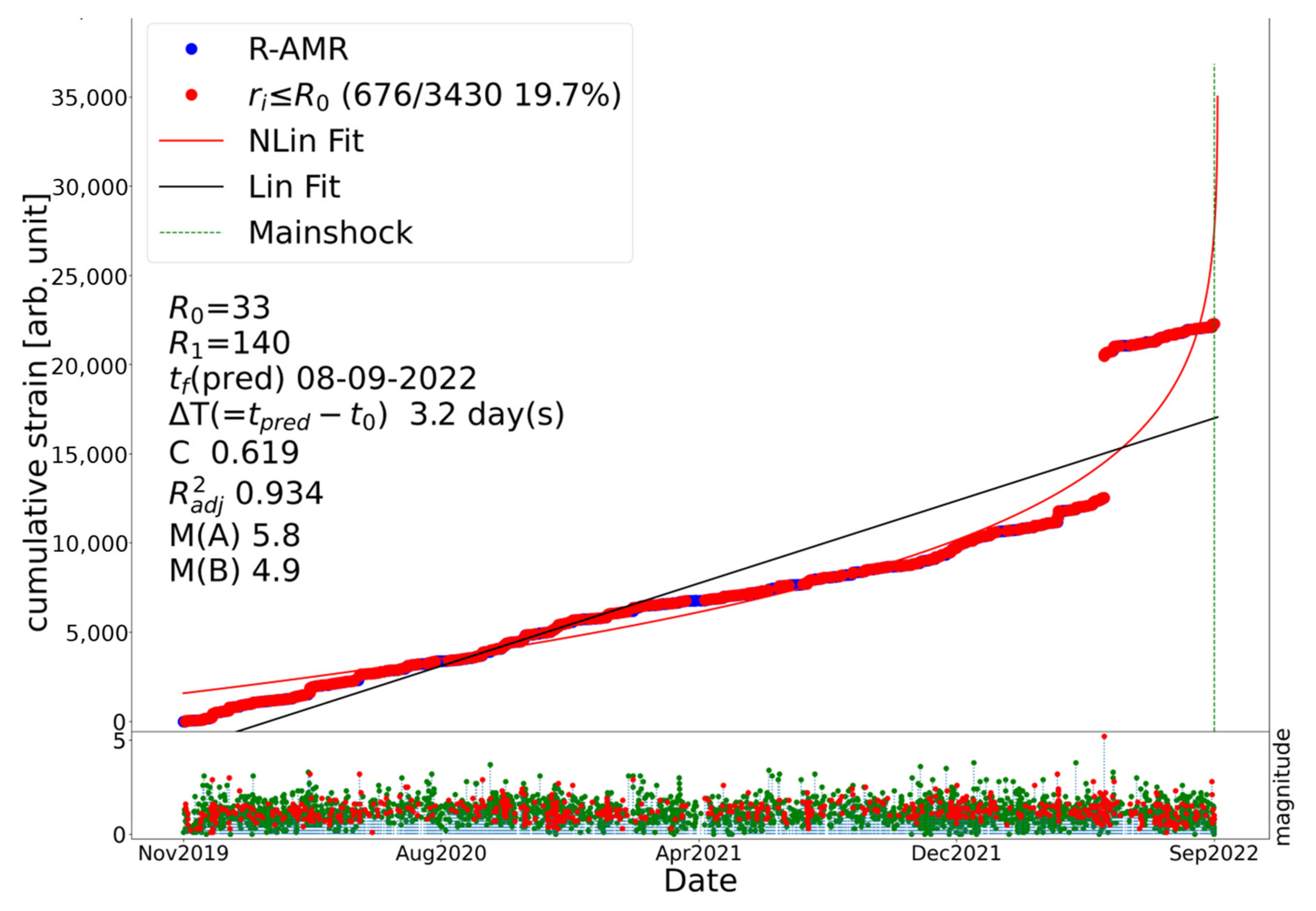
3.1.2. R-AMR Analysis

Although not always present in seismic sequences, several studies [51] indicate that when the right conditions are respected [52], then accelerated seismicity may be observed during the preceding phase of large earthquakes.

Explained in terms of the Critical Point Theory, where the mainshock is assimilated to a phase transition reached at a so-called time-to-failure ${\mathrm{t}}_{\mathrm{f}}$, this feature of seismicity recorded around the impending mainshock area may be undisclosed in the catalogue; it may emerge and be detected thanks to the method called “Accelerated Moment Release (AMR)”, and particularly by its recent revised version, called R-AMR, when it is applied to earthquake catalogues [30,53]. We then applied the R-AMR algorithm to the CENC catalogue in the region around the Luding earthquake.

A way to measure acceleration in seismicity is through the inspection of the cumulative seismic Benioff strain ${\mathrm{s}}_{\mathrm{i}}=\sqrt{{\mathrm{E}}_{\mathrm{i}}}$ as follows: each seismic event releases a strain proportional to the square root of its energy ${\mathrm{E}}_{\mathrm{i}}={10}^{\left(1.5{\mathrm{M}}_{\mathrm{i}}+4.8\right)}$ [J]. The cumulative of the strain, i.e., the quantity $\mathrm{s}\left(\mathrm{t}\right)=\sum {\mathrm{s}}_{\mathrm{i}}$, is called the Cumulative Benioff Strain. As explained [30,54], it expresses the regional increase in the cumulative Benioff deformation $\mathrm{s}\left(\mathrm{t}\right)$ before a large shock through the power-law time-to-failure functional relation:

$$\mathrm{s}\left(\mathrm{t}\right)=\mathrm{A}+\mathrm{B}{\left({\mathrm{t}}_{\mathrm{f}}-\mathrm{t}\right)}^{\mathrm{m}}$$

where ${\mathrm{t}}_{\mathrm{f}}$ is the prediction of the occurrence of the mainshock (i.e., the phase transition) and m < 1 is an inverse measure of how quickly the acceleration grows around ${\mathrm{t}}_{\mathrm{f}}$.

With the aim of evaluating the quality of seismic acceleration with respect to a linear trend, the latter representing the cumulative deformation of random background seismicity, Bowman et al. (1998) [51] introduced a quantity called C-factor, which is defined as the ratio between the sum of the squares of the residuals of the power-law fit of s = s(t) and the same quantity of a linear fit. According to this definition, when C is less than 1, there is an acceleration; furthermore, the lower the C-factor, the more the acceleration characterizes the seismic sequence. Typical values of the C-factor range from 0.1 to 0.7.

A step forward in understanding and improving the technique was made by De Santis et al. (2015) [30], where the focus was on the strain deposited on the mainshock fault by the preceding seismicity around it, corrected by an appropriate damping function with distance. With the further improvement of the algorithm applied on 14 case studies [53], the robustness of the approach and algorithm was verified. It has been proven that it is capable of revealing the acceleration—when present but hidden in the sequence—providing an estimate of the time ${\mathrm{t}}_{\mathrm{f}}$ of occurrence of the mainshock (never included in the calculation) and of the expected magnitude, obtained from parameters A and B of the functional relation [30].

In the present analysis, the algorithm is automatic—considering the s = s(t) time series backward and excluding the mainshock, it detects the time when the acceleration starts, in this case, on the first of November 2019. Figure 2 shows the outcome of the R-AMR method applied to the seismic catalogue when considering the earthquakes occurred in a region of 140 km radius from the epicenter (see Figure 3). The C-factor (=0.62) gives an indication of acceleration in s(t), and also evidences the time-to-failure red curve with respect to the linear trend (black line). It is worth noticing that the predicted ${\mathrm{t}}_{\mathrm{f}}$ is very close to the actual origin time (their difference is only 3 days). The expected magnitudes M(A) and M(B), provided by the method, are instead underestimated with respect to the mainshock magnitude. A deeper visual inspection of Figure 2 leads to some more considerations. First, the fault area is marked by an almost continuous background seismicity—as shown by the red symbols representing the on-fault earthquakes with respect to the blue ones, which are out of the fault area. The second consideration is that the main driver of the accelerating behavior, which emerged from the analysis, is the significant M5.2 foreshock occurred on 20 May 2022, spatially close to the mainshock epicenter, which impressed a very steep jump to the cumulative.

3.2. The Electromagnetic Data Analysis on the Ground

3.2.1. Earth Resistivity

The Earth resistivity observation plays an important role in earthquake research, especially before strong earthquakes with a magnitude larger than 6 [56] or even larger than 7.0. The abnormal types include an abrupt change in the long-term variational trend, an enhancement or weakness, or even the disappearance of the annual variation amplitude, showing a positive correlation between the time duration and the earthquake magnitude. As shown in Figure 4, the annual variations are quite clear at each station, with peak values occurring in winter and valley values in summer. The turning of the long-term trend in resistivity was clear at all four stations since 2021, where at Ganzi (100.0°E, 31.6°N), it turned from a decrease to flat (Figure 4a,b), at Jiangyou (104.7°E, 31.8°N) and Hongge (101.9°E, 26.5°N), from an increase to flat (Figure 4c,d,g,h), and where Mianning (102.2°E, 28.5°N) (Figure 4e,f) was possibly the same as Jiangyou and Hongge. This means that the time duration of these anomalies in resistivity is about 600 days prior to the Luding earthquake. It should be paid attention to that, on the same day, i.e., 21 May 2021, the Yangbi Ms 6.4 and Maduo Ms 7.4 earthquakes took place one after the other in Yunnan and Qinghai Provinces, which may also have contributed to the anomaly construction in resistivity in Sichuan Province. However, after the Yangbi and Maduo earthquakes, all the anomalies continued and did not recover to the normal state they had before 2021, which could indicate another strong earthquake as Luding was preparing in this region. Another feature is that the peak duration time for 2022 became shorter and the resistivity decreased quickly in March or April with no recovery, such as NE (northeast direction) at Ganzi (Figure 4a), SN (South–North) and NW (Northwest) at Mianning (Figure 4e,f), and SN at Hongge (Figure 4c), while in other years, the fast decrease always occurred in the summer season, which is mainly due to the increase in the underground temperature and precipitation.

Figure 5 shows the comparison of resistivity and precipitation at three stations in 2022, which demonstrates the close relationship of precipitation and the quick decrease in resistivity at Hongge and Mianning in the summer season of May to September, while the resistivity at the Ganzi station did not present any instant decrease response with precipitation as the other two stations did. As for the turning decrease in resistivity in March or April (within yellow rectangles in Figure 5), it can be seen that Mianning had some precipitation in the spring season that may have contributed to that, but the Hongge station had almost no precipitation in these two months (Figure 5a,b); therefore, its quick turning from peak to decrease might have been caused mainly by the regional resistivity decreasing and the conductivity increasing, induced by the Luding earthquake preparation process, similar to what occurred at Ganzi (Figure 5d).

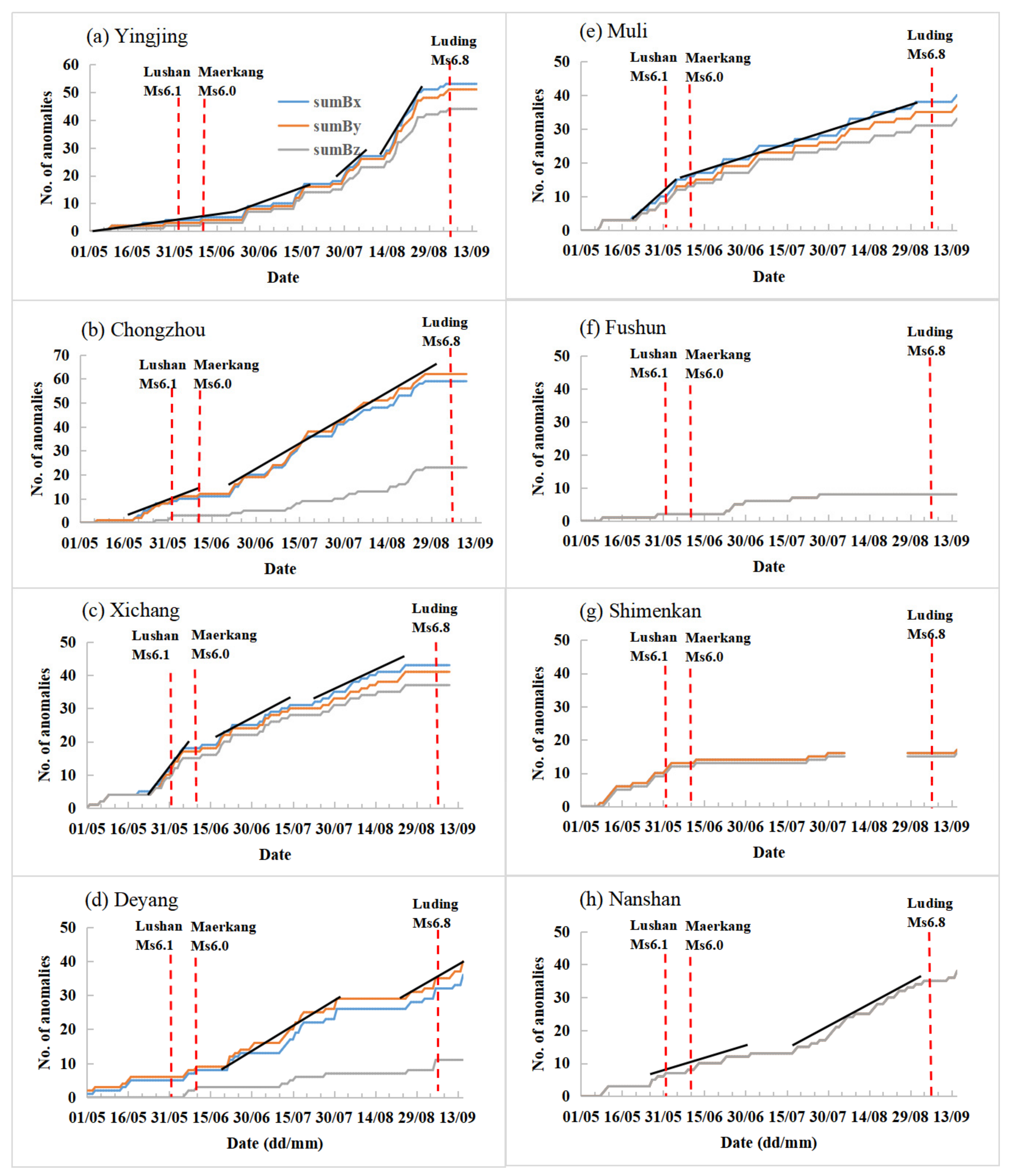
3.2.2. ELF Ground Magnetic Field

Observations from eight ELF magnetic field stations located in Sichuan Province have been analyzed with the Fast Fourier Transform (FFT) to get the spectrum, and the significant EM emissions were detected in a wide frequency band 1–2 orders higher in power spectrum density relative to the quiet background. The EM emissions were collected at each station, and the final numbers in eight stations were accumulated as shown in Figure 6 from 1 May to 13 September 2022. During this time period, two other earthquakes with magnitudes larger than 6.0 took place at Lushan and Maerkang in Sichuan Province, so they are also marked in this figure with the epicentral distance from each station. The results show that Yingjing station (102.8°E, 29.8°N), the nearest to the Luding earthquake with a distance of about 75 km, presented the quick increase in speed since the middle of June to the end of August, especially in the last half month of August (Figure 6a). The other five stations also exhibited a fast increase in anomaly numbers, including Xichang (102.6°E, 27.9°N), Muli (101.3°E, 27.9°N), Chongzhou (103.5°E, 30.8°N), Deyang (101.2°E, 30°N), and Nanshan (101.7°E, 26.5°N), among which Deyang presented the anomalies just around the Luding earthquake occurrence (Figure 6d). Only Shimenkan (102.8°E, 26.9°N), with a distance of 293 km, and Fushun (105°E, 29.3°N) within 186 km, show a flat and smooth trend around the Luding earthquake (Figure 6f,g).

Besides the EM emissions before the earthquake, the co-seismic signals were also detected at Yingjing station on 5 September 2022.

3.3. The Atmospheric Data Analysis

3.3.1. Atmospheric Electric Field from Ground

Over the epicentral area, AEF data at 26 stations were collected from 1 August to 10 September 2022, with the meteorological data at the nearest stations in Sichuan Province. To confirm the variations related to tectonic activity, four parameters were selected and well defined to remove the meteorological effects [15], in which the requirements all need to be satisfied at the same time: (1) no precipitation with rainfall = 0 mm; (2) visibility $\ge 20 \mathrm{km}$ with less dust or mist in the air; (3) a maximum wind speed of $<8 \mathrm{m}/\mathrm{s}$ to ensure the absence of strong wind; (4) humidity $<80\%$ with less mist. About the AEF, the normal diurnal amplitude in the AEF is about 100 V/m, so the anomalies are defined as amplitude $\ge$ 300 V/m with a time duration longer than 30 min.

Figure 7 gives an example for the anomaly distinguished in the AEF on 15 August 2022 at the stations within 50 km of the Luding earthquake epicenter, in which the meteorological data observed in Luding city were provided on the same day. It can be seen that some disturbances occurred at five stations, some of them being related to meteorological factors such as those at Caoke station around LT20:00 with a wind speed greater than 8 m/s (Figure 7b around LT20:00), but others, such as Lanan and Guzan at LT00-01, actually had less of a relationship with meteorological factors that were defined as AEF anomalies (Figure 7d,e). So, after removing the disturbances possibly related to meteorological conditions, the AEF data were scanned at each station, and all the possible seismic-associated anomalies were selected and summarized in Figure 8. Within a distance of 300 km to the Luding epicenter, 23 stations detected anomalies among the total 26, i.e., 88% of all stations, which means that the preparation process of the Luding earthquake affected the tectonic activity in a large region. As shown in Figure 8, two time intervals with AEF anomalies were detected frequently, one for 14–18 August, and one for 23–25 August, especially on 24 August, with the number of anomalies exceeding 2σ (σ being its standard deviation), nearly 50% with almost half of the 26 stations detecting disturbed signals in the AEF.

3.3.2. SKT and OLR

In order to analyze the ECMWF ERA5 time series, an area sensitive to earthquake energy, as established by the Dobrovolsky minimum strain radius [30], of around 7° in latitude × 7° in longitude around the epicenter was considered, and SKT and OLR over the region of interest were estimated, comparing the 2022 data with the historical time series of 42 years, from 1980 to 2021. Anomalies were extracted when they overcame the historical mean by 2$\mathsf{\sigma }$, according to the application of the CAPRI algorithm [36]. The estimated anomalies are all the more significant the longer they persist over time.

Figure 9 depicts the case study for the 2022 Luding Ms6.8 earthquake for two ECMWF SKT and OLR analyzed parameters. Each red oval puts in evidence the identified anomalous days (the values are taken in local nighttime to avoid the possible daily solar contamination). Colored stripes indicate 1.0 σ (light green), 1.5 σ (green), and 2.0 σ (yellow) from the mean of the historical time series, respectively. The earthquake occurred at the end of the analyzed period (vertical red line). On the right is the map of the day with the main anomaly. Both parameters revealed two-day persistence anomalies. In particular, SKT showed one anomaly starting on 24 August 2022, twelve days before the mainshock. It was shortly preceded by the 21 August OLR anomaly, although it was not the main one, that occurred previously on 7 July, together with a third persistent OLR anomaly occurring on 15 July.

The SKT spatial distribution of the main anomaly (Figure 9, top right) confirms the position of the maximum value close to the epicenter of the seismic event, in particular to the east. Looking at Figure 9 (bottom right), the OLR data spatial distribution shows the peak intensity of the main anomaly, which is located east of the epicenter.

3.4. The Ionospheric Data Analysis

3.4.1. GNSS TEC

The ionospheric perturbations have a close relationship with solar activity and magnetic storms. Here, some indices data were collected and the quiet days were defined as satisfying the following values of the geomagnetic and solar indices: Kp < 3, Dst > −30 nT, AE < 500 nT, F10.7 < 150 sfu, and no solar flare above M-level. The GPS TEC data located in the preparation zone of the Luding earthquake were analyzed with the IQR (Inter-Quartile Range) method according to Equation (1), where the TEC_o is the raw data with a sampling rate of 15 min and 96 points for each day at each station, TEC_m is the median of the previous 15 days at each point, and k = 1.5.

$$∆TEC=\left\{\begin{array}{c}{TEC}_o-({TEC}_m+kIQR) {TEC}_o>{TEC}_m+kIQR\\ 0 {TEC}_m-kIQR\le {TEC}_o\le {TEC}_m+kIQR\\ {{TEC}_o-(TEC}_m-kIQR) {TEC}_o<{TEC}_m-kIQR \end{array}\right.$$

(1)

After removing the effects from solar and geomagnetic activities, it was found that 23–26 August is a quiet time period for ionospheric data analysis. The GPS TEC time series showed a significant decrease on 26 August at the stations north of the Luding earthquake such as in Gansu and Qinghai Provinces (Figure 10a). To illustrate the spatial distribution of $∆TEC$ on 26 August, the $∆\mathrm{T}\mathrm{E}\mathrm{C}$ was plotted with a time interval of 2 h, in which, at UT06-08, the decreasing disturbances occurred north of the epicenter, and then at UT20-22, increasing perturbations with small amplitude were presented south of the epicenter in Yunnan Province (Figure 10b). Although these disturbances were mostly located in the seismic region of the Luding earthquake, no perturbations from the TEC were just over the epicenter; they were shifted to the north or south.

The GIM TEC published by CODE can also demonstrate the spatial distributions, including those in the magnetically conjugate ones. The same method as Equation (1) was employed to distinguish the anomalies in the GIM TEC. The decreasing anomalies in the GIM TEC were both shown at UT06-10 on 24 and 26 August at the southern area and covering the epicenter, and on 24 August, the disturbances at the northern hemisphere near the epicenter were much larger than the conjugate one at the southern hemisphere (Figure 11a). Due to the conjugate propagation characteristics of signals in the ionosphere, not only can the perturbations be detected at the conjugate region, but earthquakes at the conjugate region can induce the ionospheric disturbances over China. In this case, western Indonesia is just conjugate with Yunnan and Sichuan in China, so the Indonesian earthquakes should be considered to analyze these anomalies. Before the Luding earthquake occurrence, an Indonesian earthquake with Ms6.1 took place on 29 August, whose location is consistent with the anomalies at the southern hemisphere on 26 August and the conjugate area in southern China. Figure 11 chose the column data at longitude 100–105 °E to show the $∆\mathrm{T}\mathrm{E}\mathrm{C}$ with latitudes of −30°S to 40°N from 1 July to 11 September 2022. All the earthquakes with a magnitude larger than 6.0 in conjugate regions were marked with the epicenter latitudes (red star) and their conjugate ones (blue star). Due to high solar activity in 2022, most days were influenced (covered with gray color). However, the anomalies during 24–26 August were still the significant ones within 2 months prior to the Luding earthquake along this sector (Figure 11b), but three earthquakes have a close relationship with them in time and space, one occurring on 23 August with the anomalies on 24 August possibly from the aftershock effects, one on 29 August, 3–6 days after the anomalies and being close to the anomalies’ position at both hemispheres, and one being the Luding earthquake 10–13 days after at higher latitudes but still at the abnormal regions of the TEC at both hemispheres. On the basis of the spatial location of the $∆\mathrm{T}\mathrm{E}\mathrm{C}$ only at the northern hemisphere on 24 August, and the wider coverage over the epicenter latitude on 26 August, combined with the anomalies in the GPS TEC at higher latitudes on the same day, we thought that the Luding earthquake was the major contributor to these anomalies.

3.4.2. Electron Density from CSES and Swarm Satellites

The spatial analysis method was applied to analyze Ne observed by CSES. Three steps were taken to extract Ne disturbances before the Luding earthquake. Firstly, the dataset was divided into 2.5° (latitude) × 5° (longitude) cells, and the median value of the data falling into each cell was calculated to represent the observational values on every day. Secondly, the relative change (Rc) was obtained using the following expression.

$$Rc=\frac{Od-Bd}{Bd}\times 1$$

(2)

Od are observation data calculated according to the first step, and Bd represents the background, which is the median value of the 15-day data before the Od. Finally, except for the data at high latitudes, the maximum or minimum values of Rc around the epicenter in one day were considered as disturbances potentially related to earthquakes.

The Ne data in the two months before the Luding earthquake were analyzed using the spatial analysis method; some anomalies were found, and they are illustrated in

Table 1. The anomalies of electron density observed by CSES using the spatial analysis method.

Date	Days before Earthquake	Positive/Negative Anomaly	Location
9 July	58	Negative anomaly	Around the epicenter
12 July	55	Negative anomaly	Southwest and Southeast
21 July	46	Positive anomaly	Southeast
25 July	42	Positive anomaly	Southwest
9 August	27	Negative anomaly	Southwest and Southeast
23 August	13	Positive anomaly	South
27 August	9	Negative anomaly	Southwest

. The anomaly on 23 August 2022 as an example is shown in Figure 12; the panels from top to bottom are as follows: the Ne observation, the 15-day background, and the relative change, respectively. In the bottom panel, it can be seen that the maximum value of relative change appeared south of the epicenter and its conjugate area in the southern hemisphere.

Applying the NeAD method to Ne Swarm satellite data for a period between 90 days before and 10 days after the earthquake, we find Ne anomalies 89, 76, 72, and 61 days before the occurrence of the earthquake (see Table S1). Comparing to Table 1, we can see that these anomalies are observed before those in Ne detected by CSES.

3.4.3. ELF Magnetic Field from CSES

For the EM observations onboard CSES, ELF observations of SCM in the frequency band of 250 ± 50 Hz were selected for local nighttime within the latitude of 20–40°N and longitude of 92–112°E, and their revisited orbits in the previous month were selected to calculate the anomalies from the background medium and IQR as in the formula (2). Two anomalies with an amplitude larger than 50% in quiet conditions with smaller values of the geomagnetic indices Kp and Dst were found on 14 July, 12 August, and 26 August 2022 around UT18 before the Luding earthquake (Figure 13).

3.4.4. Parameters from Ionosondes

The variations of ionospheric parameters related to Es and F2 layers observed with Daofu ionosonde have been analyzed. A multi-parametric approach, considering quasi-simultaneous (within few hours) variations in three parameters in Es and regular F2 layers was applied [57,58]. The method was based on the results of theoretical analysis by Kim et al. (1993, 1994) [59,60], in which they suggested that the electric field over the preparation zone of future earthquakes can produce a dense Es layer higher than usual (i.e., at 120–140 km height) in the same area.

To define anomalies in the ionospheric parameters, the background values for each of them should be specified. A 27-day hourly running median centered on a particular hourly value was considered as the background level. Deviations in h’Es, foEs, and foF2 hourly values with respect to the background were calculated in accordance with the following expressions and should satisfy the following criteria:

Δh’Es = h’Es(obs) − h’Es(backgr) ≥ 10 km

δfoEs = (foEs(obs) − foEs(backgr))/foEs(backgr) ≥ 0.2

δfoF2 = (foF2(obs) − foF2(backgr))/foF2(backgr) ≥ 0.1

Hourly observations of the three parameters, automatically scaled from ionograms and occurring in geomagnetic quiet condition (ap < 10 nT), were considered. An anomaly so defined occurred on 3 August 2022, but the auroral electroject (AE) index reached 500 nT and it was also seen at the Puer ionosonde station, suggesting that the main source was a geomagnetic disturbance. On 26 August LT22, i.e., 10 days before the earthquake, an increase in all three parameters was observed, but only for 1 h. Four other ionospheric anomalies were found in July 2022, i.e., 3 July (UT08), 13 July (UT21), 17 July (UT08), 30 July (UT09), 26 August (UT08).

As an example, two of the four anomalies are reported in Figure 14. However, among the four anomalies, three also appeared in the farther stations of Puer and Tengchong in Yunnan Province, so they likely cannot be associated to the Luding EQ, while 13 July 2022 (14 July in local time), i.e., 54 days before the earthquake, is unique, appearing only at the closest ionosonde station of Daofu.

3.4.5. ULF Magnetic Field from Swarm and CSES

The analysis of the satellite magnetic field data from Swarm has reported several EM anomalies, which could be related to the Luding earthquake. All orbits from Swarm satellites located in the Dobrovolsky’s radius were collected 90 days before (i.e., −90 days) and 10 days after (i.e., +10 days) the Luding EQ. By using the MASS method, the anomalies were detected in the magnetic field. As shown in the example of Figure 15, some disturbances occurred in three components over the epicenter on 3 July 2022, 64 days before (i.e., at −64 days).

These preceding times match very well with the times when the higher concentrations of anomalies were detected if a worldwide correlation analysis is applied using the same MASS technique [39]. Other anomalies were found around 76, 66, 54, and 33 days before the earthquake. The most reliable anomalies are inserted in Table S1, which summarizes all anomalies detected. Also, the magnetic field data from HPM onboard CSES have been analyzed; they were processed with a Butterworth filter in the frequency band of 0.1–0.4 Hz. By removing the disturbed days by space weather, the anomalies were confirmed to have been detected on 83, 64, 57, 51, 33, 13, 12, 11 days before (see Table S1), some of them occurring on the same day as those detected by the Swarm satellite, and one day, 24 August 2022, was simultaneous with an Ne disturbance also detected by CSES.

3.4.6. Energetic Electron Precipitation

The analysis of the electron flow detected by NOAA satellites highlighted several CRs whose fluctuations significantly exceeded background values. An example of a daily recording is shown in Figure 16, relating to 2 September 2022. The plot shows the CRs made every two seconds by the detector of the cumulative energy range E1 of MEPED, 60 keV–3 MeV, coming from around the zenith. The CRs on higher latitudes were excluded as they are affected by the outer Van Allen Belts, while South Atlantic magnetic Anomaly (SAA) regions report trapped electrons from the inner Van Allen Belts. In both cases, electron flows are very high and difficult to treat. For the rest of the regions, the electron CR is usually low during solar quiet periods; the highest counts are observed around the edge of the SAA, where electrons slightly disturbed by various phenomena precipitate. The Luding earthquake epicenter is indicated by a red star in the same figure. CR fluctuations are most evident west of the SAA for eastward migrating electrons, on 2 September 2022, reaching values of 4–5 × 10³ CRs in both ascending and descending orbits. In another region, east of the SAA and far north, the CR is equally high where selection rules in the L-shells fail to exclude trapped electrons. CRs in this region can be discarded. There remains a series of isolated peaks describing fluctuations mostly consisting of a single measurement of more than 1–2 × 10³ CRs. As for the fluctuations in counts around the SAA, they were observed intensely throughout the analyzed period, mainly concerning drift loss cone electrons. This could be due to the geomagnetic perturbations occurring during the entire period considered, as greater fluctuations appeared on the most disturbed days. These kinds of fluctuations were also extended over time lasting up to 5–10 min. From the middle of 1 September to the final hours of 2 September 2022, the geomagnetic activity was low with ap < 10 nT, even if electron fluctuations from previous days were also involved on this day of calm solar activity.

A kind of sudden electron CR fluctuation whose duration was very low has been highlighted in Figure 16 by red ovals in three cases. The other two cases were not highlighted because they were detected west of the Luding earthquake longitude. In fact, electrons drifting eastwards in the drift loss cone could be detected only east of Luding longitude before being absorbed into the atmosphere inside the SAA region. The three sudden fluctuations were represented by green circles with respect to the geomagnetic latitude in Figure 17, with drift motion occurring along nearly the same geographic latitude. The magnetic latitude and time of Luding event are also reported by a red star in the figure. The fluctuations on 2 September are highlighted in a white region of low geomagnetic activity and their geomagnetic coordinate is close to that of the earthquake. Grey regions, where further CR fluctuations occurred, were characterized by significant geomagnetic activity, lighter in light grey. Highlighted electron fluctuations, which may not have originated from the geomagnetic activity on September 2, anticipated the seismic event by a few days, which was very different from the few hours found in the correlation analysis. Therefore, they should be framed in a broader model of interaction between the lithosphere and ionosphere such as LAIC, where different types of interaction exchange energy.

Another sudden electron CR fluctuation whose duration was very low has been also highlighted in CSES recordings on 2 September 2024, around UT17:25 near the same geographic latitude of Luding, east of the epicenter position, as shown in Figure 18. This means that they could be causally related to some kind of EM emission from the epicenter region. However, many sudden CR fluctuations were also recorded in many other regions of the geomagnetic coordinates on the same day and during all the other days. So, a survey of data revealed a significant perturbation in electron CR, which was not common during previous days, along a particular direction of HEPP_L seen by telescope 9. Direction 9 is evidenced in brown in Figure 18 and the significant ionosphere perturbation was detected between 4:42–4:43, 4:51–4:53, 4:59–5:03, 6:15–6:17, 7:33–7:34, and 7:39–7:41 on 2 September. The detection of significant electron losses detection is also reported in Figure 17 by yellow ellipses, indicating an extended duration, which slightly anticipated the electron bursts detected by the NOAA-18 satellite. Note that a southern phenomenon of lower intensity and duration with respect to the most evident one, and not exactly symmetric, was detected by CSES along the same orbit, as reported in Figure 18.

4. Discussion

4.1. The Preparation Processes and Related Anomalies

Figure 19a shows the accelerating progression of the anomalies found. In red, an exponential fit is also shown that follows well the main trend of the anomalies. This kind of accelerating behavior is typical of that of critical systems approaching their critical point, such as the preparation phase of a large earthquake culminating with the mainshock. However, looking with attention at Figure 19a, clear fluctuations around the exponential fit can be seen with a period that tends to decrease as the earthquake is approaching. Now, we can ask an important question: what is the cause of these fluctuations?

Most anomalies appear chronologically from the lithosphere to the atmosphere and ionosphere (see Table S1): we call these anomalies “thermodynamic” anomalies, because they are related to the diffusive-delayed mode of coupling, probably driven by thermodynamic processes. What we then notice is that some ionospheric anomalies appear in the middle of the lithospheric and atmospheric anomalies, and they are probably due to a direct electromagnetic coupling between the lithosphere and ionosphere. If we exclude these anomalies (evidenced in bold in Table S1) and consider all other anomalies, their cumulative number, as shown in Figure 19b, progresses with less fluctuations than those shown in Figure 19a.

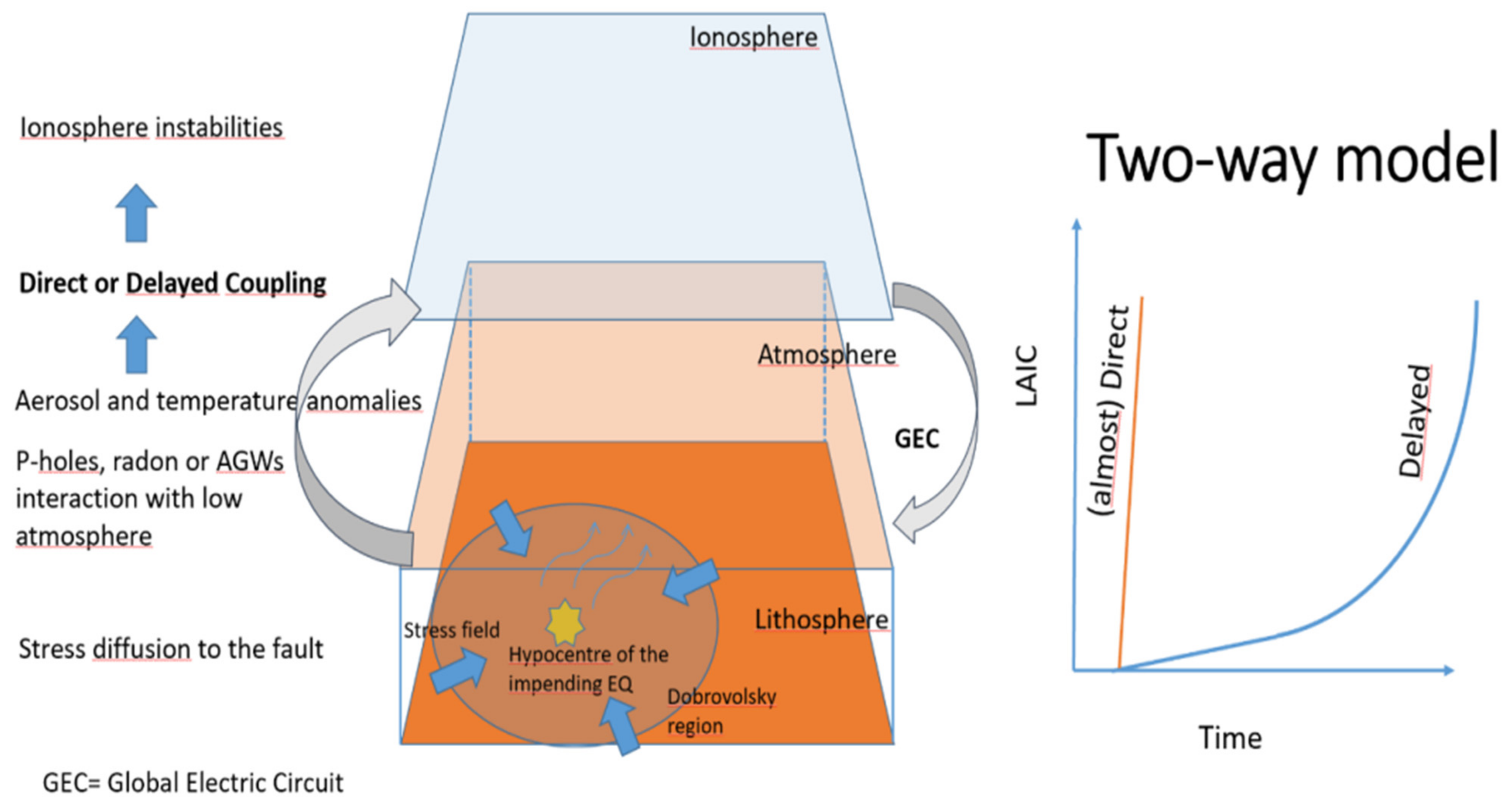
4.2. The Coupling Process of Lithosphere–Atmosphere–Ionosphere

On the basis of the multi-parameter analysis, a few long-term precursors have been exhibited in the lithosphere, such as in the b-value, R-AMR, or Earth resistivity, with anomalies starting more than 1 year or even 2 years before. For EM signals from ground-based and space-borne observations or parameters in the atmosphere, the time period of 90 days prior to the Luding earthquake has been studied, and all the anomalies are summarized in Table S1, in which the ELF magnetic field and AEF also showed continuous anomalies and enhanced at some time segments. To illustrate the relationship among different parameters, we focused on the last 3 months before the earthquake, and collected and plotted the individual abnormal signals in Figure 20, drawing them from bottom to top as they come from the atmosphere to the ionosphere. It can be seen that from the top energetic particles from NOAA and CSES, the anomalies concentrated around 10 days and 2–4 days before, then for other parameters onboard CSES, two time intervals found with −50~−60 days and −10~−15 days, for Swarm satellites one part occurred around −60~−90 days and one −10~−15 days, for TEC only −10~−15 days confirmed with Luding earthquake, as while in ionosonde two anomalies being consistent with two intervals of CSES, and the bottom ones in atmosphere are also mainly at −50~−60 days and −10~−25 days. The anomalies in the ionosphere are much greater than those in the atmosphere, which illustrates at least two ways in the LAIC process, one from the lithosphere, through the atmosphere to the ionosphere (“thermodynamic” or “diffusive-delayed” coupling), and one directly from the lithosphere to the ionosphere (“direct” coupling). The former one may correspond to the chemical channel or acoustic gravity channel in the model of Hayakawa (2004), and the latter one is likely related to the EM coupling channel, which does not practically interact with the atmosphere.

As an illuminating example, we take into consideration the day of 24 August (i.e., 12 days before the mainshock), when a lot of disturbances were detected, to demonstrate the coupling processes from the lithosphere to the atmosphere and ionosphere. Six out of eight ground-based ELF magnetometers in Sichuan Province showed significant disturbances (Figure 21a), and more than 10 AEF stations, which are mainly located near the epicenter and along the Longmenshan and Anninghe faults (Figure 21c), exhibited electric field decreases. Compared with the SKT anomaly (Figure 21d), which mainly concentrated at the east region of the epicenter, the atmospheric electric field anomalies were mainly produced along the boundary faults (Figure 21c), so not spatially coinciding with the anomalous region of SKT. Regarding the ionosphere, the GIM TEC anomaly was located south of the epicenter with its conjugate region near Indonesia (Figure 21e), which may have moved in the southern direction along the magnetic field line when the electric field coupled into the ionosphere to induce the TEC perturbations, which is consistent with the coupling process of the chemical channel, also called the overlapped electric field channel. Regarding the CSES magnetic field (Figure 21f), the X and Z disturbances were just over the epicenter, along an orbit east of the Luding earthquake, without shifting to the south, as shown by TEC. The geomagnetic field ULF ground data at Xichang station (102.5°E, 27.9°N) were processed, and their wavelet spectrum showed an enhancement at the frequency band of 0.001–0.005 Hz during 23–24 August, especially at the beginning and end hours of 24 August (Figure 21b). At the Yingjing station (Figure 21a), the ELF magnetic field curves exhibited disturbances at LT9-15 and 22-24 (i.e., UT01-07 and 14-16, respectively), basically at the same times as shown by the ULF geomagnetic field at the Xichang station. The CSES magnetic field anomaly along the orbit #252940 occurred at about UT07:25, while that of the GIM TEC appeared at UT06-08 (Figure 21e); so, the ground geomagnetic disturbance occurred 1–2 h earlier than the satellite ones, illustrating the direct coupling process from the lithosphere to the ionosphere, with some interactions with the atmosphere, possibly supporting an AGW coupling.

4.3. The Coupling Mechanisms

On the basis of what was described before, Figure 22 presents a possible LAIC model, that we call a “two-way model” because it consists of two possible modes of interaction between the different geolayers: one is almost direct, probably EM, and the other is delayed, probably based on a diffusive thermodynamic process.

In particular, in our case study, the resulting series of anomalies, mostly progressing thermodynamically from the lithosphere to the atmosphere and ionosphere, can be associated with the delayed model of coupling, and partly with EM, because directly coupling, we can associate with the almost direct model of coupling. The first anomalies appear in the lithosphere with the start of seismic acceleration and then with the anomalous decreasing b-value. Then the atmospheric anomalies appear together with some initial ionospheric anomalies that continue till the time of the earthquake occurrence. The other kind of anomalies appears sporadically, oscillating with a period that starts with 50 day and then shortens as the earthquake is approaching.

5. Conclusions

The case study of the 2022 M6.8 Luding earthquake was studied with an intensive multi-parameter and multi-layer approach composed of many parameters; this work is certainly one of the most complete in this field, for the very high number of parameters analyzed. Moreover, great care was applied to the anomaly detection in order to isolate as much as possible the potential earthquake-related anomalies from the lithospheric, atmospheric, and ionospheric data. The overall comprehensive accumulation of anomalies has two kinds of trends: one is exponential and the other is oscillating. When the ionospheric anomalies occurring before the atmospheric ones are removed, the fluctuations around the exponential cumulative number of anomalies almost disappear, confirming that those oscillations were produced by the latter kind of anomalies. Basically, the two behaviors are characteristics of two modes of LAIC processes, one of a diffusive/delayed nature (thermodynamic), and the other being a direct (electromagnetic) LAIC mechanism, with an oscillating trend.

The main outcomes from the analysis of multiple parameters before the occurrence of the Luding earthquake on 5 September 2022 are summarized as follows:

• There was a significant exponential increase in anomaly numbers detected in atmospheric and ionospheric parameters from 50 days before the Luding earthquake (i.e., −50 days); the long-term variations continued for more than 1 or 2 years in most lithospheric parameters;
• Simultaneous disturbances have been found in the ground geomagnetic field and ELF EM emissions from the lithosphere, in skin temperature and the atmospheric electric field from the atmosphere, and in the TEC and magnetic field on satellites from the ionosphere on the same day, to illustrate the direct coupling way;
• There were fewer anomalies detected in SKT compared with those electromagnetic parameters in the ionosphere and lithosphere, to demonstrate the more effective electromagnetic coupling way from the lithosphere to the ionosphere directly than the thermodynamic way with the coupling process in the atmosphere;
• The ionospheric disturbances occurred a longer time before the earthquake, more than 2 months, being consistent with the statistical results for strong earthquakes, and the analysis on multiple parameters showed a significant contribution to further the limit for the impending time of the EQ.

References

1. Hayakawa, M. Electromagnetic phenomena associated with earthquakes: A frontier in terrestrial electromagnetic noise environment. Recent Res. Dev. Geophys. 2004, 6, 81–112. Available online: https://www.researchgate.net/publication/291796289_Electromagnetic_phenomena_associated_with_earthquakes_A_frontier_in_terrestrial_electromagnetic_noise_environment#fullTextFileContent (accessed on 1 January 2004).
2. Pulinets, S.; Ouzounov, D. Lithosphere-Atmosphere-Ionosphere Coupling (LAIC) model: An unified concept for earthquake precursors validation. J. Asian Earth Sci. 2011, 41, 371–382. [Google Scholar] [CrossRef]
3. Kuo, C.L.; Huba, J.D.; Joyce, G.; Lee, L.C. Ionosphere plasma bubbles and density variations induced by pre-earthquake rock currents and associated surface charges. J. Geophys. Res. Space Phys. 2011, 116, A10317. [Google Scholar] [CrossRef]
4. Kuo, C.L.; Lee, L.C.; Huba, J.D. An improved coupling model for the lithosphere-atmosphere-ionosphere system. J. Geophys. Res. Space Phys. 2014, 119, 3189–3205. [Google Scholar] [CrossRef]
5. Zhou, C.; Liu, Y.; Zhao, S.F.; Liu, J.; Zhang, X.; Huang, J.P.; Shen, X.H.; Ni, B.; Zhao, Z.Y. An electric field penetration model for seismo-ionospheric research. Adv. Space Res. 2017, 60, 2217–2232. [Google Scholar] [CrossRef]
6. Carbone, V.; Piersanti, M.; Materassi, M.; Battiston, R.; Lepreti, F.; Ubertini, P. A mathematical model of lithosphere-atmosphere coupling for seismic events. Sci. Rep. 2021, 11, 8682. [Google Scholar] [CrossRef]
7. Gao, Y.X.; Li, T.; Zhou, G.; Chen, C.H.; Sun, Y.Y.; Zhang, X.; Liu, J.Y.; Wen, J.; Yao, C.; Bai, X. Acoustic-gravity waves generated by a point source on the ground in a stratified atmosphere-Earth structure. Geophys. J. Int. 2023, 232, 764–787. [Google Scholar] [CrossRef]
8. Molchanov, O.A.; Hayakawa, M.; Rafalsky, V.A. Penetration characteristics of electromagnetic emissions from an underground seismic source into the atmosphere, ionosphere, and magnetosphere. J. Geophys. Res. 1995, 100, 1691–1712. [Google Scholar] [CrossRef]
9. Bortnik, J.; Bleier, T. Full Wave Calculation of the Source Characteristics of Seismogenic Electromagnetic Signals as Observed at LEO Satellite Altitudes//American Geophysical Union. AGU 2004 Fall Meeting Abstracts. San Francisco: AGU: 2004, T51B-0453. Available online: https://ui.adsabs.harvard.edu/abs/2004AGUFM.T51B0453B/abstract (accessed on 31 December 2004).
10. Ozaki, M.; Yagitani, S.; Nagano, I.; Miyamura, K. Ionospheric penetration characteristics of ELF waves radiated from a current source in the lithosphere related to seismic activity. Radio Sci. 2009, 44, RS1005. [Google Scholar] [CrossRef]
11. Zhao, S.F.; Shen, X.H.; Liao, L.; Zeren, Z. A lithosphere-atmosphere-ionosphere coupling model for ELF electromagnetic waves radiated from seismic sources and its possibility observed by the CSES. Sci. China Technol. Sci. 2021, 64, 2551–2559. [Google Scholar] [CrossRef]
12. De Santis, A.; Cianchini, G.; Marchetti, D.; Piscini, A.; Sabbagh, D.; Perrone, L.; Campuzano, S.; Inan, S. A multiparametric approach to study the preparation phase of the 2019 M7.1 Ridgecrest (California, United States) Earthquake. Front. Earth Sci. 2020, 8, 540398. [Google Scholar] [CrossRef]
13. Xie, T.; Chen, B.; Wu, L.; Dai, W.; Kuang, C.; Miao, Z. Detecting seismo-ionospheric anomalies possibly associated with the 2019 Ridgecrest (California) earthquakes by GNSS, CSES, and Swarm observations. J. Geophys. Res. Space Phys. 2021, 126, e2020JA028761. [Google Scholar] [CrossRef]
14. De Santis, A.; Perrone, L.; Calcara, M.; Campuzano, S.A.; Cianchini, G.; D’Arcangelo, S.; Di Mauro, D.; Marchetti, D.; Nardi, A.; Orlando, M.; et al. A comprehensive multiparametric and multilayer approach to study the preparation phase of large earthquakes from ground to space: The case study of the June 15 2019, M7.2 Kermadec Islands (New Zealand) earthquake. Remote Sens. Environ. 2022, 283, 113325. [Google Scholar] [CrossRef]
15. Nie, L.; Zhang, X. Identification and Analysis of Multi-Station Atmospheric Electric Field Anomalies before the Yangbi Ms 6.4 Earthquake on 21 May 2021. Atmosphere 2023, 14, 1579. [Google Scholar] [CrossRef]
16. Wu, L.; Wang, X.; Qi, Y.; Lu, J.; Mao, W. Characteristics and mechanisms of near-surface atmospheric electric field negative anomalies preceding the 5 September, 2022, Ms6.8 Luding earthquake, China. Nat. Hazards Earth Syst. Sci. 2024, 24, 773–789. [Google Scholar] [CrossRef]
17. Yang, S.-S.; Asano, T.; Hayakawa, M. Abnormal gravity wave activity in the stratosphere prior to the 2016 Kumamoto earthquakes. J. Geophys. Res. Space Phys. 2019, 124, 1410–1425. [Google Scholar] [CrossRef]
18. Piersanti, M.; Materassi, M.; Battiston, R.; Carbone, V.; Cicone, A.; D’Angelo, G.; Diego, P.; Ubertini, P. Magnetospheric–Ionospheric–Lithospheric Coupling Model. 1: Observations during the 5 August 2018 Bayan Earthquake. Remote Sens. 2020, 12, 3299. [Google Scholar] [CrossRef]
19. Hayakawa, M.; Itoh, T.; Hattori, K.; Yumoto, K. ULF electromagnetic precursors for an earthquake at Biak, Indonesia on February 17, 1996. Geophys. Res. Lett. 2000, 27, 1531–1534. [Google Scholar] [CrossRef]
20. Harada, M.; Hattori, K.; Isezaki, N. Transfer function analysis approach for anomalous ULF geomagnetic field change detection. Phys. Chem. Earth 2004, 29, 409–417. [Google Scholar] [CrossRef]
21. Parrot, M.; Berthelier, J.J.; Lebreton, J.P.; Sauvaud, J.A.; Santolik, O.; Blecki, J. Examples of unusual ionospheric observations made by the DEMETER satellite over seismic regions. Phys. Chem. Earth 2006, 31, 486–495. [Google Scholar] [CrossRef]
22. Huang, J.; Zhang, F.; Li, Z.; Shen, X.; Yang, B.; Li, W.; Zeren, Z.; Lu, H.; Tan, Q. Disturbance identification of electric field data observed by the CSES-01 satellite before earthquakes. Sci. China Earth Sci. 2023, 66, 1814–1824. [Google Scholar] [CrossRef]
23. Li, G.; Wang, A.; Gao, Y. Source rupture characteristics of the September 5, 2022 Luding Ms 6.8 earthquake at the Xianshuihe fault zone in southwest China. Earthq. Res. Adv. 2023, 3, 100201. [Google Scholar] [CrossRef]
24. Zhang, Z.; Fang, L.H.; Xu, L.S. Primary source characteristics of the 2022 Sichuan Luding Ms6.8 Earthquake. Chin. J. Geophys. 2023, 66, 1397–1408. [Google Scholar] [CrossRef]
25. An, Y.; Wang, D.; Ma, Q.; Xu, Y.; Li, Y.; Zhang, Y.; Liu, Z.; Huang, C.; Su, J.; Li, J.; et al. Preliminary report of the September 5, 2022 Ms6.8 Luding earthquake, Sichuan, China. Earthq. Res. Adv. 2023, 3, 100184. [Google Scholar] [CrossRef]
26. Jing, F.; Jiang, M.; Zhang, L.; Singh, R.P. Detection and Identification of Preseismic Thermal Anomalies in Cloudy Conditions Associated with the 2022 Luding (China) Mw 6.6 Earthquake. IEEE Trans. Geosci. Remote Sens. 2023, 61, 4104612. [Google Scholar] [CrossRef]
27. Lu, C.; Zhou, X.; Chen, Z.; Liu, Z.; Hu, L.; Sun, F.; Martinelli, G.; Ying, L. Earthquake geochemical scientific expedition and research. Earthq. Res. Adv. 2023, 3, 100239. [Google Scholar] [CrossRef]
28. Chen, C.-H.; Zhang, S.; Mao, Z.; Sun, Y.-Y.; Liu, J.; Chen, T.; Zhang, X.; Yisimayili, A.; Qing, H.; Luo, T.; et al. The Lithosphere-Atmosphere-Ionosphere Coupling of Multiple Geophysical Parameters Approximately 3 Hours Prior to the 2022 M6.8 Luding Earthquake. Geosciences 2023, 13, 356. [Google Scholar] [CrossRef]
29. Dobrovolsky, I.P.; Zubkov, S.I.; Miachkin, V.I. Estimation of the size of earthquake preparation zones. Pure Appl. Geophys. 1979, 117, 1025. [Google Scholar] [CrossRef]
30. De Santis, A.; Cianchini, G.; Di Giovambattista, R. Accelerating moment release revisited: Examples of application to Italian seismic sequences. Tectonophysics 2015, 639, 82–98. [Google Scholar] [CrossRef]
31. Lu, J.; Xie, T.; Li, M.; Wang, Y.L.; Ren, Y.X.; Gao, S.D.; Wang, L.W.; Zhao, J.L. Monitoring shallow resistivity changes prior to the 12 May 2008 M 8.0 Wenchuan earthquake on the Longmenshan tectonic zone. China. Tectonophysics 2016, 675, 244–257. [Google Scholar] [CrossRef]
32. Hattori, K.; Serita, A.; Yoshino, C.; Hayakawa, M.; Isezaki, N. Singular spectral analysis and principal component analysis for signal discrimination of ULF geomagnetic data associated with 2000 Izu Island Earthquake Swarm. Phys. Chem. Earth 2006, 31, 281–291. [Google Scholar] [CrossRef]
33. Cianchini, G.; De Santis, A.; Di Giovambattista, R.; Abbattista, C.; Amoruso, L.; Campuzano, S.A.; Carbone, M.; Cesaroni, C.; De Santis, A.; Marchetti, D.; et al. Revised Accelerated Moment Release Under Test: Fourteen Worldwide Real Case Studies in 2014–2018 and Simulations. Pure Appl. Geophys. 2020, 177, 4057–4087. [Google Scholar] [CrossRef]
34. Hayakawa, M.; Izutsu, J.; Yu Schekotov, A.; Nickolaenko, A.P.; Galuk, Y.; Kudintseva, I.G. Anomalies of Schumann resonances as observed near Nagoya associated with two huge (M~7) Tohoku offshore earthquakes in 2021. J. Atmos. Solar-Terr. Phys. 2021, 225, 105761. [Google Scholar] [CrossRef]
35. Schekotov, A.Y.; Molchanov, O.A.; Hayakawa, M.; Fedorov, E.N.; Chebrov, V.N.; Sinitsin, V.I.; Yagova, N.V. ULF/ELF magnetic field variations from atmosphere induced by seismicity. Radio Sci. 2007, 42, RS6S90. [Google Scholar] [CrossRef]
36. Piscini, A.; De Santis, A.; Marchetti, D.; Cianchini, G. A New Multi-Parametric Climatological Approach to the Study of the Earthquake Preparatory Phase: The 2016 Amatrice-Norcia (Central Italy) Seismic Sequence. In: EGU 2017. EGU2017-14105. Available online: https://ui.adsabs.harvard.edu/abs/2017EGUGA..1914105P/abstract (accessed on 30 April 2017).
37. Le, H.; Liu, L.Y.; Liu, L. A statistical analysis of ionospheric anomalies before 736 M6.0+ earthquakes during 2002–2010. J. Geophys. Res. 2011, 116, A02303. [Google Scholar] [CrossRef]
38. Shen, X.H.; Zong, Q.-G.; Zhang, X.M. Introduction to special section on the China Seismo-Electromagnetic Satelliteand initial results. Earth Planet. Phys. 2018, 2, 439–443. [Google Scholar] [CrossRef]
39. De Santis, A.; Marchetti, D.; Pavón-Carrasco, F.J.; Cianchini, G.; Perrone, L.; Abbattista, C.; Alfonsi, L.; Amoruso, L.; Campuzano, S.A.; Carbone, M.; et al. Precursory worldwide signatures of earthquake occurrences on Swarm satellite data. Sci. Rep. 2019, 9, 20287. [Google Scholar] [CrossRef]
40. Evans, D.S.; Greer, M.S. Polar Orbiting Environmental Satellite Space Environment Monitor—2 Instrument Descriptions and Archive Data Documentation, Natl. Atmos. and Oceanic Admin., Space Environ. Cent, Boulder, Colorado, NOAA Technical Memorandum OAR SEC 93, Version 1.4. 2004. Available online: https://ngdc.noaa.gov/stp/satellite/poes/docs/SEM2Archive.pdf (accessed on 14 April 2010).
41. Fidani, C. West Pacific Earthquake Forecasting Using NOAA Electron Bursts With Independent L-Shells and Ground-Based Magnetic Correlations. Front. Earth Sci. 2021, 9, 673105. [Google Scholar] [CrossRef]
42. Gutenberg, B.; Richter, C.F. Frequency of earthquakes in California. Bull. Seism. Soc. Am. 1944, 34, 185–188. [Google Scholar] [CrossRef]
43. Wiemer, S.; Wyss, M. Mapping the frequency–magnitude distribution in asperities: An improved technique to calculate recurrence times? J. Geophys. Res. 1997, 102, 15115–15128. [Google Scholar] [CrossRef]
44. Schorlemmer, D.; Wiemer, S.; Wyss, M. Variations in earthquake-size distribution across different stress regimes. Nature 2005, 437, 539–542. [Google Scholar] [CrossRef]
45. Scholz, C.H. On the stress dependence of the earthquake b value. Geophys. Res. Lett. 2015, 42, 1399–1402. [Google Scholar] [CrossRef]
46. Nuannin, P.; Kulhanek, O.; Persson, L. Spatial and temporal b value anomalies preceding the devastatingoff coast of NW Sumatra earthquake of December 26, 2004. Geophys. Res. Lett. 2005, 32, L11307. [Google Scholar] [CrossRef]
47. Schorlemmer, D.; Wiemer, S. Microseismicity data forecast rupture area. Nature 2005, 434, 1086. [Google Scholar] [CrossRef]
48. Taroni, M.; Vocalelli, G.; De Polis, A. Gutenberg–Richter B-value time series forecasting: A weighted likelihood approach. Forecasting 2021, 3, 561–569. [Google Scholar] [CrossRef]
49. Wang, R.; Chang, Y.; Miao, M.; Zeng, Z.; Chen, H.; Shi, H.; Li, D.; Liu, L.; Su, Y.; Han, P. Assessing Earthquake Forecast Performance Based on b Value in Yunnan Province, China. Entropy 2021, 23, 730. [Google Scholar] [CrossRef]
50. Wiemer, S.; Wyss, M. Minimum Magnitude of Completeness in Earthquake Catalogs: Examples from Alaska, the Western United States and Japan. Bull. Seismol. Am. 2000, 90, 859–869. [Google Scholar] [CrossRef]
51. Bowman, D.D.; Ouillon, G.; Sammis, C.G.; Sornette, A.; Sornette, D. An observational test of the critical earthquake concept. J. Geophys. Res. 1998, 103, 24359–24372. [Google Scholar] [CrossRef]
52. Jaumé, S.; Sykes, L.R. Evolving towards a critical point: A review of accelerating seismic moment/energy release prior to large and great earthquakes. Pure Appl. Geophys. 1999, 155, 279. [Google Scholar] [CrossRef]
53. Cianchini, G.; De Santis, A.; Barraclough, D.R.; Wu, L.X.; Qin, K. Magnetic transfer function entropy and the 2009 Mw = 6.3 L’Aquila earthquake (Central Italy). Nonlin. Process. Geophys. 2012, 19, 401–409. [Google Scholar] [CrossRef]
54. Bufe, C.G.; Varnes, D.J. Predictive modeling of the seismic cycle of the Greater San Francisco Bay Region. J. Geophys. Res. 1993, 98, 9871–9883. [Google Scholar] [CrossRef]
55. Wells, D.L.; Coppersmith, K.J. New Empirical Relationships among Magnitude, Rupture Length, Rupture Width, Rupture Area, and Surface Displacement. Bull. Seismol. Am. 1994, 84, 974–1002. [Google Scholar] [CrossRef]
56. Xie, T.; Han, Y.; Ye, Q.; Xue, Y. Changes and mechanisms of apparent resistivity before earthquakes of MS6.0–6.9 on the Chinese mainland. Front. Earth Sci. 2023, 11, 1187660. [Google Scholar] [CrossRef]
57. Korsunova, L.P.; Khegai, V.V. Analysis of seismo-ionospheric disturbances at the chain of Japanese stations for vertical sounding of the ionosphere. Geomagn. Aeron. 2008, 48, 392–399. [Google Scholar] [CrossRef]
58. Perrone, L.; De Santis, A.; Abbattista, C.; Alfonsi, L.; Amoruso, L.; Carbone, M.; Cesaroni, C.; Cianchini, G.; De Franceschi, G.; De Santis, A.; et al. Ionospheric Anomalies Detected by Ionosonde and Possibly Related to Crustal Earthquakes in Greece. Ann. Geophys. 2018, 36, 361–371. [Google Scholar] [CrossRef]
59. Kim, V.P.; Khegai, V.V.; Illich-Svitych, P.V. Probability of formation of a metallic ion layer in the nighttime mid-latitude ionospheric E-region before strong earthquakes. Geomagn. Aeron. 1993, 33, 114–119. (In Russian) [Google Scholar]
60. Kim, V.P.; Khegai, V.V.; Illich-Svitych, P.V. On one possible ionospheric precursor of earthquakes. Phys. Solid Earth 1994, 30, 223–226. (In Russian) [Google Scholar]
Figure 1. Temporal variation in the b-value from 1 January 2012 to 28 October 2023. The continuous vertical red bar identifies the day on which the Luding earthquake occurred; the dashed red bar marks the beginning of the b-value decrease.
Remotesensing 16 02381 g001
Figure 2. R-AMR algorithm applied to the seismic catalogue. The red curve and the black line are, respectively, the power-law and linear fits of s(t). The vertical dashed green line is the origin time of the mainshock. The lower inset is the time distribution of the catalogue contributing to acceleration: the red dots are the events occurring within the inner circle with R0 = 33 km radius, representing the fault area; the green dots are the events outside the inner circle, i.e., those occurring in the external damped region (circular annulus with R1 = 140 km radius).
Remotesensing 16 02381 g002
Figure 3. The spatial distribution of the seismic events which contributed to the acceleration found by the R-AMR method. The fault is modeled as a circular area with a radius equal to the theoretical length of the rupture, which scales with the magnitude—33 km in this case according to Wells and Coppersmith (1994) [55]. Differently from the events represented by the red dots, all the events (blue) are those events with a damping function of the distance from the fault.
Remotesensing 16 02381 g003
Figure 4. The Earth resistivity observations at four stations around Luding earthquake during 2018–2022 ((a,b) for Ganzi station; (c,d) for Jiangyou; (e,f) for Mianning; (g,h) for Hongge station; the epicentral distances were marked in brackets below the earthquake’s name and magnitude with red vertical arrows; the red lines indicate the long-term trend and double directional red arrows present the duration for annual variation).
Remotesensing 16 02381 g004
Figure 5. The comparison of resistivity (red line) and precipitation (blue histogram) in 2022 at 3 stations (yellow rectangle marks the quick decrease during March and April).
Remotesensing 16 02381 g005
Figure 6. The series of ELF magnetic field abnormal signals at 8 stations around Luding earthquake from 1 May to 13 September 2022 (three earthquakes are marked as Lushan on 1 June, Maerkang on 10 June, and Luding on 5 September with vertical red dotted lines; black lines indicate the increase trend at different time period).
Remotesensing 16 02381 g006
Figure 7. The AEF observations at multiple stations ((ae) AEF curves at Yanzigou, Caoke, Xinglong, Guzan, Ya’an) and related meteorological factors ((f) precipitation; (g) visibility, the dotted blue line indicates its threshold, which means that when the values are lower than it, the AEF observations will be affected by this factor, so it cannot be defined as an anomaly related to earthquakes; (h) the maximum wind speed with its threshold by red dotted line where this factor cannot exceed it; (i) humidity with threshold by red dotted line where this dactor cannot exceed it) in Luding on 15 August 2022 (the yellow colors point out the AEF anomalies and the time period with the green color may be related to strong wind with wind speed greater than 8 m/s).
Remotesensing 16 02381 g007
Figure 8. The statistical analysis on the stations with AEF anomalies from 1 August to 5 September 2022. (a) The occurrence date of anomalies at each station with the distance to the epicenter (the blue square represent the anomalies occurred at each station); (b) the total number of abnormal stations with blue columns on each day; (c) the percentage of stations with AEF anomalies to the total studied ones. In (b,c) the horizontal dashed lines indicate the levels of 1 or 2 standard deviations.
Remotesensing 16 02381 g008
Figure 9. Analysis of the SKT and OLR parameters for Luding Ms6.8 earthquake with comparison between the 2022 time series (dashed red line) and the historical time series (1980–2021, blue line). Each red oval puts in evidence the identified anomalies that are characterized by a 2-day nighttime persistence with values surpassing two standard deviations with respect to the historical mean. Colored stripes indicate 1.0 σ (light green), 1.5 σ (green), and 2.0 σ (yellow) from the mean of the historical time series, respectively (please note that in the legend of the figures on the left, “std” means standard deviation σ, therefore “1*std”, “1.5*std” and “2*std” stand for “1.0 σ”, “1.5 σ” and “2.0 σ”, respectively). The earthquake occurred at the end of the analyzed period (red vertical line). On the right, the corresponding anomalous day spatial maps are depicted (the one on 24 August for SKT and on 7 July 2022 for OLR). The epicenter is indicated by a star in the center of the map; as background, the system of faults is shown with grey lines.
Remotesensing 16 02381 g009
Figure 10. The GPS TEC time series analysis during 22–28 August 2022 ((a) the red rectangle indicates the anomaly in TEC on 26 August) and the spatial distribution of T E C in China on 26 August 2022 (b).
Remotesensing 16 02381 g010
Figure 11. The GIM TEC at UT06-10 during 24 and 26 August 2022 ((a) the epicenter has a red star, and the conjugate has a blue star, where one is Luding earthquake at northern hemisphere, and one is Indonesian earthquake at southern hemisphere) and the T E C from 1 July to 11 September 2022 at longitude scale of 100–105°E ((b) the earthquakes occurring at the conjugate regions were all marked with related information; gray color illustrates the days affected by solar or geomagnetic activities).
Remotesensing 16 02381 g011
Figure 12. The distribution of Ne observed by CSES in the daytime on 23 August 2022. The panels from top to bottom are as follows: the Ne observation, the 15-day background, and the relative change, respectively. The red and blue stars represent the epicenter and its conjugate point, respectively.
Remotesensing 16 02381 g012
Figure 13. The anomalies in the three components of geomagnetic field at 250 Hz (±50 Hz) from SCM onboard CSES during nighttime in 1−30 July (top) and 10 August to 9 September (bottom) 2022. At the top of each series, the magnetic indices Kp and Dst are shown. Vertical red line is the time of earthquake occurrence.
Remotesensing 16 02381 g013
Figure 14. The ionospheric anomaly on 3 July 2022 (a) and 13 July 2022 (b) using observed Δh’Es, δfoEs, and δfoF2 variations (arrows) (please note that the time is in LT).
Remotesensing 16 02381 g014
Figure 15. Swarm C (from left to right panels) first differences (MASS method for magnetic data) of X, Y, Z, F; and map with the location of the epicenter of the earthquake (green star), Dobrovolsky area (yellow circle), and analyzed track (red line) for 3 July 2022 (i.e., 64 days before the earthquake). Colored squares indicate the anomalous windows automatically detected by MASS.
Remotesensing 16 02381 g015
Figure 16. Electron CRs detected by NOAA-18 on 2 September 2022. Three electron bursts (indicated by red circles) are evidenced: two are east and one south of the earthquake’s epicentre, as indicated by a red star.
Remotesensing 16 02381 g016
Figure 17. Electron losses detected from 18 August to 11 September 2022, reported on the magnetic latitude, are indicated by green circles. Electron losses detected by CSES are indicated in yellow. Earthquake day and corresponding magnetic latitude are indicated by a red star.
Remotesensing 16 02381 g017
Figure 18. Extended electron losses detected on 2 September 2022 by CSES are reported on the geographic latitudes and longitudes. Electron fluxes are represented in different colors depending on the direction of the telescopes. The electron fluxes detected east of the Luding epicenter (red star) from telescope 9 are in brown. The earthquake epicenter is indicated by a red star.
Remotesensing 16 02381 g018
Figure 19. (a) Cumulative number of anomalies and their progression in time from about 300 days to the occurrence of the earthquake. An exponential fit (red line) is also shown. In the small insert, the curve and the fit are shown for the largest interval of time. The curve is characterized by the exponential trend together with some fluctuations. (b) As in (a) but removing those ionospheric anomalies appearing before the atmospheric ones. Almost all fluctuations, appearing in (a), disappear.
Remotesensing 16 02381 g019
Figure 20. The temporal development of different parameters from atmosphere (bottom of figure) to ionosphere (top of figure) within 90 days before Luding earthquake.
Remotesensing 16 02381 g020
Figure 21. The coupling process among lithosphere–atmosphere–ionosphere on 24 August through different parameters (In (c): red circle is the Luding epicenter; red stars are AEF stations with anomalies; green triangle is Xichang station with ULF geomagnetic observation; and blue triangle is Yingjing station with ELF magnetic observation).
Remotesensing 16 02381 g021
Figure 22. Two-way model of coupling. On the left, a sketch of the different couplings; on the right, the plot in time showing two different couplings, one direct (red) and another delayed (blue). For convenience, we indicated the former as occurring at the same time of the beginning of the delayed one, but it can appear any time after the appearance of the first lithospheric precursor.
Remotesensing 16 02381 g022