Matching Satellite Sun-Induced Chlorophyll Fluorescence to Flux Footprints Improves Its Relationship with Gross Primary Productivity

Abstract

Sun-induced chlorophyll fluorescence (SIF) holds enormous potential for accurately estimating terrestrial gross primary productivity (GPP). However, current studies often overlook the spatial representativeness of satellite SIF and GPP observations. This research downscaled TROPOMI SIF (TROPOSIF) and its enhanced product (eSIF) in China’s Saihanba Forest Region to obtain high-resolution SIF data. SIF was simulated using the SCOPE model, and the downscaled SIF’s reliability was validated at two forest eddy covariance (EC) sites (SHB1 and SHB2) in the study area. Subsequently, the downscaled SIF data were matched to the EC footprint of the two forest sites, and the relationship between SIF and GPP was compared at various observational scales. Additionally, the ability of downscaled TROPOSIF and eSIF to track GPP was compared, along with the correlations among several vegetation indices (VIs) and GPP. The findings reveal the following: (1) Downscaled TROPOSIF and eSIF showed a strong linear relationship with SCOPE-modeled SIF (R² ≥ 0.86). The eSIF closely matched the SCOPE simulation (RMSE: 0.06 mw m⁻² nm⁻¹ sr⁻¹) and displayed a more consistent seasonal variation pattern with GPP. (2) Comparisons among coarse-resolution SIF, EC footprint-averaged SIF (SIF_ECA), and EC footprint-weighted SIF (SIF_ECW) demonstrated significant improvements in the linear relationship between downscaled SIF and GPP (the R² increased from the range of 0.47–0.65 to 0.78–0.85). SIF_ECW exhibited the strongest relationship with GPP, indicating that matching SIF to flux footprints improves their relationship. (3) As the distance from the flux tower increased, the relationship between SIF and GPP weakened, reaching its lowest point beyond 1 km from the tower. Moreover, in the highly heterogeneous landscape of the SHB2 site, the relationship between VIs and GPP was poor, with no clear pattern as distance from the flux tower increased. In conclusion, the strong spatial dependency of SIF and tower-based GPP emphasizes the importance of using high-resolution SIF to accurately quantify their relationship.

1. Introduction

Sun-induced chlorophyll fluorescence (SIF) serves as a valuable byproduct of photosynthesis and has found extensive use in the investigation of processes related to photosynthesis [1,2,3,4]. In recent years, emerging SIF measurement techniques implemented on remote sensing platforms have significantly facilitated the expanded global-scale measurement of SIF, providing a promising prospect for quantifying global gross primary productivity (GPP) based on SIF. Researchers have conducted extensive investigations into satellite SIF and GPP across diverse biomes, indicating a linear relationship between them at larger regional and seasonal scales [5,6]. Several studies have utilized satellite SIF to estimate GPP at regional and global scales based on this relationship [7,8,9]. However, recent research has shed light on the presence of nonlinear SIF-GPP relationships at finer spatial and temporal scales, as well as in the presence of stressful conditions [10,11,12]. To gain further insights into the SIF-GPP relationship, researchers have examined finer scales, such as modeling the process from the photosystem emission of chlorophyll fluorescence to the sensor reception signal [1,3], as well as studying hydrothermal stress [13,14], herbicide treatment [15], etc. While extensive research has been conducted on the correlation between satellite-obtained SIF and GPP at multiple scales, limited focus has been placed on investigating the influence of the spatial extent of SIF derived from satellites and GPP obtained from eddy covariance (EC) flux towers on their interrelationship.

EC flux data have been widely used to evaluate or calibrate carbon flux and its related products from remote sensing methods, as they can provide relatively accurate GPP information. However, challenges arise when estimating GPP using EC flux tower and satellite data due to inconsistencies in the satellite data resolution and the footprint range of EC flux observations [16,17,18]. This is mainly because the current SIF products rely on medium- or coarse-resolution satellite datasets, whose spatial extents often have difficulty matching the footprint coverage area of the EC flux. In addition, the footprint coverage area and location of the EC flux vary widely over time due to changes in surface roughness and meteorological elements like wind speed and direction, especially on seasonal scales [18,19]. To address this limitation, some studies have screened larger areas with homogeneous subsurface landscapes to minimize the impact of spatial heterogeneity on GPP estimates from SIF obtained from satellite data [8,20]. However, truly homogeneous sites are rare [17], which may constrain the richness and diversity of ecosystem sample selection. Moreover, it may not be reasonable to assume spatial homogeneity of the GPP within the footprint of the EC flux, even when the land cover remains consistent within the footprint [18]. This is especially true for SIF, which is more sensitive to photosynthesis and whose spatial distribution is affected not only by plant physiology but also by canopy structure factors, including the leaf area index (LAI), clumping, and leaf angle distribution [21,22]. Therefore, spatial-scale mismatches are likely to distort the relationship between SIF and GPP.

Several reconstructed SIF products, such as Contiguous SIF (CSIF) [23], Global OCO-2 SIF (GOSIF) [24], SIFnet [25], reconstructed TROPOMI SIF (RTSIF) [26], and enhanced SIF (eSIF) [27], have been developed to overcome the limitations of the current satellite-based SIF products, such as their low spatial and temporal resolution, high noise, and spatial discontinuity. Despite the widespread use of these SIF products globally or in large regional areas, their accuracy in matching GPP data derived from EC flux towers remains limited. Therefore, obtaining high-resolution SIF data is imperative for studying the relationship between satellite SIF and tower-based GPP.

The Copernicus Sentinel-5P mission launched in October 2017 with the Tropospheric Monitoring Instrument (TROPOMI). Possessing higher spatiotemporal resolution, it provides daily global continuous spatial sampling with a minimum pixel size of 3.5 × 7.5 km² (reduced to 3.5 × 5.5 km² since August 2019), nearly covering the entire globe on a daily basis, and surpassing previous satellite-based SIF products [28,29]. However, the SIF products derived from these data amplify instantaneous SIF data under clear-sky conditions to daily averages by considering variations in the solar zenith angle, thereby neglecting the influence of weather variations on SIF. The recently introduced eSIF product addresses this limitation by accounting for all weather variations, improving upon the TROPOMI SIF product [27]. Nevertheless, these data do not represent raw SIF data, and the data reconstruction process may lead to the loss of true values. Therefore, in this study, to obtain more accurate, high-resolution SIF data, both the original TROPOMI SIF product and the eSIF product were simultaneously considered. Machine learning algorithms were used to downscale and generate high-resolution SIF products (0.0005°) and investigate the relationship between SIF products of different resolutions and GPP data derived from EC flux towers. The objectives of this study were (1) to produce high-resolution SIF products suitable for tracking seasonal changes in GPP; (2) to compare whether matching SIF with flux footprints enhances the correlation between SIF and GPP; and (3) to assess the relationship between SIF and GPP at different observational scales.

2. Materials and Methods

2.1. Study Area and In Situ Survey

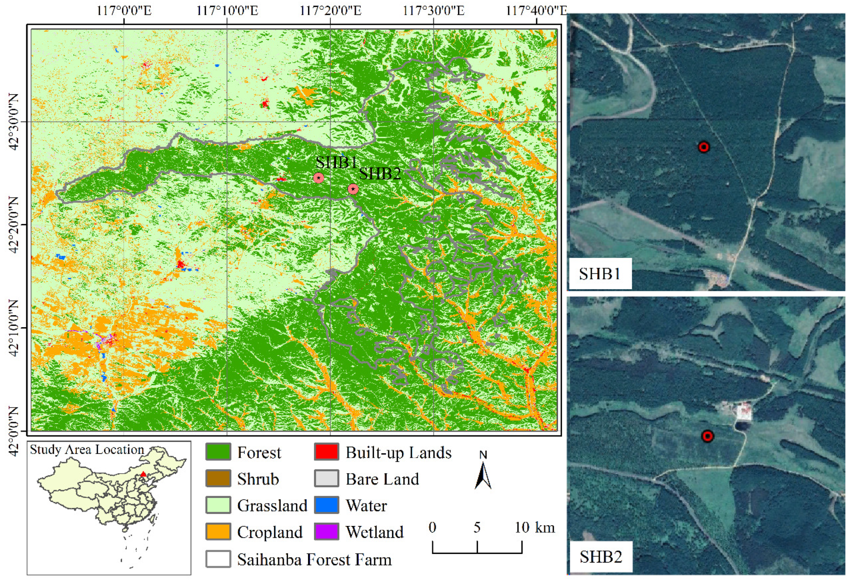
2.1.1. Study Sites

In this study, GPP was measured at two forest observation stations located in the Saihanba Forest Farm in Chengde, Hebei Province, China (Figure 1). The first station (SHB1) is located in a larch (Larix principis-rupprechtii Mayr) forest (117°18′52.61″E, 42°24′35″N), which is an artificial forest that is approximately 60 years old, with a tree height of approximately 22 m. The forest is composed of a single tree species with a high canopy density and sparse shrubs and grasses. As the land cover type is larch, the monitored larch at this observation site is highly representative. The second station (SHB2) is located in a Scots pine (Pinus sylvestris var. mongolica) forest (117°22′12″E, 42°23′28″N), which is also an artificial forest but approximately 10 years old. The forest is composed of a single species with high understory herb coverage. The canopy height of Scots pine ranges from 3 to 5 m, and the forest area is relatively small (250 m × 500 m). The area around the Scots pine forest includes grasslands, larch, and birch (Betula platyphylla) forests, making the underlying surface of the EC flux footprint relatively complex. Saihanba experiences a temperate continental monsoon climate within a cold and semiarid zone, characterized by an average temperature of −1.2 °C and an annual precipitation of 452 mm. The predominant soil type in the area is sandy loam [30].

2.1.2. Eddy Covariance and Meteorological Data Measurement

The open circuit eddy correlation system (OPEC) was installed on flux towers in both SHB1 and SHB2, at heights of 30 m and 15 m, respectively. This system monitored long-term, continuous half-hour averages of turbulence and energy flux, including latent heat (LE), sensible heat (H), and CO₂ flux. The system was equipped with a three-dimensional acoustic wave anemometer (Gill WindMaster, Gill Instruments, Lymington, Hampshire, UK) and an infrared gas analyzer (Li-7500DS, LI-COR Inc., Lincoln, NE, USA).

Meteorological data were recorded every half hour simultaneously with the flux data. A four-component radiometer (Kipp & Zonen CNR4, Delft, The Netherlands) and a photosynthetically active radiation sensor (LI-190R, Campbell Scientific, Lincoln, NE, USA) were positioned at a height of 38 m to monitor the radiation flux. At a height of 30 m, an air temperature and humidity sensor (HMP155, Vaisala, Helsinki, Finland) and a rain barrel were installed. Sensors were placed at soil depths of 5 cm, 10 cm, and 20 cm to monitor the soil temperature (TM-L20, DYNAMAX Inc., Elkhart, IN, USA) and soil water content (EC-5, METER Inc., Pullman, WA, USA). Three heat flux panels (HFP01, HukseFlux Inc., Delft, The Netherlands) were placed at a soil depth of 5 cm to measure the soil heat flux, and the meteorological data were recorded at a frequency of 0.5 Hz. A CR1000X data logger (Campbell Scientific Inc., Logan, UT, USA) recorded 30 min averages of the above variables.

The raw EC data were processed using EddyPro 7 (LI-COR Bioscience, Lincoln, NE, USA) to obtain half-hourly fluxes, which involved detecting spikes, correcting time lags and frequency responses, rotating coordinates along three axes, correcting for acoustic virtual temperature and density fluctuations, and calculating fluxes [31]. The EC data were calculated every 30 min with three different quality control levels (0, 1, and 2). Poor-quality flux data were excluded (marker 2). Unreasonable flux data were rejected by discarding flux data collected half an hour before and up to one hour after precipitation, excluding observations obtained during instrument failures or atmospheric instability conditions, eliminating negative CO₂ flux values observed at night, and rejecting flux values that fell outside of the acceptable range. For gap filling and flux partitioning, the REddyProc online tool was utilized [32]. The daytime-based separation method was used to divide the NEE into ecosystem respiration (Re) and GPP components at 30 min intervals [33].

2.2. Remote Sensing Data

2.2.1. Sentinel-2 Data

The 2020–2021 Sentinel-2A/B Multispectral Instrument (MSI) surface reflectance (SR) data (Level-2A) were utilized to obtain the vegetation indices (VIs) in the Saihanba region. Sentinel-2 offers high-resolution Earth imagery (10–60 m resolution in all bands) and has a revisiting period of 5 days. The sensor on board the Sentinel-2 satellites consists of 13 channels, encompassing the visible spectrum, the near-infrared (NIR), and shortwave infrared (SWIR) bands. The Google Earth Engine (GEE) platform was utilized to process the Sentinel-2 data. Cloud and shadow masks were first applied to the Sentinel-2 dataset to extract cloud-free and shadow-free data. The cloud-masking algorithm devised by the Sentinel Hub [34] was utilized to identify clouds within the Sentinel-2 cloud probability dataset (s2cloudless), and shadows were determined as the intersections of cloud projections and low-reflection near-infrared (NIR) pixels. However, the algorithm did not completely eliminate clouds and shadows in the Saihanba area, so the QA60 bitmask band provided by the European Space Agency (ESA) in the metadata was additionally used to effectively remove clouds and cirrus. Furthermore, cloud shadows were eliminated using solar geometry and height estimates [35]. During the masking process, the results were visually inspected, and all parameters were adjusted until the best results were obtained. To generate an 8-day composite, the mean synthesis of valid Sentinel-2 VIs was used. Data gaps were then filled using linear interpolation to achieve complete coverage over the entire 8-day period. The resulting time series was smoothed using a Savitzky–Golay (SG) filter with a third-order polynomial and a window size of 56 days (7 observations), as described by You et al. [36]. Finally, a consistent 8-day Sentinel-2 time series that was free of clouds and effectively filled in data gaps was acquired (refer to Figure 2).

This study utilized six spectral VIs obtained from Sentinel-2 SR data, namely the enhanced vegetation index (EVI), near-infrared reflectance of terrestrial vegetation (NIRv), red-edge normalized difference vegetation index (NDVIre), chlorophyll index—red (CIr), chlorophyll sensitive index (CSI), and terrestrial chlorophyll index (MTCI). These indices were computed using bands B3 to B8, with central wavelengths of 560 nm, 665 nm, 705 nm, 740 nm, 783 nm, and 842 nm, respectively. The calculation formulas for each index can be found in

Table 1. The vegetation indices used in this study.

VI Name	Formula	Reference
CIr	$\frac{\mathrm{B}7}{\mathrm{B}5}-1$	Gitelson et al. [37]
MTCI	$\frac{\mathrm{B}6-\mathrm{B}5}{\mathrm{B}5-\mathrm{B}4}$	Dash and Curran [38]
CSI	$2.5\ast \frac{\mathrm{B}8-\mathrm{B}5}{\mathrm{B}8 + \mathrm{B}5}\ast \frac{\mathrm{B}2}{\mathrm{B}5}$	Zhang et al. [39]
EVI	$2.5\ast \frac{\mathrm{B}8-\mathrm{B}4}{\mathrm{B}8 + 6 \ast \mathrm{B}4-7.5 \ast \mathrm{B}2 + 1}$	Huete et al. [40]
NDVIre	$\frac{\mathrm{B}8-\mathrm{B}5}{\mathrm{B}8 + \mathrm{B}5}$	Sims and Gamon [41]
NIRv	$\frac{\mathrm{B}8-\mathrm{B}4}{\mathrm{B}8 + \mathrm{B}4}\times \mathrm{B}4$	Badgley et al. [42]

. All VIs resolutions were resampled to 0.0005° for subsequent SIF downscaling.

2.2.2. SIF Data

TROPOSIF refers to the satellite-based SIF product retrieved from the TROPOMI spectrometer on board the Sentinel-5 Precursor satellite [29]. It provides ungridded Level-2B daily aggregated data, where daily aggregation is achieved by scaling the TROPOMI observations (local solar time 13:30) with daily length scale factors [29]. The SIF retrieval employs a data-driven approach based on principal component analysis and is applied within two fitting windows (743–758 and 735–758 nm). Due to its robustness against atmospheric influences compared to the 735–758 nm SIF [29], the 743–758 nm daily average SIF product was exclusively utilized, filtering out observations with cloud fractions exceeding 0.2 and viewing zenith angles exceeding 60° and solar zenith angles exceeding 70°. TROPOSIF data were aggregated into 0.05° grid cells every 8 days.

The eSIF data, created by Liu et al. [27], provide global SIF data with an 8-day temporal resolution and a spatial resolution of 0.05°. They combine TROPOSIF data with information on the near-infrared radiation reflected by vegetation (NIRvP). Notably, the eSIF data demonstrate reduced angular dependence and an improved signal-to-noise ratio compared to the original TROPOSIF data. As a result, the eSIF data are better equipped for capturing seasonal variations in GPP under environmental stress conditions [27].

2.2.3. LAI and Photosynthetically Active Radiation (PAR) Data

LAI and PAR were utilized for downscaling purposes, with LAI serving as an indicator of vegetation structural distribution while PAR delineates the spatial distribution of photosynthetically available radiation. The LAI data employed originate from the Global Land Surface Satellite (GLASS) series [43], with a temporal resolution of 8 days. Among the available spatial resolutions for LAI products, the finest resolution of 250 m was selected. The PAR data were derived from the Breathing Earth System Simulator (BESS) PAR product [44], with a temporal daily resolution and a spatial resolution of 0.05°, aggregating every 8 days.

2.3. Methods

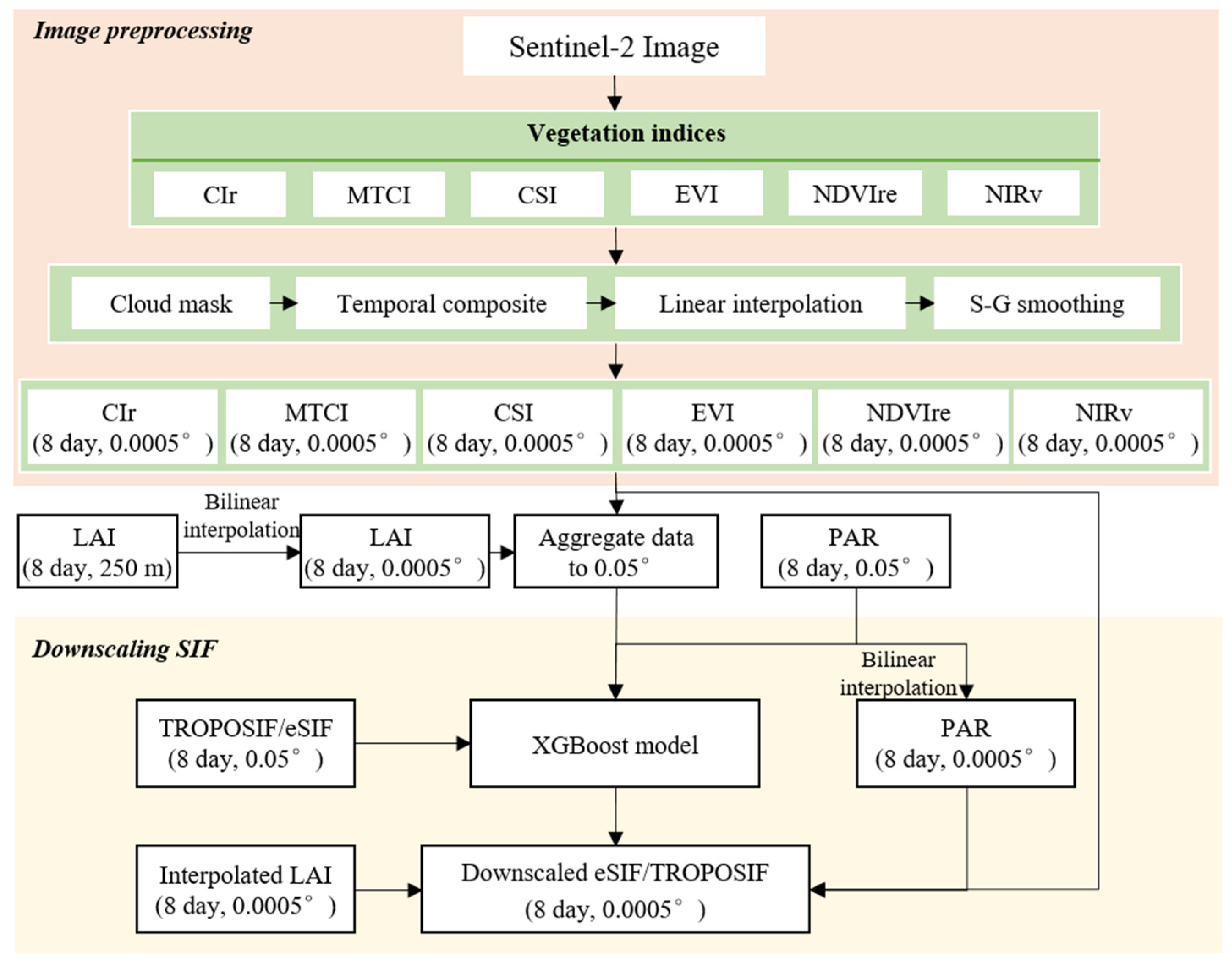
2.3.1. Downscaled SIF

(1)

Dataset construction

VIs and LAI have a strong correlation with SIF, and PAR plays a significant regulatory role in SIF. In this study, six VIs obtained from the Sentinel-2 satellite, along with LAI and PAR, were utilized as input parameters for the extreme gradient boosting (XGboost) model to downscale the TROPOSIF and eSIF data. Due to the low SIF values in the Saihanba area during the non-growing season, this study focused exclusively on data from the growing season (May–September). To match the resolution of the SIF data, the VIs for the 2020–2021 growing season were aggregated every 8 days to a resolution of 0.05°. Given the relatively small area of the Saihanba Forest Farm, the study area was appropriately expanded beyond Saihanba to ensure an adequate sample size for modeling, as shown in Figure 1.

(2)

Downscaling method based on XGBoost

The downscaling methods used by TROPOSIF and eSIF employ XGBoost. XGBoost is an advanced version of the gradient-boosted decision tree (GBDT) that constructs enhanced trees capable of handling complex nonlinear relationships [26,45]. Owing to its remarkable speed, accuracy, and efficiency, XGBoost has become widely adopted in the remote sensing community as a preferred machine learning algorithm. It has been employed in various downscaling applications, including in studies on crop yield [46], groundwater [47], and surface soil moisture [48]. In this study, the XGBoost algorithm implemented in the Python library was utilized for the analysis. The VIs, PAR, and LAI data at a resolution of 0.05° were used as input variables to model SIF. To evaluate the performance of the model, the data were divided into an 80% training set and a 20% test set. Given the influence of various parameters on the XGBoost model’s performance, the GridSearchCV method was adopted to optimize the parameters, with a specific emphasis on minimizing the root mean square error (RMSE). Through this process, the best-performing model was successfully identified and selected. The assumption was made that the modeling relationship between the 0.05° input variables and the SIF would not significantly differ at 0.0005°. Bilinear interpolation was used to resample the LAI from 250 m to 0.005° and the PAR data from 0.05° to 0.0005°. The final model incorporated VIs, PAR, and LAI data at a resolution of 0.0005° to downscale the SIF. Figure 2 illustrates the SIF downscaling process.

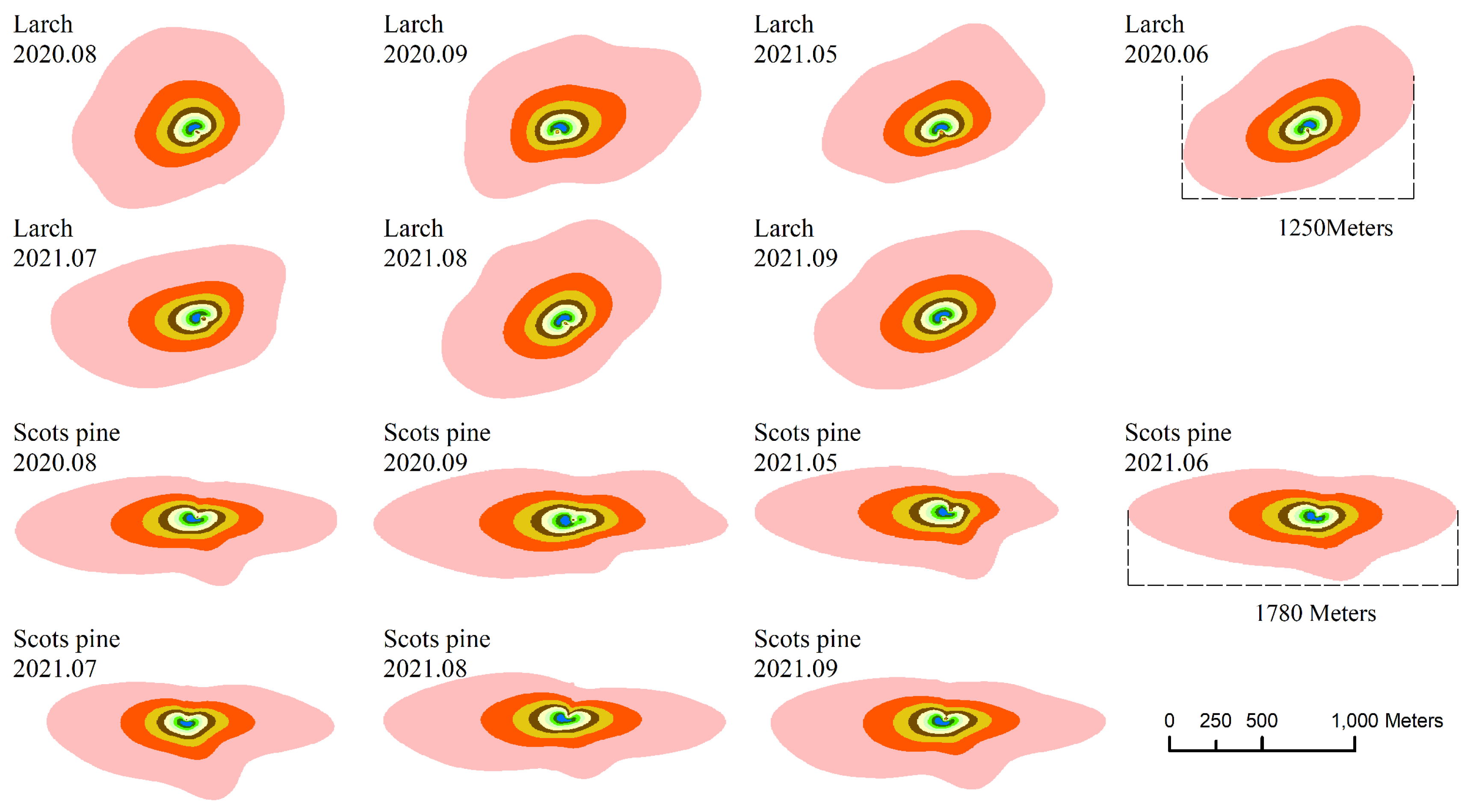
2.3.2. EC Flux Footprint Calculation

This study utilized the flux footprint prediction (FFP) model to estimate the footprint of the EC flux. The FFP model parameterizes the footprint in two dimensions, enabling a robust determination of the spatial extent and characteristics of the EC point footprint. For a more detailed understanding of the calculations used in footprint climatology, please refer to Kljun et al. [19]. Considering that vegetation’s carbon sequestration process primarily occurs during the daytime, footprint mapping was conducted at half-hour intervals throughout daylight hours. Subsequently, the data were aggregated over an 8-day period to generate spatial grids representing the contributions of the footprint. The contribution rate grid was classified by accumulating it around the flux tower in 10% increments, resulting in a classified map where the contribution rate was less than 90%. To facilitate the observation of the seasonal variation characteristics of the footprint contribution rate, monthly maps were also created for the growing season (Figure 3).

2.3.3. Validation of Downscaled SIF

The SIF from the SCOPE 2.1 model was compared with the downscaled SIF at the two flux sites to assess the effectiveness of the downscaled SIF. SCOPE is a one-dimensional model capable of simulating radiation transfer, energy balance, and photosynthesis, as well as SIF from individual leaves within the canopy and the total emitted SIF spectrum of chlorophyll fluorescence [49]. It is widely used for seasonal SIF estimation. The simulation range was set to 500 m around the flux towers, assuming homogeneity of the forest canopy and uniform atmospheric conditions within this range. The input parameters for the SCOPE model in this study are detailed in Appendix A. To match the timing of the downscaled SIF, the simulated half-hourly SIF was aggregated to 8 days.

2.3.4. Evaluation of the Relationship between GPP and Downscaled SIF

The coefficients of determination (R²) obtained from linear regression were employed to assess the degrees of linear association between GPP and three different SIF datasets: raw 0.05° SIF, downscaled SIF EC footprint-averaged (SIF_ECA), and downscaled SIF EC footprint-weighted (SIF_ECW). This analysis aimed to validate and assess the correlation between the downscaled SIF and GPP. SIF_ECA represents the average SIF value across 90% of the cumulative EC flux footprint range. On the other hand, SIF_ECW was calculated by assigning a weight to each flux footprint contribution within the 0–10%, 10–20%, ⋯, 70–80%, and 80–90% ranges. To ensure the sum of the weighting coefficients of SIF is 1, each part has a weight of 10/90 (as shown in Equation (1)).

$${\mathrm{SIF}}_{\mathrm{ECW}}={\displaystyle \sum _{\mathrm{k}=1}^{\mathrm{N}1}\frac{{\mathrm{SIF}}_{\mathrm{k}}}{\mathrm{N}1}}\times \frac{10}{90}+{\displaystyle \sum _{\mathrm{k}=1}^{\mathrm{N}2}\frac{{\mathrm{SIF}}_{\mathrm{k}}}{\mathrm{N}2}}\times \frac{10}{90}+\cdots {\displaystyle \sum _{\mathrm{k}=1}^{\mathrm{N}8}\frac{{\mathrm{SIF}}_{\mathrm{k}}}{\mathrm{N}8}}\times \frac{10}{90}+{\displaystyle \sum _{\mathrm{k}=1}^{\mathrm{N}9}\frac{{\mathrm{SIF}}_{\mathrm{k}}}{\mathrm{N}9}}\times \frac{10}{90}$$

(1)

The variables N1 to N9 refer to the total number of pixels within the image that fall within each of the nine cumulative footprint ranges, from the range of 0–10% to 80–90%. SIF_k represents the value of SIF for the specific pixel k located within the corresponding footprint range.

Additionally, the EC flux footprint-averaged VI (VI_ECA) and EC flux footprint-weighted VI (VI_ECW) were computed using an identical approach to assess variations in the correlation between VI_ECA and GPP, as well as between VI_ECW and GPP. It is worth noting that EC observations in the Saihanba area began on 1 August 2020, while the SIF and VIs data were from 2020 to 2021. Therefore, this study of the correlation between SIF, VIs, and GPP considered only data after 1 August 2020.

3. Results

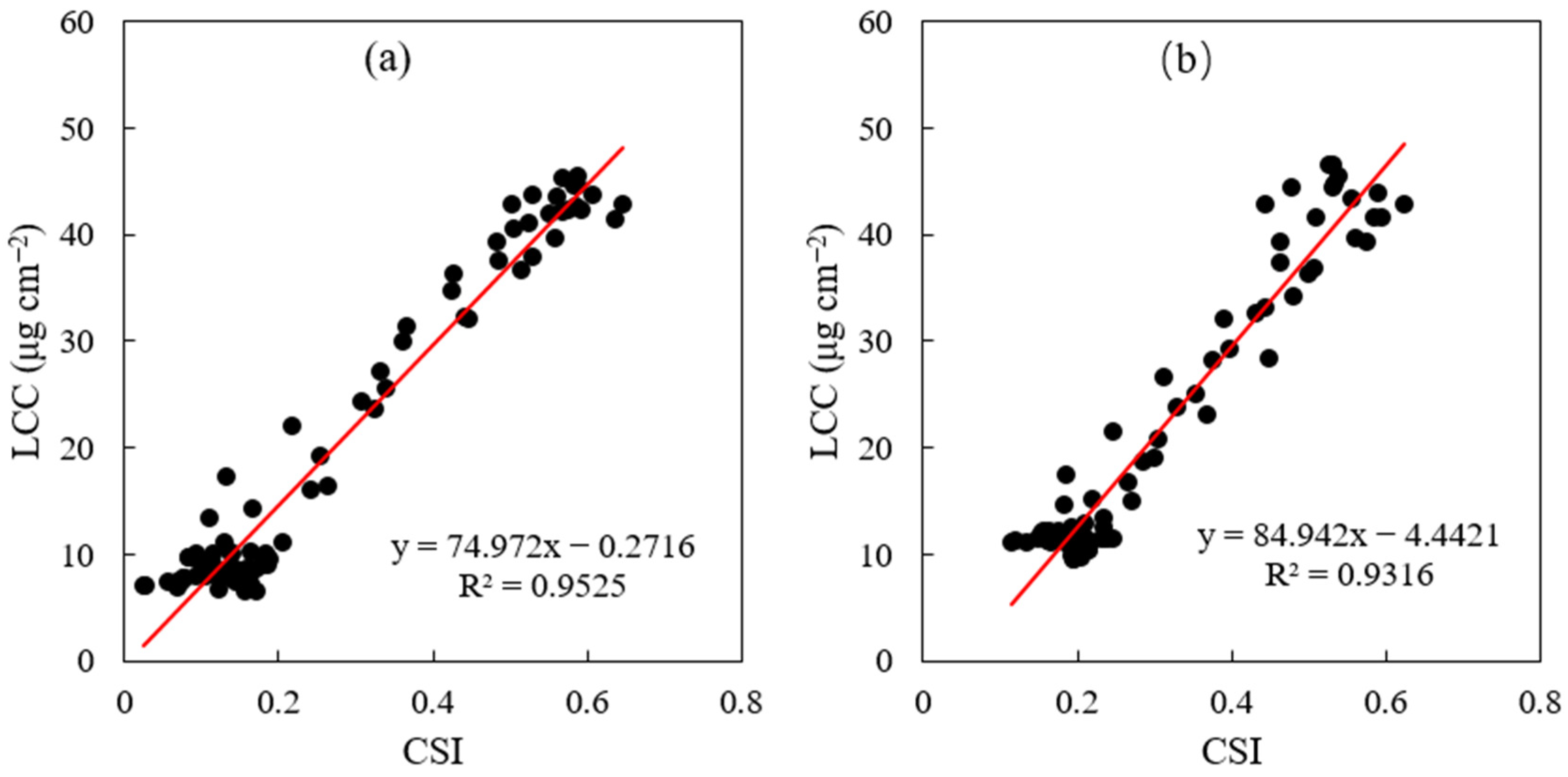
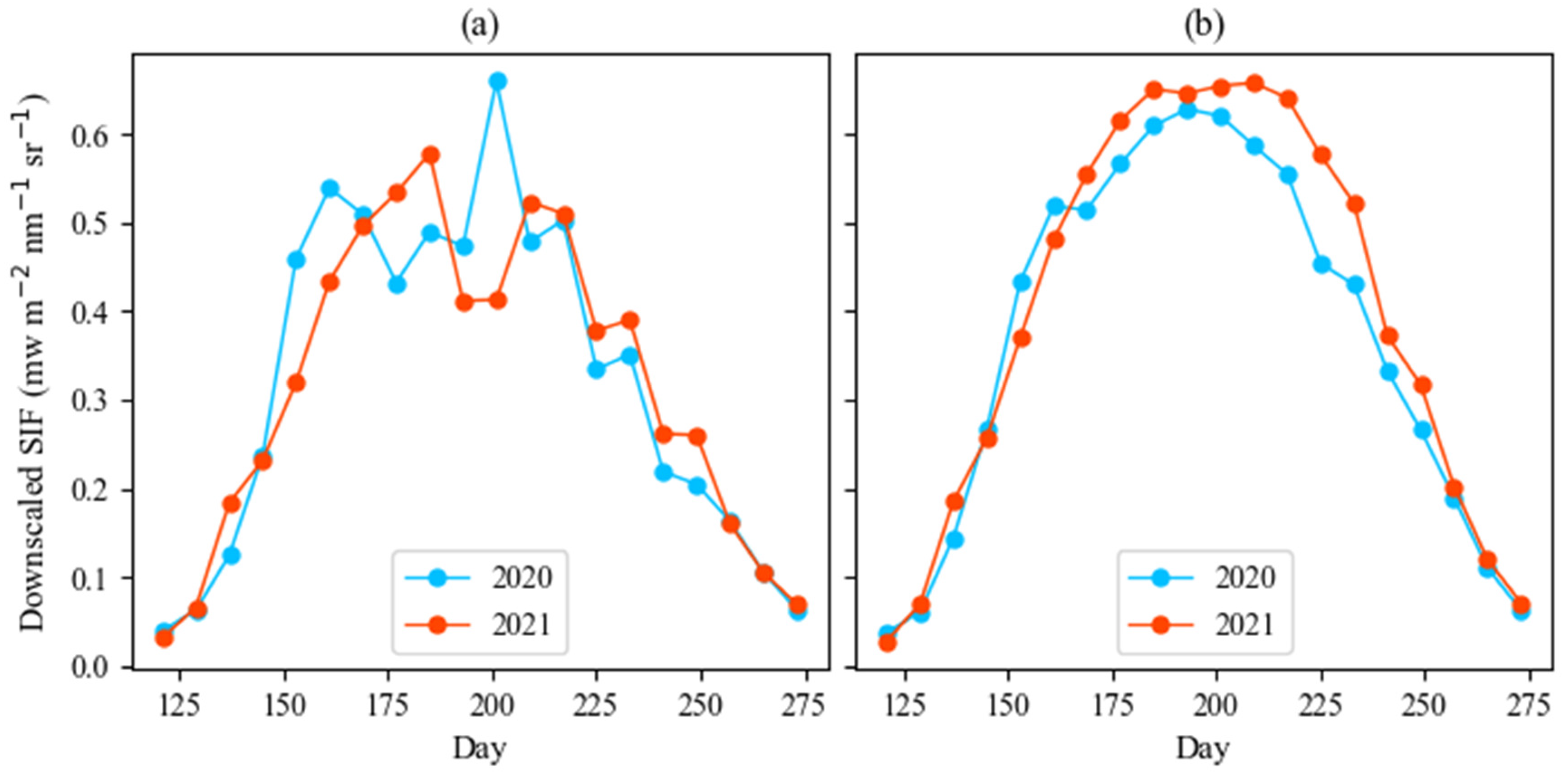
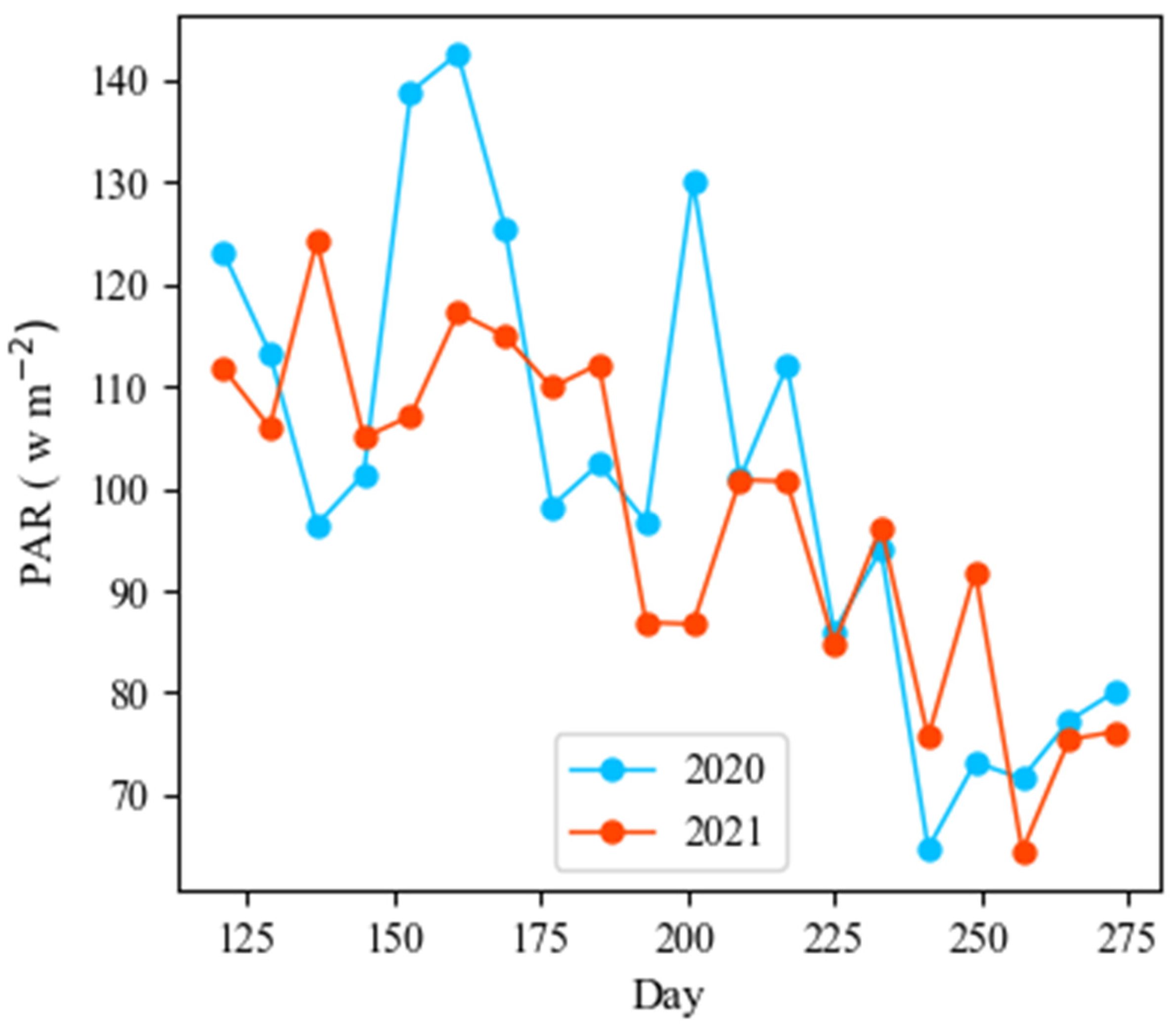
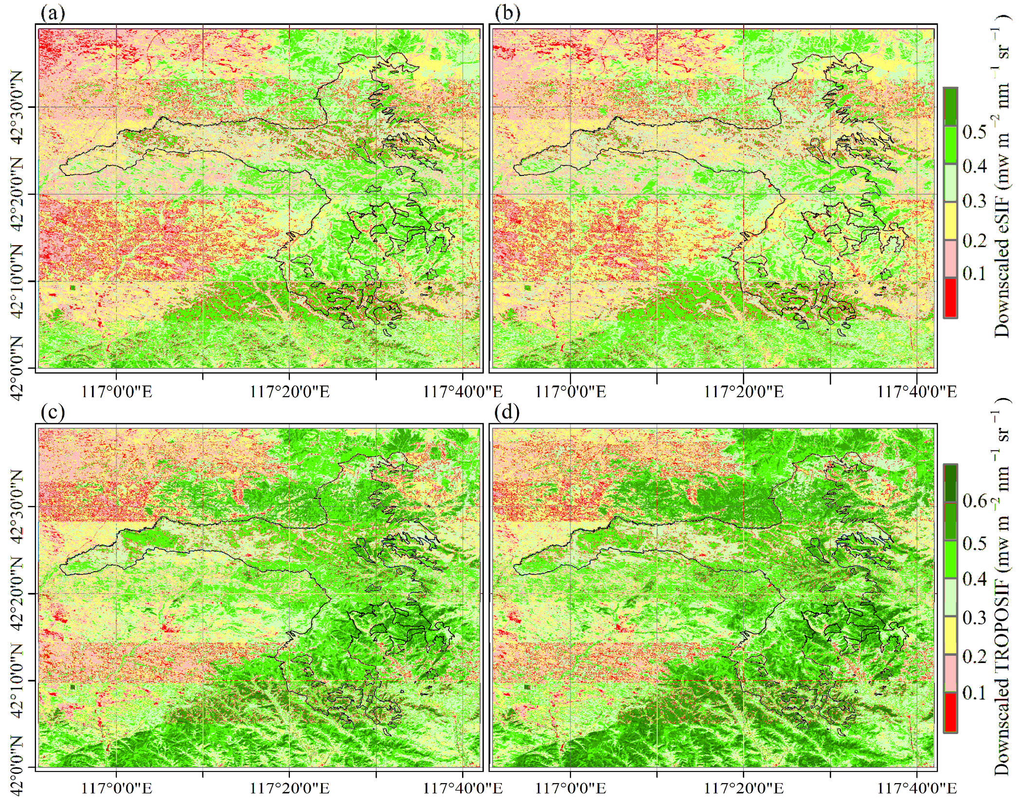
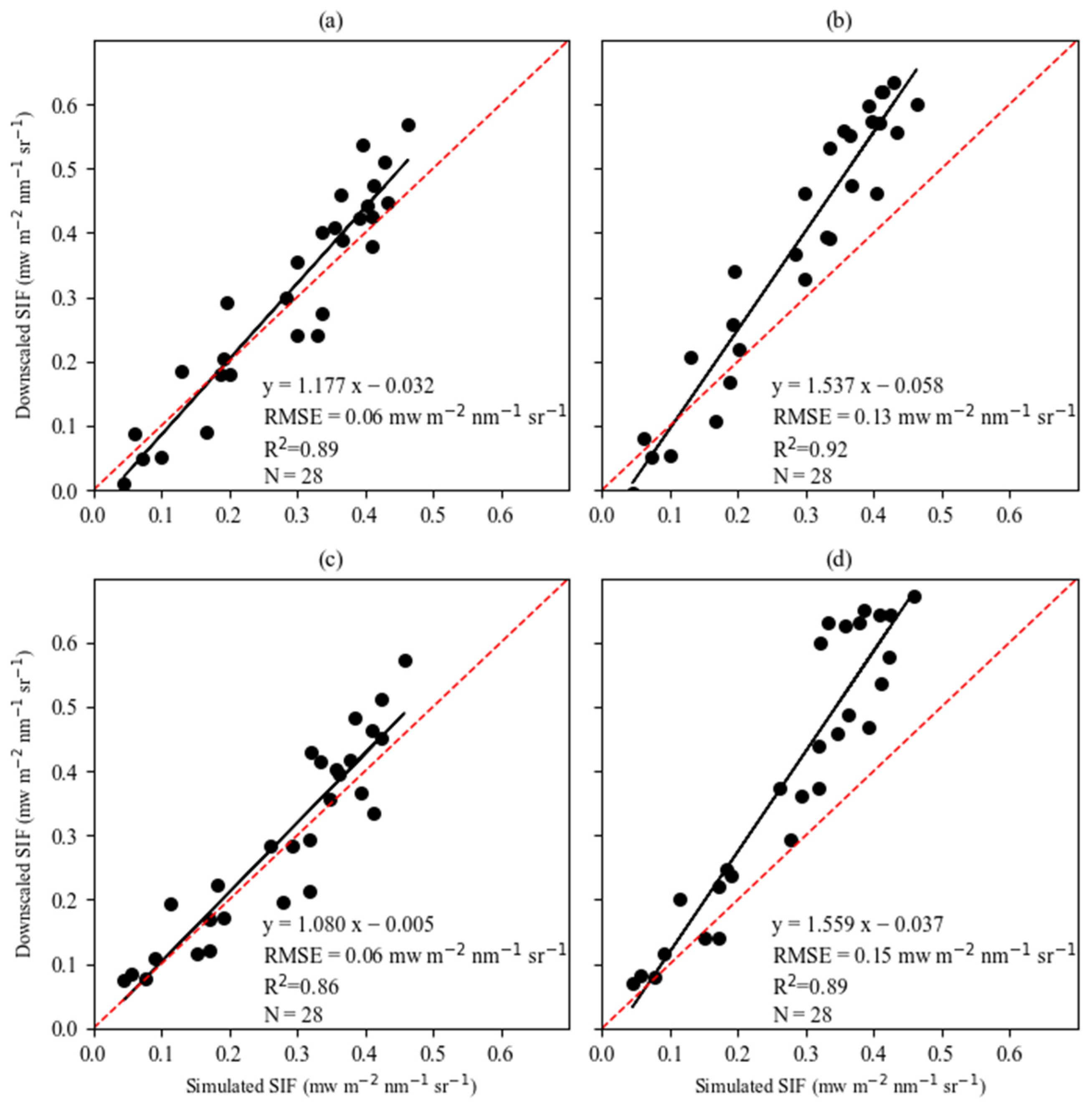
3.1. Downscaled SIF Performance

The spatial distributions of the 2020 and 2021 growing seasons’ downscaled SIF averages are shown in Figure 4. Notably, both the downscaled TROPOSIF and eSIF exhibited similar spatial patterns, but the values of TROPOSIF are slightly higher than those of eSIF. This is because TROPOSIF amplifies instantaneous SIF under clear-sky conditions to daily averages, while eSIF considers radiation amplification to daily averages under all weather changes, thus representing clear-sky TROPOSIF downscaled higher than eSIF considering all weather conditions. Additionally, the average downscaled eSIF values for the study area in 2020 and 2021 are both 0.32 mw m⁻² nm⁻¹ sr⁻¹ and are also spatially similar (Figure 4a,b). The mean downscaled TROPOSIF value in 2021 (0.40 mw m⁻² nm⁻¹ sr⁻¹) was greater than that in 2020 (0.37 mw m⁻² nm⁻¹ sr⁻¹), and in most regions spatially, the values in 2021 were greater than those in 2020. This is because TROPOSIF represents SIF under clear-sky conditions, while eSIF represents SIF under all weather conditions, and the seasonal patterns of SIF under different weather conditions differ (Figure A3). The PAR in the study area during the summer of 2021 was significantly lower than that of 2020 (Figure A4), indicating that there may have been more cloudy days in 2021. Therefore, the production of SIF data should consider all weather conditions, as they may not only cause biases in seasonal variations in SIF but also errors in interannual variations.

In the Saihanba region, a strong linear relationship was observed between the downscaled SIF and the SIF simulated by the SCOPE model at the two flux sites (Figure 5, R² ranging from 0.86 to 0.93). The relationship between the downscaled SIF and the simulated SIF at the SHB1 site was superior to that at the SHB2 site, and the relationship between the downscaled TROPOSIF and the simulated SIF at both sites was better than that with the eSIF. It is worth noting that the relationship between the downscaled eSIF and the simulated SIF tended to be closer to a 1:1 linear relationship. Additionally, the RMSE between the downscaled eSIF and the simulated SIF was 0.06 mw m⁻² nm⁻¹ sr⁻¹ at both sites, which is highly satisfactory. In conclusion, the strong relationship between the downscaled SIF and the modeled SIF indicates the high accuracy of the downscaled SIF results.

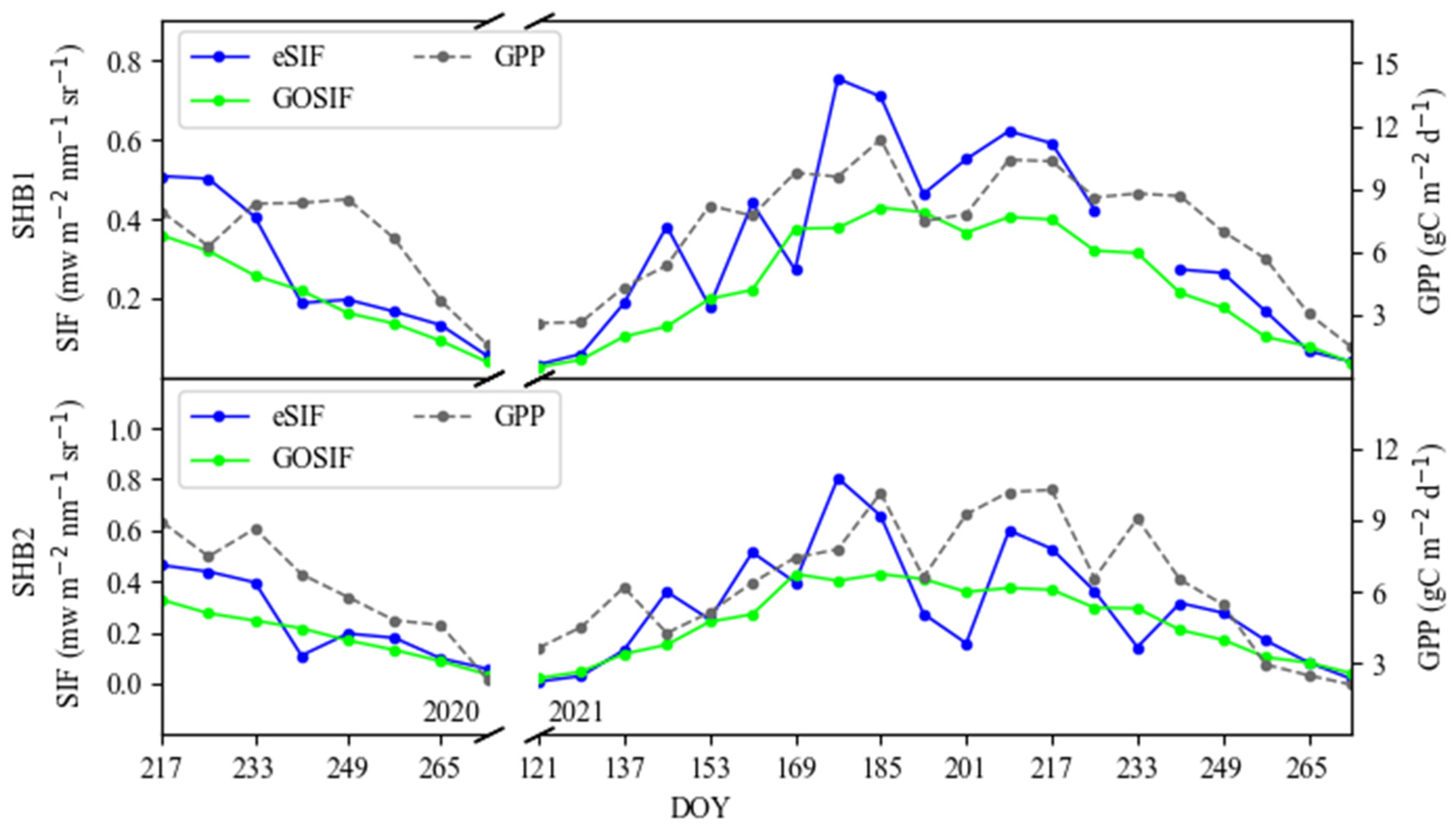
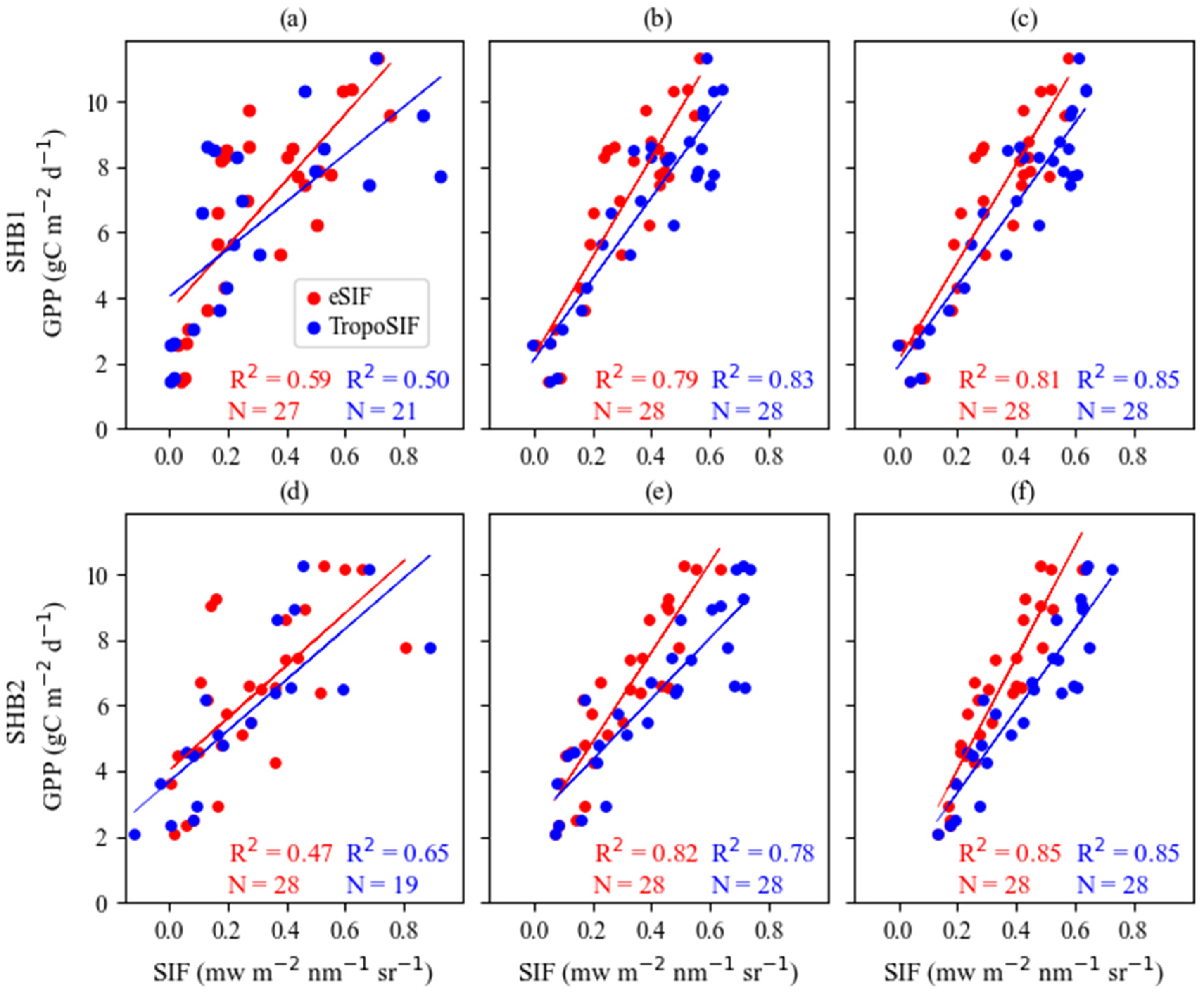
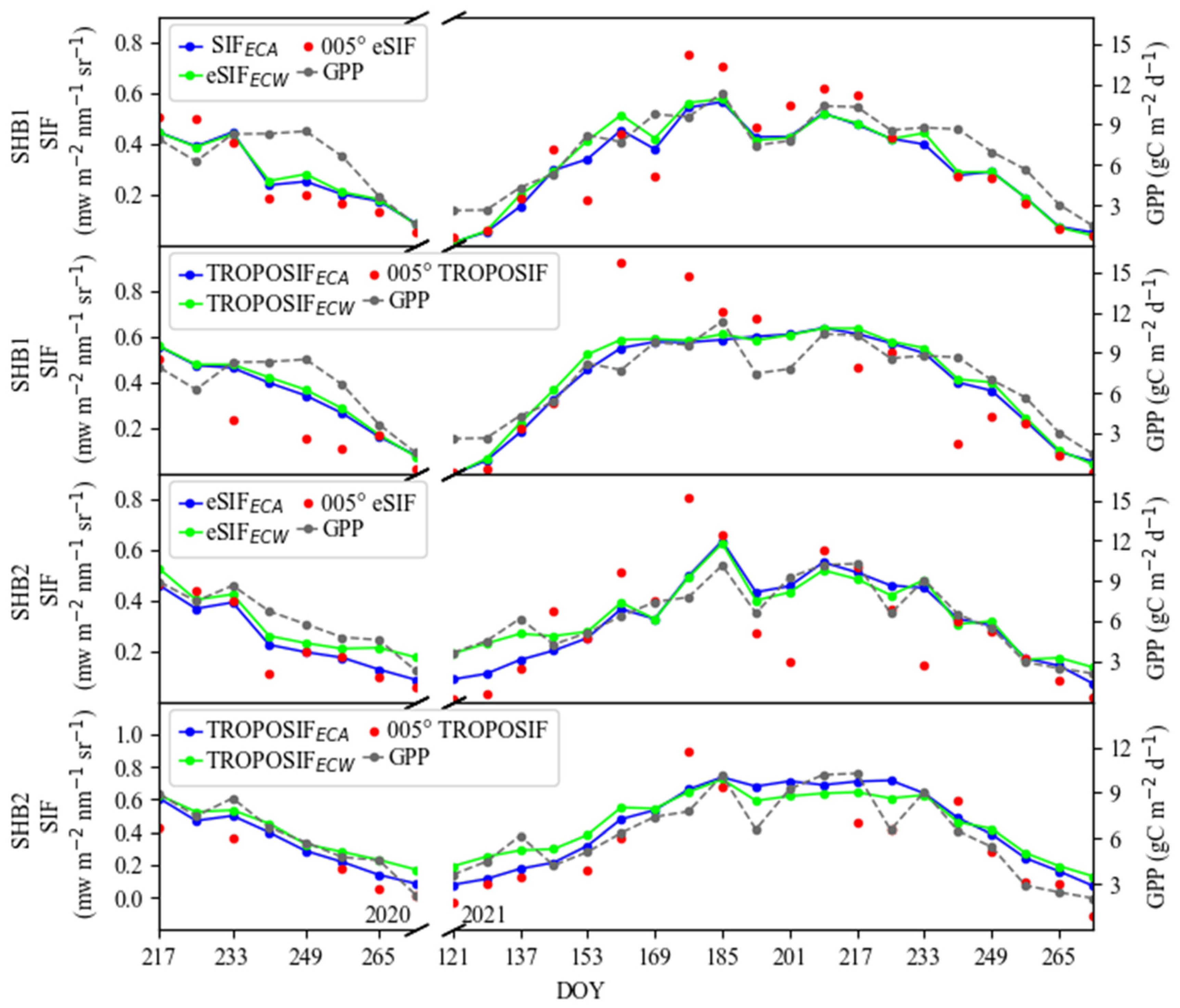
3.2. Comparison of Downscaled SIF and GPP

Figure 6 illustrates the correlation between three observational scales of SIF (0.05° SIF, SIF_ECA, SIF_ECW) and the GPP values at the two flux sites. Across both sites, the correlation order between the three observational scales of SIF and GPP was as follows: SIF_ECW > SIF_ECA > 0.05° SIF. The correlation between 0.05° SIF and GPP was relatively weak (R² ranging from 0.47 to 0.65), while the correlation between SIF_ECW and SIF_ECA with GPP was significantly enhanced (R² ranging from 0.78 to 0.85). Under the downscaling condition of SHB1, the correlation between TROPOSIF (SIF_ECW, SIF_ECA) and GPP surpassed that of eSIF, whereas at the SHB2 site, the relationship between eSIF’s SIF_ECA and GPP was superior to that with TROPOSIF, while SIF_ECW remained equivalent. These results indicate a substantial error between coarse-resolution SIF and GPP, while the relationship between the GPP matched to the flux footprints and the SIF was significantly improved. Different observational scales revealed significant differences in the linear fitting performance between SIF and GPP, emphasizing the crucial role of maintaining footprint consistency for accurately estimating their linear relationship.

Figure 7 illustrates the seasonal variations in the SIF (0.05° SIF, SIF_ECA, SIF_ECW) and GPP at the SHB1 and SHB2 sites. The seasonal variations in the 0.05° eSIF and TROPOSIF show considerable deviations from the GPP variation curves at both sites. Post-downscaling, eSIF (eSIF_ECA, eSIF_ECW) and TROPOSIF (TROPOSIF_ECA, TROPOSIF_ECW) exhibited better correspondence with the GPP variation curves. However, during periods of localized GPP decrease, the downscaled TROPOSIF failed to decrease accordingly, while eSIF followed the GPP variation, indicating a more consistent seasonal pattern in downscaled eSIF. For the flux footprint-weighted and -averaged SIF, the weighted SIF showed significant improvements in localized details compared to the averaged SIF.

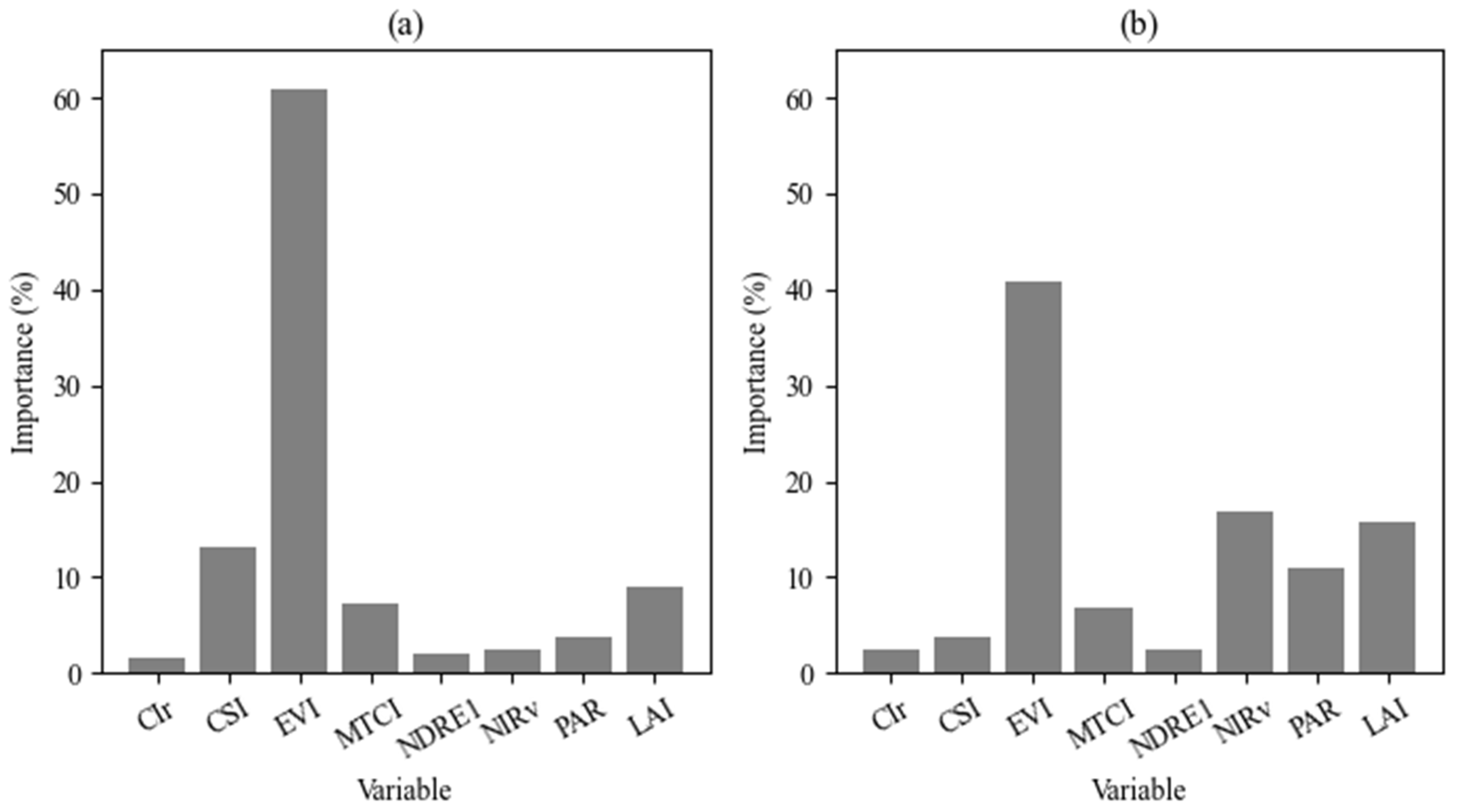
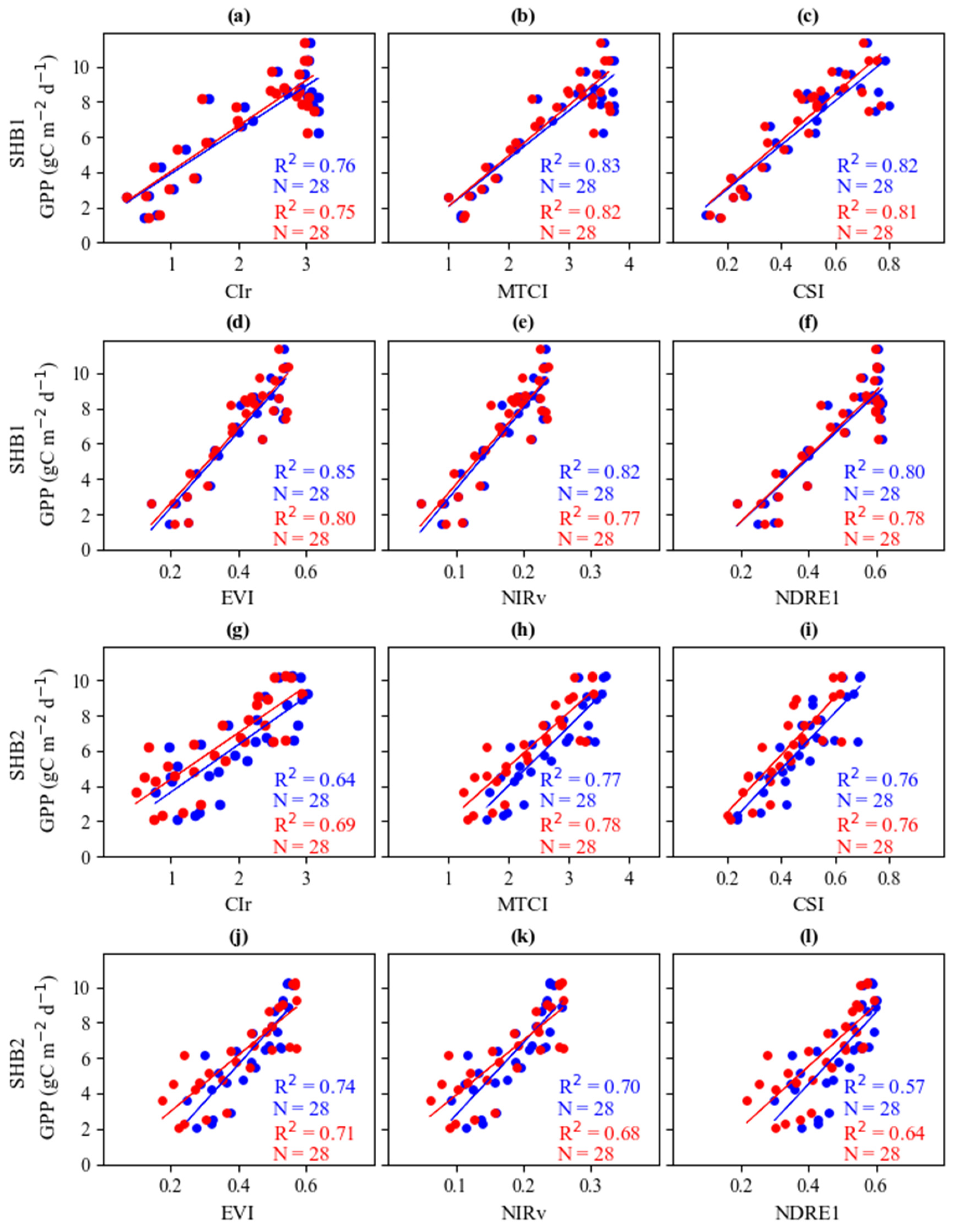
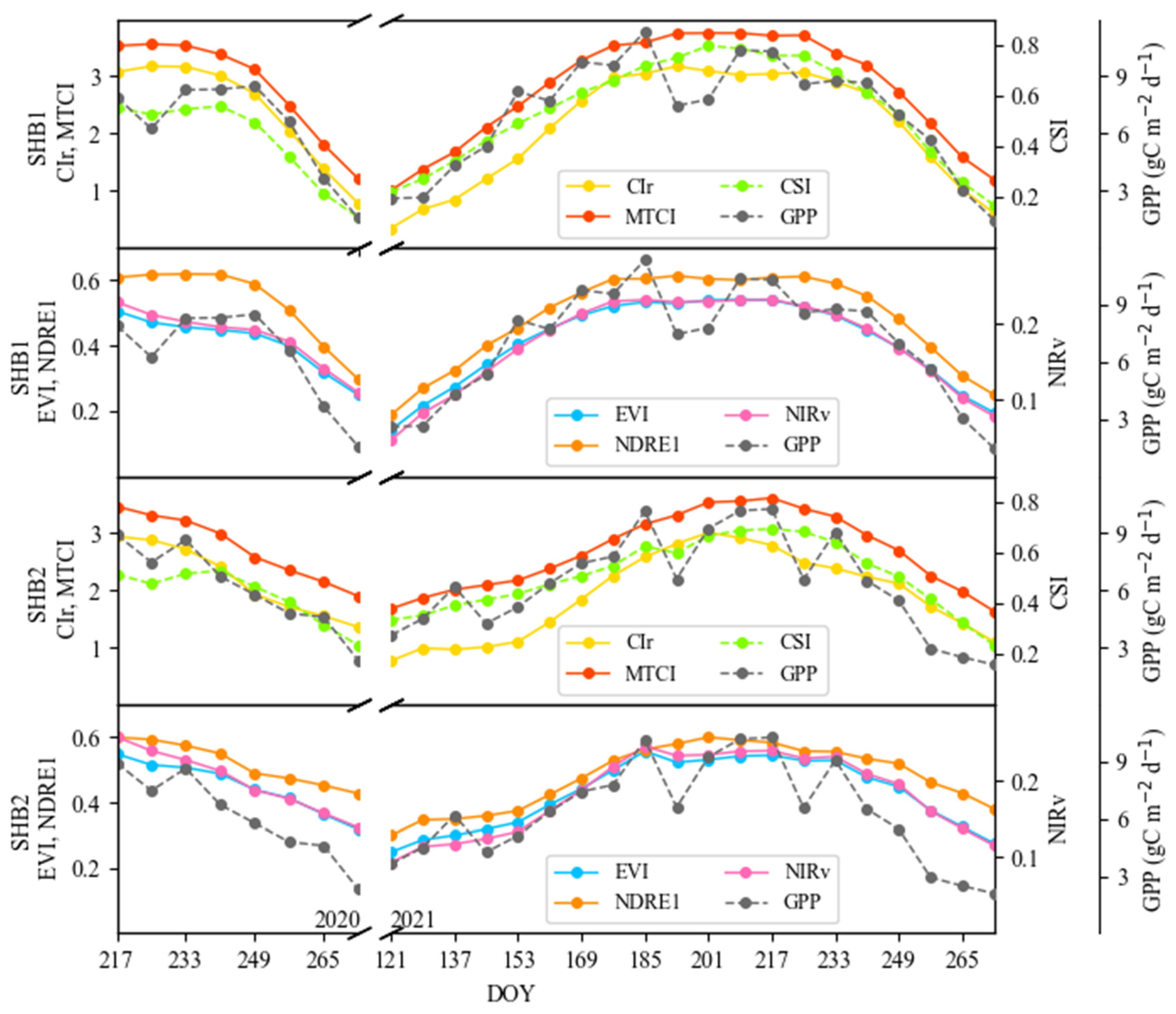
3.3. Comparison between VIs and GPP

At both the SHB1 and SHB2 sites, Figure 8 illustrates the linear relationships between the VI_ECA and GPP, as well as between the VI_ECW and GPP. There were significant differences in the VI-GPP relationships between the two sites. At the SHB1 site, all VI_ECA and VI_ECW exhibited strong linear relationships with the GPP (with the R² ranging between 0.75 and 0.85), and the relationship between the VI_ECW and GPP (with the R² ranging from 0.76 to 0.85) showed improvement compared to the VI_ECA and GPP (with the R² ranging from 0.75 to 0.82). Notably, the relationship between the EVI_ECW and GPP was the strongest, with an R² of 0.85. In contrast, at the SHB2 site, the linear relationships between the VIs (both VI_ECW and VI_ECA) and the GPP were generally weaker, with each VI performing worse than at the SHB1 site.

At the SHB1 site, the R² values between the VI_ECW and GPP for all VIs were superior to those between the VI_ECA and GPP. However, at the SHB2 site, only the R² values between the VI_ECW and GPP for NIRv and EVI were higher than those between the VI_ECA and GPP. Furthermore, at the SHB1 site, the fitted lines of the VI_ECW and GPP closely approximate those of the VI_ECA and GPP, whereas at the SHB2 site, there is a noticeable distance between the fitted lines of the VI_ECW and GPP compared to those of the VI_ECA and GPP. These results indicate that at the SHB1 site, the values of the VI_ECW were relatively close to those of the VI_ECA, while at the SHB2 site, there was a significant disparity between the values of the VI_ECW and the VI_ECA. This discrepancy is attributed to the more homogeneous underlying surface at the SHB1 site compared to the greater spatial heterogeneity at the SHB2 site. Additionally, these findings suggest that at flux sites with complex underlying landscapes, the relationship between the VIs and GPP is generally poor and unstable.

Figure 9 illustrates the seasonal variations in the VI_ECW and GPP. At the SHB1 site, throughout the entire growing season, the trends of the VI_ECW and GPP exhibit a relative correspondence. However, in localized areas, such as during the decline in the GPP in the summer, the VI_ECW failed to decrease correspondingly with the GPP. At the SHB2 site, the seasonal variations in the VI_ECW and GPP showed a significant difference. Particularly in the spring and autumn, the relationship between the VI_ECW and GPP was evidently mismatched. Furthermore, during the summer period of GPP decline, the VI_ECW at the SHB2 site also did not exhibit a corresponding decrease. In conclusion, it is difficult for VIs to track the seasonal variations in GPP.

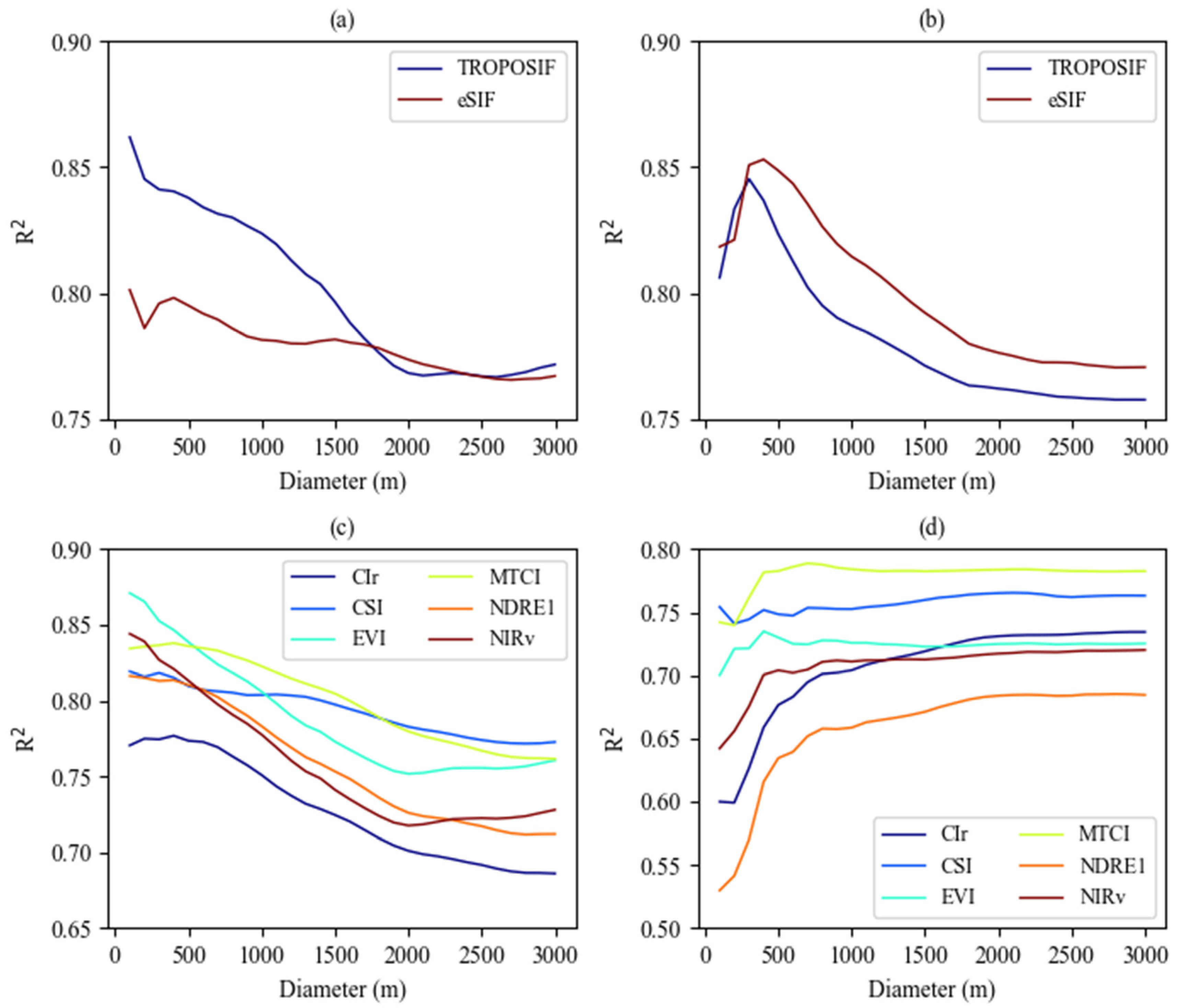
3.4. Relationships between SIF and GPP and between VIs and GPP across Different Observation Ranges

As the buffer zone diameter of flux sites varied, the relationship between the mean SIF (eSIF, TROPOSIF) and GPP, as well as the relationship between the mean VIs and GPP, changed, as depicted in Figure 10. At both sites, the R² values for eSIF and TROPOSIF with respect to GPP decreased as the buffer zone diameter increased, stabilizing at around 2000 m. At the SHB2 site, there was a process of increase followed by a decrease in the R² values for the SIF and TROPOSIF with respect to the GPP, with the inflection point occurring approximately at 500 m. The monthly-scale flux footprint diagrams (Figure 3) illustrate that at both forest sites, the footprint diameter within the area where the footprint contributed 80% was approximately 500 m, while within the region where the contribution reached 90%, the footprint diameter ranged from about 1000 m to 2000 m. This range closely aligns with the optimal range for the relationship between SIF and GPP. Therefore, to ensure the accuracy of the relationship between SIF and GPP, the observation range of SIF should ideally coincide with the flux footprint range as much as possible.

For VIs, at the SHB1 site, the pattern of R² values changing with the buffer zone diameter was similar to that for SIF and GPP: the R² decreased as the buffer zone diameter increased, stabilizing at around 2000 m. However, the distribution pattern at the SHB2 site was markedly different. For buffer zone diameters less than 500 m, the R² values for the VIs and GPP rapidly increased, stabilizing at around 500 m. This indicates that the VIs near the flux sites (<500 m) in SHB2 do not adequately represent the vegetation growth patterns in the flux source area, and in areas with significant landscape heterogeneity, the correlation between the VIs and GPP is poor. Furthermore, although the relationship between SIF and GPP weakened near the flux sites (<500 m) in SHB2, there was still a strong R² between SIF and GPP, indicating that SIF is more robustly associated with GPP compared to VIs.

4. Discussion

4.1. Comparison of TROPOSIF and eSIF Downscaling Data

The main advantage of eSIF over other reconstructed SIFs lies in its clearer and more straightforward relationship with the original SIF, making it more suitable for studying the “true” connection between SIF and GPP [27]. Using the GOSIF product as a representative of reconstructed SIF, the comparison of eSIF and reconstructed SIF in tracking the seasonal variations in GPP is shown in Figure A2. GOSIF exhibits smoother seasonal variation without corresponding changes with the decline in GPP, while eSIF demonstrates a more consistent variation pattern. This indicates that eSIF has a significant advantage in tracking seasonal changes in GPP. TROPOSIF is the true SIF directly retrieved from satellites. It is converted from instantaneous SIF on clear-sky days to daily-scale SIF by multiplying with a day-length scaling factor; hence, the daily-scale SIF can only represent SIF on clear-sky days [27,29]. In this study, the linear relationship between the downscaled TROPOSIF and the SCOPE-simulated SIF was slightly better than that with the eSIF (Figure 5), while the linear relationships of the eSIF and TROPOSIF with the GPP were comparable (Figure 6). The primary advantage of SIF lies in its ability to accurately reflect the vegetation’s photosynthetic capacity [2,50], making the development of SIF products capable of accurately tracking seasonal variations in GPP essential. However, compared to the eSIF, the downscaled TROPOSIF performed poorly in terms of consistency with seasonal variations in GPP. This is because the original TROPOSIF only represents SIF on clear days, thus affecting the downscaled results by not accounting for all weather conditions. As a result, the downscaled TROPOSIF failed to consider all weather conditions. The downscaled TROPOSIF values for the growing season of 2021 in the study area were significantly higher than those of 2020 (Figure A3), while the eSIF values remained almost equal between the two years (Figure 4), which could result in considerable errors in interannual variation. During the summer of 2021, the PAR data were notably lower compared to 2020 (Figure A4), suggesting the likelihood of more overcast days in 2021. Consequently, this could result in a considerable increase in the TROPOSIF value for 2021 compared to the SIF value across all weather conditions. Additionally, the downscaled model shows that the importance of PAR as an independent variable is low for TROPSOSIF (only 3.7%), while it is 10.9% for eSIF (Figure A5), indicating a weaker relationship between TROPSOSIF and PAR.

4.2. Impact of SIF-GPP Footprint Matching on Their Relationship

Matching the two downscaled SIF products to the EC flux footprints resulted in a noteworthy improvement in the relationship between SIF and GPP. This aspect, which has received limited attention in previous studies, has hindered comprehensive research on the SIF-GPP relationship. The linear correlation between the SIF_ECW and GPP shows improvement compared to the SIF_ECA, indicating a high correlation between the spatial patterns of SIF within the EC flux footprint and the contribution distribution of GPP. However, this pattern does not hold true for the VIs (Figure 8); even though the VIs showed similar patterns in SHB1, they disappeared in SHB2. The coupling of the SIF distribution in the flux footprint and the EC flux footprint supports the idea that SIF is a good proxy for GPP at a seasonal scale. The superior ability of SIF to spatially capture GPP may be attributed to its richer signal compared to the VIs. SIF is an inherent byproduct of photosynthesis, possessing both the physiological and structural characteristics of vegetation [21,22]. SIF can be decomposed into (NIRvP × Φ_F), where Φ_F represents the fluorescence emission efficiency of vegetation and physiological information, while NIRvP (NIRv × PAR) represents structural information [22]. Compared to NIRv, SIF incorporates two additional pieces of information: PAR and Φ_F. PAR reflects the source of photosynthetic energy, and its significance in relation to the SIF-GPP relationship is explained in Section 4.1. The physiological component Φ_F of SIF is its unique characteristic, making it the “essence” of SIF, as it is more directly associated with the photosynthetic process [22,27]. Due to the poor PAR information in downscaled TROPOSIF and VIs, the main differences between TROPOSIF and VIs are primarily reflected in Φ_F. However, at the SHB2 site, the linear relationship and seasonal patterns between downscaled TROPOSIF and GPP are notably superior to those of vegetation indices (Figure 6, Figure 7, Figure 8 and Figure 9), indicating the crucial importance of the spatial–temporal distribution of Φ_F in modulating the relationship between SIF and GPP. This can also be observed in Figure 10d, where the spatial coverage of VIs at the SHB2 site does not adjust its relationship with GPP, whereas the spatial coverage of TROPOSIF is closely related to GPP, further highlighting the essential role of Φ_F in regulating SIF. Furthermore, recent studies have verified the richer spatial information of SIF compared to that of the VIs. For example, Tagliabue et al. [51] estimated plant functional diversity using the NDVI, hyperspectral coefficient of variation (CV), and SIF, finding that SIF was more accurate than the NDVI and hyperspectral CV. Bandopadhyay et al. [52] discovered that SIF was closely related to the functional diversity of peatland vegetation and was more successful than VIs in capturing different vegetation signals from extremely heterogeneous peatland biomes.

4.3. Relationship between SIF and GPP at Different Scales

The spatial extent of SIF observations significantly influences its relationship with GPP at flux tower sites, such as SHB1 and SHB2. As the distance from the tower increases, the R² between the SIF and the GPP decreases notably. While it would be ideal to match the observed range of the SIF to the flux footprint of the GPP, the practical challenges of mapping the footprint of the GPP flux make this task complex and often infeasible. Figure 10 illustrates that restricting the observation range to specific areas can partially improve the relationship between SIF and GPP. At the SHB1 and SHB2 sites, a diameter of approximately 500 m still demonstrated a strong correlation between the SIF and GPP, corresponding precisely to the distance where the cumulative contribution of flux footprints from both sites reached 80%. Chu et al. [17] delineated the footprint range of 214 AmeriFlux sites, primarily defined as the maximum distance from the tower to the 80% contour of monthly footprint climatologies, ranging mainly between 100 m and 450 m. Hence, to mitigate errors arising from observational scales, it is crucial to refine the observational range using high-resolution SIF data. Furthermore, spatial heterogeneity also constrains the relationship between SIF and GPP. At the SHB1 site, as the distance from the tower increased, the linear relationship between the SIF and GPP consistently declined. However, at the SHB2 site, within 250 m of the observation tower, the relationship between the SIF and GPP actually increased with distance (Figure 10b). This is primarily due to the high spatial heterogeneity of the landscape at the SHB2 site (Figure 1). Research by Zhang et al. [53] found that spatial heterogeneity had a lesser impact on SIF measurements with larger measurement footprints, meaning that observations with larger footprints are more representative than those with smaller footprints. Therefore, in this study, when the observational footprint was appropriately expanded, the insufficient representativeness of SIF due to spatial heterogeneity might have been mitigated. In conclusion, emphasizing the representativeness of in situ SIF measurements is essential for elucidating the mechanisms between SIF and GPP and providing reliable observational data for satellite-based SIF validation [53].

5. Conclusions

In this study, coarse-resolution SIF data for the Saihanba region were downscaled to a higher resolution (0.0005°), and the effects of downscaling TROPOSIF data and eSIF data were compared. The results demonstrate that both the downscaled TROPOSIF and eSIF data exhibited a strong linear relationship with SIF simulated by the SCOPE model. Notably, the downscaled eSIF data showed a more consistent seasonal variation pattern with the GPP, indicating its greater suitability for studying the relationship between SIF and GPP. Furthermore, the comparison of the linear relationships of coarse-resolution SIF, SIF_ECA, and SIF_ECW with GPP revealed that the relationship between SIF_ECW and GPP was the strongest. This indicates that matching the SIF with the flux footprint can improve the relationship between the SIF and the GPP. Additionally, an examination of the relationship between the SIF and GPP at varying distances from the flux tower revealed that this relationship deteriorated as the distance increased, reaching its weakest point beyond 1 km from the flux tower. Moreover, at the SHB2 site, which is characterized by significant landscape heterogeneity, the relationship between the VIs and GPP was found to be poor, with no clear pattern in the relationship between the observation scale and GPP. Overall, these findings emphasize the importance of using high-resolution SIF data and ensuring consistency between the flux footprint and SIF observations for accurately assessing the relationship between the SIF and the GPP.

References

1. Gu, L.; Han, J.; Wood, J.D.; Chang, C.Y.Y.; Sun, Y. Sun-induced Chl fluorescence and its importance for biophysical modeling of photosynthesis based on light reactions. New Phytol. 2019, 223, 1179–1191. [Google Scholar] [CrossRef] [PubMed]
2. Magney, T.S.; Bowling, D.R.; Logan, B.A.; Grossmann, K.; Stutz, J.; Blanken, P.D.; Burns, S.P.; Cheng, R.; Garcia, M.A.; Köhler, P. Mechanistic evidence for tracking the seasonality of photosynthesis with solar-induced fluorescence. Proc. Natl. Acad. Sci. USA 2019, 116, 11640–11645. [Google Scholar] [CrossRef] [PubMed]
3. Liu, Z.; Zhao, F.; Liu, X.; Yu, Q.; Wang, Y.; Peng, X.; Cai, H.; Lu, X. Direct estimation of photosynthetic CO2 assimilation from solar-induced chlorophyll fluorescence (SIF). Remote Sens. Environ. 2022, 271, 112893. [Google Scholar] [CrossRef]
4. Porcar-Castell, A.; Tyystjärvi, E.; Atherton, J.; Van der Tol, C.; Flexas, J.; Pfündel, E.E.; Moreno, J.; Frankenberg, C.; Berry, J.A. Linking chlorophyll a fluorescence to photosynthesis for remote sensing applications: Mechanisms and challenges. J. Exp. Bot. 2014, 65, 4065–4095. [Google Scholar] [CrossRef]
5. Li, X.; Xiao, J.; He, B.; Altaf Arain, M.; Beringer, J.; Desai, A.R.; Emmel, C.; Hollinger, D.Y.; Krasnova, A.; Mammarella, I. Solar-induced chlorophyll fluorescence is strongly correlated with terrestrial photosynthesis for a wide variety of biomes: First global analysis based on OCO-2 and flux tower observations. Glob. Chang. Biol. 2018, 24, 3990–4008. [Google Scholar] [CrossRef] [PubMed]
6. Sun, Y.; Frankenberg, C.; Wood, J.D.; Schimel, D.S.; Jung, M.; Guanter, L.; Drewry, D.T.; Verma, M.; Porcar-Castell, A.; Griffis, T.J. OCO-2 advances photosynthesis observation from space via solar-induced chlorophyll fluorescence. Science 2017, 358, eaam5747. [Google Scholar] [CrossRef]
7. Li, X.; Xiao, J. Mapping photosynthesis solely from solar-induced chlorophyll fluorescence: A global, fine-resolution dataset of gross primary production derived from OCO-2. Remote Sens. 2019, 11, 2563. [Google Scholar] [CrossRef]
8. Zhang, Z.; Zhang, Y.; Porcar-Castell, A.; Joiner, J.; Guanter, L.; Yang, X.; Migliavacca, M.; Ju, W.; Sun, Z.; Chen, S. Reduction of structural impacts and distinction of photosynthetic pathways in a global estimation of GPP from space-borne solar-induced chlorophyll fluorescence. Remote Sens. Environ. 2020, 240, 111722. [Google Scholar] [CrossRef]
9. Guanter, L.; Zhang, Y.; Jung, M.; Joiner, J.; Voigt, M.; Berry, J.A.; Frankenberg, C.; Huete, A.R.; Zarco-Tejada, P.; Lee, J.-E. Global and time-resolved monitoring of crop photosynthesis with chlorophyll fluorescence. Proc. Natl. Acad. Sci. USA 2014, 111, E1327–E1333. [Google Scholar] [CrossRef]
10. Kim, J.; Ryu, Y.; Dechant, B.; Lee, H.; Kim, H.S.; Kornfeld, A.; Berry, J.A. Solar-induced chlorophyll fluorescence is non-linearly related to canopy photosynthesis in a temperate evergreen needleleaf forest during the fall transition. Remote Sens. Environ. 2021, 258, 112362. [Google Scholar] [CrossRef]
11. Liu, Y.; Chen, J.M.; He, L.; Zhang, Z.; Wang, R.; Rogers, C.; Fan, W.; de Oliveira, G.; Xie, X. Non-linearity between gross primary productivity and far-red solar-induced chlorophyll fluorescence emitted from canopies of major biomes. Remote Sens. Environ. 2022, 271, 112896. [Google Scholar] [CrossRef]
12. Bai, J.; Zhang, H.; Sun, R.; Li, X.; Xiao, J.; Wang, Y. Estimation of global GPP from GOME-2 and OCO-2 SIF by considering the dynamic variations of GPP-SIF relationship. Agric. For. Meteorol. 2022, 326, 109180. [Google Scholar] [CrossRef]
13. Martini, D.; Sakowska, K.; Wohlfahrt, G.; Pacheco-Labrador, J.; van der Tol, C.; Porcar-Castell, A.; Magney, T.S.; Carrara, A.; Colombo, R.; El-Madany, T.S. Heatwave breaks down the linearity between sun-induced fluorescence and gross primary production. New Phytol. 2022, 233, 2415–2428. [Google Scholar] [CrossRef]
14. Xu, S.; Atherton, J.; Riikonen, A.; Zhang, C.; Oivukkamäki, J.; MacArthur, A.; Honkavaara, E.; Hakala, T.; Koivumäki, N.; Liu, Z. Structural and photosynthetic dynamics mediate the response of SIF to water stress in a potato crop. Remote Sens. Environ. 2021, 263, 112555. [Google Scholar] [CrossRef]
15. Wu, L.; Zhang, X.; Rossini, M.; Wu, Y.; Zhang, Z.; Zhang, Y. Physiological dynamics dominate the response of canopy far-red solar-induced fluorescence to herbicide treatment. Agric. For. Meteorol. 2022, 323, 109063. [Google Scholar] [CrossRef]
16. Huang, X.; Lin, S.; Li, X.; Ma, M.; Wu, C.; Yuan, W. How Well Can Matching High Spatial Resolution Landsat Data with Flux Tower Footprints Improve Estimates of Vegetation Gross Primary Production. Remote Sens. 2022, 14, 6062. [Google Scholar] [CrossRef]
17. Chu, H.; Luo, X.; Ouyang, Z.; Chan, W.S.; Dengel, S.; Biraud, S.C.; Torn, M.S.; Metzger, S.; Kumar, J.; Arain, M.A. Representativeness of Eddy-Covariance flux footprints for areas surrounding AmeriFlux sites. Agric. For. Meteorol. 2021, 301, 108350. [Google Scholar] [CrossRef]
18. Kong, J.; Ryu, Y.; Liu, J.; Dechant, B.; Rey-Sanchez, C.; Shortt, R.; Szutu, D.; Verfaillie, J.; Houborg, R.; Baldocchi, D.D. Matching high resolution satellite data and flux tower footprints improves their agreement in photosynthesis estimates. Agric. For. Meteorol. 2022, 316, 108878. [Google Scholar] [CrossRef]
19. Kljun, N.; Calanca, P.; Rotach, M.W.; Schmid, H.P. A simple two-dimensional parameterisation for Flux Footprint Prediction (FFP). Geosci. Model Dev. 2015, 8, 3695–3713. [Google Scholar] [CrossRef]
20. Zhou, H.; Liang, S.; He, T.; Wang, J.; Bo, Y.; Wang, D. Evaluating the spatial representativeness of the MODerate resolution image spectroradiometer albedo product (MCD43) at ameriflux sites. Remote Sens. 2019, 11, 547. [Google Scholar] [CrossRef]
21. Wang, N.; Yang, P.; Clevers, J.G.P.W.; Wieneke, S.; Kooistra, L. Decoupling physiological and non-physiological responses of sugar beet to water stress from sun-induced chlorophyll fluorescence. Remote Sens. Environ. 2023, 286, 113445. [Google Scholar] [CrossRef]
22. Dechant, B.; Ryu, Y.; Badgley, G.; Köhler, P.; Rascher, U.; Migliavacca, M.; Zhang, Y.; Tagliabue, G.; Guan, K.; Rossini, M. NIRVP: A robust structural proxy for sun-induced chlorophyll fluorescence and photosynthesis across scales. Remote Sens. Environ. 2022, 268, 112763. [Google Scholar] [CrossRef]
23. Zhang, Y.; Joiner, J.; Alemohammad, S.H.; Zhou, S.; Gentine, P. A global spatially contiguous solar-induced fluorescence (CSIF) dataset using neural networks. Biogeosciences 2018, 15, 5779–5800. [Google Scholar] [CrossRef]
24. Li, X.; Xiao, J. A global, 0.05-degree product of solar-induced chlorophyll fluorescence derived from OCO-2, MODIS, and reanalysis data. Remote Sens. 2019, 11, 517. [Google Scholar] [CrossRef]
25. Gensheimer, J.; Turner, A.J.; Köhler, P.; Frankenberg, C.; Chen, J. A convolutional neural network for spatial downscaling of satellite-based solar-induced chlorophyll fluorescence (SIFnet). Biogeosciences 2022, 19, 1777–1793. [Google Scholar] [CrossRef]
26. Chen, X.; Huang, Y.; Nie, C.; Zhang, S.; Wang, G.; Chen, S.; Chen, Z. A long-term reconstructed TROPOMI solar-induced fluorescence dataset using machine learning algorithms. Sci. Data 2022, 9, 427. [Google Scholar] [CrossRef] [PubMed]
27. Liu, X.; Liu, L.; Bacour, C.; Guanter, L.; Chen, J.; Ma, Y.; Chen, R.; Du, S. A simple approach to enhance the TROPOMI solar-induced chlorophyll fluorescence product by combining with canopy reflected radiation at near-infrared band. Remote Sens. Environ. 2023, 284, 113341. [Google Scholar] [CrossRef]
28. Köhler, P.; Frankenberg, C.; Magney, T.S.; Guanter, L.; Joiner, J.; Landgraf, J. Global retrievals of solar-induced chlorophyll fluorescence with TROPOMI: First results and intersensor comparison to OCO-2. Geophys. Res. Lett. 2018, 45, 10–456. [Google Scholar] [CrossRef] [PubMed]
29. Guanter, L.; Bacour, C.; Schneider, A.; Aben, I.; van Kempen, T.A.; Maignan, F.; Retscher, C.; Köhler, P.; Frankenberg, C.; Joiner, J. The TROPOSIF global sun-induced fluorescence dataset from the Sentinel-5P TROPOMI mission. Earth Syst. Sci. Data 2021, 13, 5423–5440. [Google Scholar] [CrossRef]
30. Zhang, J.; Xiao, J.; Tong, X.; Zhang, J.; Meng, P.; Li, J.; Liu, P.; Yu, P. NIRv and SIF better estimate phenology than NDVI and EVI: Effects of spring and autumn phenology on ecosystem production of planted forests. Agric. For. Meteorol. 2022, 315, 108819. [Google Scholar] [CrossRef]
31. Zhao, J.; Zhang, M.; Xiao, W.; Wang, W.; Zhang, Z.; Yu, Z.; Xiao, Q.; Cao, Z.; Xu, J.; Zhang, X. An evaluation of the flux-gradient and the eddy covariance method to measure CH4, CO2, and H2O fluxes from small ponds. Agric. For. Meteorol. 2019, 275, 255–264. [Google Scholar] [CrossRef]
32. Wutzler, T.; Lucas-Moffat, A.; Migliavacca, M.; Knauer, J.; Sickel, K.; Šigut, L.; Menzer, O.; Reichstein, M. Basic and extensible post-processing of eddy covariance flux data with REddyProc. Biogeosciences 2018, 15, 5015–5030. [Google Scholar] [CrossRef]
33. Lasslop, G.; Reichstein, M.; Papale, D.; Richardson, A.D.; Arneth, A.; Barr, A.; Stoy, P.; Wohlfahrt, G. Separation of net ecosystem exchange into assimilation and respiration using a light response curve approach: Critical issues and global evaluation. Glob. Chang. Biol. 2010, 16, 187–208. [Google Scholar] [CrossRef]
34. Zupanc, A. Improving Cloud Detection with Machine Learning. Available online: https://medium.com/sentinel-hub/improving-cloud-detection-with-machine-learning-c09dc5d7cf13 (accessed on 22 June 2024).
35. D’Andrimont, R.; Lemoine, G.; Van der Velde, M. Targeted grassland monitoring at parcel level using sentinels, street-level images and field observations. Remote Sens. 2018, 10, 1300. [Google Scholar] [CrossRef]
36. You, N.; Dong, J.; Huang, J.; Du, G.; Zhang, G.; He, Y.; Yang, T.; Di, Y.; Xiao, X. The 10-m crop type maps in Northeast China during 2017–2019. Sci. Data 2021, 8, 41. [Google Scholar] [CrossRef]
37. Gitelson, A.A.; Verma, S.B.; Vina, A.; Rundquist, D.C.; Keydan, G.; Leavitt, B.; Arkebauer, T.J.; Burba, G.G.; Suyker, A.E. Novel technique for remote estimation of CO2 flux in maize. Geophys. Res. Lett. 2003, 30. [Google Scholar] [CrossRef]
38. Dash, J.; Curran, P.J. The MERIS terrestrial chlorophyll index. Int. J. Remote Sens. 2004, 25, 5403–5413. [Google Scholar] [CrossRef]
39. Zhang, H.; Li, J.; Liu, Q.; Lin, S.; Huete, A.; Liu, L.; Croft, H.; Clevers, J.G.P.W.; Zeng, Y.; Wang, X. A novel red-edge spectral index for retrieving the leaf chlorophyll content. Methods Ecol. Evol. 2022, 13, 2771–2787. [Google Scholar] [CrossRef]
40. Huete, A.; Didan, K.; Miura, T.; Rodriguez, E.P.; Gao, X.; Ferreira, L.G. Overview of the radiometric and biophysical performance of the MODIS vegetation indices. Remote Sens. Environ. 2002, 83, 195–213. [Google Scholar] [CrossRef]
41. Sims, D.A.; Gamon, J.A. Relationships between leaf pigment content and spectral reflectance across a wide range of species, leaf structures and developmental stages. Remote Sens. Environ. 2002, 81, 337–354. [Google Scholar] [CrossRef]
42. Badgley, G.; Field, C.B.; Berry, J.A. Canopy near-infrared reflectance and terrestrial photosynthesis. Sci. Adv. 2017, 3, e1602244. [Google Scholar] [CrossRef]
43. Ma, H.; Liang, S. Development of the GLASS 250-m leaf area index product (version 6) from MODIS data using the bidirectional LSTM deep learning model. Remote Sens. Environ. 2022, 273, 112985. [Google Scholar] [CrossRef]
44. Ryu, Y.; Jiang, C.; Kobayashi, H.; Detto, M. MODIS-derived global land products of shortwave radiation and diffuse and total photosynthetically active radiation at 5 km resolution from 2000. Remote Sens. Environ. 2018, 204, 812–825. [Google Scholar] [CrossRef]
45. Chen, T.; Guestrin, C. Xgboost: A Scalable Tree Boosting System. In Proceedings of the 22nd ACM SIGKDD International Conference on Knowledge Discovery and Data Mining, San Francisco, CA, USA, 13–17 August 2016; Association for Computing Machinery: New York, NY, USA, 2016; pp. 785–794. [Google Scholar]
46. Folberth, C.; Baklanov, A.; Balkovič, J.; Skalský, R.; Khabarov, N.; Obersteiner, M. Spatio-temporal downscaling of gridded crop model yield estimates based on machine learning. Agric. For. Meteorol. 2019, 264, 1–15. [Google Scholar] [CrossRef]
47. Zhang, J.; Liu, K.; Wang, M. Downscaling groundwater storage data in China to a 1-km resolution using machine learning methods. Remote Sens. 2021, 13, 523. [Google Scholar] [CrossRef]
48. Liu, Y.; Xia, X.; Yao, L.; Jing, W.; Zhou, C.; Huang, W.; Li, Y.; Yang, J. Downscaling satellite retrieved soil moisture using regression tree-based machine learning algorithms over Southwest France. Earth Space Sci. 2020, 7, e2020EA001267. [Google Scholar] [CrossRef]
49. Yang, P.; Prikaziuk, E.; Verhoef, W.; van Der Tol, C. SCOPE 2.0: A model to simulate vegetated land surface fluxes and satellite signals. Geosci. Model Dev. 2020, 2020, 4697–4712. [Google Scholar] [CrossRef]
50. Mohammed, G.H.; Colombo, R.; Middleton, E.M.; Rascher, U.; van der Tol, C.; Nedbal, L.; Goulas, Y.; Pérez-Priego, O.; Damm, A.; Meroni, M. Remote sensing of solar-induced chlorophyll fluorescence (SIF) in vegetation: 50 years of progress. Remote Sens. Environ. 2019, 231, 111177. [Google Scholar] [CrossRef] [PubMed]
51. Tagliabue, G.; Panigada, C.; Celesti, M.; Cogliati, S.; Colombo, R.; Migliavacca, M.; Rascher, U.; Rocchini, D.; Schüttemeyer, D.; Rossini, M. Sun–induced fluorescence heterogeneity as a measure of functional diversity. Remote Sens. Environ. 2020, 247, 111934. [Google Scholar] [CrossRef]
52. Bandopadhyay, S.; Rastogi, A.; Rascher, U.; Rademske, P.; Schickling, A.; Cogliati, S.; Julitta, T.; Mac Arthur, A.; Hueni, A.; Tomelleri, E. Hyplant-derived sun-induced fluorescence—A new opportunity to disentangle complex vegetation signals from diverse vegetation types. Remote Sens. 2019, 11, 1691. [Google Scholar] [CrossRef]
53. Zhang, X.; Zhang, Z.; Zhang, Y.; Zhang, Q.; Liu, X.; Chen, J.; Wu, Y.; Wu, L. Influences of fractional vegetation cover on the spatial variability of canopy SIF from unmanned aerial vehicle observations. Int. J. Appl. Earth Obs. Geoinf. 2022, 107, 102712. [Google Scholar] [CrossRef]
54. Xu, M.; Liu, R.; Chen, J.M.; Liu, Y.; Wolanin, A.; Croft, H.; He, L.; Shang, R.; Ju, W.; Zhang, Y. A 21-year time series of global leaf chlorophyll content maps from MODIS imagery. IEEE Trans. Geosci. Remote Sens. 2022, 60, 4413513. [Google Scholar] [CrossRef]
Figure 1. Study area and EC flux tower locations.
Remotesensing 16 02388 g001
Figure 2. Flowchart for generating a 0.0005° SIF.
Remotesensing 16 02388 g002
Figure 3. EC flux footprints for SHB1 and SHB2. The colors of the monthly flux footprints denote the cumulative contribution gradient, with the outermost color representing 90% to 80% and values toward the center decreasing by 10% increments.
Remotesensing 16 02388 g003
Figure 4. Spatial distributions of mean downscaled SIF every 8 days for the 2020 and 2021 growing seasons (May–September). (ad) represent the downscaled eSIF values for 2020, the downscaled eSIF values for 2021, the downscaled TROPOSIF values for 2020, and the downscaled TROPOSIF values for 2021, respectively.
Remotesensing 16 02388 g004
Figure 5. Comparing downscaled SIF and SCOPE model-simulated SIF at two sites: Downscaled eSIF and simulated SIF at SHB1 (a) and SHB2 (c), downscaled TROPOSIF and simulated SIF at SHB1 (b) and at SHB2 (d). The red dashed lines represent the 1:1 line, and the black solid lines represent the regression line.
Remotesensing 16 02388 g005
Figure 6. Scatter plots of SIF and GPP across varying observation scales: (ac) show the scatter plots of the 0.05° SIF, SIFECW, SIFECA, and GPP values at the SHB1 site; (df) show the scatterplots of the 0.05° SIF, SIFECW, SIFECA, and GPP values at the SHB2 site. The red dots and lines represent eSIF and the blue dots and lines represent TROPOSIF.
Remotesensing 16 02388 g006
Figure 7. Seasonal variations in GPP and SIF (0.05° SIF, SIFECA, SIFECW) at different observational scales across two stations.
Remotesensing 16 02388 g007
Figure 8. The linear relationships of the VIECA and VIECW with the GPP at the SHB1 and SHB2 sites: the blue points and lines represent the relationship between the VIECW and GPP, while the red points and lines represent the relationship between the VIECA and GPP. (af) are the relationships of SHB1 sites CIr, MTCI, CSI, EVI, NIRv, and NDRE1 with GPP, respectively, and (gl) are the relationships of SHB1 sites CIr, MTCI, CSI, EVI, NIRv, and NDRE1 with GPP, respectively.
Remotesensing 16 02388 g008
Figure 9. Seasonal variations in VIECW and GPP at two sites.
Remotesensing 16 02388 g009
Figure 10. The variations in the linear relationships among eSIF, TROPOSIF, VIs, and GPP as the buffer zone diameter of flux sites changed: (a,c) are the SHB1 site and (b,d) are the SHB2 site.
Remotesensing 16 02388 g010