

Spatiotemporal Analysis of Urban Forest in Chattanooga, Tennessee from 1984 to 2021 Using Landsat Satellite Imagery


Abstract
:1. Introduction
1.1. Global Forests and Carbon Storage
1.2. Urban Forests, Their Significance, and Future
1.3. Assessing Urban Forest Extent
1.3.1. Traditional Assessment of Urban Forest Extent
1.3.2. Advantages of Remote Sensing Technology
1.3.3. Landsat: A Legacy of Earth Systems Monitoring
1.4. Problem Statement and Research Objectives
2. Materials and Methods
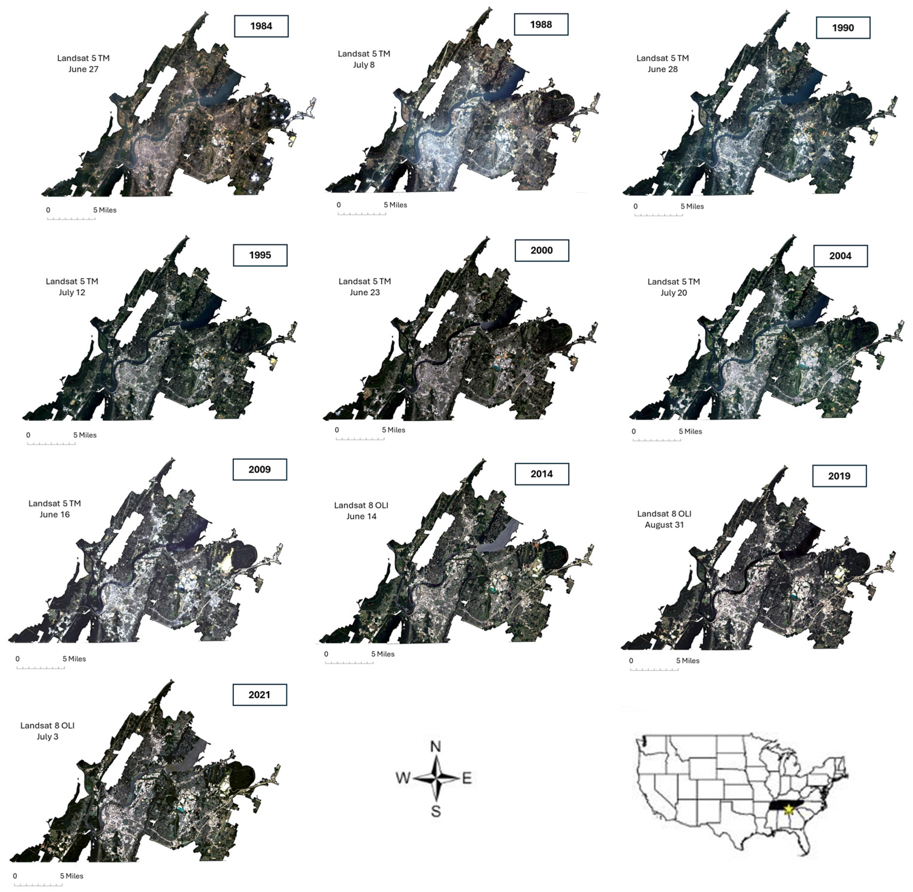
2.1. Study Site and Data Collection
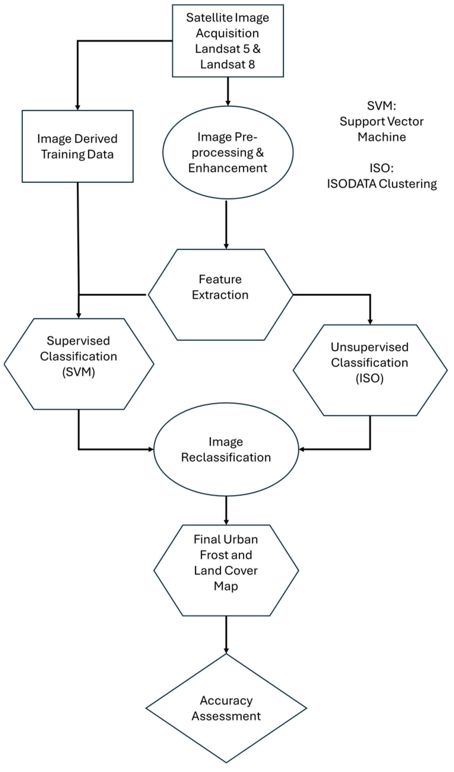
2.2. Data Processing
2.2.1. Image Pre-Processing and Enhancement
2.2.2. Feature Extraction
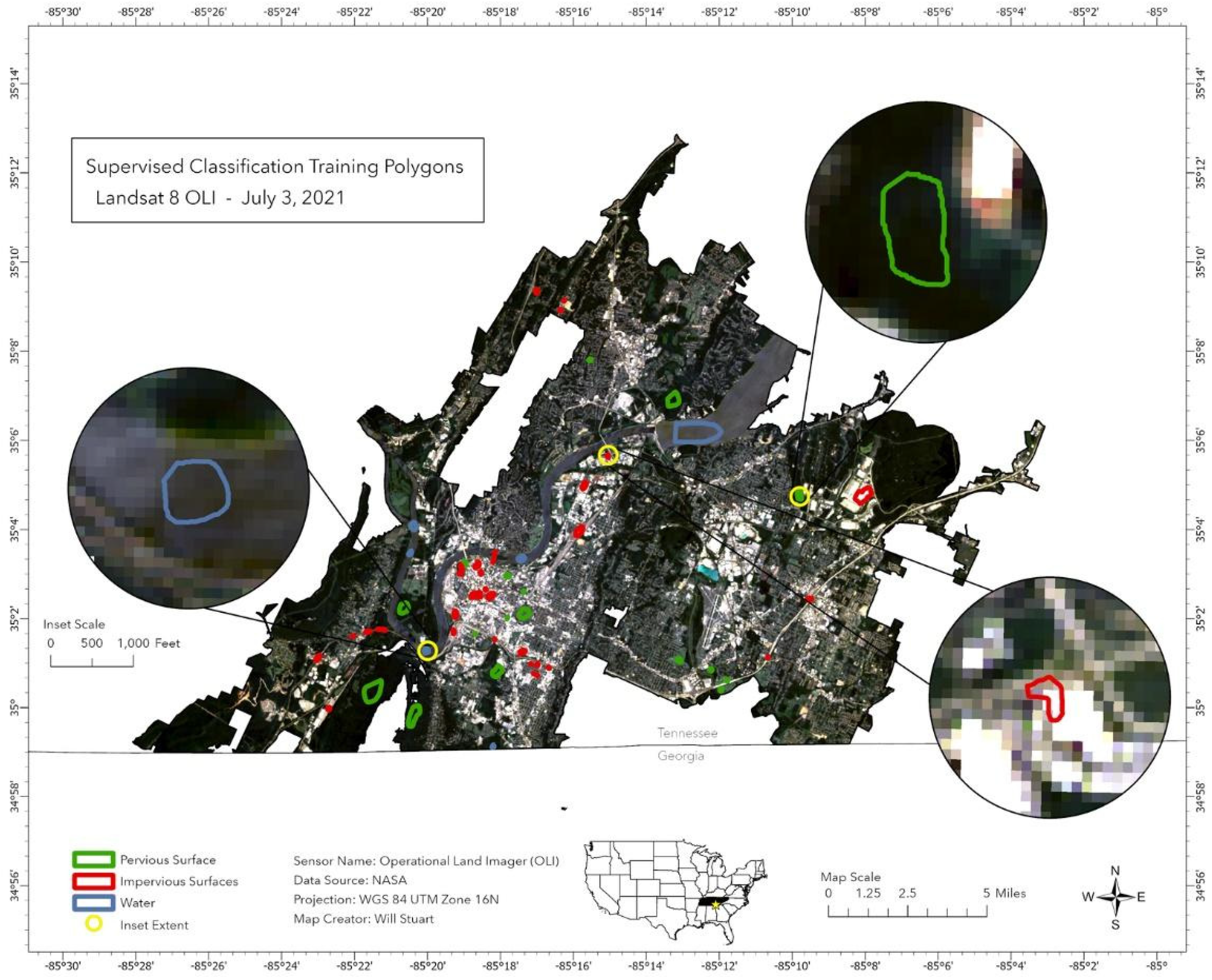
2.2.3. Supervised Classification
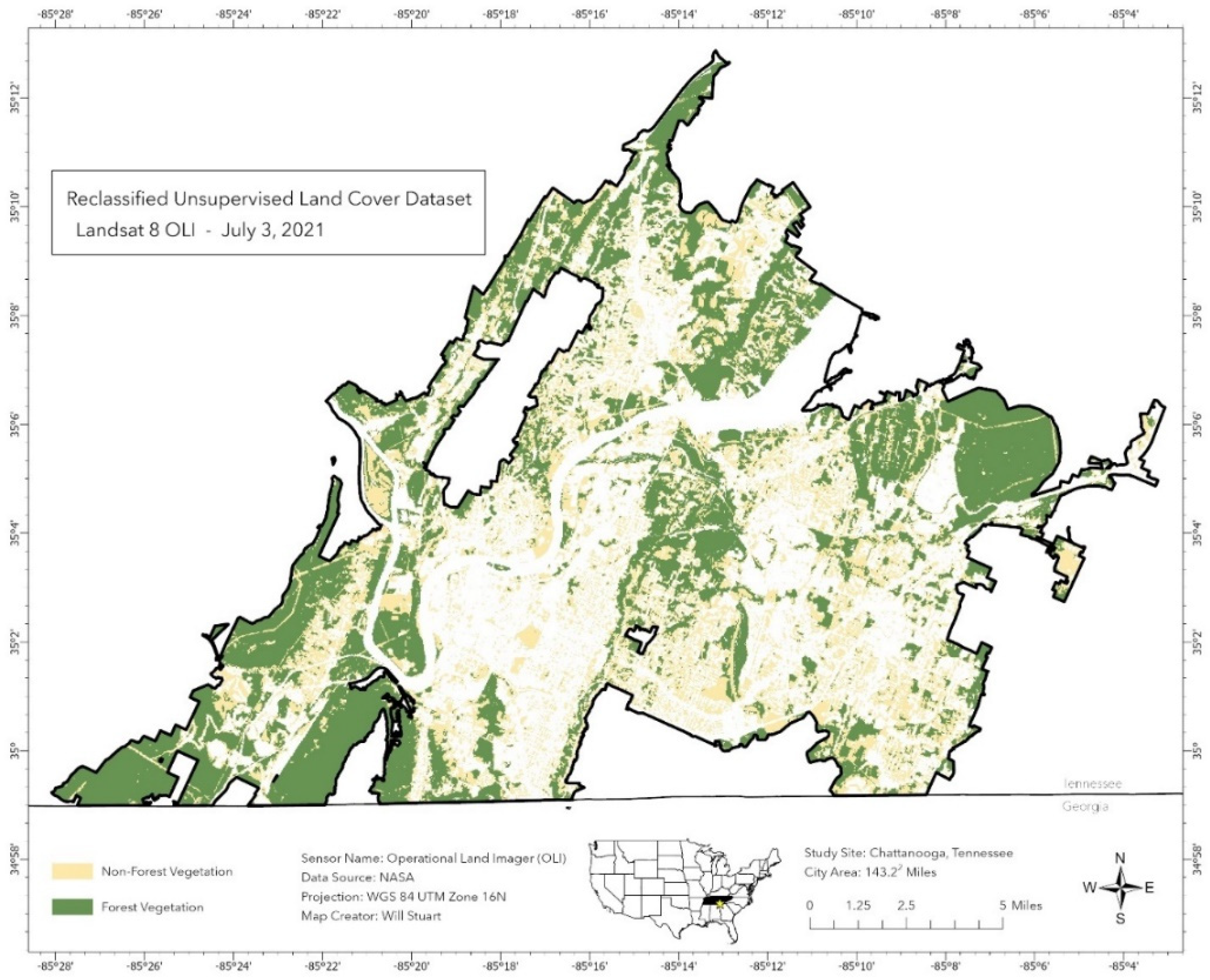
2.2.4. Unsupervised Classification
2.2.5. Post Processing—Image Reclassification

2.3. Data Analysis
2.4. Accuracy Assessment
3. Results and Analysis
3.1. Quantification of Land Cover Classes
3.2. Assessment of Spatiotemporal Trends
3.3. Accuracy Assessment
4. Discussion
5. Conclusions
Author Contributions
Funding
Data Availability Statement
Acknowledgments
Conflicts of Interest
References
- Reich, P.B.; Bolstad, P. Productivity of Evergreen and Deciduous Temperate Forests. Terrestrial Global Productivity; Academic Press: San Diego, CA, USA, 2001; pp. 245–283. [Google Scholar]
- Malhi, Y.A.; Baldocchi, D.; Jarvis, P. The carbon balance of tropical, temperate, and boreal forests. Plant Cell Environ. 1999, 22, 715–740. [Google Scholar] [CrossRef]
- Bundestag, D. Protecting the Tropical Forests: A High Priority Task; Woods-Schank, G., Translator; Deutscher Bundestag, Referat Öffentlichkeitsarbet: Bonn, Germany, 1990; p. 968. [Google Scholar]
- Heath, L.S.; Kauppi, P.E.; Burschel, P.; Gregor, H.D.; Guderian, R.; Kohlmaier, G.H.; Thomasius, H. Contribution of temperate forests to the world’s carbon budget. Water Air Soil Pollut. 1993, 70, 55–69. [Google Scholar] [CrossRef]
- Pan, Y.; Birdsey, R.A.; Phillips, O.L.; Jackson, R.B. The Structure, Distribution, and Biomass of the World’s Forests. Annu. Rev. Ecol. Evol. Syst. 2013, 44, 593–622. [Google Scholar] [CrossRef]
- FAO. Global Forest Resources Assessment 2020—Key Findings; Food and Agriculture Organization of the United Nations: Rome, Italy, 2020; p. 186. [Google Scholar]
- Kindermann, G.; Obersteiner, M.; Sohngen, B.; Sathaye, J.; Andrasko, K.; Rametsteiner, E.; Beach, R. Global cost estimates of reducing carbon emissions through avoided deforestation. Proc. Natl. Acad. Sci. USA 2008, 105, 10302–10307. [Google Scholar] [CrossRef]
- Lorenz, K.; Lal, R. Carbon Sequestration in Forest Ecosystems; Springer: Dordrecht, The Netherlands; Berlin/Heidelberg, Germany; London, UK; New York, NY, USA, 2009; p. 279. [Google Scholar]
- IPCC. Climate Change and Land: IPCC Special Report on Climate Change, Desertification, Land Degradation, Sustainable Land Management, Food Security, and Greenhouse Gas Fluxes in Terrestrial Ecosystems; Cambridge University Press: Cambridge, UK, 2022; pp. 1–36. [Google Scholar]
- Brandão, M.; Levasseur, A.; Kirschbaum, M.U.; Weidema, B.P.; Cowie, A.L.; Jørgensen, S.V. Key issues and options in accounting for carbon sequestration and temporary storage in life cycle assessment and carbon footprinting. Int. J. Life Cycle Assess. 2013, 18, 230–240. [Google Scholar] [CrossRef]
- Tans, P.P.; Fung, I.Y.; Akahashi, T. Observational constraints on the global atmospheric CO2 budget. Science 1990, 247, 1431–1438. [Google Scholar] [CrossRef]
- Schimel, D.S. Terrestrial ecosystems and the carbon cycle. Glob. Chang. Biol. 1995, 1, 77–91. [Google Scholar] [CrossRef]
- Spicer, M.E.; Mellor, H.; Carson, W.P. Seeing beyond the trees: A comparison of tropical and temperate plant growth forms and their vertical distribution. Ecology 2020, 101, e02974. [Google Scholar] [CrossRef]
- Seto, K.C.; Sánchez-Rodríguez, R.; Fragkias, M. The new geography of contemporary urbanization and the environment. Annu. Rev. Environ. Resour. 2010, 35, 167–194. [Google Scholar] [CrossRef]
- Hossain, A.; Stuart, W.; Mies, J.; Brock-Hon, A. Investigating Urban Heat Island (UHI) Impact for the City of Chattanooga, Tennessee Using GIS and Remote Sensing. In Handbook of Climate Change Mitigation and Adaptation; Lackner, M., Sajjadi, B., Chen, W.Y., Eds.; Springer: New York, NY, USA, 2021; pp. 1–35. [Google Scholar]
- Nowak, D.J.; Noble, M.H.; Sisinni, S.M.; Dwyer, J.F. People and trees: Assessing the US urban forest resource. J. For. 2001, 99, 37–42. [Google Scholar] [CrossRef]
- Nowak, D.J.; Hoehn, R.E.; Bodine, A.R.; Greenfield, E.J.; O’Neil-Dunne, J. Urban forest structure, ecosystem services and change in Syracuse, NY. Urban Ecosyst. 2016, 19, 1455–1477. [Google Scholar] [CrossRef]
- Endreny, T.A. Strategically growing the urban forest will improve our world. Nat. Commun. 2018, 9, 1–3. [Google Scholar] [CrossRef]
- Nowak, D.J.; Greenfield, E.J. US urban forest statistics, values, and projections. J. For. 2018, 116, 164–177. [Google Scholar] [CrossRef]
- Fornal-Pieniak, B.; Ollik, M.; Schwerk, A. Impact of different levels of anthropogenic pressure on the plant species composition in woodland sites. Urban For. Urban Green. 2019, 38, 295–304. [Google Scholar] [CrossRef]
- Aryal, P.C.; Aryal, C.; Bhusal, K.; Chapagain, D.; Dhamala, M.K.; Maharjan, S.R. Forest structure and anthropogenic disturbances regulate plant invasion in urban forests. Urban Ecosyst. 2022, 25, 367–377. [Google Scholar] [CrossRef]
- Nowak, D.J.; Dwyer, J.F. Understanding the Benefits and Costs of Urban Forest Ecosystems. In Urban and Community Forestry in the Northeast; Kuser, J.E., Ed.; Springer: Dordrecht, The Netherlands, 2007; pp. 25–46. [Google Scholar]
- Davis, K.L. The Role of Sense of Place: A Theoretical Framework to Aid Urban Forest Decision-Making. Ph.D. Thesis, The University of Tennessee, Knoxville, TN, USA, 2011. [Google Scholar]
- Livesley, S.; McPherson, E.G.; Calfapietra, C. The urban forest and ecosystem services: Impacts on urban water, heat, and pollution cycles at the tree, street, and city scale. J. Environ. Qual. 2016, 45, 119–124. [Google Scholar] [CrossRef]
- Albiero-Júnior, A.; Venegas-González, A.; Rodríguez-Catón, M.; Oliveira, J.M.; Longhi-Santos, T.; Galvão, F.; Botosso, P.C. Edge effects modify the growth dynamics and climate sensitivity of Araucaria angustifolia trees. Tree-Ring Res. 2020, 76, 11–26. [Google Scholar] [CrossRef]
- Morreale, L.L.; Thompson, J.R.; Tang, X.; Reinmann, A.B.; Hutyra, L.R. Elevated growth and biomass along temperate forest edges. Nat. Commun. 2021, 12, 1–8. [Google Scholar]
- Garvey, S.M.; Templer, P.H.; Pierce, E.A.; Reinmann, A.B.; Hutyra, L.R. Diverging patterns at the forest edge: Soil respiration dynamics of fragmented forests in urban and rural areas. Glob. Chang. Biol. 2022, 28, 3094–3109. [Google Scholar] [CrossRef]
- Muukkonen, P.; Heiskanen, J. Biomass estimation over a large area based on standwise forest inventory data and ASTER and MODIS satellite data: A possibility to verify carbon inventories. Remote Sens. Environ. 2007, 107, 617–624. [Google Scholar] [CrossRef]
- Li, B.; Xu, X.; Zhang, L.; Han, J.; Bian, C.; Li, G.; Jin, L. Above-ground biomass estimation and yield prediction in potato by using UAV-based RGB and hyperspectral imaging. ISPRS J. Photogramm. Remote Sens. 2020, 162, 161–172. [Google Scholar] [CrossRef]
- Alrababah, M.A.; Alhamad, M.N.; Bataineh, A.L.; Bataineh, M.M.; Suwaileh, A.F. Estimating east Mediterranean forest parameters using Landsat ETM. Int. J. Remote Sens. 2011, 32, 1561–1574. [Google Scholar] [CrossRef]
- Castillo, J.A.A.; Apan, A.A.; Maraseni, T.N.; Salmo III, S.G. Estimation and mapping of above-ground biomass of mangrove forests and their replacement land uses in the Philippines using Sentinel imagery. ISPRS J. Photogramm. Remote Sens. 2017, 134, 70–85. [Google Scholar] [CrossRef]
- Duncan, J.M.A.; Boruff, B.; Saunders, A.; Sun, Q.; Hurley, J.; Amati, M. Turning down the heat: An enhanced understanding of the relationship between urban vegetation and surface temperature at the city scale. Sci. Total Environ. 2019, 656, 118–128. [Google Scholar] [CrossRef]
- Zhang, L.; Shao, Z.; Liu, J.; Cheng, Q. Deep learning based retrieval of forest aboveground biomass from combined LiDAR and Landsat 8 data. Remote Sens. 2019, 11, 1459. [Google Scholar] [CrossRef]
- Jensen, J.R. Remote Sensing of the Environment: An Earth Resource Perspective; Pearson Prentice Hall: Hoboken, NJ, USA, 2007; p. 544. [Google Scholar]
- Bourgoin, C.; Blanc, L.; Bailly, J.S.; Cornu, G.; Berenguer, E.; Oszwald, J.; Gond, V. The potential of multisource remote sensing for mapping the biomass of a degraded Amazonian forest. Forests 2018, 9, 303. [Google Scholar] [CrossRef]
- Foody, G.M.; Boyd, D.S.; Cutler, M.E. Predictive relations of tropical forest biomass from Landsat TM data and their transferability between regions. Remote Sens. Environ. 2003, 85, 463–474. [Google Scholar] [CrossRef]
- Cohen, W.B.; Maiersperger, T.K.; Gower, S.T.; Turner, D.P. An improved strategy for regression of biophysical variables and Landsat ETM+ data. Remote Sens. Environ. 2003, 84, 561–571. [Google Scholar] [CrossRef]
- Frazier, R.J.; Coops, N.C.; Wulder, M.A.; Kennedy, R. Characterization of aboveground biomass in an unmanaged boreal forest using Landsat temporal segmentation metrics. ISPRS J. Photogramm. Remote Sens. 2014, 92, 137–146. [Google Scholar] [CrossRef]
- Gómez, C.; White, J.C.; Wulder, M.A.; Alejandro, P. Historical forest biomass dynamics modelled with Landsat spectral trajectories. ISPRS J. Photogramm. Remote Sens. 2014, 93, 14–28. [Google Scholar] [CrossRef]
- Tian, X.; Li, Z.; Su, Z.; Chen, E.; van der Tol, C.; Li, X.; Ling, F. Estimating montane forest above-ground biomass in the upper reaches of the Heihe River Basin using Landsat-TM data. Int. J. Remote Sens. 2014, 35, 7339–7362. [Google Scholar] [CrossRef]
- Gu, C.; Clevers, J.G.; Liu, X.; Tian, X.; Li, Z.; Li, Z. Predicting forest height using the GOST, Landsat 7 ETM+, and airborne LiDAR for sloping terrains in the Greater Khingan Mountains of China. ISPRS J. Photogramm. Remote Sens. 2018, 137, 97–111. [Google Scholar] [CrossRef]
- Izadi, S.; Sohrabi, H.; Khaledi, M.J. Estimation of coppice forest characteristics using spatial and non-spatial models and Landsat data. J. Spat. Sci. 2020, 67, 143–156. [Google Scholar] [CrossRef]
- Jenner, L. Landsat Overview. Available online: https://www.nasa.gov/mission_pages/landsat/overview/index.html (accessed on 27 October 2020).
- Blanton, R.; Hossain, A. Mapping the Recovery Process of Vegetation Growth in the Copper Basin, Tennessee Using Remote Sensing Technology. GeoHazards 2020, 1, 31–43. [Google Scholar] [CrossRef]
- Hall, J.; Hossain, A. Mapping urbanization and evaluating its possible impacts on stream water quality in Chattanooga, Tennessee, using GIS and remote sensing. Sustainability 2020, 12, 1980. [Google Scholar] [CrossRef]
- Jensen, J.R. Introductory Digital Image Processing: A Remote Sensing Perspective; Prentice-Hall: Upper Saddle River, NJ, USA, 2015; pp. 1–544. [Google Scholar]
- Stuart, W. Mapping Urban Forest Extent and Modeling Sequestered Carbon Across Chattanooga, Tennessee’s Urban Forest Canopy Using GIS and Remote Sensing Principles. Unpublished Thesis, The University of Tennessee at Chattanooga, Chattanooga, TN, USA, 2023. [Google Scholar]
- Lillesand, T.M.; Kiefer, R.W. Remote Sensing and Image Interpretation; John Willey and Sons, Inc.: Hoboken, NJ, USA, 2000; pp. 1–724. [Google Scholar]
- Townshend, J.R.G. Land cover. Int. J. Remote Sens. 1992, 13, 1319–1328. [Google Scholar] [CrossRef]
- Lu, D.; Weng, Q. A survey of image classification methods and techniques for improving classification performance. Int. J. Remote Sens. 2007, 28, 823–870. [Google Scholar] [CrossRef]
- Srivastava, P.K.; Kiran, G.; Gupta, M.; Sharma, N.; Prasad, K. A study on distribution of heavy metal contamination in vegetables using GIS and analytical technique. Int. J. Ecol. Dev. 2012, 21, 89–99. [Google Scholar]
- Kavzoglu, T.; Reis, S. Performance analysis of maximum likelihood and artificial neural network classifiers for training sets with mixed pixels. GIScience Remote Sens. 2008, 45, 330–342. [Google Scholar] [CrossRef]
- Szuster, B.W.; Chen, Q.; Borger, M. A comparison of classification techniques to support land cover and landuse analysis in tropical coastal zones. Appl. Geogr. 2011, 31, 525–532. [Google Scholar] [CrossRef]
- Yu, L.; Porwal, A.; Holden, E.J.; Dentith, M.C. Towards automatic lithological classification from remote sensing data using support vector machines. Comput. Geosci. 2021, 45, 229–239. [Google Scholar] [CrossRef]
- Vapnik, V.N. The Nature of Statistical Learning Theory; Springer: New York, NY, USA, 1995; pp. 1–334. [Google Scholar]
- Kavzoglu, T.; Colkesen, I. A kernel functions analysis for support vector machines for land cover classification. Int. J. Appl. Earth Obs. Geoinf. 2009, 11, 352–359. [Google Scholar] [CrossRef]
- Fitzgerald, R.; Lees, B. Assessing the classification accuracy of multisource remote sensing data. Remote Sens. Environ. 1994, 47, 362–368. [Google Scholar] [CrossRef]
- Masson, L.F.; MCNeill, G.; Tomany, J.; Simpson, J.; Peace, H.S.; Wei, L.; Grubb, D.; Bolton-Smith, C. Statistical approaches for assessing the relative validity of a food-frequency questionnaire: Use of correlation coefficients and the kappa statistic. Public Health Nutr. 2003, 6, 313–321. [Google Scholar] [CrossRef]
- Reed, J.A.; Ainsworth, B.E.; Wilson, D.K.; Mixon, G.; Cook, A. Awareness and use of community walking trails. Prev. Med. 2004, 39, 903–908. [Google Scholar] [CrossRef]
- Cofer, B. Gross to Green: City Makes Strides to Becoming Sustainable; The Times Free Press: Chattanooga, TN, USA, 2011. [Google Scholar]
- Sohn, P. Chattanooga Creek Still Threatened; The Times Free Press: Chattanooga, TN, USA, 2010. [Google Scholar]


| Bands | Description | Wavelength (μm) | Spatial Resolution (m) | Temporal Resolution | |
|---|---|---|---|---|---|
| Landsat 5 | TM 1 | Blue | 0.45–0.52 | 30 | 16 Days |
| TM 2 | Green | 0.52–0.60 | 30 | ||
| TM 3 | Red | 0.63–0.69 | 30 | ||
| TM 4 | Near-Infrared | 0.76–0.90 | 30 | ||
| TM 5 | Near-Infrared | 1.55–1.75 | 30 | ||
| TM 6 | Thermal-Infrared | 10.40–12.50 | 120 | ||
| TM 7 | Mid-Infrared | 2.08–2.35 | 30 | ||
| Landsat 8 | OLI 1 | Coastal Aerosol | 0.43–0.45 | 30 | 16 Days |
| OLI 2 | Blue | 0.45–0.51 | 30 | ||
| OLI 3 | Green | 0.53–0.59 | 30 | ||
| OLI 4 | Red | 0.64–0.67 | 30 | ||
| OLI 5 | Near-Infrared | 0.85–0.88 | 30 | ||
| OLI 6 | Shortwave-Infrared | 1.57–1.65 | 30 | ||
| OLI 7 | Shortwave-Infrared | 2.11–2.29 | 30 | ||
| OLI 8 | Panchromatic | 0.50–0.68 | 15 | ||
| OLI 9 | Cirrus | 1.36–1.38 | 30 |
| Scene ID | Year | Month and Day | Acquisition Gap | Satellite–Sensor | RGB |
|---|---|---|---|---|---|
| 1 | 1984 | June 27 | 0 | Landsat 5—TM | 321 |
| 2 | 1988 | July 8 | 4 | 321 | |
| 3 | 1990 | June 28 | 2 | 321 | |
| 4 | 1995 | July 12 | 5 | 321 | |
| 5 | 2000 | June 23 | 5 | 321 | |
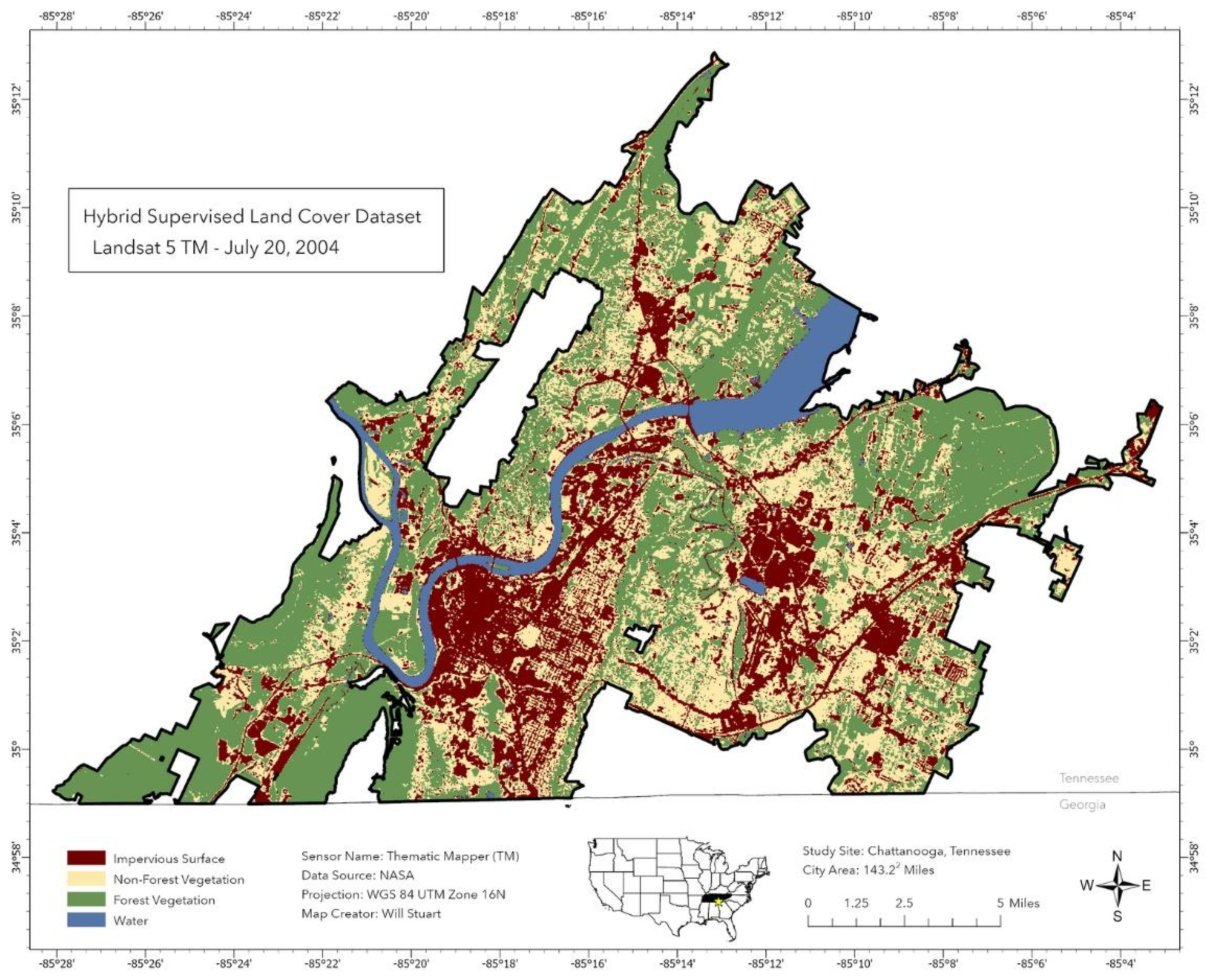
| 6 | 2004 | July 20 | 4 | 321 | |
| 7 | 2009 | June 16 | 5 | 321 | |
| 8 | 2014 | June 14 | 5 | Landsat 8—OLI | 432 |
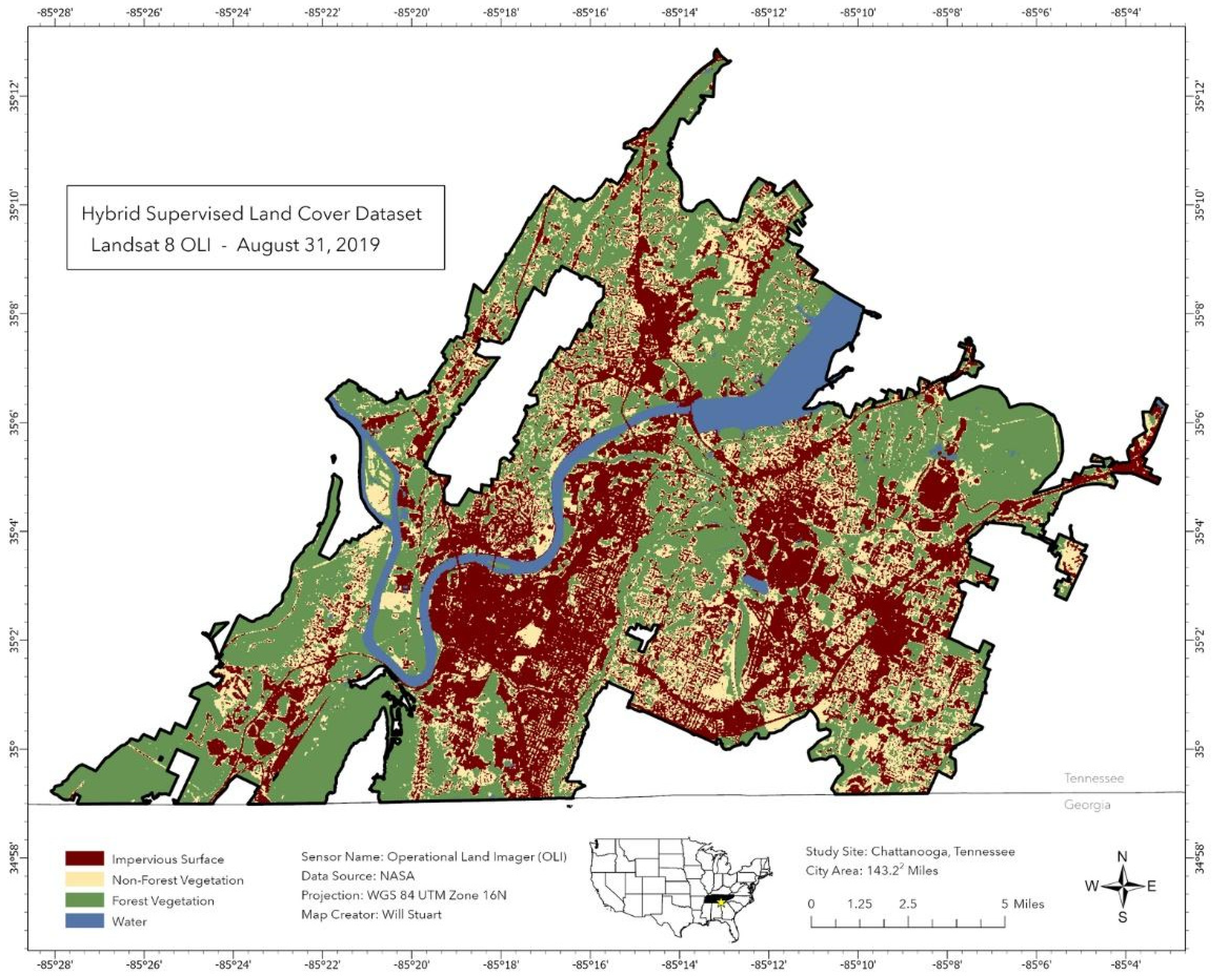
| 9 | 2019 | August 31 | 6 | 432 | |
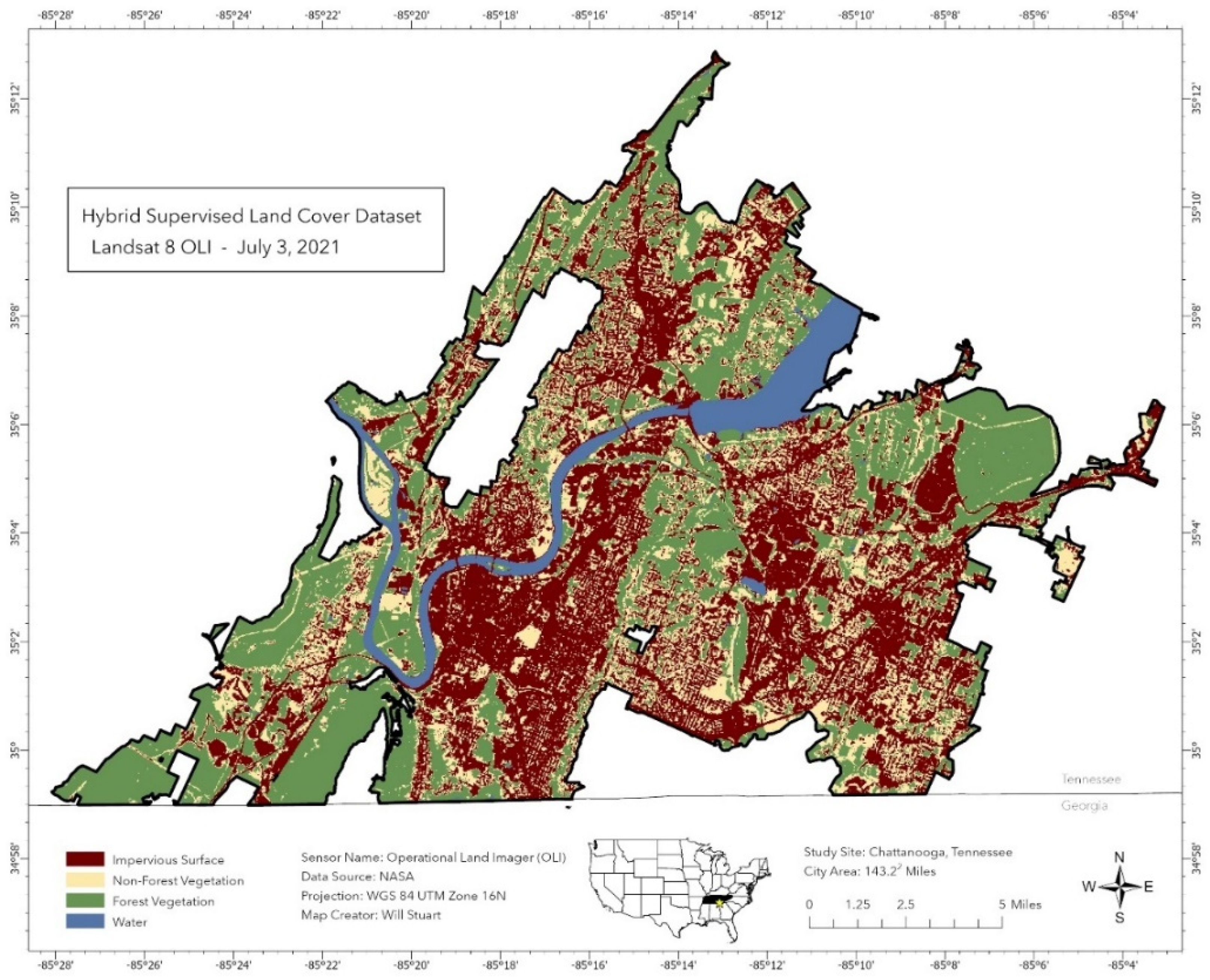
| 10 | 2021 | July 3 | 1 | 432 |
| Land Class | Class Code | Class Description |
|---|---|---|
| Impervious Surfaces | 1 | Buildings, Roads, Cars, Parking Lots, Artificial Turf, etc. |
| Non-Forest Vegetation | 2 | Grasses, Scrubs, Shrubs, Crops, Ornamental Plants, etc. |
| Urban Forest Canopy | 3 | All tree canopy within the study area. |
| Water | 4 | Flooded Wetlands, Rivers, Streams, Man-Made Retention Ponds, etc. |
| Impervious Surface | NF Vegetation | Forest Canopy | Water | |||||
|---|---|---|---|---|---|---|---|---|
| Acres | % Area | Acres | % Area | Acres | % Area | Acres | % Area | |
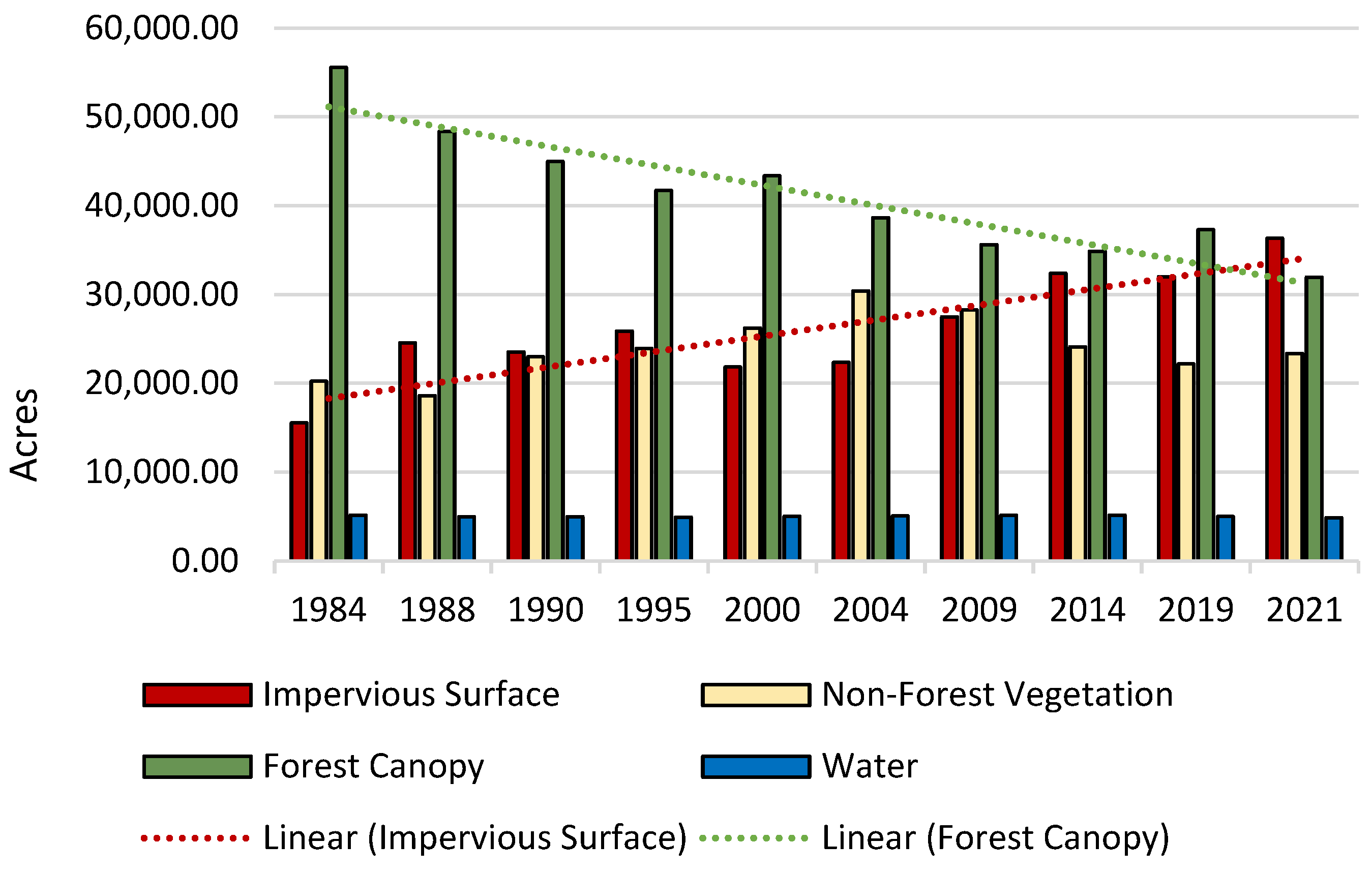
| 1984 | 15,526 | 16.10% | 20,229 | 20.97% | 55,549 | 57.60% | 5140 | 5.33% |
| 1988 | 24,546 | 25.45% | 18,595 | 19.28% | 48,325 | 50.11% | 4979 | 5.16% |
| 1990 | 23,512 | 24.38% | 22,976 | 23.82% | 44,968 | 46.63% | 4988 | 5.17% |
| 1995 | 25,875 | 26.83% | 23,931 | 24.81% | 41,707 | 43.24% | 4931 | 5.11% |
| 2000 | 21,833 | 22.64% | 26,213 | 27.18% | 43,356 | 44.95% | 5043 | 5.23% |
| 2004 | 22,358 | 23.18% | 30,393 | 31.51% | 38,630 | 40.05% | 5063 | 5.25% |
| 2009 | 27,485 | 28.50% | 28,235 | 29.28% | 35,590 | 36.90% | 5134 | 5.32% |
| 2014 | 32,365 | 33.56% | 24,086 | 24.97% | 34,857 | 36.14% | 5136 | 5.33% |
| 2019 | 31,981 | 33.16% | 22,188 | 23.01% | 37,278 | 38.65% | 4991 | 5.18% |
| 2021 | 36,316 | 37.65% | 23,347 | 24.21% | 31,924 | 33.10% | 4857 | 5.04% |
| Impervious Surface | Non-Forest Vegetation | Forest Canopy | Water | |
|---|---|---|---|---|
| 1984–1988 | 58.09% | −8.08% | −13.01% | −3.13% |
| 1988–1990 | −4.21% | 23.56% | −6.95% | 0.19% |
| 1990–1995 | 10.05% | 4.16% | −7.25% | −1.15% |
| 1995–2000 | −15.62% | 9.53% | 3.95% | 2.27% |
| 2000–2004 | 2.40% | 15.95% | −10.90% | 0.40% |
| 2004–2009 | 22.93% | −7.10% | −7.87% | 1.41% |
| 2009–2014 | 17.75% | −14.69% | −2.06% | 0.04% |
| 2014–2019 | −1.19% | −7.88% | 6.94% | −2.83% |
| 2019–2021 | 13.55% | 5.23% | −14.36% | −2.68% |
| Classified Pixels | Developed | Non-Forest Vegetation | Forest | Water | Total (Classified) | User’s Accuracy | |
| 1984 | Developed Pixels | 413 | 18 | 2 | 0 | 433 | 95.38% |
| Non-Forest Vegetation Pixels | 166 | 206 | 135 | 0 | 507 | 40.63% | |
| Forest Pixels | 0 | 0 | 1026 | 0 | 1026 | 100.00% | |
| Water Pixels | 0 | 0 | 0 | 2599 | 2599 | 100.00% | |
| Total (Reference) | 579 | 224 | 1163 | 2599 | 4565 | ||
| Producer’s Accuracy | 71.33% | 91.96% | 88.22% | 100.00% | Overall = 92.97% | ||
| Classified Pixels | Developed | Non-Forest Vegetation | Forest | Water | Total (Classified) | User’s Accuracy | |
| 1988 | Developed Pixels | 214 | 3 | 3 | 0 | 220 | 97.27% |
| Non-Forest Vegetation Pixels | 66 | 172 | 60 | 0 | 298 | 57.72% | |
| Forest Pixels | 22 | 28 | 709 | 0 | 759 | 93.41% | |
| Water Pixels | 0 | 0 | 0 | 2599 | 2599 | 100.00% | |
| Total (Reference) | 302 | 203 | 772 | 2599 | 3876 | ||
| Producer’s Accuracy | 70.86% | 84.73% | 91.84% | 100.00% | Overall = 95.30% | ||
| Classified Pixels | Developed | Non-Forest Vegetation | Forest | Water | Total (Classified) | User’s Accuracy | |
| 1990 | Developed Pixels | 206 | 0 | 0 | 0 | 206 | 100.00% |
| Non-Forest Vegetation Pixels | 102 | 263 | 6 | 0 | 371 | 70.89% | |
| Forest Pixels | 0 | 0 | 802 | 0 | 802 | 100.00% | |
| Water Pixels | 0 | 1 | 1 | 2597 | 2599 | 99.92% | |
| Total (Reference) | 308 | 264 | 809 | 2597 | 3978 | ||
| Producer’s Accuracy | 66.88% | 99.62% | 99.13% | 100.00% | Overall = 97.23% | ||
| Classified Pixels | Developed | Non-Forest Vegetation | Forest | Water | Total (Classified) | User’s Accuracy | |
| 1995 | Developed Pixels | 157 | 0 | 0 | 0 | 157 | 100.00% |
| Non-Forest Vegetation Pixels | 2 | 294 | 43 | 0 | 339 | 86.73% | |
| Forest Pixels | 0 | 0 | 431 | 0 | 431 | 100.00% | |
| Water Pixels | 0 | 0 | 0 | 2599 | 2599 | 100.00% | |
| Total (Reference) | 159 | 294 | 474 | 2599 | 3526 | ||
| Producer’s Accuracy | 98.74% | 100.00% | 90.93% | 100.00% | Overall = 98.72% | ||
| Classified Pixels | Developed | Non-Forest Vegetation | Forest | Water | Total (Classified) | User’s Accuracy | |
| 2000 | Developed Pixels | 132 | 0 | 0 | 0 | 132 | 100.00% |
| Non-Forest Vegetation Pixels | 0 | 164 | 149 | 0 | 313 | 52.40% | |
| Forest Pixels | 41 | 0 | 606 | 0 | 647 | 93.66% | |
| Water Pixels | 0 | 0 | 0 | 2599 | 2599 | 100.00% | |
| Total (Reference) | 173 | 164 | 755 | 2599 | 3691 | ||
| Producer’s Accuracy | 76.30% | 100.00% | 80.26% | 100.00% | Overall = 94.85% |
| Classified Pixels | Developed | Non-Forest Vegetation | Forest | Water | Total (Classified) | User’s Accuracy | |
| 2004 | Developed Pixels | 125 | 0 | 0 | 0 | 125 | 100.00% |
| Non-Forest Vegetation pixels | 51 | 187 | 0 | 0 | 238 | 78.57% | |
| Forest Pixels | 0 | 1 | 417 | 0 | 418 | 99.76% | |
| Water Pixels | 0 | 0 | 0 | 2599 | 2599 | 100.00% | |
| Total (Reference) | 176 | 188 | 417 | 2599 | 3380 | ||
| Producer’s Accuracy | 71.02% | 99.47% | 100.00% | 100.00% | Overall = 98.46% | ||
| Classified Pixels | Developed | Non-Forest Vegetation | Forest | Water | Total (Classified) | User’s Accuracy | |
| 2009 | Developed Pixels | 295 | 0 | 0 | 0 | 295 | 100.00% |
| Non-Forest Vegetation Pixels | 24 | 159 | 10 | 0 | 193 | 82.38% | |
| Forest Pixels | 0 | 0 | 1658 | 0 | 1658 | 100.00% | |
| Water Pixels | 0 | 0 | 0 | 2599 | 2599 | 100.00% | |
| Total (Reference) | 319 | 159 | 1668 | 2599 | 4745 | ||
| Producer’s Accuracy | 92.48% | 100.00% | 99.40% | 100.00% | Overall = 99.28% | ||
| Classified Pixels | Developed | Non-Forest Vegetation | Forest | Water | Total (Classified) | User’s Accuracy | |
| 2014 | Developed Pixels | 297 | 0 | 0 | 0 | 297 | 100.00% |
| Non-Forest Vegetation Pixels | 46 | 161 | 5 | 0 | 212 | 75.94% | |
| Forest Pixels | 1 | 0 | 1190 | 0 | 1191 | 99.92% | |
| Water Pixels | 0 | 0 | 0 | 2599 | 2599 | 100.00% | |
| Total (Reference) | 344 | 161 | 1195 | 2599 | 4299 | ||
| Producer’s Accuracy | 86.34% | 100.00% | 99.58% | 100.00% | Overall = 98.79% | ||
| Classified Pixels | Developed | Non-Forest Vegetation | Forest | Water | Total (Classified) | User’s Accuracy | |
| 2019 | Developed Pixels | 253 | 0 | 0 | 0 | 253 | 100.00% |
| Non-Forest Vegetation Pixels | 15 | 152 | 6 | 0 | 173 | 87.86% | |
| Forest Pixels | 0 | 8 | 1288 | 0 | 1296 | 99.38% | |
| Water Pixels | 0 | 0 | 0 | 2599 | 2599 | 100.00% | |
| Total (Reference) | 268 | 160 | 1294 | 2599 | 4321 | ||
| Producer’s Accuracy | 94.40% | 95.00% | 99.54% | 100.00% | Overall = 99.33% | ||
| Classified Pixels | Developed | Non-Forest Vegetation | Forest | Water | Total (Classified) | User’s Accuracy | |
| 2021 | Developed Pixels | 586 | 1 | 0 | 0 | 587 | 99.83% |
| Non-Forest Vegetation Pixels | 3 | 302 | 0 | 0 | 305 | 99.02% | |
| Forest Pixels | 0 | 13 | 2431 | 0 | 2444 | 99.47% | |
| Water Pixels | 0 | 0 | 0 | 2599 | 2599 | 100.00% | |
| Total (Reference) | 589 | 316 | 2431 | 2599 | 5935 | ||
| Producer’s Accuracy | 99.49% | 95.57% | 100.00% | 100.00% | Overall = 99.71% |
Disclaimer/Publisher’s Note: The statements, opinions and data contained in all publications are solely those of the individual author(s) and contributor(s) and not of MDPI and/or the editor(s). MDPI and/or the editor(s) disclaim responsibility for any injury to people or property resulting from any ideas, methods, instructions or products referred to in the content. |
© 2024 by the authors. Licensee MDPI, Basel, Switzerland. This article is an open access article distributed under the terms and conditions of the Creative Commons Attribution (CC BY) license (https://creativecommons.org/licenses/by/4.0/).
Share and Cite
Stuart, W.; Hossain, A.K.M.A.; Hunt, N.; Mix, C.; Qin, H. Spatiotemporal Analysis of Urban Forest in Chattanooga, Tennessee from 1984 to 2021 Using Landsat Satellite Imagery. Remote Sens. 2024, 16, 2419. https://doi.org/10.3390/rs16132419
Stuart W, Hossain AKMA, Hunt N, Mix C, Qin H. Spatiotemporal Analysis of Urban Forest in Chattanooga, Tennessee from 1984 to 2021 Using Landsat Satellite Imagery. Remote Sensing. 2024; 16(13):2419. https://doi.org/10.3390/rs16132419
Chicago/Turabian StyleStuart, William, A. K. M. Azad Hossain, Nyssa Hunt, Charles Mix, and Hong Qin. 2024. "Spatiotemporal Analysis of Urban Forest in Chattanooga, Tennessee from 1984 to 2021 Using Landsat Satellite Imagery" Remote Sensing 16, no. 13: 2419. https://doi.org/10.3390/rs16132419