Abstract
Potential inconsistencies between the goals of unsupervised representation learning and clustering within multi-stage deep clustering can diminish the effectiveness of these techniques. However, because the goal of unsupervised representation learning is inherently flexible and can be tailored to clustering, we introduce PointStaClu, a novel single-stage point cloud clustering method. This method employs stable cluster discrimination (StaClu) to tackle the inherent instability present in single-stage deep clustering training. It achieves this by constraining the gradient descent updates for negative instances within the cross-entropy loss function, and by updating the cluster centers using the same loss function. Furthermore, we integrate entropy constraints to regulate the distribution entropy of the dataset, thereby enhancing the cluster allocation. Our framework simplifies the process, employing a single loss function and an encoder for deep point cloud clustering. Extensive experiments on the ModelNet40 and ShapeNet dataset demonstrate that PointStaClu significantly narrows the performance gap between unsupervised point cloud clustering and supervised point cloud classification, presenting a novel approach to point cloud classification tasks.
1. Introduction
With the advancement of 3D acquisition technology, obtaining large volumes of 3D data—like grids, point clouds, and depth images—has become increasingly straightforward [1,2,3]. These data provide a more realistic and natural representation of objects and environments, surpassing the capabilities of traditional 2D images. Consequently, it has garnered significant attention in burgeoning sectors such as autonomous driving, robotics, and virtual reality, thereby accelerating the growth of research in point cloud processing. Among the various applications of point cloud analysis, classification emerges as a key challenge. It involves assigning predefined semantic labels to the complex and diverse data points within point clouds (e.g., aircraft, tables, lights, etc.).
The rapid evolution of deep neural networks (DNNs) has significantly advanced point cloud processing [4,5,6]. Earlier pioneering works, such as PointNet [7], applied neural networks directly to process discrete and irregular point cloud data for tasks like classification and segmentation. This has ignited extensive research into analyzing 3D point clouds using DNNs. Recent developments in neural networks for raw 3D point cloud data have further advanced the various point cloud processing tasks. However, the manual annotation of datasets is often time consuming [8,9,10], laborious, and prone to errors. Moreover, models trained on manually labeled data may exhibit limited generalization capabilities. Therefore, there is an urgent need for neural networks that can autonomously learn the distinctive feature representations of point clouds and cluster them into semantically meaningful groups without human intervention.
Unsupervised representation learning in point clouds is extensively studied regarding its capability to learn distinctive feature representations without relying on labeled data [11,12,13]. Clustering, a fundamental task in unsupervised learning, involves partitioning an unlabeled dataset into clusters based on instance characteristics, with similar instances within the same cluster determined by a distance function [14]. Clustering algorithms, including k-means [15] and subspace clustering, generally concentrate on identifying suitable distance metrics and developing efficient algorithms for established features. Although depth image clustering methods provide flexibility in capturing data distribution and learning representations, they may occasionally result in the convergence of all instances into a single feature [16]. To address this issue, researchers are investigating multi-stage training strategies that decouple representation learning from clustering. Studies indicate that pre-training on extensive unlabeled datasets can generate rich features that capture semantic similarities without collapsing [17,18,19]. Multi-stage deep image clustering methodologies begin with an unsupervised representation learning phase, followed by a model enhancement stage aimed at bolstering the clustering efficacy. In contrast, single-stage clustering techniques produce definitive clustering outcomes from initial data in a single computational pass, avoiding the need for preliminary training or subsequent refinements, thus enabling rapid data aggregation with straightforward efficiency. Multi-stage methodologies outperform their single-stage counterparts by utilizing the optimized proximities from the pre-training phase to enhance the clustering precision.
Although multi-stage clustering methods show promise, they encounter challenges. The optimization in these methods is more intricate compared to current end-to-end learning approaches. Moreover, the goals of phased unsupervised representation learning may conflict with the clustering objectives, potentially impeding the deep clustering performance. The objective of unsupervised representation learning is arbitrary and depends on the pretext task selected, which might encompass reconstruction generation [20,21,22], instance identification [23,24], mask modeling [25,26,27], and so on. Many multi-stage methods pre-train with instance discrimination, aiming to uniquely categorize each instance, contrasting with clustering’s aim to group similar instances. To tackle this issue, SwAV [28] has been proposed and demonstrated that clustering can serve as an effective pretext task for unsupervised representation learning. Consequently, the focus should shift towards single-stage deep clustering strategies that simultaneously optimize representation and clustering, without the need for additional pretext tasks. Therefore, inspired by Secu [29], a single-stage depth image clustering method, we try to focus on single-stage depth point cloud clustering.
Deep clustering methods frequently employ cross-entropy losses to refine both the representations and the clustering centers. Cross-entropy loss is a commonly used metric in classification tasks, quantifying the difference between the predicted probabilities and actual outcomes. The core of this measure is to compare the model’s predicted probability distribution to the distribution of the true labels. This comparison is crucial for gauging the accuracy of the model’s predictions against reality. However, standard cross-entropy losses can be unstable in the context of single-stage clustering. This instability arises because the gradients that update the cluster centers include the contributions from both the relevant positive instances and irrelevant negative ones. Given the limited batch sizes typical in stochastic gradient descent (SGD), many clusters may not contain positive instances in each iteration, which can allow the influence of negative instances to dominate. Unlike supervised learning, which has static labels, cluster assignments in deep clustering are dynamic, evolving throughout the training process. As a result, the optimization process can become unstable due to the noise incrementally introduced by the high variance associated with negative instances.
To address the aforementioned issues, we introduce the PointStaClu method, based on stable clustering discrimination. This approach stabilizes single-stage deep clustering in unsupervised contexts by omitting the gradients of negative instances from the cross-entropy loss function that updates the cluster centers. Unlike k-means, which applies uniform weights to positive instances during cluster center updates, PointStaClu’s stable discriminant task adjusts weights according to the instance difficulty, placing greater emphasis on the challenging instances [30,31]. Furthermore, we incorporate an entropy constraint strategy to enhance the distribution of clusters within the dataset. Our framework streamlines deep point cloud clustering through a unified loss function and encoder. The key contributions of this work are as follows:
- We introduce PointStaClu, a point cloud clustering method that utilizes stable clustering discrimination, eliminating the need for additional pretext tasks. The stable cluster discrimination (StaClu) task bolsters the stability of single-stage deep clustering by omitting the gradients from the negative instances in the cross-entropy loss function responsible for updating cluster centers. It also adaptively assigns greater weight to challenging instances during the update process.
- We incorporate an entropy-constrained strategy to refine the distribution of clusters within the dataset.
- Our framework for deep point cloud clustering is streamlined, employing a single loss function and encoder.
2. Related Work
In this section, we provide a concise overview of the recent progress in two interconnected domains: unsupervised representation learning and deep clustering.
2.1. Unsupervised Representation Learning
Unsupervised representation learning is gaining prominence, driven by the proliferation of real-world data and the prohibitive costs associated with large-scale manual annotation. Its goal is to extract the robust and generic features from unlabeled data, thereby facilitating the easier resolution of subsequent tasks. Traditional methods, such as autoencoders, generative adversarial networks (GANs), and autoregressive models, learn representations by reconstructing inputs [32,33,34]. However, these methods often overlook the local geometric details, focusing instead on the low-level data changes, potentially limiting their performance on tasks such as classification.
Recently, contrast learning has emerged as an effective strategy for unsupervised representation learning. It focuses on identifying the shared features among similar instances while distinguishing the differences among dissimilar ones. In contrast to generative learning, contrast learning operates at a higher, more abstract semantic level, which simplifies the model and optimization process, thereby enhancing the generalization capabilities. Liu et al. [35] proposed a strategy for 3D point cloud representation that incentivizes the network to produce consistent features for points within the same local shape region, and distinct features for the points from different regions or noise points, leveraging point discrimination learning.
Furthermore, masked autoencoder frameworks have been investigated for their utility in unsupervised pre-training. These frameworks employ the random masking of the point cloud, compelling the autoencoder to reconstruct the obscured regions. Zhang et al. [26] introduced Point-M2AE, a multi-scale masked autoencoder framework designed for hierarchical feature representation of 3D point clouds. In a separate study, Zhang et al. [27] capitalized on the 2D knowledge from pre-trained models to inform the learning of 3D point cloud features through their I2P-MAE model, thereby attaining state-of-the-art performance in 3D representation.
2.2. Deep Clustering
Acknowledging the limitations of the traditional clustering methods when dealing with high-dimensional data, deep clustering has emerged as a solution that simultaneously optimizes representation learning and the clustering process. Recent studies have underscored the importance of integrating representation learning with clustering techniques to address the complexities inherent in data challenges. Some researchers have concentrated on fortifying representation learning through the application of equilibrium entropy constraints, which ensure a balanced distribution of instances across clusters [36]. For example, SimCLR, developed by Chen et al. [37], employs case discrimination as a pretext task, categorizing each sample uniquely and utilizing data augmentation strategies during training. Conversely, SwAV [28] eschews pairwise comparisons, opting to compare cluster representations across the various perspectives.
Moreover, significant endeavors have been directed towards refining the clustering process. The two-stage approach capitalizes on pre-trained representations to ascertain the nearest neighbors, followed by a fine-tuning phase that enhances the model’s clustering capabilities. Dang et al. [38] pre-trained an unsupervised model utilizing contrast loss, discerned the nearest neighbors predicated on the feature similarity, and realized an improved clustering performance via their NNM algorithm. In contrast, SCAN [19] initiates the process by learning feature representations through proxy tasks, subsequently integrating the semantically significant nearest neighbors, enriched with prior knowledge, into a trainable framework. Distinct from end-to-end methods, this methodology places emphasis on the significance of features over reliance on the network architecture alone. Constructing upon the premise that pre-trained targets can be acquired through clustering across various tasks, we introduce a deep stable cluster discrimination-based approach for point cloud clustering, aiming to optimize both the representation and clustering efficacy.
3. Methods
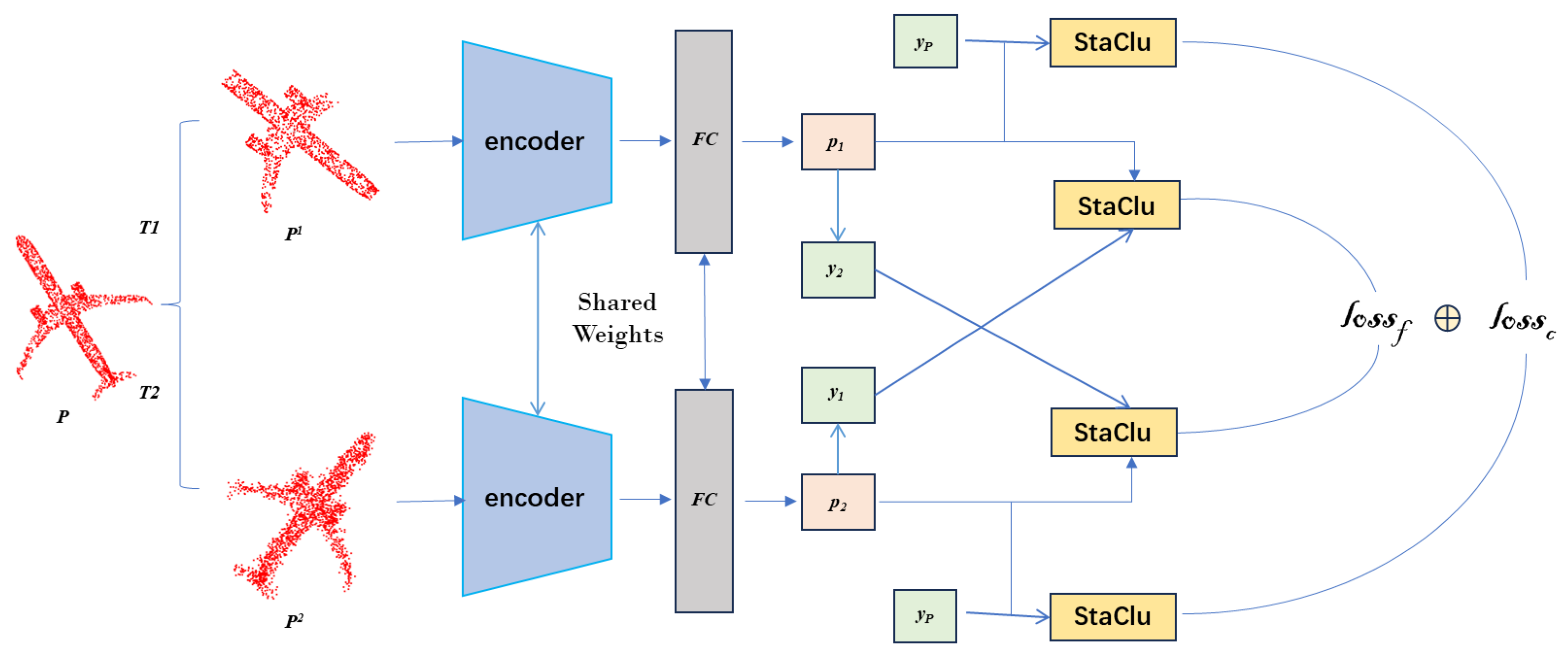
Given a dataset containing N point clouds , with the corresponding labels , the representations of these samples can be learned by optimizing a classification task. In order to mitigate the overfitting of the network, the traditional data enhancement was first performed on each data sample cluster to improve the diversity of the training samples while preserving the structure of the original data. Then, the universal DGCNN [5] was used as the backbone network to extract the features. The Dynamic Graph CNN (DGCNN) represents a sophisticated variant of graph convolutional networks, adept at dynamically apprehending and learning the intricate patterns within data structured as graphs. DGCNN achieves this through the synergy of graph convolution operations and the dynamic refinement of node attributes, proving efficacious for a spectrum of tasks including, but not limited to, node classification and graph matching. Besides the backbone network, a 2-layer MLP projection head is attached, and the output dimension is 128. After that, after the MLP header, the learned representation is classified by the fully connected (FC) layer encoding the clustering center, which has a size of 128 × K. At the same time, in the loss function, we adopted StaClu as the loss function module, which is embodied in stopping using the gradient of negative instances to update the cluster center in the cross entropy loss. Finally, as a clustering method, we set K to the number of real categories and used the direct predictions of the model as cluster assignments for evaluation. We evaluated our approach on ModelNet40 and the ShapeNet [39] benchmark dataset and achieved optimal results in the comparison methods. Figure 1 shows an overview of the framework process for our approach.
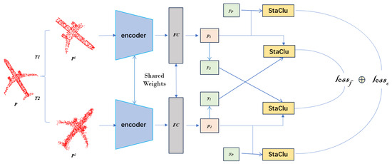
Figure 1.
PointStaClu’s framework process. In the figure, T represents point cloud data enhancement, and are enhanced views, and are predicted results after encoder input, is the label of a previous epoch, and are soft labels calculated by Equation (12), represents learning loss, and represents cluster center loss. The final loss is the sum of the two losses.
3.1. Cluster Discrimination
Given a dataset containing N point clouds , with the corresponding labels , the representations of these samples can be learned by optimizing a classification task.
where denotes the cross-entropy loss function with softmax normalization operation and θ represents the parameters of the deep neural network. For unsupervised learning with a lack of label information, the cluster discrimination objective on K clusters can be formulated as:
where represents the learnable label for the sample , and . The predicted value is computed as:
where , and indicates the encoder network. represents the network parameter of the encoder F. stands for the K clustering center. λ is the temperature parameter, after normalization .
In contrast to the supervised paradigm, the problem in Equation (2) must simultaneously optimize the cluster assignment , cluster center , and encoder network F.
3.2. Steady Loss for Small Batch Optimization
Unlike supervised learning, where instance labels are fixed, clustering in unsupervised learning is dynamic. The collocation changes dynamically as the instance representation and cluster center are trained. Consequently, the original cross-entropy loss, which relies on fixed instance labels, becomes unstable for unsupervised learning scenarios. This instability can be elucidated by analyzing the update criteria of the cluster center. Let represent the learnable label corresponding to , and let the gradient of of the standard cross-entropy loss in Equation (2) be calculated as:
The former is to pull the cluster center closer to the assigned instance, and the latter is to push it away from the other cluster instances. However, this update is unstable for deep clustering. The explanation is as follows:
- (a)
- When a small batch of b samples is taken for K clusters, at least K − b clusters have no positive instances at all. This means that in the case of cross-entropy loss, many clustering centers will only be updated by negative instances.
- (b)
- Let and represent the variance of the positive and negative instances of the sample, respectively. If each instance has a unit norm and the norm of the cluster mean is α, then there is . This shows that when each cluster is compact, i.e., α approaches 1, the variance of the negative instances sampled is much larger than the variance of the positive instances. Due to the small size of the small batches when training the deep neural networks, the variance cannot be sufficiently reduced.
Therefore, in many cases, the clustering center can only access a small batch of negative instances in each iteration, and the influence of negative instances is dominant. Unlike supervised learning with fixed labels, the cluster assignment of deep clustering changes continuously during training. Therefore, the update bias caused by the large variance in the negative instance will accumulate and mislead the learning process.
In order to alleviate this problem, we recommend the method of eliminating negative instance gradients for stability training:
The corresponding stable clustering discrimination loss (StaClu) is calculated as:
where indicates with a stop gradient operation. Compared with the standard cross entropy loss, the cluster center in the stable cluster discrimination loss is only updated by the positive instance, which is more stable for deep clustering using small batch optimization.
In k-means, positive instances have uniform weights when updating cluster centers:
where is the indicator function, and projects the vector to the unit norm. On the contrary, our proposed stable clustering discriminant objective implies novel difficult-sensing clustering criteria for deep clustering. When and are fixed, the for the loss function in Equation (6) is adopted for the problem of the optimal solution, and assuming ; 1, then we have:
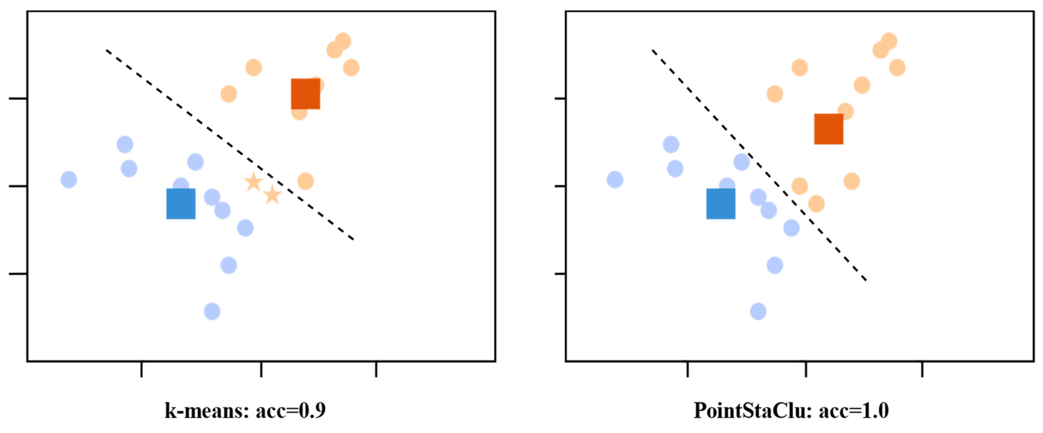
When updating the cluster center, our method assigns weights to instances based on their difficulty, i.e., . By assigning more weight to difficult instances ( smaller), the corresponding center can better capture the distribution of difficult instances, as shown in Figure 2.
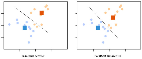
Figure 2.
Schematic diagram of difficulty sensing clustering criteria. Ten of the data points were randomly sampled from two different Gaussian distributions, with points of the same color coming from the same distribution, squares representing corresponding clustering centers obtained by different methods, and stars representing misclassified data.
In contrast to k-means, which apportions uniform weights across various instances, our methodology takes into account the intrinsic difficulty of each instance during the cluster center update process, rendering it more adept for discrimination-based clustering scenarios. Armed with the stable clustering discrimination (StaClu) loss function, we will provide an in-depth exposition of our proposed deep clustering method in the subsequent section.
3.3. Deep Clustering Based on Stable Clustering Discrimination
According to the proposed loss function, the stable clustering discrimination objective of deep clustering can be expressed by the following:
where , M represents the number of constraints, and is the first m clustering distribution constraint. Considering the interaction between the variables, we solve the problem alternately.
Update of . First, when fixing and of the previous epoch, the represented subproblem of learning of the t epoch is:
The stable cluster discrimination loss degenerates to standard cross-entropy loss, which can be optimized by the SGD optimizer. The one-hot tag is retained from the (t − 1) epoch, which makes the optimization consistent between adjacent epochs, but the update of the representation may be delayed. To consolidate the information about the current epoch, we include two enhanced views of a single instance in each iteration, which is popular in representation learning [40,41,42].
Let and be the two randomly enhanced views of the original point cloud, and the prediction is:
where the feature is extracted via the encoder in the current stage. The soft target for each enhanced view is calculated as follows, where is the weight for labels from the last epoch [43].
The soft target contains the predictions from another view of the same instance, which optimizes the consistency between the different views in the same iteration. The dual-view optimization problem is expressed as follows:
Update of . When fixing and , the assignment of the cluster can be updated by solving the following problem:
where is obtained via the calculation of and , as shown in Equation (3). Without constraint , the learning goal implies a greedy solution that assigns each instance to the most relevant cluster. It can lead to simple solutions that crash, especially for online deep clustering, where each instance can only be accessed once per epoch, and there is no way to perfect the cluster assignment with multiple iterations over the entire dataset.
Based on the above problems, we propose a global entropy constraint to balance the distribution of all the clusters. The boundary of the cluster size is implicit in the entropy constraint. Given the cluster allocation set , the entropy of the entire dataset is defined as:
Using entropy as regularization, the cluster assignment is updated by solving the following problems:
where γ is the ratio to the average size, and indicates the equilibrium constraint. The target controls the size of all the clusters simultaneously through only one constraint. According to the duality theory, this problem is equivalent to:
with dual view optimization, the update becomes:
Update of w. Fix and the pseudo-tag , and then optimize the clustering center by minimizing the stable clustering discrimination loss on the two enhanced views by using SGD:
The entire framework is illustrated in Algorithm 1:
| Algorithm 1 Pseudo-code of single-stage deep clustering based on stable clustering discrimination |
| Input: F: encoder network c: cluster center : cluster center from the last epoch y: list of pseudo one-hot labels : weight for labels from the last epoch λ: temperature |
| Initialization: keep the last cluster centers before each epoch. = c.detach() Train one epoch for P in loader do # load a minibatch with b samples = F(aug(P)), F(aug(P)) # two random enhanced views ) # retrieves the tag of the previous epoch Calculate the predictions for each view /λ) /λ) # soft labels are obtained for identification : loss of representational learning = (StaClu(, ) + StaClu (, ))/2 Update prediction is used for clustering .detach() @ c/λ) .detach() @ c/λ) Update cluster allocation using entropy constraints ) : loss of clustering center = (StaClu (, ) + StaClu (, ))/2 Update the encoder and clustering center loss.backward( ) end Output: Loss of stable discriminant clusters: loss |
4. Experiments and Results
To assess the efficacy of our method, we have undertaken an extensive series of experiments. This section delineates the performance metrics of PointStaClu within the domain of deep clustering, utilizing an established benchmark dataset, namely ModelNet40 and ShapeNet. ModelNet serves as a synthetic dataset designed for 3D object classification, whereas ShapeNet is an aggregation of CAD models sourced from an online, open-source repository, featuring 55 categories of synthetic 3D objects, including furniture, aircraft, vehicles, and humans.
4.1. Dataset and Evaluation Metrics
During the training phase, we adhered to the principle of a balanced dataset, ensuring a roughly equal number of samples per category, aligning with the configuration commonly employed in two-dimensional image clustering methods [17,44]. Additionally, we trained and evaluated our network on the complete dataset, eschewing the need to partition it into discrete training and test subsets. It should be noted that the test dataset was not constrained by the balanced assumption; we retained the option to conduct training and testing on a distinct dataset if desired. To forge a balanced dataset for conducting comprehensive clustering experiments, we amassed ten categories of point clouds, representing those with the most abundant samples, from the two preeminent benchmark datasets: ShapeNet and ModelNet40 [8]. The pertinent details regarding each of our balanced cloud datasets are encapsulated in Table 1. For each point cloud sample, we designated 2048 points as inputs, relying solely on the 3D coordinate data of these sampled points throughout our experiments.

Table 1.
Necessary details of the dataset.
Three standard clustering performance indexes were used to evaluate the performance of the clustering methods: Cluster Accuracy (ACC), Normalized Mutual Information (NMI) and Adjusted Rand Index (ARI) [45,46,47].
4.2. Implementation Details
In this section, we delineate the specific network architecture and training regimen of PointStaClu, aimed at attaining performance parity. Furthermore, we elucidate our optimization strategies and data augmentation methodologies, both of which are standard practices within the realm of unsupervised point cloud learning.
4.2.1. Architecture
To ensure a fair comparison with other methods, we adhered to standard practices for configuring the network architecture and training protocols. Specifically, we used the generic DGCNN as the backbone network to extract features. In addition to the backbone network, we added a 2-layer MLP projection head with 128 output dimensions. With the MLP header, the total number of parameters was almost the same as the original DGCNN. And after the MLP header, the learned representations were classified via the fully connected (FC) layer that encoded the clustering center. The size of the FC layer was 128 × K. As a clustering method, we set K to the number of real categories and used the model’s direct predictions as cluster assignments for evaluation. In addition, we used 10 different classification heads for clustering, which is conducive to target clustering. To avoid the problem of selecting suitable headers for evaluation when 10 headers had the same K, we used a different cK as the cluster number for each head, where , where the predicted result of the cluster head of c = 1 was used as the baseline for comparison.
4.2.2. Optimization
Before training the encoder network, we used an epoch to initialize the cluster allocation and center. The encoder network was optimized via SGD with a batch size of 48. Momentum and the learning rate were set at 0.9 and 0.05, respectively. Additionally, the first 10 epochs were used for warm-up, followed by Cosine annealing for the learning rate. For each dataset, the model was optimized with 300 epochs, and the cluster centers were learned with SGD at a constant learning rate of 0.3. The soft label parameter τ and temperature parameter in Equation (12) were fixed at 0.2 and 0.05, respectively. For the ModelNet40 dataset, the unique parameter α for the global entropy constraint was set to 700, and for the ShapeNet dataset, the parameter α was set to 2200. The parameter α was determined from the ablation studies on the corresponding dataset.
4.2.3. Enhancement
Data augmentation is pivotal to the efficacy of unsupervised representation learning. To ensure an equitable comparison, we implemented established settings utilized in prior works [11,40,41]. Specifically, we incorporated a suite of enhancement techniques, including random cropping, upsampling, flattening, rotation, scaling, jitter, and random discarding. The efficacy of these specific data enhancement methods was substantiated through the corresponding ablation study.
4.3. Comparative Experiment and Analysis of Clustering Performance
To demonstrate the superiority of our clustering algorithm relative to the existing methods, we performed comparative experiments on the two benchmark datasets, ShapeNet and ModelNet40. For the comparative analysis, we selected a range of algorithms, encompassing traditional clustering methods (K-Means++ [48], SC [49], AC [50]) as well as representation-based clustering approaches (STRL [40], PointMAE [25], PointM2AE [26], I2P-MAE [27]). Furthermore, to ensure a balanced comparison, we included DGCNN, which serves as the foundational network of our approach, as a representative of supervised learning methods. Table 2 presents the quantitative performance metrics of the compared methods, with those incorporating pre-training stages indicated as “multi-stage”.
Table 2.
Comparison of clustering methods on baseline dataset.
Through an exhaustive evaluation across the two distinct datasets, our method, PointStaClu, demonstrated a significant outperformance over the alternative methods across all the metrics. When juxtaposed with the traditional and representation-based clustering algorithms—typically employing K-means++ for post-processing—our end-to-end deep clustering framework excelled by optimizing the instance representations and delving into the data’s intrinsic distribution, rendering it exceptionally well-suited for clustering high-dimensional datasets, such as point clouds. Concurrently, PointStaClu, with its streamlined design featuring a solitary loss function and encoder and devoid of the need for supplementary pre-training, underscores the potency of our stable clustering discrimination task through its superior clustering performance. Furthermore, as depicted in the initial row of Table 2, PointStaClu’s clustering accuracy is marginally inferior to that of the supervised DGCNN method, exhibiting a negligible variance of 2.7% on the ShapeNet dataset (92.4% compared to 95.1%). On the ModelNet40 dataset, this disparity was even more reduced to 1.9% (96.6% compared to 98.5%), thereby substantially bridging the performance gap between unsupervised clustering and supervised classification within the point cloud domain.
4.4. Visual Experiment and Analysis
To provide an intuitive illustration of PointStaClu’s clustering capabilities, this section showcases the semantic clustering outcomes of our method alongside the representational features of point cloud samples obtained from a spectrum of clustering techniques, with PointStaClu being a key inclusion. These features were visualized through a t-SNE analysis conducted on the ShapeNet dataset.
4.4.1. Visualization of Semantic Clustering
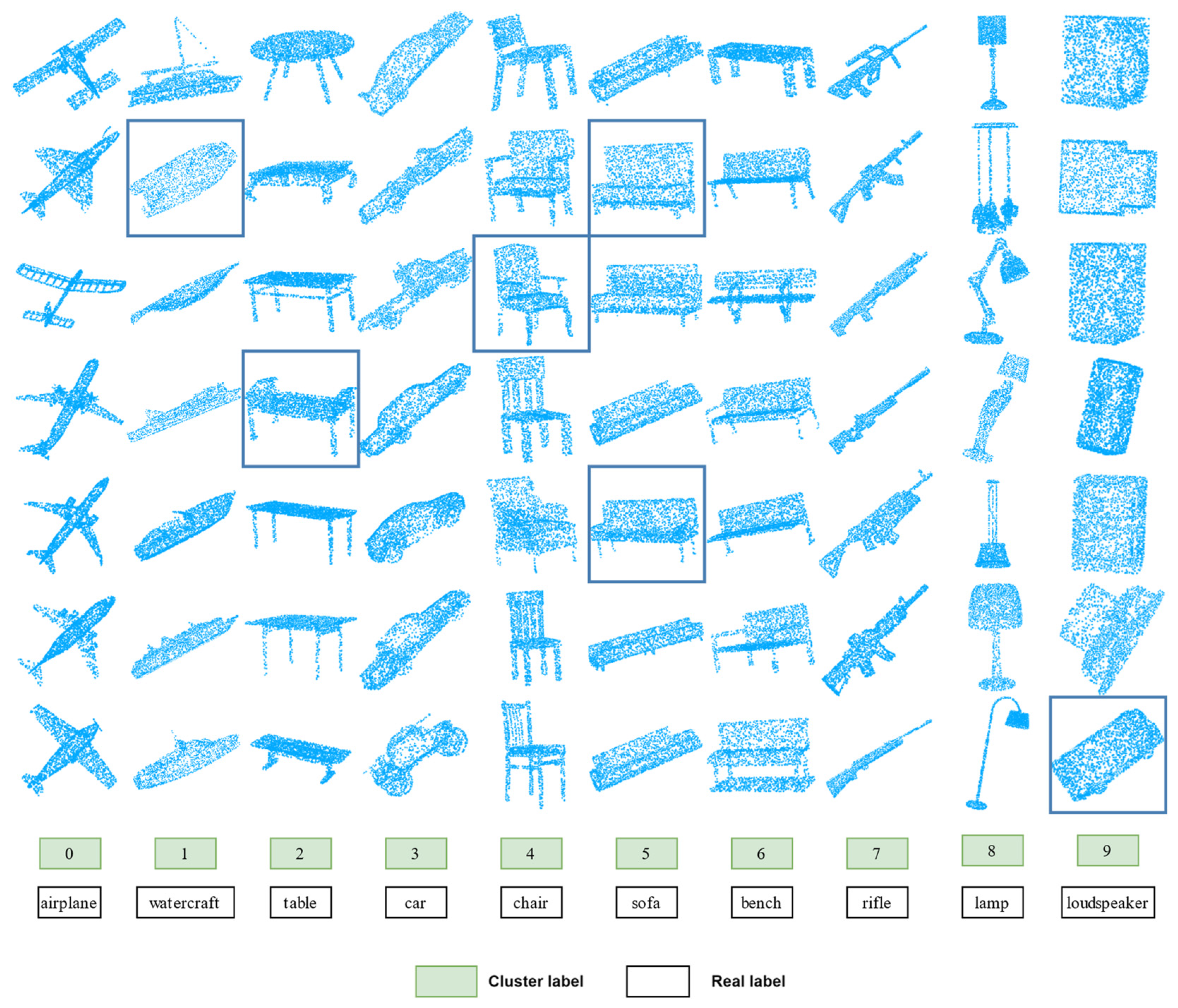
On the ShapeNet dataset, we present the semantic clustering outcomes as discerned by our method. For each cluster, a random selection of seven point cloud instances is displayed in Figure 3. The point clouds in each column are assigned to the same cluster. However, the samples with blue borders are misclassified and should actually belong to a different cluster. Specifically, the second point cloud in the second column should be classified as an aircraft, but it is incorrectly classified as a ship. Similarly, the last point cloud in the tenth column should be in the automotive category, not the audio category. In addition, confusion can easily arise between the categories of tables, sofas, and benches. In the table category, the fourth point cloud should be classified as a bench. And in the sofa category, there are two point clouds that should also be classified as benches. Overall, we observed that the cluster assignments obtained by our method mostly match natural clusters. The visual results show that our method successfully learns semantically meaningful clusters.
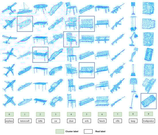
Figure 3.
Visualization of semantic clustering learned on ShapeNet.
4.4.2. Visualization of the Presentation Features
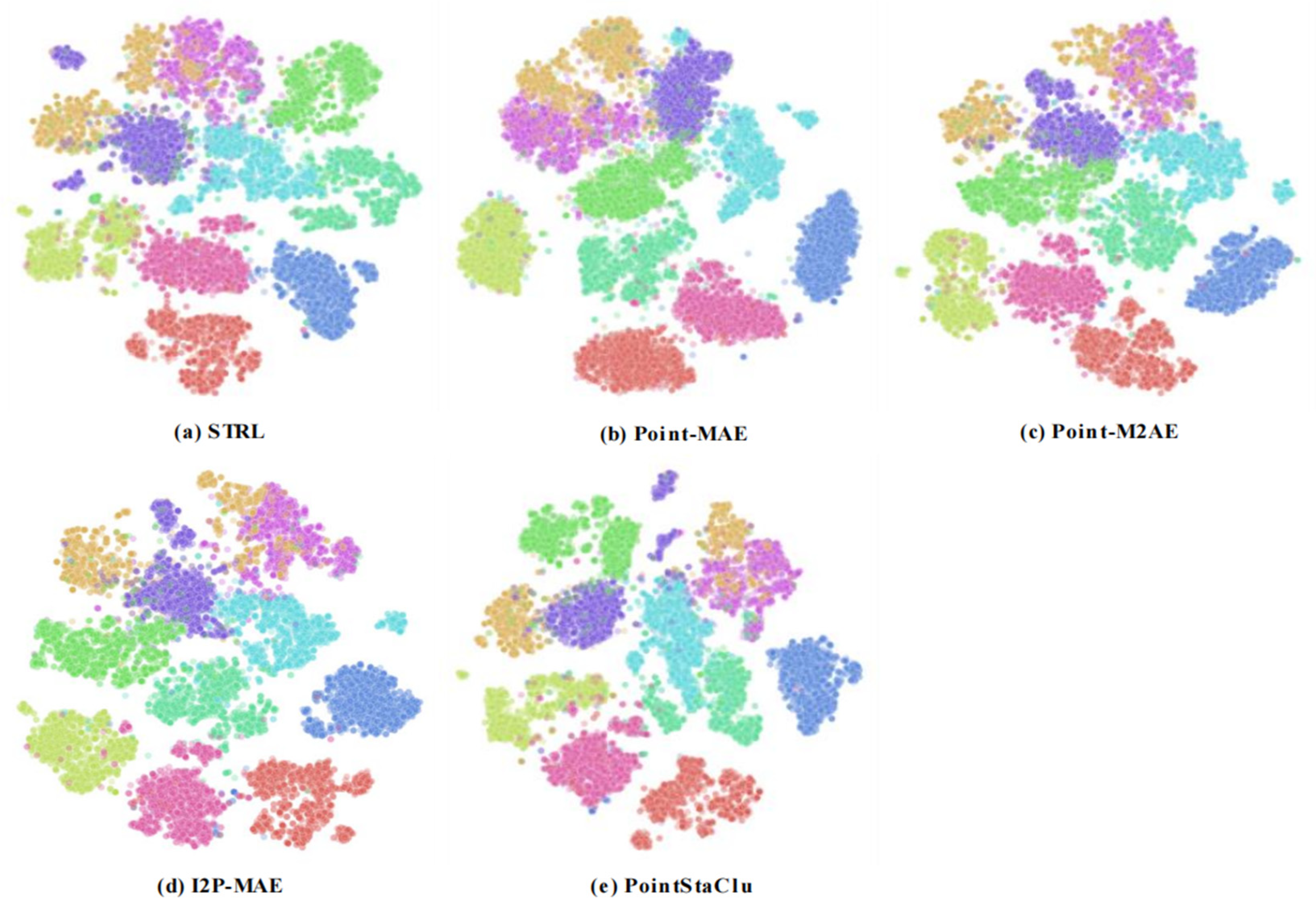
To ensure an equitable comparison, we utilized t-SNE for visualizing the representative features of the point cloud samples clustered via the methodologies enumerated in Table 2. As illustrated in Figure 4, the majority of the categories are discernible across all the evaluated methods, despite occasional imprecision or ill-defined boundaries in certain categories. In aggregate, the representative features gleaned by these clustering methodologies demonstrated no substantial disparities in quality. Notably, PointStaClu, our single-stage deep clustering approach, acquired the discernible features despite the absence of a distinct unsupervised representation learning phase, a fact corroborated by the visual outcomes. This highlights the efficacy of clustering as a viable precursor task in unsupervised learning. Consequently, PointStaClu is adept at mastering both instance representations and cluster allocations, thereby providing enhanced adaptability in data distribution modeling.
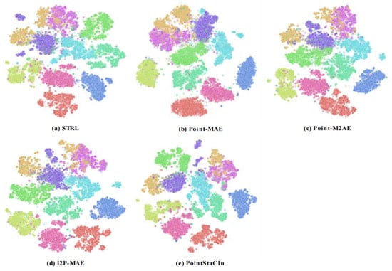
Figure 4.
Visualization of representation features learned by different clustering methods on ShapeNet dataset.
4.5. Sensitivity Analysis
To further elucidate and assess the significance of each component and setting within the proposed PointStaClu framework, we conducted comprehensive ablation studies on the ShapeNet dataset.
4.5.1. Effect of Negatives
Following the ablation experiments on our framework, we scrutinized the stable cluster discrimination loss, as articulated in Equation (6). We then juxtaposed its impact against the impact of the conventional standard cross-entropy loss (CE), as detailed in Table 3. The results clearly demonstrate that our method surpasses the cross-entropy-based approach when employing stable clustering, achieving a notable enhancement of approximately 37.1% in ACC, thereby affirming the essential role of our stable clustering discrimination loss. Moreover, upon examining the distribution of the learned clusters, it became apparent that, influenced by the global entropy constraint, the minimum cluster sizes across various loss functions exhibited negligible variation; in contrast, the maximum cluster sizes displayed considerable divergence. Utilizing our method to ascertain the stable clusters via the loss function, we observed a maximum cluster size of 1563 instances and a minimum of 1408 instances, closely mirroring the authentic distribution of the ShapeNet dataset, where each class encompasses 1489 instances. Conversely, the application of CE loss resulted in a maximum cluster size of 1989 instances and a minimum of 1326 instances, which significantly diverged from the dataset’s actual distribution. This divergence is attributable to the influence of negative instances, which impede the accurate learning of cluster centroids and consequently result in suboptimal cluster allocations.
Table 3.
The effect of loss function.
4.5.2. Effect of MLP Heads
In our PointStaClu clustering network architecture, as delineated in Table 4, a standard MLP layer for projection can be complemented with an additional prediction head MLP layer. We conducted a comparative analysis to assess the impact of varying the MLP header architectures on the performance of our method. In this context, “#Proj” and “#Pred” denote the MLP layers corresponding to the projection head and prediction head, respectively, with performance metrics including ACC (Cluster Accuracy), NMI (Normalized Mutual Information), and ARI (Adjusted Rand Index) presented in the table.
Table 4.
The effect of different numbers of MLP heads.
Initially, in the absence of both the projection and prediction head MLP layers, PointStaClu demonstrated a significant advantage over the other clustering methods in terms of accuracy (ACC), as documented in Table 4. This outcome confirms the efficacy of our deep clustering strategy. Introducing a single-layer MLP to the projection head further enhanced PointStaClu’s performance by 3.4%, suggesting that the integration of a dimensionality reduction layer is advantageous for the deep clustering process. Moreover, augmenting the projection head using a two-layer MLP configuration yielded an additional 2.3% improvement in ACC. However, the employment of more complex MLP layers in either the projection or prediction heads did not result in notable performance increments, indicating that a two-layer MLP is adequate for the point cloud dataset. Consequently, we elected to adopt the two-layer MLP for our projection head, eschewing the addition of further MLP layers in our final network architecture.
4.5.3. Effect of the α Parameter in Entropy Constraint
In our methodology, a global entropy constraint is employed to ensure an equitable cluster allocation. To ascertain the impact of the pivotal hyperparameter α within the entropy constraint on the clustering performance and distribution, we conducted experiments across a spectrum of α values, with the outcomes presented in Table 5.
Table 5.
The effect of α parameter in entropy constraint.
First, a larger α will make the distribution even, resulting in a suboptimal performance. By lowering the weights, the allocation becomes more flexible and the desired performance can be observed when α = 2200. However, a smaller α would result in an unbalanced distribution, which is not appropriate for our balanced dataset. α = 0 abandons the constraint and causes a crash. Obviously, entropy constraints can effectively balance the size of clusters, and using appropriate entropy constraints can not only obtain a relatively balanced cluster distribution but also obtain superior clustering results.
4.5.4. Effect of Data Enhancement Methods
Data enhancement is a key technique to enhance the performance of deep neural networks by increasing the number and diversity of training samples. Next, we will introduce the point cloud data enhancement method used in this method. Input the original point cloud as shown in Figure 5a, and the effect of each enhancement method is shown in Figure 5b–i, as follows:
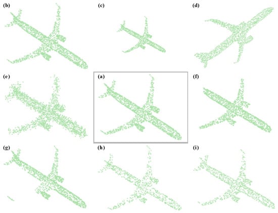
Figure 5.
Enhanced visualizations of point cloud data.
- (a)
- Translate, as shown in Figure 5b: for the input original point cloud, calculate its coordinate value range in the X, Y, and Z directions, and randomly move the whole point cloud object in each axial direction, and the moving distance is less than 10% of the original point cloud range;
- (b)
- Scale, as shown in Figure 5c: scale the entire point cloud sample to between 80% and 125% of the original point cloud;
- (c)
- Rotate, as shown in Figure 5d: the rotation method randomly rotates the point cloud object in three axial directions, X, Y, and Z, with a rotation range of 15 degrees;
- (d)
- Random jitter, as shown in Figure 5e: the three-dimensional position of each point is measured with a uniform random bias within the range of [0, 0.05];
- (e)
- Crop, as shown in Figure 5f: Sample evenly between 60% and 100% of the original 3D point cloud to crop out a random 3D cube patch. The aspect ratio is controlled within the range of [0.75, 1.33];
- (f)
- Cutout, as shown in Figure 5g: randomly cut out a three-dimensional cube, and each dimension of the three-dimensional cube is within the range of [0.1, 0.4] of the original dimension;
- (g)
- Drop out, as shown in Figure 5h: drop out three-dimensional points, and the ratio is within the range of [0, 0.7];
- (h)
- Subsampling, as shown in Figure 5i: randomly select some points from the three-dimensional point cloud, and the number of points is based on the input dimension of the encoder.
To investigate the impact of data augmentation on our method’s performance, we conducted comparative experiments using seven different augmentation techniques: random clipping, cutting, rotation, translation, scaling, jitter, and random discarding, with the results summarized in Table 6. Specifically, model used all the enhancement methods and achieved the best performance, in which the clustering accuracy (ACC) reached 92.4%. In contrast, model did not use any data enhancement, and the two views of the point cloud were identical. Therefore, the model cannot be driven to output consistent predictions for different transformations. The clustering performance was the worst, where the ACC dropped to 85.5%.
Table 6.
The effect of data enhancement methods.
Except for any of the enhancement methods, the clustering performance will decrease, which indicates that each enhancement method plays a positive role in the accurate clustering of point clouds. It is worth noting that when both clipping and clipping transformations were removed (model ), the network performance was significantly affected, and the ACC decreased by 5.1% (92.4% vs. 87.3%) compared with the full model . However, removing only the shear transform (model ) had the least effect on the network performance, because the shear transform broke the structural continuity of the point cloud to some extent, which is crucial for the point cloud representation learning. In addition, removing only the clipping transform (model ) resulted in a significant decline in clustering performance, suggesting that random clipping can significantly improve the performance.
4.5.5. Performance on an Imbalanced Dataset
In alignment with numerous 2D image clustering methodologies, our approach adheres to the principle of employing a balanced dataset for training purposes. Utilizing a balanced dataset promotes unbiased model training, averting the potential for class imbalances to distort the model’s focus. For the construction of a balanced dataset to conduct extensive clustering experiments, we selected the widely recognized ShapeNet benchmark. From this dataset, which includes a diverse range of point clouds, we curated ten categories that represented the highest number of point cloud samples (imbalance level ζ = 1) [51]. Table 7 illustrates the results derived from training our model on both the balanced and imbalanced datasets, characterized by the imbalance levels ζ = 0.8 and 0.6, within the aforementioned benchmark dataset.
Table 7.
Performance on an imbalanced dataset (imbalance level ζ).
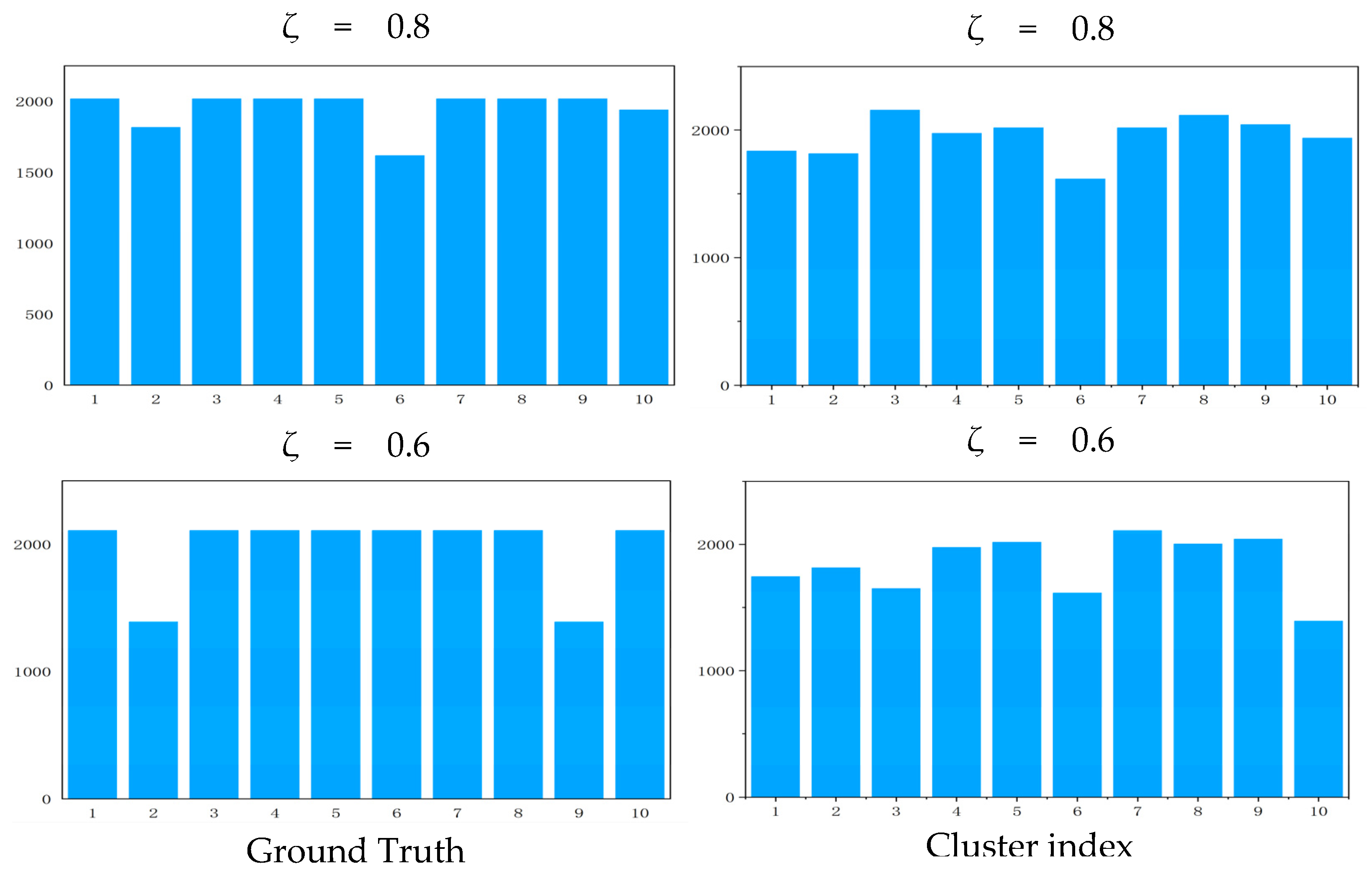
The objective of this evaluation was to assess the robustness of our approach when applied to an imbalanced dataset. As depicted in Table 7, we generated three levels of imbalanced dataset with ζ = 1.0, 0.8, 0.6, respectively, where 1.0 means a balanced dataset and the smaller the ζ, the more the imbalance. The distribution of clusters presented in Figure 6 provides a visual complement to the numerical findings. However, a reduction in the level of imbalance corresponds to a decrement in clustering performance, suggesting that the performance of our method on an imbalanced dataset requires further enhancement.
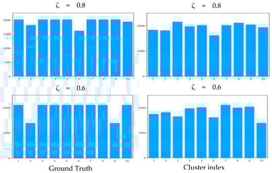
Figure 6.
Cluster distribution on imbalanced dataset. The first column is the cluster distribution of the original dataset, and the second column is the cluster distribution under the imbalance level ζ = 0.8 and 0.6. The horizontal axis of each statistical graph is cluster index and the vertical axis is samples.
5. Discussion
Our proposed PointStaClu method marks a significant advancement in the realm of point cloud clustering, effectively bridging the performance gap between unsupervised clustering and supervised classification within the domain of 3D point clouds. PointStaClu addresses the training instability inherent in supervised learning for 3D point cloud clustering through the following strategies: (1) The exclusion of negative instance gradients in the cross-entropy loss function updates for cluster centers; (2) The incorporation of a global entropy constraint to enhance the cluster allocation; and (3) The provision of a streamlined framework that employs a single loss function and encoder for deep point cloud clustering. Our approach, rigorously validated through extensive benchmark testing, exemplifies the robust clustering capabilities and exhibits an enhancement in performance for single-stage deep point cloud clustering.
While PointStaClu boasts an impressive performance, it is not without limitations. The method presupposes prior knowledge of the cluster category K, information that may be inscrutable in real-world datasets, thereby complicating the network training process. Furthermore, PointStaClu necessitates a balanced sample distribution, a condition that is not consistently observed in real-world data. Future research, focusing on imbalanced datasets and the potential integration of the nearest neighbor techniques, could further enhance the efficacy of PointStaClu.
6. Conclusions
In summary, PointStaClu pioneers the integration of a stable clustering discriminant task alongside an entropy constraint strategy, both aimed at refining the clustering allocation in an unsupervised manner. Its superior performance over the existing methodologies substantiates the efficacy of single-stage deep clustering for point clouds. Considering the dearth of research on single-stage deep clustering within the 3D point cloud domain, PointStaClu significantly advances the collective comprehension and application potential of point cloud learning endeavors.
Author Contributions
Conceptualization, X.C. and H.W.; methodology, X.C. and X.L.; software, X.C.; validation, X.C. and Y.W.; formal analysis, X.C.; investigation, X.C.; resources, Q.Z.; data curation, K.L.; writing—original draft preparation, X.C.; writing—review and editing, L.S.; supervision, L.S.; project administration, L.S.; funding acquisition, L.S. All authors have read and agreed to the published version of the manuscript.
Funding
This research was funded in part by the Key Research and Development Program of Shaanxi Province (2024SF-YBXM-681, 2019GY215, 2021ZDLSF06-04) and in part by the National Natural Science Foundation of China (61701403,61806164).
Data Availability Statement
The data presented in this study are openly available in Reference [31].
Conflicts of Interest
The authors declare no conflicts of interest.
References
- Xu, Y.; Arai, S.; Liu, D.; Lin, F.; Kosuge, K. FPCC: Fast point cloud clustering-based instance segmentation for industrial bin-picking. Neurocomputing 2022, 494, 255–268. [Google Scholar] [CrossRef]
- Ye, N.; Zhu, H.; Wei, M.; Zhang, L. Accurate and dense point cloud generation for industrial Measurement via target-free photogrammetry. Opt. Lasers Eng. 2021, 140, 106521. [Google Scholar] [CrossRef]
- Yin, C.; Wang, B.; Gan, V.J.; Wang, M.; Cheng, J.C. Automated semantic segmentation of industrial point clouds using ResPointNet++. Autom. Constr. 2021, 130, 103874. [Google Scholar] [CrossRef]
- Li, Y.; Bu, R.; Sun, M.; Wu, W.; Di, X.; Chen, B. Pointcnn: Convolution on x-transformed points. Adv. Neural Inf. Process. Syst. 2018, 31, 828–838. [Google Scholar]
- Wang, Y.; Sun, Y.; Liu, Z.; Sarma, S.E.; Bronstein, M.M.; Solomon, J.M. Dynamic graph cnn for learning on point clouds. ACM Trans. Graph. 2019, 38, 146. [Google Scholar] [CrossRef]
- Ran, H.; Zhuo, W.; Liu, J.; Lu, L. Learning inner-group relations on point clouds. In Proceedings of the IEEE/CVF International Conference on Computer Vision, Montreal, BC, Canada, 11–17 October 2021; pp. 15477–15487. [Google Scholar]
- Qi, C.R.; Su, H.; Mo, K.; Guibas, L.J. Pointnet: Deep learning on point sets for 3d classification and segmentation. In Proceedings of the IEEE Conference on Computer Vision and Pattern Recognition, Honolulu, HI, USA, 21–26 July 2017; pp. 652–660. [Google Scholar]
- Wu, Z.; Song, S.; Khosla, A.; Yu, F.; Zhang, L.; Tang, X.; Xiao, J. 3d shapenets: A deep representation for volumetric shapes. In Proceedings of the IEEE Conference on Computer Vision and Pattern Recognition, Santiago, Chile, 7–13 December 2015; pp. 1912–1920. [Google Scholar]
- Ma, X.; Qin, C.; You, H.; Ran, H.; Fu, Y. Rethinking network design and local geometry in point cloud: A simple residual MLP framework. arXiv 2022, arXiv:2202.07123. [Google Scholar]
- Uy, M.A.; Pham, Q.-H.; Hua, B.-S.; Nguyen, T.; Yeung, S.-K. Revisiting point cloud classification: A new benchmark dataset and classification model on real-world data. In Proceedings of the IEEE/CVF International Conference on Computer Vision, Seoul, Republic of Korea, 27 October–2 November 2019; pp. 1588–1597. [Google Scholar]
- Rao, Y.; Lu, J.; Zhou, J. PointGLR: Unsupervised structural representation learning of 3D point clouds. IEEE Trans. Pattern Anal. Mach. Intell. 2022, 45, 2193–2207. [Google Scholar] [CrossRef] [PubMed]
- Xiang, T.; Zhang, C.; Song, Y.; Yu, J.; Cai, W. Walk in the cloud: Learning curves for point clouds shape analysis. In Proceedings of the IEEE/CVF International Conference on Computer Vision, Montreal, BC, Canada, 11–17 October 2021; pp. 915–924. [Google Scholar]
- Zhao, H.; Jiang, L.; Jia, J.; Torr, P.H.; Koltun, V. Point transformer. In Proceedings of the IEEE/CVF International Conference on Computer Vision, Montreal, BC, Canada, 11–17 October 2021; pp. 16259–16268. [Google Scholar]
- Wu, Z.; Xiong, Y.; Yu, S.X.; Lin, D. Unsupervised feature learning via non-parametric instance discrimination. In Proceedings of the IEEE Conference on Computer Vision and Pattern Recognition, Salt Lake City, UT, USA, 18–23 June 2018; pp. 3733–3742. [Google Scholar]
- MacQueen, J. Some Methods for Classification and Analysis of Multivariate Observations. In Proceedings of the Fifth Berkeley Symposium on Mathematical Statistics and Probability, Berkeley, CA, USA, 21 June–18 July 1965, 27 December 1965–7 January 1966; University of California Press: Berkeley, CA, USA, 1967; pp. 281–297. Available online: https://books.google.com.sg/books?hl=zh-CN&lr=&id=IC4Ku_7dBFUC&oi=fnd&pg=PA281&ots=nQTkKVMbtN&sig=s5CdqqD5NRDI_Hz0qDdsPWYglqk&redir_esc=y#v=onepage&q&f=false (accessed on 12 May 2024).
- Caron, M.; Bojanowski, P.; Joulin, A.; Douze, M. Deep clustering for unsupervised learning of visual features. In Proceedings of the European Conference on Computer Vision (ECCV), Munich, Germany, 8–14 September 2018; pp. 132–149. [Google Scholar]
- Li, Y.; Yang, M.; Peng, D.; Li, T.; Huang, J.; Peng, X. Twin contrastive learning for online clustering. Int. J. Comput. Vis. 2022, 130, 2205–2221. [Google Scholar] [CrossRef]
- Huang, J.; Gong, S.; Zhu, X. Deep semantic clustering by partition confidence maximisation. In Proceedings of the IEEE/CVF Conference on Computer Vision and Pattern Recognition, Seattle, WA, USA, 13–19 June 2020; pp. 8849–8858. [Google Scholar]
- Van Gansbeke, W.; Vandenhende, S.; Georgoulis, S.; Proesmans, M.; Van Gool, L. Scan: Learning to classify images without labels. In Proceedings of the European Conference on Computer Vision, Glasgow, UK, 23–28 August 2020; pp. 268–285. [Google Scholar]
- Yang, Y.; Feng, C.; Shen, Y.; Tian, D. Foldingnet: Point cloud auto-encoder via deep grid deformation. In Proceedings of the IEEE Conference on Computer Vision and Pattern Recognition, Salt Lake City, UT, USA, 18–23 June 2018; pp. 206–215. [Google Scholar]
- Wu, J.; Zhang, C.; Xue, T.; Freeman, B.; Tenenbaum, J. Learning a probabilistic latent space of object shapes via 3d generative-adversarial modeling. Adv. Neural Inf. Process. Syst. 2016, 29, 82. [Google Scholar]
- Li, C.-L.; Zaheer, M.; Zhang, Y.; Poczos, B.; Salakhutdinov, R. Point cloud gan. arXiv 2018, arXiv:1810.05795. [Google Scholar]
- Xiao, A.; Huang, J.; Guan, D.; Zhang, X.; Lu, S.; Shao, L. Unsupervised point cloud representation learning with deep neural networks: A survey. IEEE Trans. Pattern Anal. Mach. Intell. 2023, 45, 11321–11339. [Google Scholar] [CrossRef] [PubMed]
- Xie, S.; Gu, J.; Guo, D.; Qi, C.R.; Guibas, L.; Litany, O. Pointcontrast: Unsupervised Pre-training for 3d Point Cloud Understanding. In Proceedings of the Computer Vision—ECCV 2020: 16th European Conference, Glasgow, UK, 23–28 August 2020; Proceedings, Part III 16. pp. 574–591. [Google Scholar]
- Pang, Y.; Wang, W.; Tay, F.E.; Liu, W.; Tian, Y.; Yuan, L. Masked autoencoders for point cloud self-supervised learning. In Proceedings of the European Conference on Computer Vision, Tel Aviv, Israel, 23–27 October 2022; pp. 604–621. [Google Scholar]
- Zhang, R.; Guo, Z.; Gao, P.; Fang, R.; Zhao, B.; Wang, D.; Qiao, Y.; Li, H. Point-m2ae: Multi-scale masked autoencoders for hierarchical point cloud pre-training. Adv. Neural Inf. Process. Syst. 2022, 35, 27061–27074. [Google Scholar]
- Zhang, R.; Wang, L.; Qiao, Y.; Gao, P.; Li, H. Learning 3d representations from 2d pre-trained models via image-to-point masked autoencoders. In Proceedings of the IEEE/CVF Conference on Computer Vision and Pattern Recognition, Vancouver, BC, Canada, 17–24 June 2023; pp. 21769–21780. [Google Scholar]
- Caron, M.; Misra, I.; Mairal, J.; Goyal, P.; Bojanowski, P.; Joulin, A. Unsupervised learning of visual features by contrasting cluster assignments. Adv. Neural Inf. Process. Syst. 2020, 33, 9912–9924. [Google Scholar]
- Qian, Q. Stable cluster discrimination for deep clustering. In Proceedings of the IEEE/CVF International Conference on Computer Vision, Vancouver, BC, Canada, 17–24 June 2023; pp. 16645–16654. [Google Scholar]
- Zhang, L.; Zhu, Z. Unsupervised feature learning for point cloud understanding by contrasting and clustering using graph convolutional neural networks. In Proceedings of the 2019 International Conference on 3D Vision (3DV), Quebec City, QC, Canada, 16–19 September 2019; pp. 395–404. [Google Scholar]
- Hassani, K.; Haley, M. Unsupervised multi-task feature learning on point clouds. In Proceedings of the IEEE/CVF International Conference on Computer Vision, Seoul, Republic of Korea, 27 October–2 November 2019; pp. 8160–8171. [Google Scholar]
- Li, J.; Chen, B.M.; Lee, G.H. So-net: Self-organizing network for point cloud analysis. In Proceedings of the IEEE Conference on Computer Vision and Pattern Recognition, Salt Lake City, UT, USA, 18–23 June 2018; pp. 9397–9406. [Google Scholar]
- Girdhar, R.; Fouhey, D.F.; Rodriguez, M.; Gupta, A. Learning a predictable and generative vector representation for objects. In Proceedings of the Computer Vision—ECCV 2016: 14th European Conference, Amsterdam, The Netherlands, 11–14 October 2016; Proceedings, Part VI 14. pp. 484–499. [Google Scholar]
- Achlioptas, P.; Diamanti, O.; Mitliagkas, I.; Guibas, L. Learning representations and generative models for 3d point clouds. In Proceedings of the International Conference on Machine Learning, Vienna, Austria, 10–15 July 2018; pp. 40–49. [Google Scholar]
- Liu, F.; Lin, G.; Foo, C.-S. Point discriminative learning for unsupervised representation learning on 3D point clouds. arXiv 2021, arXiv:2108.02104. [Google Scholar]
- Asano, Y.M.; Rupprecht, C.; Vedaldi, A. Self-labelling via simultaneous clustering and representation learning. arXiv 2019, arXiv:1911.05371. [Google Scholar]
- Chen, T.; Kornblith, S.; Norouzi, M.; Hinton, G. A simple framework for contrastive learning of visual representations. In Proceedings of the International Conference on Machine Learning, Online, 13–18 July 2020; pp. 1597–1607. [Google Scholar]
- Dang, Z.; Deng, C.; Yang, X.; Wei, K.; Huang, H. Nearest neighbor matching for deep clustering. In Proceedings of the IEEE/CVF Conference on Computer Vision and Pattern Recognition, Nashville, TN, USA, 20–25 June 2021; pp. 13693–13702. [Google Scholar]
- Chang, A.X.; Funkhouser, T.; Guibas, L.; Hanrahan, P.; Huang, Q.; Li, Z.; Savarese, S.; Savva, M.; Song, S.; Su, H. Shapenet: An information-rich 3d model repository. arXiv 2015, arXiv:1512.03012. [Google Scholar]
- Huang, S.; Xie, Y.; Zhu, S.-C.; Zhu, Y. Spatio-temporal self-supervised representation learning for 3d point clouds. In Proceedings of the IEEE/CVF International Conference on Computer Vision, Montreal, BC, Canada, 11–17 October 2021; pp. 6535–6545. [Google Scholar]
- Afham, M.; Dissanayake, I.; Dissanayake, D.; Dharmasiri, A.; Thilakarathna, K.; Rodrigo, R. Crosspoint: Self-supervised cross-modal contrastive learning for 3d point cloud understanding. In Proceedings of the IEEE/CVF Conference on Computer Vision and Pattern Recognition, New Orleans, LA, USA, 18–24 June 2022; pp. 9902–9912. [Google Scholar]
- Wu, Y.; Liu, J.; Gong, M.; Gong, P.; Fan, X.; Qin, A.; Miao, Q.; Ma, W. Self-supervised intra-modal and cross-modal contrastive learning for point cloud understanding. IEEE Trans. Multimed. 2023, 26, 1626–1638. [Google Scholar] [CrossRef]
- Qian, Q.; Xu, Y.; Hu, J.; Li, H.; Jin, R. Unsupervised visual representation learning by online constrained k-means. In Proceedings of the IEEE/CVF Conference on Computer Vision and Pattern Recognition, New Orleans, LA, USA, 18–24 June 2022; pp. 16640–16649. [Google Scholar]
- Huang, Z.; Chen, J.; Zhang, J.; Shan, H. Learning representation for clustering via prototype scattering and positive sampling. IEEE Trans. Pattern Anal. Mach. Intell. 2022, 45, 7509–7524. [Google Scholar] [CrossRef] [PubMed]
- Zhou, S.; Xu, H.; Zheng, Z.; Chen, J.; Bu, J.; Wu, J.; Wang, X.; Zhu, W.; Ester, M. A comprehensive survey on deep clustering: Taxonomy, challenges, and future directions. arXiv 2022, arXiv:2206.07579. [Google Scholar]
- Min, E.; Guo, X.; Liu, Q.; Zhang, G.; Cui, J.; Long, J. A survey of clustering with deep learning: From the perspective of network architecture. IEEE Access 2018, 6, 39501–39514. [Google Scholar] [CrossRef]
- Kuhn, H.W. The Hungarian method for the assignment problem. Nav. Res. Logist. Q. 1955, 2, 83–97. [Google Scholar] [CrossRef]
- Arthur, D.; Vassilvitskii, S. K-means++: The Advantages of Careful Seeding; Stanford University: Stanford, CA, USA, 2007; pp. 1027–1035. [Google Scholar]
- Ng, A.; Jordan, M.; Weiss, Y. On spectral clustering: Analysis and an algorithm. Adv. Neural Inf. Process. Syst. 2001, 14, 849–856. [Google Scholar]
- Franti, P.; Virmajoki, O.; Hautamaki, V. Fast agglomerative clustering using a k-nearest neighbor graph. IEEE Trans. Pattern Anal. Mach. Intell. 2006, 28, 1875–1881. [Google Scholar] [CrossRef]
- Niu, C.; Shan, H.; Wang, G. Spice: Semantic pseudo-labeling for image clustering. IEEE Trans. Image Process. 2022, 31, 7264–7278. [Google Scholar] [CrossRef] [PubMed]

Disclaimer/Publisher’s Note: The statements, opinions and data contained in all publications are solely those of the individual author(s) and contributor(s) and not of MDPI and/or the editor(s). MDPI and/or the editor(s) disclaim responsibility for any injury to people or property resulting from any ideas, methods, instructions or products referred to in the content. |
© 2024 by the authors. Licensee MDPI, Basel, Switzerland. This article is an open access article distributed under the terms and conditions of the Creative Commons Attribution (CC BY) license (https://creativecommons.org/licenses/by/4.0/).