
Monitoring Water Diversity and Water Quality with Remote Sensing and Traits
 , , , , , , , , , , and
Abstract
:1. Introduction
2. Definition and Standards of Water Quality and Water Characteristics
Standards and Guidelines
3. Definition of Water Diversity Using Remote Sensing
- (I)
- The diversity of water traits, which represents the diversity of the biochemical-, physical, optical, morphological-, structural-, textural- and functional characteristics of water traits that affect, interact with or are influenced by their genesis-, taxonomic-, structural- and functional diversity;
- (II)
- The diversity of water genesis, which refers to the diversity of the length of evolutionary pathways associated with a particular set of water traits, taxa, structures and functions of water diversity. Therefore, groups of water traits, water taxa, water structures and water functions that maximise the accumulation of functional diversity of water diversity are identified;
- (II)
- The structural diversity of water, namely, the diversity of the composition and configuration of water characteristics;
- (IV)
- The taxonomic diversity of water, representing the diversity of water components that differ from a taxonomic perspective;
- (V)
- The functional diversity of water, which is the diversity of water functions and processes, as well as their intra- and interspecific interactions.
4. Approaches for Monitoring Water Diversity and Water Quality
4.1. In Situ Approaches
4.2. Remote Sensing Approach
- The spatial and temporal resolution of RS data: many bodies of water change rapidly both spatially and temporally. Sensors with insufficient spatial or temporal resolution may therefore not be able to provide accurate or up-to-date data.
- The heterogeneity of water bodies: water bodies are often heterogeneous in their composition. Different areas of a water body can have different characteristics, which complicates the analysis and interpretation of RS data.
- The spectral signature of substances: various substances in water (such as chlorophyll, dissolved organic matter and sediments) have specific spectral signatures. The precise identification and quantification of these substances require specialised sensors and complex analysis methods.
- Technical limitations: the available technology, in particular the spectral and spatial resolution of the sensors, as well as the limited availability of validation data sets, limits what can be recorded and analysed.
- Interdisciplinary challenges: the correct interpretation of RS data with regard to water quality often requires a deep understanding of different scientific disciplines, including limnology, oceanography and environmental sciences.
4.2.1. Monitoring the Diversity of Water Traits Using Remote Sensing
4.2.2. Monitoring the Diversity of Water Genese Using Remote Sensing
4.2.3. Monitoring the Structural Diversity of Water Using Remote Sensing
4.2.4. Monitoring the Taxonomic Diversity of Water with Remote Sensing
4.2.5. Monitoring the Functional Diversity of Water with Remote Sensing
5. Conclusions and Further Research
Author Contributions
Funding
Data Availability Statement
Acknowledgments
Conflicts of Interest
Appendix A


| Water Traits | Mission/Platform Sensor | References |
|---|---|---|
| Sea surface temperature (SST), river surface temperature (RST) | GOES-8 IMAGER 3, METEOSAT (MSG) SEVIRI 3, NOAA POES AVHRR 3, Aqua MODIS 3, Terra ASTER 3, Landsat 5 TM 3, Landsat 7 ETM+ 3, ERS-1/-2/ATSR1 3, FLIR Tau 2 | [197,198,199,200,201,202,203,204,205,206,207,208,209,210,211] |
| Chlorophyll-a (CHL)—phytoplankton (large/small phytoplankton) | OrbView-2 SeaWiFS 3, Terra/Aqua MODIS 3, Envisat MERIS 3, Sentinel-3 OLCI 3, Sentinel-2 3, Landsat 8 OLI/TIRS 3, APEX 2, LiDAR 1 | [23,186,212,213,214,215,216,217,218,219,220,221,222,223,224,225,226,227,228,229,230,231] |
| Phycocyanin (PC) and phycoerythrin—other photosynthetic and accessory pigments (cyanobacterial blooms indicated by phycocyanin (PC) and phycoerythrin) | Terra/Aqua MODIS 3, Sentinel-3 OLCI 3, Landsat 8 OLI/TIRS 3, NOAA GLERL 2, Sentinel-2 MSI 3 | [214,219,220,221,232,233] |
| Fluorescence—sun-induced fluorescence emission by phytoplankton/open-ocean phytoplankton chlorophyll fluorescence, (Fsat) distributions | Terra/Aqua MODIS 3 | [219,229,234] |
| Chemical oxygen demand concentration (CCOD) Water pollution | Sentinel 3 A/Ocean 3, Land Colour Instrument (OLCI) 3 | [235] |
| Algal blooms indicator (HAB)/Cyanobacterial Harmful Algal Bloom(s) (CHAB) | Landsat 8 3, Sentinel-2A,2B 3, Sentinel-3A, 3B, 3C 3, WorldView-3 3, PRISMA 3 | [236,237,238,239] |
| Phytoplankton populations, community structures (e.g., phaeocystis and diatoms, phaeocystis globosa spp) | OrbView-2 SeaWiFS 3 | [219,240] |
| Aquatic Phytoplankton Functional Types (A-PFTs) | OrbView-2 SeaWiFS 3, MERIS 3, APEX 2 | [188,219,241,242] |
| Macrobenthos, macrophytes—submerged aquatic vegetation (SAV) | QuickBird BGIS2000 3, RapidEye REIS 3, Sentinel-2 3, Landsat 8 OLI/TIRS 3, HJ-WVC 3, Daedalus MIVIS 2, Ocean Portable Hyperspectral Imager for Low-Light 2, Spectroscopy (Ocean PHILLS) 2, VarioCAM 1 | [82,228,243,244,245,246,247,248,249,250] |
| Lake-type classification | Landsat TM/ETM +/OLI 3, ASTER GDEM 3 | [78,251] |
| Optical water types (OWTs) | Sentinel-3 OLCI 3 | [214] |
| Channel landforms, hydrogeomorphic units including coarse woody debris, hydraulic (fluvial) landform classification, hydro-morphological units, riverscape units, river geomorphic units, in-stream mesohabitats, tidal channel characteristics | SAR 3, aerial images 2, LiDAR 2 | [252,253,254,255] |
| Coast taxonomy, coast types (small delta, tidal system, lagoon, fjord and fjärd, large river, tidal estuary, ria, karst, arheic) | Different RADAR sensors 3, different optical RS sensors 3 | [179] |
| Macrophyte taxonomy/macrophyte taxa/aquatic plant species | Canon Ixus 70 ® 1, Sentinel 2 3 Airborne Hyperspectral 2 | [167,256] |
| Coral classification, coral reef habitat mapping, seagrass, aquatic vegetation community | Landsat 8 OLI/TIRS 3, RapidEye REIS 3, Ocean Portable Hyperspectral Imager for Low-Light 3, Spectroscopy (Ocean PHILLS) 2, Sentinel-2 3, QuickBird 3, WorldView 3, NOAA 3 Worldview-2 3, HyMAP 2, airborne (imaging spectrometer (hyperspectral) 2, Planet Dove satellite imagery 2, Airborne data visible-to-shortwave infrared 2, (VSWIR) imaging spectrometer and a light detection and ranging 2 LiDAR 2, CASI 2 | [113,151,219,249,257,258,259,260,261,262,263] |
| Coral mortality | Airborne data visible-to-shortwave infrared 2, (VSWIR) imaging spectrometer and a light detection and ranging 2, LiDAR 2 | [261] |
| Live coral cover density | Airborne data visible-to-shortwave infrared 2, VSWIR imaging spectrometer and a light detection and ranging 2, LiDAR 2 | [151] |
| Reef rugosity | LiDAR 2, VSWIR spectrometer Data 2 | [264] |
| Macrophyte canopy morphological traits (MTs)—fractional cover (fc) | APEX 2 | [242] |
| Macrophyte—Leaf Area Index (LAI) | Spot-5 HRG 3, Sentinel-2 MSI 3 Landsat 7 ETM+ 3, Landsat 8 OLI/TIRS 3, APEX 2 | [242,245] |
| Above-water biomass | Landsat 8 OLI/TIRS 3, Terra/Aqua MODIS 3, Landsat 8 OLI/TIRS 3, GaoFen-1 WFV 3, WorlsView-2 WV110 3, APEX 2 | [242,265,266] |
| Macrophyte seasonal dynamics (phenology)/spatial distribution patterns/species-dependent variability, interannual changes of aquatic vegetation | Spot-5 HRG 3, Sentinel-2 MSI 3, Landsat 7 ETM+ 3, Landsat 8 OLI/TIRS 3, HJ-1A/B WVC 3, Landsat 5 TM 3 | [245,267] |
| Growth height of submerged aquatic vegetation (SAV) | Spot-6 NAOMI 3 | [268] |
| Suspended Particulate Matter (SPM), also referred to as the Total Suspended Matter (TSM) | Envisat MERIS 3, Terra/Aqua MODIS 3, Landsat 8 OLI/TIRS 3, Sentinel 3 OLCI 3, AHS 2 | [23,219,224,265,269,270,271,272] |
| Suspended Sediment Concentration (SSC) | Envisat MERIS 3 | [219,273] |
| Suspended inorganic particulate matter (SPIM) | Sentinel-2 MSI 3, Daedalus MIVIS 2 | [219,248,274] |
| Coloured Dissolved Organic Matter (CDOM) | OrbView-2 SeaWiFS 3, Envisat MERIS 3, Landsat 5 TM 3 < Landsat 7 ETM+ 3, Landsat 8 OLI/TIRS 3, Sentinel-2 MSI 3,Sentinel-3 OLCI 3, Daedalus MIVIS 2 | [23,212,217,219,222,224,248,275,276] |
| Sediment and sediment dynamic, carbon and nutrient loads, particulate organic carbon (POC) | EO-1 Hyperion 3, Terra/Aqua MODIS 3, Landsat 5 TM 3, Landsat 7 ETM+ 3, Sentinel-2 MSI 3 | [82,269,277,278] |
| Calcite precipitation, calcium balance in the water surface layer | Landsat 8 OLI/TIRS 3, Sentinel-2 MSI 3 | [279,280] |
| SEA or ocean water acidification/salinity | SMOS MIRAS 3, PLMR 2, MODIS-OCGA 3 | [281,282,283,284,285] |
| Surface nitrate concentration | Terra/Aqua MODIS 3 | [229] |
| Surface phosphate concentration | Terra/Aqua MODIS 3 | [229] |
| Aeolian soluble iron deposition | Terra/Aqua MODIS 3 | [229] |
| Secchi disk depth, turbidity | OrbView-2 SeaWiFS 3, Terra/Aqua MODIS 3, Landsat 5 TM 3, Landsat 7 ETM+ 3, Landsat 8 OLI/TIRS 3, Sentinel-2 MSI 3, Sentinel-3 Ocean 3, Land Colour Instrument (OLCI) 3, Planet Dove satellites 3 | [221,222,270,271,286,287,288,289,290,291] |
| Wather depth, water transparency | Terra ASTER 3,Terra/Aqua MODIS 3, Landsat 8 OLI/TIRS 3, Sentinel-2 MSI 3, RapidEye REIS 2 RIEGL VQ-820-G 2, Ocean Portable Hyperspectral Imager for Low-Light Spectroscopy (Ocean PHILLS) 2, AISA-EAGLE 2 | [82,202,247,249,292,293,294,295] |
| Bathymetry, seabed mapping | Landsat 8 3, Sentinel-2 3, Multispectral 3, Hyperspectral Imagery 3, ICESat-2 3, LiDAR 2 | [152,296,297,298,299,300] |
| River bathymetry | CASI 2/H, Daedalus 2/H, aerial images 2, LiDAR 2 | [255,301,302,303,304] |
| Water height, water level | ENVISAT 3, AMSR-E 3 TRMM 3 Daedalus 2/H, aerial images 2, LiDAR 2 | [255,304,305,306,307,308] |
| Water surface roughness | LiDAR 2, RADAR 3 | [122] |
| Water colour | Envisat MERIS 3, Sentinel-3 OLCI 3 | [23,309] |
| Submarine Groundwater Discharge (SGD) | Landsat 5 TM 3, Landsat 7 ETM+ 3 Landsat 8 OLI/TIRS 3, FLIR Systems 2, FLIR Tau 2 | [310,311,312,313,314,315] |
| Groundwater nutrient fluxes | Landsat 5 TM 3, Landsat 7 ETM+ 3 | [311] |
| Riverine discharge | Terra/Aqua MODIS 3 | [316] |
| Coastal fronts, plumes, oil slicks | OrbView-2 SeaWiFS 3, Terra/Aqua MODIS 3, Landsat 5 TM 3, Landsat 7 ETM+ 3 | [219,317] |
| Morphology, water level, water surface area, storage variations, extent, size, structure of water bodies, coastline changes | TerraSAR-X/TanDEM-X 3, SRTM 3, Landsat 5 TM 3, Landsat 7 ETM+ 3, Landsat 8 OLI 3, Sentinel-2 3, WorldView-2 WV110 3 | [219,318,319,320,321,322,323,324,325,326] |
| Shallow water inversion | Sentinel-2 3 | [82] |
| Benthic complexity | Sentinel-2 3 | [152] |
| Salinity | MODIS-OCGA 3 | [285] |
| River detection, small streams detection | SAR 3, Landsat-5 TM/-7 ETM+/-8 OLI 3, aerial images 2, aerial images 1, LiDAR 2 | [255,327,328,329,330] |
| Channel characteristics, floodplain morphology hydraulic channel morphology, geometries, topography, river width arc length, longitudinal transect (width, depth and longitudinal channel slope, below water line morphology), morphometric patterns of meanders (sinuosity, intrinsic wavelength, curvature and asymmetry), meander dynamics, channel geometry | SAR 3, ENVISAT 3, Terra/Aqua MODIS 3, Landsat-5 TM/-7 ETM+/-8 OLI 3, Sentinel-2 3, aerial images 2, LiDAR 2 | [327,331,332,333,334,335,336,337,338] |
| Channel migration, channel migration rates, channel planform changes and tidal channel migration Channel changes, disturbances, temporal evolution of natural and artificial abandoned channels, canal position, systematic changes of the river banks and canal centre lines | SAR 3, SRTM 3, Landsat-5 TM 3, Landsat-7/8 ETM+ 3 OLI 3, aerial images 2 | [254,339,340,341,342,343,344] |
| Flow energy of stream power, channel sensitivity to erosion and deposition processes and channel stability assessment | Landsat-1 MSS/-5 3 TM/-8 OLI 3, LiDAR 2 | [345,346] |
| River discharge estimation (river discharge, run-off characteristics) | ENVISAT 3, Jason-2/-3 3, Sentinel-3A 3 OLCI/SLSTR 3, CryoSat-2 3, AltiKa 3, ENVISAT 3, Advanced RADAR Altimeter (RA-2) 3, Terra/Aqua MODIS 3 | [308,347] |
| Water and flow velocity | ENVISAT 3, Terra/Aqua MODIS 3, Aerial images 2, LiDAR 2 | [255,333,348] |
| Fluvial sediment transport, sediment budget, channel bank erosion, exposed channel substrates and sediments, suspended soil concentration and bed material, percentage clay, silt and sand in inter-tidal sediments, suspended sediments, flood bank overbank sedimentation, sediment wave and sand mining | LiDAR 2, Radio frequency identification 1 | [337,349,350,351] |
| Stream bank retreat | Aerial images 2, LiDAR 2 | [352,353,354,355,356,357] |
| Grain characteristics, grain size, gravel size, shape, bed and bank sediment size | Daedalus 2, aerial images 2, aerial images 2, LiDAR 2 | [177,358,359,360,361,362] |
| Pebble mobility | Radio frequency identification technologies 1 | [363] |
| Coastal dynamical and bio-geo-chemical patterns | NOAA/MetOp AVHRR 3, ERS-1 3, TOPEX 3, Nimbus-7 CZCS 3 | [364] |
| Coastal landforms and coastline and shoreline detection | SRTM 3, ALOS 3, NOAA 3, Landsat-7 ETM+ 3, Terra ASTER 3, IKONOS OSA 3, LiDAR 2 | [119,365,366] |
| Spatio-temporal shoreline dynamic, shoreline erosion–accretion trends, coast changes, cliff retreat and erosion hotspots | SRTM 3, SAR 3, Landsat-4 MSS/-5 TM 3, Landsat-8 OLI 3, SPOT 5 3, Sentinel-2 2, aerial images 2, LiDAR 2 | [367,368,369,370,371,372,373,374] |
| Different morphometric shoreline indicators: morphological reference lines, vegetation limits, instant tidal levels and wetting limits, tidal datum indicators, virtual reference lines, beach contours and storm lines | Different optical RS sensors 3, LiDAR 2 | [118,375,376] |
| Coastal dynamical and bio-geo-chemical patterns | NOAA/MetOp AVHRR 3, ERS-1 3, TOPEX 3, Nimbus-7 CZCS 3 | [364] |
| Trophic state (eutrophication): Chlorophyll-a (CHL-a), total phosphorous and Secchi disk transparency | MODIS 3, MERIS 3, Landsat-8 OLI 3, Sentinel-2B 3, PRISMA 3 | [171,172,173,174,175,176,377,378] |
| Phytoplankton Functional Types (PFTs), Chlorophyll-a-Konzentration, different photosynthetic Pigments, Particle Size Distribution (PSD), Phytoplankton Size Classes (PSCs), Bio-Optical Characteristics (BOT) | NOAA 3, LiDAR 1, PRISMA 3, DESIS 3, EnMAP 3, MERIS 3 | [120,185,187,188,189] |
| Ocean Circulation | SAR Nadir Altimetry 3 | [379] |
References
- Dörnhöfer, K.; Oppelt, N. Remote sensing for lake research and monitoring—Recent advances. Ecol. Indic. 2016, 64, 105–122. [Google Scholar] [CrossRef]
- Moss, B. Cogs in the endless machine: Lakes, climate change and nutrient cycles: A review. Sci. Total Environ. 2012, 434, 130–142. [Google Scholar] [CrossRef] [PubMed]
- Fabian, P.S.; Kwon, H.-H.; Vithanage, M.; Lee, J.-H. Modeling, challenges, and strategies for understanding impacts of climate extremes (droughts and floods) on water quality in Asia: A review. Environ. Res. 2023, 225, 115617. [Google Scholar] [CrossRef] [PubMed]
- Lin, B.; Zeng, Y.; Asner, G.P.; Wilcove, D.S. Coral reefs and coastal tourism in Hawaii. Nat. Sustain. 2023, 6, 254–258. [Google Scholar] [CrossRef]
- Carpenter, S.R.; Stanley, E.H.; Vander Zanden, M.J. State of the World’s Freshwater Ecosystems: Physical, Chemical, and Biological Changes. Annu. Rev. Environ. Resour. 2011, 36, 75–99. [Google Scholar] [CrossRef]
- Liu, Y.; Jiang, X.; Li, D.; Shen, J.; An, S.; Leng, X. Intensive human land uses cause the biotic homogenization of algae and change their assembly process in a major watershed of China. Sci. Total Environ. 2023, 871, 162115. [Google Scholar] [CrossRef]
- Issac, M.N.; Kandasubramanian, B. Effect of microplastics in water and aquatic systems. Environ. Sci. Pollut. Res. 2021, 28, 19544–19562. [Google Scholar] [CrossRef] [PubMed]
- Mukonza, S.S.; Chiang, J.-L. Satellite sensors as an emerging technique for monitoring macro- and microplastics in aquatic ecosystems. Water Emerg. Contam. Nanoplast. 2022, 1, 17. [Google Scholar] [CrossRef]
- Ding, C.; He, J. Effect of antibiotics in the environment on microbial populations. Appl. Microbiol. Biotechnol. 2010, 87, 925–941. [Google Scholar] [CrossRef]
- de Wit, H.A.; Valinia, S.; Weyhenmeyer, G.A.; Futter, M.N.; Kortelainen, P.; Austnes, K.; Hessen, D.O.; Räike, A.; Laudon, H.; Vuorenmaa, J. Current Browning of Surface Waters Will Be Further Promoted by Wetter Climate. Environ. Sci. Technol. Lett. 2016, 3, 430–435. [Google Scholar] [CrossRef]
- Kumar, P.; Lai, S.H.; Wong, J.K.; Mohd, N.S.; Kamal, M.R.; Afan, H.A.; Ahmed, A.N.; Sherif, M.; Sefelnasr, A.; El-Shafie, A. Review of Nitrogen Compounds Prediction in Water Bodies Using Artificial Neural Networks and Other Models. Sustainability 2020, 12, 4359. [Google Scholar] [CrossRef]
- Nazari Sharabian, M.; Ahmad, S.; Karakouzian, M. Climate Change and Eutrophication: A Short Review. Eng. Technol. Appl. Sci. Res. 2018, 8, 3668–3672. [Google Scholar] [CrossRef]
- Rodgers, E.M. Adding climate change to the mix: Responses of aquatic ectotherms to the combined effects of eutrophication and warming. Biol. Lett. 2021, 17. [Google Scholar] [CrossRef] [PubMed]
- Paerl, H.W.; Huisman, J. Blooms Like It Hot. Science 2008, 320, 57–58. [Google Scholar] [CrossRef] [PubMed]
- Kraemer, B.M.; Mehner, T.; Adrian, R. Reconciling the opposing effects of warming on phytoplankton biomass in 188 large lakes. Sci. Rep. 2017, 1–7. [Google Scholar] [CrossRef]
- Paraskevopoulou, S.; Tiedemann, R.; Weithoff, G. Differential response to heat stress among evolutionary lineages of an aquatic invertebrate species complex. Biol. Lett. 2018, 14. [Google Scholar] [CrossRef] [PubMed]
- Gray, W.B.; Shimshack, J.P. The Effectiveness of Environmental Monitoring and Enforcement: A Review of the Empirical Evidence. Rev. Environ. Econ. Policy 2011, 5, 3–24. [Google Scholar] [CrossRef]
- Birk, S.; Bonne, W.; Borja, A.; Brucet, S.; Courrat, A.; Poikane, S.; Solimini, A.; van de Bund, W.; Zampoukas, N.; Hering, D. Three hundred ways to assess Europe’s surface waters: An almost complete overview of biological methods to implement the Water Framework Directive. Ecol. Indic. 2012, 18, 31–41. [Google Scholar] [CrossRef]
- Warne, M.S.J.; Batley, G.E.; Braga, O.; Chapman, J.C.; Fox, D.R.; Hickey, C.W.; Stauber, J.L.; Van Dam, R. Revisions to the derivation of the Australian and New Zealand guidelines for toxicants in fresh and marine waters. Environ. Sci. Pollut. Res. 2014, 21, 51–60. [Google Scholar] [CrossRef]
- Luigi Boschetti, M.B. Multi-temporal assessment of bio-physical parameters in lakes Garda and Trasimeno from MODIS and MERIS. Ital. J. Remote Sens. 2011, 49–62. [Google Scholar] [CrossRef]
- van Puijenbroek, P.J.T.M.; Evers, C.H.M.; van Gaalen, F.W. Evaluation of Water Framework Directive metrics to analyse trends in water quality in the Netherlands. Sustain. Water Qual. Ecol. 2015, 6, 40–47. [Google Scholar] [CrossRef]
- Reyjol, Y.; Argillier, C.; Bonne, W.; Borja, A.; Buijse, A.D.; Cardoso, A.C.; Daufresne, M.; Kernan, M.; Ferreira, M.T.; Poikane, S.; et al. Assessing the ecological status in the context of the European Water Framework Directive: Where do we go now? Sci. Total Environ. 2014, 497–498, 332–344. [Google Scholar] [CrossRef] [PubMed]
- Dörnhöfer, K.; Scholze, J.; Stelzer, K.; Oppelt, N. Water Colour Analysis of Lake Kummerow Using Time Series of Remote Sensing and In Situ Data. PFG—J. Photogramm. Remote Sens. Geoinf. Sci. 2018, 54, 2283. [Google Scholar] [CrossRef]
- Williamson, C.E.; Saros, J.E.; Vincent, W.F.; Smol, J.P. Lakes and reservoirs as sentinels, integrators, and regulators of climate change. Limnol. Oceanogr. 2009, 54, 2273–2282. [Google Scholar] [CrossRef]
- Schmidt, C.; Bärlund, I.; Batool, M.; Buettner, O.; Duerr, H.; Floerke, M.; Heege, T.; Jomaa, S.; Kumar, R.; Paulsen, H.; et al. Improving global water quality information by combining in-situ data, remote sensing and modeling. In Proceedings of the EGU General Assembly 2023, Vienna, Austria, 24–28 April 2023. EGU23-13215. [Google Scholar] [CrossRef]
- Samarinas, N.; Spiliotopoulos, M.; Tziolas, N.; Loukas, A. Synergistic Use of Earth Observation Driven Techniques to Support the Implementation of Water Framework Directive in Europe: A Review. Remote Sens. 2023, 15, 1983. [Google Scholar] [CrossRef]
- Cavender-Bares, J.; Gamon, J.A.; Townsend, P.A. (Eds.) Remote Sensing of Plant Biodiversity; Springer International Publishing: Cham, Switzerland, 2020; ISBN 978-3-030-33156-6. [Google Scholar]
- Skidmore, A.K.; Coops, N.C.; Neinavaz, E.; Ali, A.; Schaepman, M.E.; Paganini, M.; Kissling, W.D.; Vihervaara, P.; Darvishzadeh, R.; Feilhauer, H.; et al. Priority list of biodiversity metrics to observe from space. Nat. Ecol. Evol. 2021, 5, 896–906. [Google Scholar] [CrossRef] [PubMed]
- Zarnetske, P.; Read, Q.; Record, S.; Gaddis, K.; Pau, S.; Hobi, M.; Malone, S.; Costanza, J.; Dahlin, K.; Latimer, A.; et al. Towards connecting biodiversity and geodiversity across scales with satellite remote sensing. Glob. Ecol. Biogeogr. 2019, 28, 548–556. [Google Scholar] [CrossRef] [PubMed]
- Vernham, G.; Bailey, J.J.; Chase, J.M.; Hjort, J.; Field, R.; Schrodt, F. Understanding trait diversity: The role of geodiversity. Trends Ecol. Evol. 2023, 1–13. [Google Scholar] [CrossRef] [PubMed]
- Lausch, A.; Baade, J.; Bannehr, L.; Borg, E.; Bumberger, J.; Chabrilliat, S.; Dietrich, P.; Gerighausen, H.; Glässer, C.; Hacker, J.; et al. Linking Remote Sensing and Geodiversity and Their Traits Relevant to Biodiversity—Part I: Soil Characteristics. Remote Sens. 2019, 11, 2356. [Google Scholar] [CrossRef]
- Lausch, A.; Schaepman, M.E.; Skidmore, A.K.; Catana, E.; Bannehr, L.; Bastian, O.; Borg, E.; Bumberger, J.; Dietrich, P.; Glässer, C.; et al. Remote Sensing of Geomorphodiversity Linked to Biodiversity—Part III: Traits, Processes and Remote Sensing Characteristics. Remote Sens. 2022, 14, 2279. [Google Scholar] [CrossRef]
- Duan, W.; Maskey, S.; Chaffe, P.L.B.; Luo, P.; He, B.; Wu, Y.; Hou, J. Recent Advancement in Remote Sensing Technology for Hydrology Analysis and Water Resources Management. Remote Sens. 2021, 13, 1097. [Google Scholar] [CrossRef]
- Kachelriess, D.; Wegmann, M.; Gollock, M.; Pettorelli, N. The application of remote sensing for marine protected area management. Ecol. Indic. 2014, 36, 169–177. [Google Scholar] [CrossRef]
- Cerra, D.; Marshall, D.; Heiden, U.; Alonso, K.; Bachmann, M.; Burch, K.; Carmona, E.; Dietrich, D.; Lester, H.; Knodt, U.; et al. The Spaceborne Imaging Spectrometer Desis: Data Access, Outreach Activities, and Scientific Applications. In Proceedings of the IGARSS 2022—2022 IEEE International Geoscience and Remote Sensing Symposium, Kuala Lumpur, Malaysia, 17–22 July 2022; pp. 5395–5398. [Google Scholar]
- Chabrillat, S.; Segl, K.; Foerster, S.; Brell, M.; Guanter, L.; Schickling, A.; Storch, T.; Honold, H.-P.; Fischer, S. EnMAP Pre-Launch and Start Phase: Mission Update. In Proceedings of the IGARSS 2022—2022 IEEE International Geoscience and Remote Sensing Symposium, Kuala Lumpur, Malaysia, 17–22 July 2022; pp. 5000–5003. [Google Scholar]
- Torresani, M.; Rocchini, D.; Alberti, A.; Moudrý, V.; Heym, M.; Thouverai, E.; Kacic, P.; Tomelleri, E. LiDAR GEDI derived tree canopy height heterogeneity reveals patterns of biodiversity in forest ecosystems. Ecol. Inform. 2023, 76, 102082. [Google Scholar] [CrossRef] [PubMed]
- Le Quilleuc, A.; Collin, A.; Jasinski, M.F.; Devillers, R. Very high-resolution satellite-derived bathymetry and habitat mapping using pleiades-1 and icesat-2. Remote Sens. 2022, 14, 133. [Google Scholar] [CrossRef]
- Cawse-Nicholson, K.; Townsend, P.A.; Schimel, D.; Assiri, A.M.; Blake, P.L.; Buongiorno, M.F.; Campbell, P.; Carmon, N.; Casey, K.A.; Correa-Pabón, R.E.; et al. NASA’s surface biology and geology designated observable: A perspective on surface imaging algorithms. Remote Sens. Environ. 2021, 257. [Google Scholar] [CrossRef]
- Pahlevan, N.; Smith, B.; Schalles, J.; Binding, C.; Cao, Z.; Ma, R.; Alikas, K.; Kangro, K.; Gurlin, D.; Hà, N.; et al. Seamless retrievals of chlorophyll-a from Sentinel-2 (MSI) and Sentinel-3 (OLCI) in inland and coastal waters: A machine-learning approach. Remote Sens. Environ. 2020, 240, 111604. [Google Scholar] [CrossRef]
- Weithoff, G.; Beisner, B.E. Measures and Approaches in Trait-Based Phytoplankton Community Ecology—From Freshwater to Marine Ecosystems. Front. Mar. Sci. 2019, 6, 1–11. [Google Scholar] [CrossRef]
- Rocchini, D.; Santos, M.J.; Ustin, S.L.; Féret, J.; Asner, G.P.; Beierkuhnlein, C.; Dalponte, M.; Feilhauer, H.; Foody, G.M.; Geller, G.N.; et al. The Spectral Species Concept in Living Color. J. Geophys. Res. Biogeosci. 2022, 127, 1–13. [Google Scholar] [CrossRef]
- Le Provost, G.; Thiele, J.; Westphal, C.; Penone, C.; Allan, E.; Neyret, M.; van der Plas, F.; Ayasse, M.; Bardgett, R.D.; Birkhofer, K.; et al. Contrasting responses of above- and belowground diversity to multiple components of land-use intensity. Nat. Commun. 2021, 12, 3918. [Google Scholar] [CrossRef]
- Palmer, M.W.; Earls, P.G.; Hoagland, B.W.; White, P.S.; Wohlgemuth, T. Quantitative tools for perfecting species lists. Environmetrics 2002, 13, 121–137. [Google Scholar] [CrossRef]
- Lausch, A.; Selsam, P.; Pause, M.; Bumberger, J. Monitoring vegetation- and geodiversity with remote sensing and traits. Philos. Trans. R. Soc. A Math. Phys. Eng. Sci. 2024, 382. [Google Scholar] [CrossRef]
- Weithoff, G. The concepts of ‘plant functional types’ and ‘functional diversity’ in lake phytoplankton - a new understanding of phytoplankton ecology? Freshw. Biol. 2003, 48, 1669–1675. [Google Scholar] [CrossRef]
- Litchman, E.; Klausmeier, C.A. Trait-Based Community Ecology of Phytoplankton. Annu. Rev. Ecol. Evol. Syst. 2008, 39, 615–639. [Google Scholar] [CrossRef]
- Lange, K.; Townsend, C.R.; Matthaei, C.D. A trait-based framework for stream algal communities. Ecol. Evol. 2016, 6, 23–36. [Google Scholar] [CrossRef]
- Bolius, S.; Wiedner, C.; Weithoff, G. High local trait variability in a globally invasive cyanobacterium. Freshw. Biol. 2017, 62, 1879–1890. [Google Scholar] [CrossRef]
- Weithoff, G.; Gaedke, U. Mean functional traits of lake phytoplankton reflect seasonal and inter-annual changes in nutrients, climate and herbivory. J. Plankton Res. 2017, 39, 509–517. [Google Scholar] [CrossRef]
- Hardikar, R.; Haridevi, C.K.; Deshbhratar, S. Trait-based classification and environmental drivers of phytoplankton functional structure from anthropogenically altered tropical creek, Thane Creek India. Mar. Pollut. Bull. 2024, 198, 115767. [Google Scholar] [CrossRef]
- Green, J.L.; Bohannan, J.M.; Whitaker, R.J. Microbial biogeography: From taxonomy to traits. Science 2008, 320, 1039–1043. [Google Scholar] [CrossRef]
- Lausch, A.; Bastian, O.; Klotz, S.; Leitão, P.J.; Jung, A.; Rocchini, D.; Schaepman, M.E.; Skidmore, A.K.; Tischendorf, L.; Knapp, S. Understanding and assessing vegetation health by in situ species and remote-sensing approaches. Methods Ecol. Evol. 2018, 9, 1799–1809. [Google Scholar] [CrossRef]
- Lausch, A.; Bannehr, L.; Beckmann, M.; Boehm, C.; Feilhauer, H.; Hacker, J.M.; Heurich, M.; Jung, A.; Klenke, R.; Neumann, C.; et al. Linking Earth Observation and taxonomic, structural and functional biodiversity: Local to ecosystem perspectives. Ecol. Indic. 2016, 70, 317–339. [Google Scholar] [CrossRef]
- Lausch, A.; Erasmi, S.; King, D.; Magdon, P.; Heurich, M. Understanding Forest Health with Remote Sensing -Part I—A Review of Spectral Traits, Processes and Remote-Sensing Characteristics. Remote Sens. 2016, 8, 1029. [Google Scholar] [CrossRef]
- Lausch, A.; Borg, E.; Bumberger, J.; Dietrich, P.; Heurich, M.; Huth, A.; Jung, A.; Klenke, R.; Knapp, S.; Mollenhauer, H.; et al. Understanding Forest Health with Remote Sensing, Part III: Requirements for a Scalable Multi-Source Forest Health Monitoring Network Based on Data Science Approaches. Remote Sens. 2018, 10, 1120. [Google Scholar] [CrossRef]
- Lausch, A.; Erasmi, S.; King, D.J.; Magdon, P.; Heurich, M. Understanding forest health with Remote sensing-Part II—A review of approaches and data models. Remote Sens. 2017, 9, 129. [Google Scholar] [CrossRef]
- Wellmann, T.; Haase, D.; Knapp, S.; Salbach, C.; Selsam, P.; Lausch, A. Urban land use intensity assessment: The potential of spatio-temporal spectral traits with remote sensing. Ecol. Indic. 2018, 85, 190–203. [Google Scholar] [CrossRef]
- Andersson, E.; Haase, D.; Anderson, P.; Cortinovis, C.; Goodness, J.; Kendal, D.; Lausch, A.; McPhearson, T.; Sikorska, D.; Wellmann, T. What are the traits of a social-ecological system: Towards a framework in support of urban sustainability. npj Urban Sustain. 2021, 1, 14. [Google Scholar] [CrossRef]
- EEA. European Waters—Assessment of Status and Pressures 2018, Publications Office EEA Report No. 7/2018, 2018; ISSN 1725-9177. Available online: https://data.europa.eu/doi/10.2800/303664(accessed on 26 June 2024).
- Schultz, G.A. Remote sensing in hydrology. J. Hydrol. 1988, 100, 239–265. [Google Scholar] [CrossRef]
- Lausch, A.; Schaepman, M.E.; Skidmore, A.K.; Truckenbrodt, S.C.; Hacker, J.M.; Baade, J.; Bannehr, L.; Borg, E.; Bumberger, J.; Dietrich, P.; et al. Linking the Remote Sensing of Geodiversity and Traits Relevant to Biodiversity—Part II: Geomorphology, Terrain and Surfaces. Remote Sens. 2020, 12, 3690. [Google Scholar] [CrossRef]
- McGraw, D.; Ohren, M. Humboldt River Basin Water Quality Standards Review. 2007. Available online: https://citeseerx.ist.psu.edu/document?repid=rep1&type=pdf&doi=daecb67625801043034135d3af6c0546073da247 (accessed on 26 June 2024).
- Schrodt, F.; Santos, M.J.; Bailey, J.J.; Field, R. Challenges and opportunities for biogeography—What can we still learn from von Humboldt? J. Biogeogr. 2019, 46, 1631–1642. [Google Scholar] [CrossRef]
- Curtis, J.A.; Thorne, K.M.; Freeman, C.M.; Buffington, K.J. A Summary of Water-Quality and Salt Marsh Monitoring, Humboldt Bay, California: U.S. Geological Survey Open-File Report 2022–1076; USGS Publications Warehouse: Reston, VA, USA, 2022; 30p. [Google Scholar] [CrossRef]
- Kruse, P. Review on water quality sensors. J. Phys. D Appl. Phys. 2018, 51, 203002. [Google Scholar] [CrossRef]
- Yaroshenko, I.; Kirsanov, D.; Marjanovic, M.; Lieberzeit, P.A.; Korostynska, O.; Mason, A.; Frau, I.; Legin, A. Real-time water quality monitoring with chemical sensors. Sensors 2020, 20, 3432. [Google Scholar] [CrossRef]
- Winston, M.; Oliver, T.; Couch, C.; Donovan, M.K.; Asner, G.P.; Conklin, E.; Fuller, K.; Grady, B.W.; Huntington, B.; Kageyama, K.; et al. Coral taxonomy and local stressors drive bleaching prevalence across the Hawaiian Archipelago in 2019. PLoS ONE 2022, 17, e0269068. [Google Scholar] [CrossRef] [PubMed]
- Blanco-Gómez, P.; Luis Jiménez-García, J.; Cecilia, J.M. Low-cost automated GPS, electrical conductivity and temperature sensing device (EC + T Track) and Android platform for water quality monitoring campaigns. HardwareX 2023, 13, e00381. [Google Scholar] [CrossRef] [PubMed]
- Trejo, D.S.; Bandera, A.; González, M. Vision—Based Techniques for Automatic Marine Plankton Classification; Springer: Dordrecht, The Netherlands, 2023; Volume 56, ISBN 0123456789. [Google Scholar]
- Alahuhta, J.; Erős, T.; Kärnä, O.-M.; Soininen, J.; Wang, J.; Heino, J. Understanding environmental change through the lens of trait-based, functional, and phylogenetic biodiversity in freshwater ecosystems. Environ. Rev. 2019, 27, 263–273. [Google Scholar] [CrossRef]
- Lehmann, M.K.; Gurlin, D.; Pahlevan, N.; Alikas, K.; Conroy, T.; Anstee, J.; Balasubramanian, S.V.; Barbosa, C.C.F.; Binding, C.; Bracher, A.; et al. GLORIA—A globally representative hyperspectral in situ dataset for optical sensing of water quality. Sci. Data 2023, 10, 100. [Google Scholar] [CrossRef] [PubMed]
- Xi, H.; Hieronymi, M.; Krasemann, H.; Röttgers, R. Phytoplankton Group Identification Using Simulated and In situ Hyperspectral Remote Sensing Reflectance. Front. Mar. Sci. 2017, 4, 1–13. [Google Scholar] [CrossRef]
- Fonvielle, J.A.; Giling, D.P.; Dittmar, T.; Berger, S.A.; Nejstgaard, J.C.; Lyche Solheim, A.; Gessner, M.O.; Grossart, H.; Singer, G. Exploring the Suitability of Ecosystem Metabolomes to Assess Imprints of Brownification and Nutrient Enrichment on Lakes. J. Geophys. Res. Biogeosci. 2021, 126, 1–19. [Google Scholar] [CrossRef]
- Lyche Solheim, A.; Gundersen, H.; Mischke, U.; Skjelbred, B.; Nejstgaard, J.C.; Guislain, A.L.N.; Sperfeld, E.; Giling, D.P.; Haande, S.; Ballot, A.; et al. Lake browning counteracts cyanobacteria responses to nutrients: Evidence from phytoplankton dynamics in large enclosure experiments and comprehensive observational data. Glob. Change Biol. 2024, 30, 1–23. [Google Scholar] [CrossRef]
- Chawla, I.; Karthikeyan, L.; Mishra, A.K. A review of remote sensing applications for water security: Quantity, quality, and extremes. J. Hydrol. 2020, 585, 124826. [Google Scholar] [CrossRef]
- Foo, S.A.; Asner, G.P. Scaling up coral reef restoration using remote sensing technology. Front. Mar. Sci. 2019, 6. [Google Scholar] [CrossRef]
- Wei, Y.; Jia, L.; Ma, X.; Lei, Z. Development genetic and stability classification of seasonal glacial lakes in a tectonically active area—A case study in Niangmuco, east margin of the Eastern Himalayan Syntaxis. Front. Earth Sci. 2024, 12, 1–13. [Google Scholar] [CrossRef]
- Harris, D.L.; Webster, J.M.; Vila-Concejo, A.; Duce, S.; Leon, J.X.; Hacker, J. Defining multi-scale surface roughness of a coral reef using a high-resolution LiDAR digital elevation model. Geomorphology 2023, 439, 108852. [Google Scholar] [CrossRef]
- Asner, G.P.; Vaughn, N.; Grady, B.W.; Foo, S.A.; Anand, H.; Carlson, R.R.; Shafron, E.; Teague, C.; Martin, R.E. Regional Reef Fish Survey Design and Scaling Using High-Resolution Mapping and Analysis. Front. Mar. Sci. 2021, 8, 1–17. [Google Scholar] [CrossRef]
- Ventura, G.; Vilardo, G.; Terranova, C.; Sessa, E.B. Tracking and evolution of complex active landslides by multi-temporal airborne LiDAR data: The Montaguto landslide (Southern Italy). Remote Sens. Environ. 2011, 115, 3237–3248. [Google Scholar] [CrossRef]
- Dörnhöfer, K.; Göritz, A.; Gege, P.; Pflug, B.; Oppelt, N. Water Constituents and Water Depth Retrieval from Sentinel-2A—A First Evaluation in an Oligotrophic Lake. Remote Sens. 2016, 8, 941. [Google Scholar] [CrossRef]
- Wang, J.; Chen, X. A new approach to quantify chlorophyll-a over inland water targets based on multi-source remote sensing data. Sci. Total Environ. 2024, 906, 167631. [Google Scholar] [CrossRef] [PubMed]
- Kim, J.; Seo, D. Three-dimensional augmentation for hyperspectral image data of water quality: An Integrated approach using machine learning and numerical models. Water Res. 2024, 251, 121125. [Google Scholar] [CrossRef] [PubMed]
- Zhang, M.; Ibrahim, A.; Franz, B.A.; Sayer, A.M.; Werdell, P.J.; McKinna, L.I. Spectral correlation in MODIS water-leaving reflectance retrieval uncertainty. Opt. Express 2024, 32, 2490. [Google Scholar] [CrossRef] [PubMed]
- Schaeffer, B.A.; Reynolds, N.; Ferriby, H.; Salls, W.; Smith, D.; Johnston, J.M.; Myer, M. Forecasting freshwater cyanobacterial harmful algal blooms for Sentinel-3 satellite resolved U.S. lakes and reservoirs. J. Environ. Manag. 2024, 349, 119518. [Google Scholar] [CrossRef]
- Ulrich, C.; Hupfer, M.; Schwefel, R.; Bannehr, L.; Lausch, A. Mapping Specific Constituents of an Ochre-Coloured Watercourse Based on In Situ and Airborne Hyperspectral Remote Sensing Data. Water 2023, 15, 1532. [Google Scholar] [CrossRef]
- Li, Z.; Sun, D.; Wang, S.; Huan, Y.; Zhang, H.; Liu, J.; He, Y. A global satellite observation of phytoplankton taxonomic groups over the past two decades. Glob. Change Biol. 2023, 29, 4511–4529. [Google Scholar] [CrossRef]
- Asner, G.P.; Martin, R.E. Airborne spectranomics: Mapping canopy chemical and taxonomic diversity in tropical forests. Front. Ecol. Environ. 2009, 7, 269–276. [Google Scholar] [CrossRef]
- Schwoerbel, J.; Brendelberger, H. Einführung in die Limnologie; 11. Auflag.; Springer: Berlin/Heidelberg, Germany, 2022; ISBN 978-3-662-63333-5. [Google Scholar]
- Dieter, W.; Buch, N.; Sly, P.G. The Development of an Aquatic Habitat Classification System of Lakes; CRC Press, Taylor & Francis Group: Boca Raton, FL, USA, 2018; ISBN 13-978-1-315-89904-9. [Google Scholar]
- Meyer, M.F.; Topp, S.N.; King, T.V.; Ladwig, R.; Pilla, R.M.; Dugan, H.A.; Eggleston, J.R.; Hampton, S.E.; Leech, D.M.; Oleksy, I.A.; et al. National-scale remotely sensed lake trophic state from 1984 through 2020. Sci. Data 2024, 11, 77. [Google Scholar] [CrossRef] [PubMed]
- Asbury, M.; Schiettekatte, N.M.D.; Couch, C.S.; Oliver, T.; Burns, J.H.R.; Madin, J.S. Geological age and environments shape reef habitat structure. Glob. Ecol. Biogeogr. 2023, 32, 1230–1240. [Google Scholar] [CrossRef]
- Bruggeman, J. A Phylogenetic Approach to the Estimation of Phytoplankton Traits 1. J. Phycol. 2011, 47, 52–65. [Google Scholar] [CrossRef] [PubMed]
- Narwani, A.; Alexandrou, M.A.; Herrin, J.; Vouaux, A.; Zhou, C.; Oakley, T.H.; Cardinale, B.J. Common Ancestry Is a Poor Predictor of Competitive Traits in Freshwater Green Algae. PLoS ONE 2015, 10, e0137085. [Google Scholar] [CrossRef] [PubMed]
- Liu, H.; Qu, X.; Xia, W.; Chen, Y. Taxonomic, functional, and phylogenetic diversity patterns reveal different processes shaping river fish assemblages in the Eastern Huai River Basin, China. Water Biol. Secur. 2023, 2, 100078. [Google Scholar] [CrossRef]
- Grossart, H.-P.; Van den Wyngaert, S.; Kagami, M.; Wurzbacher, C.; Cunliffe, M.; Rojas-Jimenez, K. Fungi in aquatic ecosystems. Nat. Rev. Microbiol. 2019, 17, 339–354. [Google Scholar] [CrossRef]
- Stein, A.; Gerstner, K.; Kreft, H. Environmental heterogeneity as a universal driver of species richness across taxa, biomes and spatial scales. Ecol. Lett. 2014, 17, 866–880. [Google Scholar] [CrossRef]
- Li, J.; Ma, R.; Cao, Z.; Xue, K.; Xiong, J.; Hu, M.; Feng, X. Satellite Detection of Surface Water Extent: A Review of Methodology. Water 2022, 14, 1148. [Google Scholar] [CrossRef]
- Birkett, C.M.; O’Brien, K.; Kinsey, S.; Ricko, M.; Li, Y. Enhancement of a global lake and reservoir database to aid climate studies and resource monitoring utilizing satellite radar altimetry. J. Great Lakes Res. 2022, 48, 37–51. [Google Scholar] [CrossRef]
- Zhou, G.; Wu, G.; Zhou, X.; Xu, C.; Zhao, D.; Lin, J.; Liu, Z.; Zhang, H.; Wang, Q.; Xu, J.; et al. Adaptive model for the water depth bias correction of bathymetric LiDAR point cloud data. Int. J. Appl. Earth Obs. Geoinf. 2023, 118, 103253. [Google Scholar] [CrossRef]
- Harvey, A.H.; Hrubý, J.; Meier, K. Improved and Always Improving: Reference Formulations for Thermophysical Properties of Water. J. Phys. Chem. Ref. Data 2023, 52, 011501. [Google Scholar] [CrossRef]
- Bradbury, G.; Puttock, A.; Coxon, G.; Clarke, S.; Brazier, R.E. Testing a novel sonar-based approach for measuring water depth and monitoring sediment storage in beaver ponds. River Res. Appl. 2023, 39, 266–273. [Google Scholar] [CrossRef]
- Jean Milien, E.; Nunes, G.M.; Pierre, G.; Hamilton, S.K.; Da Cunha, C.N. Hydrological Dynamics of the Pantanal, a Large Tropical Floodplain in Brazil, Revealed by Analysis of Sentinel-2 Satellite Imagery. Water 2023, 15, 2180. [Google Scholar] [CrossRef]
- Karle, N.; Wolf, T.; Heege, T.; Schenk, K.; Klinger, P.; Schulz, K. Satellite remote sensing of chlorophyll and Secchi depth for monitoring lake water quality: A validation study. In Earth Resources and Environmental Remote Sensing/GIS Applications X; Schulz, K., Nikolakopoulos, K.G., Michel, U., Eds.; SPIE: Bellingham, WA, USA, 2019; p. 61. [Google Scholar]
- Bresciani, M.; Giardino, C.; Fabbretto, A.; Pellegrino, A.; Mangano, S.; Free, G.; Pinardi, M. Application of New Hyperspectral Sensors in the Remote Sensing of Aquatic Ecosystem Health: Exploiting PRISMA and DESIS for Four Italian Lakes. Resources 2022, 11, 8. [Google Scholar] [CrossRef]
- Wang, D.; Xing, S.; He, Y.; Yu, J.; Xu, Q.; Li, P. Evaluation of a New Lightweight UAV-Borne Topo-Bathymetric LiDAR for Shallow Water Bathymetry and Object Detection. Sensors 2022, 22, 1379. [Google Scholar] [CrossRef]
- Gwon, Y.; Kwon, S.; Kim, D.; Seo, I.W.; You, H. Estimation of shallow stream bathymetry under varying suspended sediment concentrations and compositions using hyperspectral imagery. Geomorphology 2023, 433, 108722. [Google Scholar] [CrossRef]
- Ji, X.; Ma, Y.; Zhang, J.; Xu, W.; Wang, Y. A Sub-Bottom Type Adaption-Based Empirical Approach for Coastal Bathymetry Mapping Using Multispectral Satellite Imagery. Remote Sens. 2023, 15, 3570. [Google Scholar] [CrossRef]
- MacDonell, C.J.; Williams, R.D.; Maniatis, G.; Roberts, K.; Naylor, M. Consumer-grade UAV solid-state LiDAR accurately quantifies topography in a vegetated fluvial environment. Earth Surf. Processes Landf. 2023, 1–19. [Google Scholar] [CrossRef]
- Wang, Y.; Chen, Y.; Feng, Y.; Dong, Z.; Liu, X. Multispectral Satellite-Derived Bathymetry Based on Sparse Prior Measured Data. Mar. Geod. 2023, 1–15. [Google Scholar] [CrossRef]
- Niroumand-Jadidi, M.; Bovolo, F.; Vitti, A.; Bruzzone, L. A novel approach for bathymetry of shallow rivers based on spectral magnitude and shape predictors using stepwise regression. In Image and Signal Processing for Remote Sensing XXIV; Bruzzone, L., Bovolo, F., Benediktsson, J.A., Eds.; SPIE: Bellingham, WA, USA, 2018; p. 23. [Google Scholar]
- Kuhwald, K.; Schneider von Deimling, J.; Schubert, P.; Oppelt, N. How can Sentinel-2 contribute to seagrass mapping in shallow, turbid Baltic Sea waters? Remote Sens. Ecol. Conserv. 2022, 8, 328–346. [Google Scholar] [CrossRef]
- Fritz, K.M.; Schofield, K.A.; Alexander, L.C.; McManus, M.G.; Golden, H.E.; Lane, C.R.; Kepner, W.G.; LeDuc, S.D.; DeMeester, J.E.; Pollard, A.I. Physical and Chemical Connectivity of Streams and Riparian Wetlands to Downstream Waters: A Synthesis. JAWRA J. Am. Water Resour. Assoc. 2018, 54, 323–345. [Google Scholar] [CrossRef] [PubMed]
- Xia, Y.; Fang, C.; Lin, H.; Li, H.; Wu, B. Spatiotemporal Evolution of Wetland Eco-Hydrological Connectivity in the Poyang Lake Area Based on Long Time-Series Remote Sensing Images. Remote Sens. 2021, 13, 4812. [Google Scholar] [CrossRef]
- Dillon, J.W.; Lawrence, R.L.; Hammonds, K.D. Determining the Flow State of Channels Under Vegetation with Airborne Lidar. Water Resour. Res. 2023, 59. [Google Scholar] [CrossRef]
- Legleiter, C.J.; Kinzel, P.J.; Laker, M.; Conaway, J.S. Moving Aircraft River Velocimetry (MARV): Framework and Proof-of-Concept on the Tanana River. Water Resour. Res. 2023, 59, 1–29. [Google Scholar] [CrossRef]
- Toure, S.; Diop, O.; Kpalma, K.; Maiga, A. Shoreline Detection using Optical Remote Sensing: A Review. ISPRS Int. J. Geo-Inf. 2019, 8, 75. [Google Scholar] [CrossRef]
- Kulp, S.A.; Strauss, B.H. New elevation data triple estimates of global vulnerability to sea-level rise and coastal flooding. Nat. Commun. 2019, 10, 4844. [Google Scholar] [CrossRef] [PubMed]
- Li, X.; Yang, Y.; Ishizaka, J.; Li, X. Global estimation of phytoplankton pigment concentrations from satellite data using a deep-learning-based model. Remote Sens. Environ. 2023, 294, 113628. [Google Scholar] [CrossRef]
- Wu, H. Journal of Geophysical Research: Oceans. J. Geophys. Res. Ocean. 2015, 2813–2825. [Google Scholar]
- Tomsett, C.; Leyland, J. Remote sensing of river corridors: A review of current trends and future directions. River Res. Appl. 2019, 35, 779–803. [Google Scholar] [CrossRef]
- Zhang, H.; Yang, K.; Lou, X.; Li, Y.; Zheng, G.; Wang, J.; Wang, X.; Ren, L.; Li, D.; Shi, A. Observation of sea surface roughness at a pixel scale using multi-angle sun glitter images acquired by the ASTER sensor. Remote Sens. Environ. 2018, 208, 97–108. [Google Scholar] [CrossRef]
- Kramer, G.; Filho, W.P.; de Carvalho, L.A.S.; Trindade, P.M.P.; da Rosa, C.N.; Dezordi, R. Performance and validation of water surface temperature estimates from Landsat 8 of the Itaipu Reservoir, State of Paraná, Brazil. Environ. Monit. Assess. 2023, 195, 137. [Google Scholar] [CrossRef] [PubMed]
- Kottmeier, C.; Agnon, A.; Al-Halbouni, D.; Alpert, P.; Corsmeier, U.; Dahm, T.; Eshel, A.; Geyer, S.; Haas, M.; Holohan, E.; et al. New perspectives on interdisciplinary earth science at the Dead Sea: The DESERVE project. Sci. Total Environ. 2016, 544, 1045–1058. [Google Scholar] [CrossRef] [PubMed]
- Taillade, T.; Engdahl, M.; Fernandez, D. Can We Retrieve Sea Surface Salinity with Polarimetric Radar Measurements? IEEE Geosci. Remote Sens. Lett. 2023, 20, 1–5. [Google Scholar] [CrossRef]
- Dumas, J.; Gilbert, D. Comparison of SMOS, SMAP and In Situ Sea Surface Salinity in the Gulf of St. Lawrence. Atmosphere-Ocean 2023, 61, 148–161. [Google Scholar] [CrossRef]
- Whitehead, P.G.; Wilby, R.L.; Battarbee, R.W.; Kernan, M.; Wade, A.J. A review of the potential impacts of climate change on surface water quality. Hydrol. Sci. J. 2009, 54, 101–123. [Google Scholar] [CrossRef]
- Meyssignac, B.; Boyer, T.; Zhao, Z.; Hakuba, M.Z.; Landerer, F.W.; Stammer, D.; Köhl, A.; Kato, S.; L’Ecuyer, T.; Ablain, M.; et al. Measuring Global Ocean Heat Content to Estimate the Earth Energy Imbalance. Front. Mar. Sci. 2019, 6, 1–31. [Google Scholar] [CrossRef]
- Gholizadeh, M.; Melesse, A.; Reddi, L. A Comprehensive Review on Water Quality Parameters Estimation Using Remote Sensing Techniques. Sensors 2016, 16, 1298. [Google Scholar] [CrossRef]
- Lim, J.; Choi, M. Assessment of water quality based on Landsat 8 operational land imager associated with human activities in Korea. Environ. Monit. Assess. 2015, 187, 384. [Google Scholar] [CrossRef]
- Laliberte, E.; Legendre, P. A distance-based framework for measuring functional diversity from multiple traits. Ecology 2010, 91, 299–305. [Google Scholar] [CrossRef]
- Moser, G.A.O.; Piedras, F.R.; Oaquim, A.B.J.; Souza, D.S.; Leles, S.G.; de Lima, D.T.; Ramos, A.B.A.; Farias, C.d.O.; Fernandes, A.M. Tidal effects on phytoplankton assemblages in a near-pristine estuary: A trait-based approach for the case of a shallow tropical ecosystem in Brazil. Mar. Ecol. 2017, 38, e12450. [Google Scholar] [CrossRef]
- Edwards, K.F.; Litchman, E.; Klausmeier, C.A. Functional traits explain phytoplankton community structure and seasonal dynamics in a marine ecosystem. Ecol. Lett. 2013, 16, 56–63. [Google Scholar] [CrossRef] [PubMed]
- Abonyi, A.; Horváth, Z.; Ptacnik, R. Functional richness outperforms taxonomic richness in predicting ecosystem functioning in natural phytoplankton communities. Freshw. Biol. 2018, 63, 178–186. [Google Scholar] [CrossRef]
- Berger, S.A.; Diehl, S.; Stibor, H.; Trommer, G.; Ruhenstroth, M.; Wild, A.; Weigert, A.; Jäger, C.G.; Striebel, M. Water temperature and mixing depth affect timing and magnitude of events during spring succession of the plankton. Oecologia 2006, 150, 643–654. [Google Scholar] [CrossRef]
- BERGER, S.A.; DIEHL, S.; STIBOR, H.; TROMMER, G.; RUHENSTROTH, M. Water temperature and stratification depth independently shift cardinal events during plankton spring succession. Glob. Change Biol. 2010, 16, 1954–1965. [Google Scholar] [CrossRef]
- Aberle, N.; Malzahn, A.; Lewandowska, A.; Sommer, U. Some like it hot: The protozooplankton-copepod link in a warming ocean. Mar. Ecol. Prog. Ser. 2015, 519, 103–113. [Google Scholar] [CrossRef]
- Reinl, K.L.; Harris, T.D.; North, R.L.; Almela, P.; Berger, S.A.; Bizic, M.; Burnet, S.H.; Grossart, H.; Ibelings, B.W.; Jakobsson, E.; et al. Blooms also like it cold. Limnol. Oceanogr. Lett. 2023, 8, 546–564. [Google Scholar] [CrossRef]
- Joint, I.; Groom, S.B. Estimation of phytoplankton production from space: Current status and future potential of satellite remote sensing. J. Exp. Mar. Biol. Ecol. 2000, 250, 233–255. [Google Scholar] [CrossRef] [PubMed]
- Vostokov, S.V.; Pautova, L.A.; Sahling, I.V.; Vostokova, A.S.; Gadzhiev, A.A.; Petherbridge, G.; Lobachev, E.N.; Abtahi, B.; Shojaei, M.G. Seasonal and Long-Term Phytoplankton Dynamics in the Middle Caspian According to Satellite Data and In Situ Observations in the First Decades of the 21st Century. J. Mar. Sci. Eng. 2023, 11, 957. [Google Scholar] [CrossRef]
- Pahlevan, N.; Smith, B.; Binding, C.; Gurlin, D.; Li, L.; Bresciani, M.; Giardino, C. Hyperspectral retrievals of phytoplankton absorption and chlorophyll-a in inland and nearshore coastal waters. Remote Sens. Environ. 2021, 253, 112200. [Google Scholar] [CrossRef]
- Zhu, Q.; Shen, F.; Shang, P.; Pan, Y.; Li, M. Hyperspectral Remote Sensing of Phytoplankton Species Composition Based on Transfer Learning. Remote Sens. 2019, 11, 2001. [Google Scholar] [CrossRef]
- Burkholder, J.M.; Shumway, S.E.; Glibert, P.M. Food Web and Ecosystem Impacts of Harmful Algae. In Harmful Algal Blooms; Wiley: Hoboken, NJ, USA, 2018; pp. 243–336. [Google Scholar]
- Matthews, M.W. Near-term forecasting of cyanobacteria and harmful algal blooms in lakes using simple univariate methods with satellite remote sensing data. Inl. Waters 2023, 13, 62–73. [Google Scholar] [CrossRef]
- Bunyon, C.L.; Fraser, B.T.; McQuaid, A.; Congalton, R.G. Using Imagery Collected by an Unmanned Aerial System to Monitor Cyanobacteria in New Hampshire, USA, Lakes. Remote Sens. 2023, 15, 2839. [Google Scholar] [CrossRef]
- Hong, S.M.; Cho, K.H.; Park, S.; Kang, T.; Kim, M.S.; Nam, G.; Pyo, J. Estimation of cyanobacteria pigments in the main rivers of South Korea using spatial attention convolutional neural network with hyperspectral imagery. GIScience Remote Sens. 2022, 59, 547–567. [Google Scholar] [CrossRef]
- Matthews, M.W.; Bernard, S.; Winter, K. Remote sensing of cyanobacteria-dominant algal blooms and water quality parameters in Zeekoevlei, a small hypertrophic lake, using MERIS. Remote Sens. Environ. 2010, 114, 2070–2087. [Google Scholar] [CrossRef]
- Niroumand-Jadidi, M.; Bovolo, F. Deep-Learning-Based Retrieval of an Orange Band Sensitive to Cyanobacteria for Landsat-8/9 and Sentinel-2. IEEE J. Sel. Top. Appl. Earth Obs. Remote Sens. 2023, 16, 3929–3937. [Google Scholar] [CrossRef]
- Hart, J.D.; Jenkins, D.G. Experimental disturbance and productivity gradients drive community diversity in aquatic mesocosms. Ecol. Evol. 2023, 13, 1–10. [Google Scholar] [CrossRef] [PubMed]
- Asner, G.P.; Vaughn, N.R.; Heckler, J.; Knapp, D.E.; Balzotti, C.; Shafron, E.; Martin, R.E.; Neilson, B.J.; Gove, J.M. Large-scale mapping of live corals to guide reef conservation. Proc. Natl. Acad. Sci. USA 2020, 117, 33711–33718. [Google Scholar] [CrossRef] [PubMed]
- Li, J.; Asner, G.P. Global analysis of benthic complexity in shallow coral reefs. Environ. Res. Lett. 2023, 18, 024038. [Google Scholar] [CrossRef]
- Reynolds, C.S.; Huszar, V.; Kruk, C.; Naselli-Flores, L.; Melo, S. Towards a functional classification of the freshwater phytoplankton. J. Plankton Res. 2002, 24, 417–428. [Google Scholar] [CrossRef]
- Weigel, B.; Kotamäki, N.; Malve, O.; Vuorio, K.; Ovaskainen, O. Macrosystem community change in lake phytoplankton and its implications for diversity and function. Glob. Ecol. Biogeogr. 2023, 32, 295–309. [Google Scholar] [CrossRef]
- Machado, K.B.; Bini, L.M.; Melo, A.S.; Andrade, A.T.d.; Almeida, M.F.d.; Carvalho, P.; Teresa, F.B.; Roque, F.d.O.; Bortolini, J.C.; Padial, A.A.; et al. Functional and taxonomic diversities are better early indicators of eutrophication than composition of freshwater phytoplankton. Hydrobiologia 2023, 850, 1393–1411. [Google Scholar] [CrossRef]
- Hedley, J.; Roelfsema, C.; Chollett, I.; Harborne, A.; Heron, S.; Weeks, S.; Skirving, W.; Strong, A.; Eakin, C.; Christensen, T.; et al. Remote Sensing of Coral Reefs for Monitoring and Management: A Review. Remote Sens. 2016, 8, 118. [Google Scholar] [CrossRef]
- Collin, A.; Ramambason, C.; Pastol, Y.; Casella, E.; Rovere, A.; Thiault, L.; Espiau, B.; Siu, G.; Lerouvreur, F.; Nakamura, N.; et al. Very high resolution mapping of coral reef state using airborne bathymetric LiDAR surface-intensity and drone imagery. Int. J. Remote Sens. 2018, 39, 5676–5688. [Google Scholar] [CrossRef]
- Zhong, J.; Li, M.; Zhang, H.; Qin, J. Fine-Grained 3D Modeling and Semantic Mapping of Coral Reefs Using Photogrammetric Computer Vision and Machine Learning. Sensors 2023, 23, 6753. [Google Scholar] [CrossRef] [PubMed]
- Eakin, C.M.; Nim, C.; Brainard, R.; Aubrecht, C.; Elvidge, C.; Gledhill, D.; Muller-Karger, F.; Mumby, P.; Skirving, W.; Strong, A.; et al. Monitoring Coral Reefs from Space. Oceanography 2010, 23, 118–133. [Google Scholar] [CrossRef]
- Dong, Y.; Liu, Y.; Hu, C.; Xu, B. Coral reef geomorphology of the Spratly Islands: A simple method based on time-series of Landsat-8 multi-band inundation maps. ISPRS J. Photogramm. Remote Sens. 2019, 157, 137–154. [Google Scholar] [CrossRef]
- Chen, H.; Chu, S.; Zhuang, Q.; Duan, Z.; Cheng, J.; Li, J.; Ye, L.; Yu, J.; Cheng, L. FSPN: End-to-end full-space pooling weakly supervised network for benthic habitat mapping using remote sensing images. Int. J. Appl. Earth Obs. Geoinf. 2023, 118. [Google Scholar] [CrossRef]
- Peterson, E.A.; Carne, L.; Balderamos, J.; Faux, V.; Gleason, A.; Schill, S.R. The Use of Unoccupied Aerial Systems (UASs) for Quantifying Shallow Coral Reef Restoration Success in Belize. Drones 2023, 7, 221. [Google Scholar] [CrossRef]
- Barve, S.; Webster, J.M.; Chandra, R. Reef-Insight: A Framework for Reef Habitat Mapping with Clustering Methods Using Remote Sensing. Information 2023, 14, 373. [Google Scholar] [CrossRef]
- Mumby, P.J.; Edwards, A.J. Mapping marine environments with IKONOS imagery: Enhanced spatial resolution can deliver greater thematic accuracy. Remote Sens. Environ. 2002, 82, 248–257. [Google Scholar] [CrossRef]
- Li, A.S.; Chirayath, V.; Segal-Rozenhaimer, M.; Torres-Perez, J.L.; Van Den Bergh, J. NASA NeMO-Net’s Convolutional Neural Network: Mapping Marine Habitats with Spectrally Heterogeneous Remote Sensing Imagery. IEEE J. Sel. Top. Appl. Earth Obs. Remote Sens. 2020, 13, 5115–5133. [Google Scholar] [CrossRef]
- Zhang, Y.; Shen, F.; Sun, X.; Tan, K. Marine big data-driven ensemble learning for estimating global phytoplankton group composition over two decades (1997–2020). Remote Sens. Environ. 2023, 294, 113596. [Google Scholar] [CrossRef]
- Ghirardi, N.; Bresciani, M.; Free, G.; Pinardi, M.; Bolpagni, R.; Giardino, C. Evaluation of Macrophyte Community Dynamics (2015–2020) in Southern Lake Garda (Italy) from Sentinel-2 Data. Appl. Sci. 2022, 12, 2693. [Google Scholar] [CrossRef]
- Davies, B.F.R.; Gernez, P.; Geraud, A.; Oiry, S.; Rosa, P.; Zoffoli, M.L.; Barillé, L. Multi- and hyperspectral classification of soft-bottom intertidal vegetation using a spectral library for coastal biodiversity remote sensing. Remote Sens. Environ. 2023, 290, 113554. [Google Scholar] [CrossRef]
- Lassalle, G.; Ferreira, M.P.; Cué La Rosa, L.E.; Del’Papa Moreira Scafutto, R.; de Souza Filho, C.R. Advances in multi- and hyperspectral remote sensing of mangrove species: A synthesis and study case on airborne and multisource spaceborne imagery. ISPRS J. Photogramm. Remote Sens. 2023, 195, 298–312. [Google Scholar] [CrossRef]
- Pillodar, F.; Suson, P.; Aguilos, M.; Amparado, R. Mangrove Resource Mapping Using Remote Sensing in the Philippines: A Systematic Review and Meta-Analysis. Forests 2023, 14, 1080. [Google Scholar] [CrossRef]
- Aranha, T.R.B.T.; Martinez, J.-M.; Souza, E.P.; Barros, M.U.G.; Martins, E.S.P.R. Remote Analysis of the Chlorophyll-a Concentration Using Sentinel-2 MSI Images in a Semiarid Environment in Northeastern Brazil. Water 2022, 14, 451. [Google Scholar] [CrossRef]
- Loge, P.; Fonseca, E.; Silveira, A. Revista Brasileira de Geografia Física. Rev. Bras. Geogr. 2021, 1, 758–769. [Google Scholar]
- Ogashawara, I.; Kiel, C.; Jechow, A.; Kohnert, K.; Ruhtz, T.; Grossart, H.P.; Hölker, F.; Nejstgaard, J.C.; Berger, S.A.; Wollrab, S. The use of sentinel-2 for chlorophyll-A spatial dynamics assessment: A comparative study on different lakes in northern Germany. Remote Sens. 2021, 13, 1542. [Google Scholar] [CrossRef]
- Mohamed, H.M.; Khalil, M.T.; El-Zeiny, A.M.; Khalifa, N.; Kafrawy, S.B.E.; Emam, W.W.M. Trophic state and potential productivity assessment for Qaroun Lake using spatial techniques. Environ. Monit. Assess. 2023, 195, 987. [Google Scholar] [CrossRef] [PubMed]
- Hu, M.; Ma, R.; Cao, Z.; Xiong, J.; Xue, K. Remote Estimation of Trophic State Index for Inland Waters Using Landsat-8 OLI Imagery. Remote Sens. 2021, 13, 1988. [Google Scholar] [CrossRef]
- Pellegrino, A.; Fabbretto, A.; Bresciani, M.; de Lima, T.M.A.; Braga, F.; Pahlevan, N.; Brando, V.E.; Kratzer, S.; Gianinetto, M.; Giardino, C. Assessing the Accuracy of PRISMA Standard Reflectance Products in Globally Distributed Aquatic Sites. Remote Sens. 2023, 15, 2163. [Google Scholar] [CrossRef]
- Piégay, H.; Arnaud, F.; Belletti, B.; Bertrand, M.; Bizzi, S.; Carbonneau, P.; Dufour, S.; Liébault, F.; Ruiz-Villanueva, V.; Slater, L. Remotely sensed rivers in the Anthropocene: State of the art and prospects. Earth Surf. Processes Landf. 2020, 45, 157–188. [Google Scholar] [CrossRef]
- Linke, S.; Lehner, B.; Ouellet Dallaire, C.; Ariwi, J.; Grill, G.; Anand, M.; Beames, P.; Burchard-Levine, V.; Maxwell, S.; Moidu, H.; et al. Global hydro-environmental sub-basin and river reach characteristics at high spatial resolution. Sci. Data 2019, 6, 1–15. [Google Scholar] [CrossRef] [PubMed]
- Dürr, H.H.; Laruelle, G.G.; van Kempen, C.M.; Slomp, C.P.; Meybeck, M.; Middelkoop, H. Worldwide Typology of Nearshore Coastal Systems: Defining the Estuarine Filter of River Inputs to the Oceans. Estuaries Coasts 2011, 34, 441–458. [Google Scholar] [CrossRef]
- Ryznar, E.R.; Smith, L.L.; Hà, B.A.; Grier, S.R.; Fong, P. Functional trait variability supports the use of mean trait values and identifies resistance trade-offs for marine macroalgae. J. Ecol. 2023, 1–15. [Google Scholar] [CrossRef]
- Ao, S.; Chiu, M.-C.; Lin, X.; Cai, Q. Trait selection strategy for functional diversity in freshwater systems: A case framework of macroinvertebrates. Ecol. Indic. 2023, 153, 110450. [Google Scholar] [CrossRef]
- Grime, J.P. Vegetation classification by reference to strategies. Nature 1974, 250, 26–31. [Google Scholar] [CrossRef]
- Smith, T.M.; Shugart, H.H.; Woodward, F.I.; Burton, P.J. Plant Functional Types. In Vegetation Dynamics & Global Change; Springer: Boston, MA, USA, 1993; pp. 272–292. [Google Scholar]
- Reynolds, C.S. Phytoplankton assemblages and their periodicity in stratifying lake systems. Ecography 1980, 3, 141–159. [Google Scholar] [CrossRef]
- Hirata, T.; Hardman-Mountford, N.J.; Brewin, R.J.W.; Aiken, J.; Barlow, R.; Suzuki, K.; Isada, T.; Howell, E.; Hashioka, T.; Noguchi-Aita, M.; et al. Synoptic relationships quantified between surface Chlorophyll- a and diagnostic pigments specific to phytoplankton functional types. Biogeosci. Discuss. 2010, 7, 6675–6704. [Google Scholar]
- Deng, L.; Zhao, J.; Zeng, X.; Cao, W. Evaluation of Satellite-Derived Size-Fractionated Phytoplankton Primary Production in the South China Sea. IEEE Trans. Geosci. Remote Sens. 2023, 61, 1–17. [Google Scholar] [CrossRef]
- Ruescas, A.B.; Garcia-Jimenez, J.; Mueller, D.; Brockmann, C.; Amoros, J.; Stelzer, K. Study of ENMAP imagery for the application of methods for Phytoplankton Functional Types determination in coastal waters. In Proceedings of the EGU General Assembly 2023, Vienna, Austria, 24–28 April 2023. EGU23-8662. [Google Scholar] [CrossRef]
- Aiken, J.; Hardman-Mountford, N.J.; Barlow, R.; Fishwick, J.; Hirata, T.; Smyth, T. Functional links between bioenergetics and bio-optical traits of phytoplankton taxonomic groups: An overarching hypothesis with applications for ocean colour remote sensing. J. Plankton Res. 2008, 30, 165–181. [Google Scholar] [CrossRef]
- Kostadinov, T.S.; Robertson Lain, L.; Kong, C.E.; Zhang, X.; Maritorena, S.; Bernard, S.; Loisel, H.; Jorge, D.S.F.; Kochetkova, E.; Roy, S.; et al. Ocean color algorithm for the retrieval of the particle size distribution and carbon-based phytoplankton size classes using a two-component coated-sphere backscattering model. Ocean Sci. 2023, 19, 703–727. [Google Scholar] [CrossRef]
- Schulien, J.A.; Della Penna, A.; Gaube, P.; Chase, A.P.; Haëntjens, N.; Graff, J.R.; Hair, J.W.; Hostetler, C.A.; Scarino, A.J.; Boss, E.S.; et al. Shifts in Phytoplankton Community Structure Across an Anticyclonic Eddy Revealed From High Spectral Resolution Lidar Scattering Measurements. Front. Mar. Sci. 2020, 7, 1–13. [Google Scholar] [CrossRef]
- Mouw, C.B.; Hardman-Mountford, N.J.; Alvain, S.; Bracher, A.; Brewin, R.J.W.; Bricaud, A.; Ciotti, A.M.; Devred, E.; Fujiwara, A.; Hirata, T.; et al. A Consumer’s Guide to Satellite Remote Sensing of Multiple Phytoplankton Groups in the Global Ocean. Front. Mar. Sci. 2017, 4. [Google Scholar] [CrossRef]
- Lain, L.R.; Kravitz, J.; Matthews, M.; Bernard, S. Simulated Inherent Optical Properties of Aquatic Particles using The Equivalent Algal Populations (EAP) model. Sci. Data 2023, 10, 412. [Google Scholar] [CrossRef] [PubMed]
- Kostadinov, T.S.; Cabré, A.; Vedantham, H.; Marinov, I.; Bracher, A.; Brewin, R.J.W.; Bricaud, A.; Hirata, T.; Hirawake, T.; Hardman-Mountford, N.J.; et al. Inter-comparison of phytoplankton functional type phenology metrics derived from ocean color algorithms and Earth System Models. Remote Sens. Environ. 2017, 190, 162–177. [Google Scholar] [CrossRef]
- Haëntjens, N.; Boss, E.S.; Graff, J.R.; Chase, A.P.; Karp-Boss, L. Phytoplankton size distributions in the western North Atlantic and their seasonal variability. Limnol. Oceanogr. 2022, 67, 1865–1878. [Google Scholar] [CrossRef]
- Mock, J. Auswirkungen des Hochwasserschutzes. In Eine Einführung in die Umweltwissenschaften; Böhm, H.R., Deneke, M., Eds.; Wissenschaftliche Buchgesellschaft: Darmstadt, Germany, 1992; pp. 176–196. [Google Scholar]
- Selsam, P.; Bumberger, J.; Wellmann, T.; Pause, M.; Gey, R.; Borg, E.; Lausch, A. Ecosystem Integrity Remote Sensing—Modelling and Service Tool—ESIS/Imalys. Remote Sens. 2024, 16, 1139. [Google Scholar] [CrossRef]
- Sun, D.; Pinker, R.T. Estimation of land surface temperature from a Geostationary Operational Environmental Satellite (GOES-8). J. Geophys. Res. 2003, 108. [Google Scholar] [CrossRef]
- Sun, D.; Pinker, R.T. Retrieval of surface temperature from the MSG-SEVIRI observations: Part I. Methodology. Int. J. Remote Sens. 2007, 28, 5255–5272. [Google Scholar] [CrossRef]
- Ling, F.; Foody, G.; Du, H.; Ban, X.; Li, X.; Zhang, Y.; Du, Y. Monitoring Thermal Pollution in Rivers Downstream of Dams with Landsat ETM+ Thermal Infrared Images. Remote Sens. 2017, 9, 1175. [Google Scholar] [CrossRef]
- Tavares, M.H.; Cunha, A.H.F.; Motta-Marques, D.; Ruhoff, A.L.; Cavalcanti, J.R.; Fragoso, C.R.; Bravo, J.M.; Munar, A.M.; Fan, F.M.; Rodrigues, L.H.R. Comparison of methods to estimate lake-surface-water temperature using landsat 7 ETM+ and MODIS imagery: Case study of a large shallow subtropical lake in Southern Brazil. Water 2019, 11, 168. [Google Scholar] [CrossRef]
- Dugdale, S.J.; Hannah, D.M.; Kelleher, C.A.; Malcolm, I.A.; Caldwell, S. Assessing the potential of drone - based thermal infrared imagery for quantifying river temperature heterogeneity. Hydrol. Process. 2019, 33, 1152–1163. [Google Scholar] [CrossRef]
- Matsui, K.; Shirai, H.; Kageyama, Y.; Yokoyama, H.; Asano, M. Estimating water quality through neural networks using Terra ASTER data, water depth, and temperature of Lake Hachiroko, Japan. Environ. Model. Softw. 2023, 159, 105584. [Google Scholar] [CrossRef]
- Fukushima, T.; Setiawan, F.; Subehi, L.; Jiang, D.; Matsushita, B. Water temperature and some water quality in Lake Toba, a tropical volcanic lake. Limnology 2023, 24, 61–69. [Google Scholar] [CrossRef]
- Politi, E.; Cutler, M.E.J.; Rowan, J.S. Using the NOAA Advanced Very High Resolution Radiometer to characterise temporal and spatial trends in water temperature of large European lakes. Remote Sens. Environ. 2012, 126, 1–11. [Google Scholar] [CrossRef]
- Pareeth, S.; Salmaso, N.; Adrian, R.; Neteler, M. Homogenised daily lake surface water temperature data generated from multiple satellite sensors: A long-term case study of a large sub-Alpine lake. Sci. Rep. 2016, 6, 31251. [Google Scholar] [CrossRef]
- Stark, J.D.; Donlon, C.J.; Martin, M.J.; McCulloch, M.E. OSTIA: An operational, high resolution, real time, global sea surface temperature analysis system. In Proceedings of the OCEANS 2007-Europe, Aberdeen, UK, 18–21 June 2007; pp. 1–4. [Google Scholar]
- Sima, S.; Ahmadalipour, A.; Tajrishy, M. Mapping surface temperature in a hyper-saline lake and investigating the effect of temperature distribution on the lake evaporation. Remote Sens. Environ. 2013, 136, 374–385. [Google Scholar] [CrossRef]
- Eleveld, M.A.; Van der Wal, D.; Van Kessel, T. Estuarine suspended particulate matter concentrations from sun-synchronous satellite remote sensing: Tidal and meteorological effects and biases. Remote Sens. Environ. 2014, 143, 204–215. [Google Scholar] [CrossRef]
- Gaube, P.; Chickadel, C.C.; Branch, R.; Jessup, A. Satellite Observations of SST-Induced Wind Speed Perturbation at the Oceanic Submesoscale. Geophys. Res. Lett. 2019. [Google Scholar] [CrossRef]
- Allan, M.G.; Hamilton, D.P.; Trolle, D.; Muraoka, K.; McBride, C. Spatial heterogeneity in geothermally-influenced lakes derived from atmospherically corrected Landsat thermal imagery and three-dimensional hydrodynamic modelling. Int. J. Appl. Earth Obs. Geoinf. 2016, 50, 106–116. [Google Scholar] [CrossRef]
- Fricke, K.; Baschek, B. Water surface temperature profiles for the Rhine River derived from Landsat ETM+ data. In Remote Sensing for Agriculture, Ecosystems, and Hydrology XV; SPIE: Bellingham, WA, USA, 2013; Volume 8887. [Google Scholar]
- Toming, K.; Kutser, T.; Uiboupin, R.; Arikas, A.; Vahter, K.; Paavel, B. Mapping Water Quality Parameters with Sentinel-3 Ocean and Land Colour Instrument imagery in the Baltic Sea. Remote Sens. 2017, 9, 1070. [Google Scholar] [CrossRef]
- Shen, M.; Duan, H.; Cao, Z.; Xue, K.; Loiselle, S.; Yesou, H. Determination of the Downwelling Diffuse Attenuation Coefficient of Lake Water with the Sentinel-3A OLCI. Remote Sens. 2017, 9, 1246. [Google Scholar] [CrossRef]
- Xue, K.; Ma, R.; Wang, D.; Shen, M. Optical Classification of the Remote Sensing Reflectance and Its Application in Deriving the Specific Phytoplankton Absorption in Optically Complex Lakes. Remote Sens. 2019, 11, 184. [Google Scholar] [CrossRef]
- Bresciani, M.; Cazzaniga, I.; Austoni, M.; Sforzi, T.; Buzzi, F.; Morabito, G.; Giardino, C. Mapping phytoplankton blooms in deep subalpine lakes from Sentinel-2A and Landsat-8. Hydrobiologia 2018, 3, 31. [Google Scholar] [CrossRef]
- Ha, N.T.T.; Thao, N.T.P.; Koike, K.; Nhuan, M.T. Selecting the Best Band Ratio to Estimate Chlorophyll-a Concentration in a Tropical Freshwater Lake Using Sentinel 2A Images from a Case Study of Lake Ba Be (Northern Vietnam). ISPRS Int. J. Geo-Inf. 2017, 6, 290. [Google Scholar] [CrossRef]
- Toming, K.; Kutser, T.; Laas, A.; Sepp, M.; Paavel, B.; Nõges, T. First Experiences in Mapping Lake Water Quality Parameters with Sentinel-2 MSI Imagery. Remote Sens. 2016, 8, 640. [Google Scholar] [CrossRef]
- Dörnhöfer, K.; Klinger, P.; Heege, T.; Oppelt, N. Multi-sensor satellite and in situ monitoring of phytoplankton development in a eutrophic-mesotrophic lake. Sci. Total Environ. 2018, 612, 1200–1214. [Google Scholar] [CrossRef]
- Devred, E.; Turpie, K.R.; Moses, W.; Klemas, V.V.; Moisan, T.; Babin, M.; Toro-Farmer, G.; Forget, M.H.; Jo, Y.H. Future retrievals of water column bio-optical properties using the hyperspectral infrared imager (hyspiri). Remote Sens. 2013, 5, 6812–6837. [Google Scholar] [CrossRef]
- Bresciani, M.; Giardino, C.; Lauceri, R.; Matta, E.; Cazzaniga, I.; Pinardi, M.; Lami, A.; Austoni, M.; Viaggiu, E.; Congestri, R.; et al. Earth observation for monitoring and mapping of cyanobacteria blooms. Case studies on five Italian lakes. J. Limnol. 2016. [Google Scholar] [CrossRef]
- Pamula, A.S.P.; Gholizadeh, H.; Krzmarzick, M.J.; Mausbach, W.E.; Lampert, D.J. A remote sensing tool for near real-time monitoring of harmful algal blooms and turbidity in reservoirs. JAWRA J. Am. Water Resour. Assoc. 2023, 1–21. [Google Scholar] [CrossRef]
- Pozdnyakov, D.; Shuchman, R.; Korosov, A.; Hatt, C. Operational algorithm for the retrieval of water quality in the Great Lakes. Remote Sens. Environ. 2005, 97, 352–370. [Google Scholar] [CrossRef]
- Fiorani, L.; Angelini, F.; Artuso, F.; Cataldi, D.; Colao, F. Lidar Monitoring of Chlorophyll a During the XXIX and XXXI Italian Antarctic Expeditions. Int. J. Environ. Res. 2019, 13, 253–263. [Google Scholar] [CrossRef]
- Giannini, F.; Hunt, B.P.V.; Jacoby, D.; Costa, M. Performance of OLCI Sentinel-3A satellite in the Northeast Pacific coastal waters. Remote Sens. Environ. 2021, 256, 112317. [Google Scholar] [CrossRef]
- Moisan, J.R.; Moisan, T.A.H.; Linkswiler, M.A. An inverse modeling approach to estimating phytoplankton pigment concentrations from phytoplankton absorption spectra. J. Geophys. Res. Ocean. 2011, 116, 1–16. [Google Scholar] [CrossRef]
- Yuras, G.; Ulloa, O.; Hormazábal, S. On the annual cycle of coastal and open ocean satellite chlorophyll off Chile (18°–40°s). Geophys. Res. Lett. 2005, 32, 1–4. [Google Scholar] [CrossRef]
- Fahnenstiel, G.L.; Sayers, M.J.; Shuchman, R.A.; Yousef, F.; Pothoven, S.A. Lake-wide phytoplankton production and abundance in the Upper Great Lakes. J. Great Lakes Res. 2016, 42, 619–629. [Google Scholar] [CrossRef]
- Luo, J.; Duan, H.; Ma, R.; Jin, X.; Li, F.; Hu, W.; Shi, K.; Huang, W. Mapping species of submerged aquatic vegetation with multi-seasonal satellite images and considering life history information. Int. J. Appl. Earth Obs. Geoinf. 2017, 57, 154–165. [Google Scholar] [CrossRef]
- Behrenfeld, M.J.; Dall’Olmo, G.; Moore, J.K.; McClain, C.R.; Mahowald, N.; Milligan, A.J.; Doney, S.C.; O’Malley, R.T.; Boss, E.S.; Wiggert, J.D.; et al. Satellite-detected fluorescence reveals global physiology of ocean phytoplankton. Biogeosciences 2010, 6, 779–794. [Google Scholar] [CrossRef]
- Philipson, P.; Kratzer, S.; Ben Mustapha, S.; Strömbeck, N.; Stelzer, K. Satellite-based water quality monitoring in Lake Vänern, Sweden. Int. J. Remote Sens. 2016, 37, 3938–3960. [Google Scholar] [CrossRef]
- Palmer, S.C.J.; Odermatt, D.; Hunter, P.D.; Brockmann, C.; Présing, M.; Balzter, H.; Tóth, V.R. Satellite remote sensing of phytoplankton phenology in Lake Balaton using 10 years of MERIS observations. Remote Sens. Environ. 2015, 158, 441–452. [Google Scholar] [CrossRef]
- Vander Woude, A.; Ruberg, S.; Johengen, T.; Miller, R.; Stuart, D. Spatial and temporal scales of variability of cyanobacteria harmful algal blooms from NOAA GLERL airborne hyperspectral imagery. J. Great Lakes Res. 2019. [Google Scholar] [CrossRef]
- Sharaf, N.; Bresciani, M.; Giardino, C.; Faour, G.; Slim, K.; Fadel, A. Using Landsat and in situ data to map turbidity as a proxy of cyanobacteria in a hypereutrophic Mediterranean reservoir. Ecol. Inform. 2019, 50, 197–206. [Google Scholar] [CrossRef]
- Hoge, F.E.; Lyon, P.E.; Swift, R.N.; Yungel, J.K.; Abbott, M.R.; Letelier, R.M.; Esaias, W.E. Validation of Terra-MODIS phytoplankton chlorophyll fluorescence line height I Initial airborne lidar results. Appl. Opt. 2007, 42, 2767. [Google Scholar] [CrossRef] [PubMed]
- Cai, X.; Li, Y.; Lei, S.; Zeng, S.; Zhao, Z.; Lyu, H.; Dong, X.; Li, J.; Wang, H.; Xu, J.; et al. A hybrid remote sensing approach for estimating chemical oxygen demand concentration in optically complex waters: A case study in inland lake waters in eastern China. Sci. Total Environ. 2023, 856, 158869. [Google Scholar] [CrossRef]
- O’Shea, R.E.; Pahlevan, N.; Smith, B.; Bresciani, M.; Egerton, T.; Giardino, C.; Li, L.; Moore, T.; Ruiz-Verdu, A.; Ruberg, S.; et al. Advancing cyanobacteria biomass estimation from hyperspectral observations: Demonstrations with HICO and PRISMA imagery. Remote Sens. Environ. 2021, 266, 112693. [Google Scholar] [CrossRef]
- Gray, A.; Krolikowski, M.; Fretwell, P.; Convey, P.; Peck, L.S.; Mendelova, M.; Smith, A.G.; Davey, M.P. Remote Sensing Phenology of Antarctic Green and Red Snow Algae Using WorldView Satellites. Front. Plant Sci. 2021, 12, 1–16. [Google Scholar] [CrossRef]
- Ogashawara, I. The Use of Sentinel-3 Imagery to Monitor Cyanobacterial Blooms. Environments 2019, 6, 60. [Google Scholar] [CrossRef]
- Alarcon, A.G.; German, A.; Aleksinko, A.; Ferreyra, M.F.G.; Scavuzzo, C.M.; Ferral, A. Spatial Algal Bloom Characterization by Landsat 8-Oli and Field Data Analysis. In Proceedings of the IGARSS 2018—2018 IEEE International Geoscience and Remote Sensing Symposium, Valencia, Spain, 22–27 July 2018; pp. 929–9295. [Google Scholar]
- Bricaud, A.; Claustre, H.; Ras, J.; Oubelkheir, K. Natural variability of phytoplanktonic absorption in oceanic waters: Influence of the size structure of algal populations. J. Geophys. Res. Oceans 2004, 109, 1–12. [Google Scholar] [CrossRef]
- Aiken, J.; Fishwick, J.R.; Lavender, S.; Barlow, R.; Moore, G.F.; Sessions, H.; Bernard, S.; Ras, J.; Hardman-Mountford, N.J. Validation of MERIS reflectance and chlorophyll during the BENCAL cruise October 2002: Preliminary validation of new demonstration products for phytoplankton functional types and photosynthetic parameters. Int. J. Remote Sens. 2007, 28, 497–516. [Google Scholar] [CrossRef]
- Villa, P.; Pinardi, M.; Bresciani, M. Remote sensing of macrophyte morphological traits: Implications for the management of shallow lakes. J. Limnol. 2017, 76, 109–126. [Google Scholar] [CrossRef]
- Heblinski, J.; Schmieder, K.; Heege, T.; Agyemang, T.K.; Sayadyan, H.; Vardanyan, L. High-resolution satellite remote sensing of littoral vegetation of Lake Sevan (Armenia) as a basis for monitoring and assessment. Hydrobiologia 2011, 661, 97–111. [Google Scholar] [CrossRef]
- Fritz, C.; Dörnhöfer, K.; Schneider, T.; Geist, J.; Oppelt, N. Mapping Submerged Aquatic Vegetation Using RapidEye Satellite Data. Water 2017, 9, 510. [Google Scholar] [CrossRef]
- Villa, P.; Pinardi, M.; Bolpagni, R.; Gillier, J.-M.; Zinke, P.; Nedelcuţ, F.; Bresciani, M. Assessing macrophyte seasonal dynamics using dense time series of medium resolution satellite data. Remote Sens. Environ. 2018, 216, 230–244. [Google Scholar] [CrossRef]
- Villa, P.; Bresciani, M.; Bolpagni, R.; Pinardi, M.; Giardino, C. A rule-based approach for mapping macrophyte communities using multi-temporal aquatic vegetation indices. Remote Sens. Environ. 2015, 171, 218–233. [Google Scholar] [CrossRef]
- Yadav, S.; Yoneda, M.; Tamura, M.; Susaki, J.; Ishikawa, K.; Yamashiki, Y. A Satellite-Based Assessment of the Distribution and Biomass of Submerged Aquatic Vegetation in the Optically Shallow Basin of Lake Biwa. Remote Sens. 2017, 9, 966. [Google Scholar] [CrossRef]
- Giardino, C.; Bresciani, M.; Valentini, E.; Gasperini, L.; Bolpagni, R.; Brando, V.E. Airborne hyperspectral data to assess suspended particulate matter and aquatic vegetation in a shallow and turbid lake. Remote Sens. Environ. 2015, 157, 48–57. [Google Scholar] [CrossRef]
- Lesser, M.P.; Mobley, C.D. Bathymetry, water optical properties, and benthic classification of coral reefs using hyperspectral remote sensing imagery. Coral Reefs 2007, 26, 819–829. [Google Scholar] [CrossRef]
- Wawrzyniak, V.; Piégay, H.; Allemand, P.; Vaudor, L. Prediction of water temperature heterogeneity of braided rivers using very high resolution thermal infrared ( TIR ) images. Int. J. Remote Sens. 2013, 34, 4812–4831. [Google Scholar] [CrossRef]
- Wang, Y.; Wang, K.; Bai, Y.; Wu, D.; Zheng, H. Research progress in calculating net community production of marine ecosystem by remote sensing. Front. Mar. Sci. 2023, 10, 1–11. [Google Scholar] [CrossRef]
- Wheaton, J.M.; Fryirs, K.A.; Brierley, G.; Bangen, S.G.; Bouwes, N.; O’Brien, G. Geomorphic mapping and taxonomy of fluvial landforms. Geomorphology 2015, 248, 273–295. [Google Scholar] [CrossRef]
- Demarchi, L.; Bizzi, S.; Piégay, H. Regional hydromorphological characterization with continuous and automated remote sensing analysis based on VHR imagery and low-resolution LiDAR data. Earth Surf. Processes Landf. 2017, 42, 531–551. [Google Scholar] [CrossRef]
- Pinheiro, M.; Amao-Oliva, J.; Scheiber, R.; Jaeger, M.; Horn, R.; Keller, M.; Fischer, J.; Reigber, A. Dual-frequency airborne SAR for large scale mapping of tidal flats. Remote Sens. 2020, 12, 1827. [Google Scholar] [CrossRef]
- Mandlburger, G.; Hauer, C.; Wieser, M.; Pfeifer, N. Topo-Bathymetric LiDAR for Monitoring River Morphodynamics and Instream Habitats—A Case Study at the Pielach River. Remote Sens. 2015, 7, 6160–6195. [Google Scholar] [CrossRef]
- Husson, E.; Hagner, O.; Ecke, F. Unmanned aircraft systems help to map aquatic vegetation. Appl. Veg. Sci. 2014, 17, 567–577. [Google Scholar]
- Hestir, E.L.; Brando, V.E.; Bresciani, M.; Giardino, C.; Matta, E.; Villa, P.; Dekker, A.G. Measuring freshwater aquatic ecosystems: The need for a hyperspectral global mapping satellite mission. Remote Sens. Environ. 2015, 167, 181–195. [Google Scholar] [CrossRef]
- Kennedy, E.V.; Roelfsema, C.M.; Lyons, M.B.; Kovacs, E.M.; Borrego-Acevedo, R.; Roe, M.; Phinn, S.R.; Larsen, K.; Murray, N.J.; Yuwono, D.; et al. Reef Cover, a coral reef classification for global habitat mapping from remote sensing. Sci. Data 2021, 8, 1–20. [Google Scholar]
- Traganos, D.; Reinartz, P. Interannual Change Detection of Mediterranean Seagrasses Using RapidEye Image Time Series. Front. Plant Sci. 2018, 9, 96. [Google Scholar] [CrossRef]
- Kobryn, H.T.; Wouters, K.; Beckley, L.E.; Heege, T. Ningaloo Reef: Shallow Marine Habitats Mapped Using a Hyperspectral Sensor. PLoS ONE 2013, 8. [Google Scholar] [CrossRef]
- Asner, G.P.; Vaughn, N.R.; Martin, R.E.; Foo, S.A.; Heckler, J.; Neilson, B.J.; Gove, J.M. Mapped coral mortality and refugia in an archipelago-scale marine heat wave. Proc. Natl. Acad. Sci. USA 2022, 119, 1–6. [Google Scholar] [CrossRef]
- Li, J.; Knapp, D.E.; Fabina, N.S.; Kennedy, E.V.; Larsen, K.; Lyons, M.B.; Murray, N.J.; Phinn, S.R.; Roelfsema, C.M.; Asner, G.P. A global coral reef probability map generated using convolutional neural networks. Coral Reefs 2020, 39, 1805–1815. [Google Scholar] [CrossRef]
- Lyons, M.B.; Roelfsema, C.M.; Kennedy, E.V.; Kovacs, E.M.; Borrego-Acevedo, R.; Markey, K.; Roe, M.; Yuwono, D.M.; Harris, D.L.; Phinn, S.R.; et al. Mapping the world’s coral reefs using a global multiscale earth observation framework. Remote Sens. Ecol. Conserv. 2020, 6, 557–568. [Google Scholar]
- Asner, G.P.; Vaughn, N.R.; Balzotti, C.; Brodrick, P.G.; Heckler, J. High-Resolution Reef Bathymetry and Coral Habitat Complexity from Airborne Imaging Spectroscopy. Remote Sens. 2020, 12, 310. [Google Scholar] [CrossRef]
- Zhang, Y.; Zhang, Y.; Shi, K.; Zha, Y.; Zhou, Y.; Liu, M. A Landsat 8 OLI-Based, Semianalytical Model for Estimating the Total Suspended Matter Concentration in the Slightly Turbid Xin’anjiang Reservoir (China). IEEE J. Sel. Top. Appl. Earth Obs. Remote Sens. 2016, 9, 398–413. [Google Scholar] [CrossRef]
- Hu, L.; Zeng, K.; Hu, C.; He, M. Remote Sensing of Environment On the remote estimation of Ulva prolifera areal coverage and biomass. Remote Sens. Environ. 2019, 223, 194–207. [Google Scholar] [CrossRef]
- Luo, J.; Li, X.; Ma, R.; Li, F.; Duan, H.; Hu, W. Applying remote sensing techniques to monitoring seasonal and interannual changes of aquatic vegetation in Taihu Lake, China. Ecol. Indic. 2016, 60, 503–513. [Google Scholar] [CrossRef]
- Rotta, L.H.S.; Mishra, D.R.; Watanabe, F.S.Y.; Rodrigues, T.W.; Alcântara, E.H.; Imai, N.N. Analyzing the feasibility of a space-borne sensor (SPOT-6) to estimate the height of submerged aquatic vegetation (SAV) in inland waters. ISPRS J. Photogramm. Remote Sens. 2018, 144, 341–356. [Google Scholar] [CrossRef]
- Doxaran, D.; Ehn, J.; Bélanger, S.; Matsuoka, A.; Hooker, S.; Babin, M. Optical characterisation of suspended particles in the Mackenzie River plume (Canadian Arctic Ocean) and implications for ocean colour remote sensing. Biogeosciences 2012, 9, 3213–3229. [Google Scholar] [CrossRef]
- Manzo, C.; Federica, B.; Luca, Z.; Ernesto, B.V.; Claudia, G.; Mariano, B.; Cristiana, B. Spatio-temporal analysis of prodelta dynamics by means of new satellite generation. Int. J. Appl. Earth Obs. Geoinf. 2018, 66, 210–225. [Google Scholar]
- Lymburner, L.; Botha, E.; Hestir, E.; Anstee, J.; Sagar, S.; Dekker, A.; Malthus, T. Landsat 8: Providing continuity and increased precision for measuring multi-decadal time series of total suspended matter. Remote Sens. Environ. 2016, 185, 108–118. [Google Scholar] [CrossRef]
- Sterckx, S.; Knaeps, E.; Bollen, M.; Trouw, K.; Houthuys, R. Retrieval of Suspended Sediment from Advanced Hyperspectral Sensor Data in the Scheldt Estuary at Different Stages in the Tidal Cycle. Mar. Geod. 2007, 30, 97–108. [Google Scholar] [CrossRef]
- Shen, F.; Verhoef, W.; Zhou, Y.; Salama, M.S.; Liu, X. Satellite Estimates of Wide-Range Suspended Sediment Concentrations in Changjiang (Yangtze) Estuary Using MERIS Data. Estuaries Coasts 2010, 33, 1420–1429. [Google Scholar] [CrossRef]
- Liu, H.; Li, Q.; Shi, T.; Hu, S.; Wu, G.; Zhou, Q. Application of Sentinel 2 MSI Images to Retrieve Suspended Particulate Matter Concentrations in Poyang Lake. Remote Sens. 2017, 9, 761. [Google Scholar] [CrossRef]
- Kutser, T. The possibility of using the Landsat image archive for monitoring long time trends in coloured dissolved organic matter concentration in lake waters. Remote Sens. Environ. 2012, 123, 334–338. [Google Scholar] [CrossRef]
- Li, J.; Yu, Q.; Tian, Y.Q.; Becker, B.L.; Siqueira, P.; Torbick, N. Spatio-temporal variations of CDOM in shallow inland waters from a semi-analytical inversion of Landsat-8. Remote Sens. Environ. 2018, 218, 189–200. [Google Scholar] [CrossRef]
- Milewski, R.; Chabrillat, S.; Behling, R. Analyses of Recent Sediment Surface Dynamic of a Namibian Kalahari Salt Pan Based on Multitemporal Landsat and Hyperspectral Hyperion Data. Remote Sens. 2017, 9, 170. [Google Scholar] [CrossRef]
- Fassoni-andrade, A.C.; Cauduro, R.; Paiva, D. De Remote Sensing of Environment Mapping spatial-temporal sediment dynamics of river-floodplains in the Amazon. Remote Sens. Environ. 2019, 221, 94–107. [Google Scholar] [CrossRef]
- Nouchi, V.; Kutser, T.; Wüest, A.; Müller, B.; Odermatt, D.; Baracchini, T.; Bouffard, D. Resolving biogeochemical processes in lakes using remote sensing. Aquat. Sci. 2019, 81, 1–13. [Google Scholar] [CrossRef]
- Heine, I.; Brauer, A.; Heim, B.; Itzerott, S.; Kasprzak, P.; Kienel, U.; Kleinschmit, B. Monitoring of calcite precipitation in hardwater lakes with multi-spectral remote sensing archives. Water 2017, 9, 15. [Google Scholar] [CrossRef]
- Mu, Z.; Zhang, W.; Wang, P.; Wang, H.; Yang, X. Assimilation of SMOS Sea Surface Salinity in the Regional Ocean Model for South China Sea. Remote Sens. 2019, 11, 919. [Google Scholar] [CrossRef]
- Dinnat, E.P.; Vine, D.M.L.; Boutin, J.; Meissner, T.; Lagerloef, G. Remote Sensing of Sea Surface Salinity: Comparison of Satellite and In Situ Observations and Impact of Retrieval Parameters. Remote Sens. 2019, 11, 750. [Google Scholar]
- Wang, Y.; Heron, M.L.; Prytz, A.; Ridd, P.V.; Steinberg, C.R.; Hacker, J.M. Evaluation of a new airborne microwave remote sensing radiometer by measuring the salinity gradients across the shelf of the great barrier reef lagoon. IEEE Trans. Geosci. Remote Sens. 2007, 45, 3701–3710. [Google Scholar] [CrossRef]
- Heron, M.L.; Ridd, P.V.; Prytz, A.; Wang, Y.; Hacker, J.M. Salinity gradients in coastal waters by airborne microwave radiometer remote sensing. In Proceedings of the Ocean 2006-Asia Pacific, Singapore, 16–19 May 2006. [Google Scholar] [CrossRef]
- Liu, C.; Zhu, L.; Wang, J.; Ju, J.; Ma, Q.; Kou, Q. The decrease of salinity in lakes on the Tibetan Plateau between 2000 and 2019 based on remote sensing model inversions. Int. J. Digit. Earth 2023, 16, 2644–2659. [Google Scholar] [CrossRef]
- Horion, S.; Bergamino, N.; Stenuite, S.; Descy, J.-P.; Plisnier, P.-D.; Loiselle, S.A.; Cornet, Y. Optimized extraction of daily bio-optical time series derived from MODIS/Aqua imagery for Lake Tanganyika, Africa. Remote Sens. Environ. 2010, 114, 781–791. [Google Scholar] [CrossRef]
- Binding, C.E.; Jerome, J.H.; Booty, W.G. Suspended particulate matter in Lake Erie derived from MODIS aquatic colour imagery. Int. J. Remote Sens. 2010, 31, 5239–5255. [Google Scholar] [CrossRef]
- Heege, T.; Kiselev, V.; Wettle, M.; Hung, N.N. Operational multi-sensor monitoring of turbidity for the entire Mekong Delta. Int. J. Remote Sens. 2014, 35, 2910–2926. [Google Scholar] [CrossRef]
- Braga, F.; Zaggia, L.; Bellafiore, D.; Bresciani, M.; Giardino, C.; Lorenzetti, G.; Maicu, F.; Manzo, C.; Riminucci, F.; Ravaioli, M.; et al. Mapping turbidity patterns in the Po river prodelta using multi-temporal Landsat 8 imagery. Estuar. Coast. Shelf Sci. 2017, 198, 555–567. [Google Scholar] [CrossRef]
- Jiang, D.; Scholze, J.; Liu, X.; Simis, S.G.H.; Stelzer, K.; Müller, D.; Hunter, P.; Tyler, A.; Spyrakos, E. A data-driven approach to flag land-affected signals in satellite derived water quality from small lakes. Int. J. Appl. Earth Obs. Geoinf. 2023, 117, 103188. [Google Scholar] [CrossRef]
- Grady, B.W.; Kittle, R.P.; Pugh, A.; Lamson, M.R.; Richards, J.L.; Fredericq, S.; McDermid, K.J.; Allen, Q.; Asner, G.P. Long-term ecological monitoring of reefs on Hawai’i Island (2003–2020): Characterization of a common cryptic crust, Ramicrusta hawaiiensis (Peyssonneliales, Rhodophyta). Front. Mar. Sci. 2022, 9, 1–16. [Google Scholar] [CrossRef]
- Giardino, C.; Bresciani, M.; Cazzaniga, I.; Schenk, K.; Rieger, P.; Braga, F.; Matta, E.; Brando, V.E. Evaluation of Multi-Resolution Satellite Sensors for Assessing Water Quality and Bottom Depth of Lake Garda. Sensors 2014, 14, 24116–24131. [Google Scholar]
- Hacker, J.M.; Pfennigbauer, M. Pushing Lidar to the Limits: High-resolution Bathymetric Lidar from Slow-flying Aircraft. GIM Int. 2017, 31, 29–31. [Google Scholar]
- Uhl, F.; Bartsch, I.; Oppelt, N. Submerged Kelp Detection with Hyperspectral Data. Remote Sens. 2016, 8, 487. [Google Scholar] [CrossRef]
- Legleiter, C.J.; Roberts, D.A.; Lawrence, R.L. Spectrally based remote sensing of river bathymetry. EARTH Surf. Processes Landf. 2009, 1059, 1039–1059. [Google Scholar] [CrossRef]
- Li, J.; Knapp, D.E.; Lyons, M.; Roelfsema, C.; Phinn, S.; Schill, S.R.; Asner, G.P. Automated global shallowwater bathymetry mapping using google earth engine. Remote Sens. 2021, 13. [Google Scholar]
- Xu, Y.; Cao, B.; Deng, R.; Cao, B.; Liu, H.; Li, J. Bathymetry over broad geographic areas using optical high-spatial-resolution satellite remote sensing without in-situ data. Int. J. Appl. Earth Obs. Geoinf. 2023, 119, 103308. [Google Scholar] [CrossRef]
- Zhou, W.; Tang, Y.; Jing, W.; Li, Y.; Yang, J.; Deng, Y.; Zhang, Y. A Comparison of Machine Learning and Empirical Approaches for Deriving Bathymetry from Multispectral Imagery. Remote Sens. 2023, 15, 393. [Google Scholar] [CrossRef]
- Li, S.; Wang, X.H.; Ma, Y.; Yang, F. Satellite-Derived Bathymetry with Sediment Classification Using ICESat-2 and Multispectral Imagery: Case Studies in the South China Sea and Australia. Remote Sens. 2023, 15, 1026. [Google Scholar] [CrossRef]
- Marcello, J.; Eugenio, F.; Martín, J.; Marqués, F. Seabed Mapping in Coastal Shallow Waters Using High Resolution Multispectral and Hyperspectral Imagery. Remote Sens. 2018, 10, 1208. [Google Scholar] [CrossRef]
- Dietrich, J.T. Bathymetric Structure-from-Motion: Extracting shallow stream bathymetry from multi-view stereo photogrammetry. Earth Surf. Processes Landf. 2017, 42, 355–364. [Google Scholar] [CrossRef]
- Legleiter, C.J. Remote measurement of river morphology via fusion of LiDAR topography and spectrally based bathymetry. Earth Surf. Processes Landf. 2012, 37, 499–518. [Google Scholar] [CrossRef]
- Legleiter, C.J.; Overstreet, B.T.; Glennie, C.L.; Pan, Z.; Fernandez-Diaz, J.C.; Singhania, A. Evaluating the capabilities of the CASI hyperspectral imaging system and Aquarius bathymetric LiDAR for measuring channel morphology in two distinct river environments. Earth Surf. Processes Landf. 2016, 41, 344–363. [Google Scholar] [CrossRef]
- Gilvear, D.J.; Davids, C.; Tyler, A.N. The use of remotely sensed data to detect channel hydromorphology; River Tummel, Scotland. River Res. Appl. 2004, 20, 795–811. [Google Scholar] [CrossRef]
- Emery, C.M.; Paris, A.; Biancamaria, S.; Boone, A.; Calmant, S.; Garambois, P.-A.; Santos da Silva, J. Large-scale hydrological model river storage and discharge correction using a satellite altimetry-based discharge product. Hydrol. Earth Syst. Sci. 2018, 22, 2135–2162. [Google Scholar] [CrossRef]
- Ridolf, E.; Manciola, P. Water Level Measurements from Drones: A Pilot Case Study at a Dam Site. Water 2018, 10, 297. [Google Scholar] [CrossRef]
- Hirpa, F.A.; Hopson, T.M.; De Groeve, T.; Brakenridge, G.R.; Gebremichael, M.; Restrepo, P.J. Upstream satellite remote sensing for river discharge forecasting: Application to major rivers in South Asia. Remote Sens. Environ. 2013, 131, 140–151. [Google Scholar] [CrossRef]
- Tourian, M.J.; Sneeuw, N.; Bárdossy, A. A quantile function approach to discharge estimation from satellite altimetry (ENVISAT). Water Resour. Res. 2013, 49, 4174–4186. [Google Scholar] [CrossRef]
- Donlon, C.; Berruti, B.; Buongiorno, A.; Ferreira, M.H.; Féménias, P.; Frerick, J.; Goryl, P.; Klein, U.; Laur, H.; Mavrocordatos, C.; et al. The Global Monitoring for Environment and Security (GMES) Sentinel-3 mission. Remote Sens. Environ. 2012, 120, 37–57. [Google Scholar] [CrossRef]
- Schubert, M.; Scholten, J.; Schmidt, A.; Comanducci, J.F.; Pham, M.K.; Mallast, U.; Knoeller, K. Submarine groundwater discharge at a single spot location: Evaluation of different detection approaches. Water 2014, 6, 584–601. [Google Scholar] [CrossRef]
- Oehler, T.; Eiche, E.; Putra, D.; Adyasari, D.; Hennig, H.; Mallast, U.; Moosdorf, N. Seasonal variability of land-ocean groundwater nutrient fluxes from a tropical karstic region (southern Java, Indonesia). J. Hydrol. 2018, 565. [Google Scholar] [CrossRef]
- Kelly, J.L. Integration of aerial infrared thermography and in situ radon-222 to investigate submarine groundwater discharge to Pearl Harbor. Limnol. Oceanogr. 2019, 238–257. [Google Scholar] [CrossRef]
- Tamborski, J.J.; Rogers, A.D.; Bokuniewicz, H.J.; Cochran, J.K.; Young, C.R. Identification and quantification of diffuse fresh submarine groundwater discharge via airborne thermal infrared remote sensing. Remote Sens. Environ. 2015, 171, 202–217. [Google Scholar] [CrossRef]
- Lee, E.; Yoon, H.; Hyun, S.P.; Burnett, W.C.; Koh, D.C.; Ha, K.; Kim, D.J.; Kim, Y.; Kang, K.M. Unmanned aerial vehicles (UAVs)-based thermal infrared (TIR) mapping, a novel approach to assess groundwater discharge into the coastal zone. Limnol. Oceanogr. Methods 2016, 14, 725–735. [Google Scholar] [CrossRef]
- Mallast, U.; Siebert, C. Combining continuous spatial and temporal scales for SGD investigations using UAV-based thermal infrared measurements. Hydrol. Earth Syst. Sci. 2019, 23, 1375–1392. [Google Scholar] [CrossRef]
- Kang, Y.; Pan, D.; Bai, Y.; He, X.; Chen, X.; Chen, C.T.A.; Wang, D. Areas of the global major river plumes. Acta Oceanol. Sin. 2013, 32, 79–88. [Google Scholar] [CrossRef]
- Purkis, S.J.; Klemas, V.V. Remote Sensing and Global Environmental Change; John Wiley & Sons: Hoboken, NJ, USA, 2013; ISBN 9781118687659. [Google Scholar]
- Du, Y.; Feng, G.; Li, Z.; Peng, X.; Ren, Z.; Zhu, J. A Method for Surface Water Body Detection and DEM Generation with Multigeometry TanDEM-X Data. IEEE J. Sel. Top. Appl. Earth Obs. Remote Sens. 2018, 12, 1–11. [Google Scholar] [CrossRef]
- Heine, I.; Francke, T.; Rogass, C.; Medeiros, P.H.A.; Bronstert, A.; Foerster, S. Monitoring seasonal changes in the water surface areas of reservoirs using terrasAR-X time series data in semiarid northeastern Brazil. IEEE J. Sel. Top. Appl. Earth Obs. Remote Sens. 2014, 7, 3190–3199. [Google Scholar] [CrossRef]
- NASA/NGA SRTMWater Body Data Product Specific Guidance, Version 2.0. 2003. Available online: https://library.mcmaster.ca/maps/SWDB_Product_Specific_Guidance.pdf (accessed on 20 February 2019).
- Yamazaki, D.; Trigg, M.A.; Ikeshima, D. Development of a global ~90m water body map using multi-temporal Landsat images. Remote Sens. Environ. 2015, 171, 337–351. [Google Scholar] [CrossRef]
- Pekel, J.-F.; Cottam, A.; Gorelick, N.; Belward, A.S. High-resolution mapping of global surface water and its long-term changes. Nature 2016, 540, 418–422. [Google Scholar] [CrossRef] [PubMed]
- Palmer, S.C.J.; Kutser, T.; Hunter, P.D. Remote sensing of inland waters: Challenges, progress and future directions. Remote Sens. Environ. 2015, 157, 1–8. [Google Scholar] [CrossRef]
- Du, Y.; Zhang, Y.; Ling, F.; Wang, Q.; Li, W.; Li, X. Water Bodies’ Mapping from Sentinel-2 Imagery with Modified Normalized Difference Water Index at 10-m Spatial Resolution Produced by Sharpening the SWIR Band. Remote Sens. 2016, 8, 354. [Google Scholar] [CrossRef]
- Heine, I.; Stüve, P.; Kleinschmit, B.; Itzerott, S. Reconstruction of lake level changes of groundwater-fed lakes in Northeastern Germany using rapideye time series. Water 2015, 7, 4175–4199. [Google Scholar] [CrossRef]
- Jawak, S.D.; Luis, A.J. Improved land cover mapping using high resolution multiangle 8-band WorldView-2 satellite remote sensing data. J. Appl. Remote Sens. 2013, 7, 73573. [Google Scholar] [CrossRef]
- Liu, Y.; Zhang, P.; He, Y.; Peng, Z. River detection based on feature fusion from synthetic aperture radar images. J. Appl. Remote Sens. 2020, 14, 1. [Google Scholar] [CrossRef]
- Allen, G.H.; Pavelsky, T. Global extent of rivers and streams. Science 2018, 361, 585–588. [Google Scholar] [CrossRef]
- Bird, S.; Hogan, D.; Schwab, J. Photogrammetric monitoring of small streams under a riparian forest canopy. Earth Surf. Processes Landf. 2010, 970, 952–970. [Google Scholar] [CrossRef]
- Bizzi, S.; Demarchi, L.; Grabowski, R.C.; Weissteiner, C.J. The use of remote sensing to characterise hydromorphological properties of European rivers. Aquat. Sci. 2016, 78, 57–70. [Google Scholar] [CrossRef]
- Lorenz, R.D.; Lopes, R.M.; Paganelli, F.; Lunine, J.I.; Kirk, R.L.; Mitchell, K.L.; Soderblom, L.A.; Stofan, E.R.; Ori, G.; Myers, M.; et al. Fluvial channels on Titan: Initial Cassini RADAR observations. Planet. Space Sci. 2008, 56, 1132–1144. [Google Scholar] [CrossRef]
- Smith, L.C.; Pavelsky, T.M. Estimation of river discharge, propagation speed, and hydraulic geometry from space: Lena River, Siberia. Water Resour. Res. 2008, 44, 1–11. [Google Scholar] [CrossRef]
- Tarpanelli, A.; Brocca, L.; Barbetta, S.; Faruolo, M.; Lacava, T.; Moramarco, T. Coupling MODIS and Radar Altimetry Data for Discharge Estimation in Poorly Gauged River Basins. IEEE J. Sel. Top. Appl. Earth Obs. Remote Sens. 2015, 8, 141–148. [Google Scholar] [CrossRef]
- Belletti, B.; Dufour, S.; Piégay, H. What is the Relative Effect of Space and Time to Explain the Braided River Width and Island Patterns at a Regional Scale? River Res. Appl. 2015, 31, 1–15. [Google Scholar] [CrossRef]
- Finotello, A.; D’Alpaos, A.; Bogoni, M.; Ghinassi, M.; Lanzoni, S. Remotely-sensed planform morphologies reveal fluvial and tidal nature of meandering channels. Sci. Rep. 2020, 10, 1–13. [Google Scholar]
- Naito, K.; Parker, G. Can Bankfull Discharge and Bankfull Channel Characteristics of an Alluvial Meandering River be Cospecified From a Flow Duration Curve? J. Geophys. Res. Earth Surf. 2019, 124, 2381–2401. [Google Scholar] [CrossRef]
- Lallias-Tacon, S.; Liébault, F.; Piégay, H. Step by step error assessment in braided river sediment budget using airborne LiDAR data. Geomorphology 2014, 214, 307–323. [Google Scholar] [CrossRef]
- Houser, C.; Hamilton, S. Morphodynamics of a 1000-year flood in the Kamp River, Austria, and impacts on floodplain morphology. Earth Surf. Processes Landf. 2009, 34, 613–628. [Google Scholar] [CrossRef]
- Yang, C.; Cai, X.; Wang, X.; Yan, R.; Zhang, T.; Zhang, Q.; Lu, X. Remotely sensed trajectory analysis of channel migration in Lower Jingjiang Reach during the period of 1983-2013. Remote Sens. 2015, 7, 16241–16256. [Google Scholar] [CrossRef]
- Peixoto, J.M.A.; Nelson, B.W.; Wittmann, F. Spatial and temporal dynamics of river channel migration and vegetation in central Amazonian white-water floodplains by remote-sensing techniques. Remote Sens. Environ. 2009, 113, 2258–2266. [Google Scholar] [CrossRef]
- Dépret, T.; Riquier, J.; Piégay, H. Evolution of abandoned channels: Insights on controlling factors in a multi-pressure river system. Geomorphology 2017, 294, 99–118. [Google Scholar] [CrossRef]
- Yang, X.; Damen, M.C.J.; Van Zuidam, R.A. Satellite remote sensing and GIS for the analysis of channel migration changes in the active Yellow River Delta, China. ITC J. 1999, 1, 146–157. [Google Scholar] [CrossRef]
- Wen; Yang; Zhang; Shao; Wu Remotely Sensed Mid-Channel Bar Dynamics in Downstream of the Three Gorges Dam, China. Remote Sens. 2020, 12, 409. [CrossRef]
- Garofalo, D. The Influence of Wetland Vegetation on Tidal Stream Channel Migration and Morphology. Estuaries 1980, 3, 258. [Google Scholar] [CrossRef]
- Thomas, J.; Kumar, S.; Sudheer, K.P. Channel stability assessment in the lower reaches of the Krishna River (India) using multi-temporal satellite data during 1973–2015. Remote Sens. Appl. Soc. Environ. 2020, 17, 100274. [Google Scholar] [CrossRef]
- Biron, P.M.; Choné, G.; Buffin-Bélanger, T.; Demers, S.; Olsen, T. Improvement of streams hydro-geomorphological assessment using LiDAR DEMs. Earth Surf. Processes Landf. 2013, 38, 1808–1821. [Google Scholar] [CrossRef]
- Zakharova, E.; Nielsen, K.; Kamenev, G.; Kouraev, A. River discharge estimation from radar altimetry: Assessment of satellite performance, river scales and methods. J. Hydrol. 2020, 124561. [Google Scholar] [CrossRef]
- Perks, M.T.; Russell, A.J.; Large, A.R.G. Technical Note: Advances in flash flood monitoring using UAVs. Hydrol. Earth Syst. Sci. Discuss. 2016, 1–18. [Google Scholar]
- Wyrick, J.R.; Senter, A.E.; Pasternack, G.B. Revealing the natural complexity of fluvial morphology through 2D hydrodynamic delineation of river landforms. Geomorphology 2014, 210, 14–22. [Google Scholar] [CrossRef]
- Brousse, G.; Arnaud-Fassetta, G.; Liébault, F.; Bertrand, M.; Melun, G.; Loire, R.; Malavoi, J.; Fantino, G.; Borgniet, L. Channel response to sediment replenishment in a large gravel-bed river: The case of the Saint-Sauveur dam in the Buëch River (Southern Alps, France). River Res. Appl. 2020, 36, 880–893. [Google Scholar] [CrossRef]
- Bhattacharya, R.K.; Das Chatterjee, N.; Das, K. Impact of instream sand mining on habitat destruction or transformation using coupling models of HSI and MLR. Spat. Inf. Res. 2020, 28, 67–85. [Google Scholar] [CrossRef]
- Heeren, D.M.; Mittelstet, A.R.; Fox, G.A.; Storm, D.E.; Al-Madhhachi, A.T.; Midgley, T.L.; Stringer, A.F.; Stunkel, K.B.; Tejral, R.D. Using Rapid Geomorphic Assessments to Assess Streambank Stability in Oklahoma Ozark Streams. Trans. ASABE 2012, 55, 957–968. [Google Scholar] [CrossRef]
- Hamshaw, S.D.; Bryce, T.; Rizzo, D.M.; O’Neil-Dunne, J.; Frolik, J.; Dewoolkar, M.M. Quantifying streambank movement and topography using unmanned aircraft system photogrammetry with comparison to terrestrial laser scanning. River Res. Appl. 2017, 33, 1354–1367. [Google Scholar] [CrossRef]
- Johansen, K.; Grove, J.; Denham, R.; Phinn, S. Assessing stream bank condition using airborne LiDAR and high spatial resolution image data in temperate semirural areas in Victoria, Australia. J. Appl. Remote Sens. 2013, 7, 073492. [Google Scholar] [CrossRef]
- Resop, J.P.; Lehmann, L.; Hession, W.C. Drone Laser Scanning for Modeling Riverscape Topography and Vegetation: Comparison with Traditional Aerial Lidar. Drones 2019, 3, 35. [Google Scholar] [CrossRef]
- Meinen, B.U.; Robinson, D.T. Streambank topography: An accuracy assessment of UAV-based and traditional 3D reconstructions. Int. J. Remote Sens. 2020, 41, 1–18. [Google Scholar] [CrossRef]
- Micheli, E.R.; Kirchner, J.W. Effects of wet meadow riparian vegetation on streambank erosion. 1. Remote sensing measurements of streambank migration and erodibility. Earth Surf. Processes Landf. 2002, 27, 627–639. [Google Scholar] [CrossRef]
- Vázquez-Tarrío, D.; Borgniet, L.; Liébault, F.; Recking, A. Using UAS optical imagery and SfM photogrammetry to characterize the surface grain size of gravel bars in a braided river (Vénéon River, French Alps). Geomorphology 2017, 285, 94–105. [Google Scholar] [CrossRef]
- Carbonneau, P.E.; Bizzi, S.; Marchetti, G. Robotic photosieving from low-cost multirotor sUAS: A proof-of-concept. Earth Surf. Process. Landforms 2018, 43, 1160–1166. [Google Scholar] [CrossRef]
- Carbonneau, P.E.; Dugdale, S.J.; Breckon, T.P.; Dietrich, J.D.; Fonstad, M.A.; Miyamoto, H.; Woodget, A.S. Generalised classification of hyperspatial resolution airborne imagery of fluvial scenes with deep convolutional neural networks. Geophys. Res. Abstr. 2019, 21, 1. [Google Scholar]
- Carbonneau, P.E.; Lane, S.N.; Bergeron, N.E. Catchment-scale mapping of surface grain size in gravel bed rivers using airborne digital imagery. Water Resour. Res. 2004, 40. [Google Scholar] [CrossRef]
- Rainey, M.; Tyler, A.; Gilvear, D.; Bryant, R.; McDonald, P. Mapping intertidal estuarine sediment grain size distributions through airborne remote sensing. Remote Sens. Environ. 2003, 86, 480–490. [Google Scholar] [CrossRef]
- Cassel, M.; Piégay, H.; Fantino, G.; Lejot, J.; Bultingaire, L.; Michel, K.; Perret, F. Comparison of ground-based and UAV a-UHF artificial tracer mobility monitoring methods on a braided river. Earth Surf. Processes Landf. 2020, 45, 1123–1140. [Google Scholar] [CrossRef]
- Barale, V. Environmental Remote Sensing of the Mediterranean Sea. J. Environ. Sci. Health Part A 2003, 38, 1681–1688. [Google Scholar] [CrossRef] [PubMed]
- Kaliraj, S.; Chandrasekar, N.; Ramachandran, K.K. Mapping of coastal landforms and volumetric change analysis in the south west coast of Kanyakumari, South India using remote sensing and GIS techniques. Egypt. J. Remote Sens. Space Sci. 2017, 20, 265–282. [Google Scholar] [CrossRef]
- Dang, K.B.; Dang, V.B.; Bui, Q.T.; Nguyen, V.V.; Pham, T.P.N.; Ngo, V.L. A Convolutional Neural Network for Coastal Classification Based on ALOS and NOAA Satellite Data. IEEE Access 2020, 8, 11824–11839. [Google Scholar] [CrossRef]
- Boak, E.H.; Turner, I.L. Shoreline Definition and Detection: A Review. J. Coast. Res. 2005, 214, 688–703. [Google Scholar] [CrossRef]
- Moore, L.J.; Griggs, G.B. Long-term cliff retreat and erosion hotspots along the central shores of the Monterey Bay National Marine Sanctuary. Mar. Geol. 2002, 181, 265–283. [Google Scholar] [CrossRef]
- Valderrama-Landeros, L.; Blanco y Correa, M.; Flores-Verdugo, F.; Álvarez-Sánchez, L.F.; Flores-de-Santiago, F. Spatiotemporal shoreline dynamics of Marismas Nacionales, Pacific coast of Mexico, based on a remote sensing and GIS mapping approach. Environ. Monit. Assess. 2020, 192. [Google Scholar] [CrossRef] [PubMed]
- Kanwal, S.; Ding, X.; Sajjad, M.; Abbas, S. Three Decades of Coastal Changes in Sindh, Pakistan (1989–2018): A Geospatial Assessment. Remote Sens. 2019, 12, 8. [Google Scholar] [CrossRef]
- Ford, M.R.; Dickson, M.E. Detecting ebb-tidal delta migration using Landsat imagery. Mar. Geol. 2018, 405, 38–46. [Google Scholar] [CrossRef]
- Marghany, M.; Sabu, Z.; Hashim, M. Mapping coastal geomorphology changes using synthetic aperture radar data. Int. J. Phys. Sci. 2010, 5, 1890–1896. [Google Scholar]
- Shu, Y.; Li, J.; Gomes, G. Shoreline Extraction from RADARSAT-2 Intensity Imagery Using a Narrow Band Level Set Segmentation Approach. Mar. Geod. 2010, 33, 187–203. [Google Scholar] [CrossRef]
- Elnabwy, M.T.; Elbeltagi, E.; El Banna, M.M.; Elshikh, M.M.Y.; Motawa, I.; Kaloop, M.R. An approach based on landsat images for shoreline monitoring to support integrated coastal management—A case study, ezbet elborg, nile delta, Egypt. ISPRS Int. J. Geo-Inf. 2020, 9, 199. [Google Scholar] [CrossRef]
- Dong, P.; Chen, Q. LiDAR Remote Sensing and Its Applications; CRC Press, Taylor & Francis Group: Boca Raton, FL, USA, 2018; ISBN 978-1-4822-4301-7. [Google Scholar]
- Vousdoukas, M.I.; Ranasinghe, R.; Mentaschi, L.; Plomaritis, T.A.; Athanasiou, P.; Luijendijk, A.; Feyen, L. Sandy coastlines under threat of erosion. Nat. Clim. Change 2020, 10, 260–263. [Google Scholar] [CrossRef]
- Seidel, M.; Hutengs, C.; Oertel, F.; Schwefel, D.; Jung, A.; Vohland, M. Underwater Use of a Hyperspectral Camera to Estimate Optically Active Substances in the Water Column of Freshwater Lakes. Remote Sens. 2020, 12, 1745. [Google Scholar] [CrossRef]
- Lyu, L.; Song, K.; Wen, Z.; Liu, G.; Shang, Y.; Li, S.; Tao, H.; Wang, X.; Hou, J. Estimation of the lake trophic state index (TSI) using hyperspectral remote sensing in Northeast China. Opt. Express 2022, 30, 10329. [Google Scholar] [CrossRef] [PubMed]
- Morrow, R.; Fu, L.-L.; Rio, M.-H.; Ray, R.; Prandi, P.; Le Traon, P.-Y.; Benveniste, J. Ocean Circulation from Space. Surv. Geophys. 2023, 44, 1243–1286. [Google Scholar] [CrossRef]

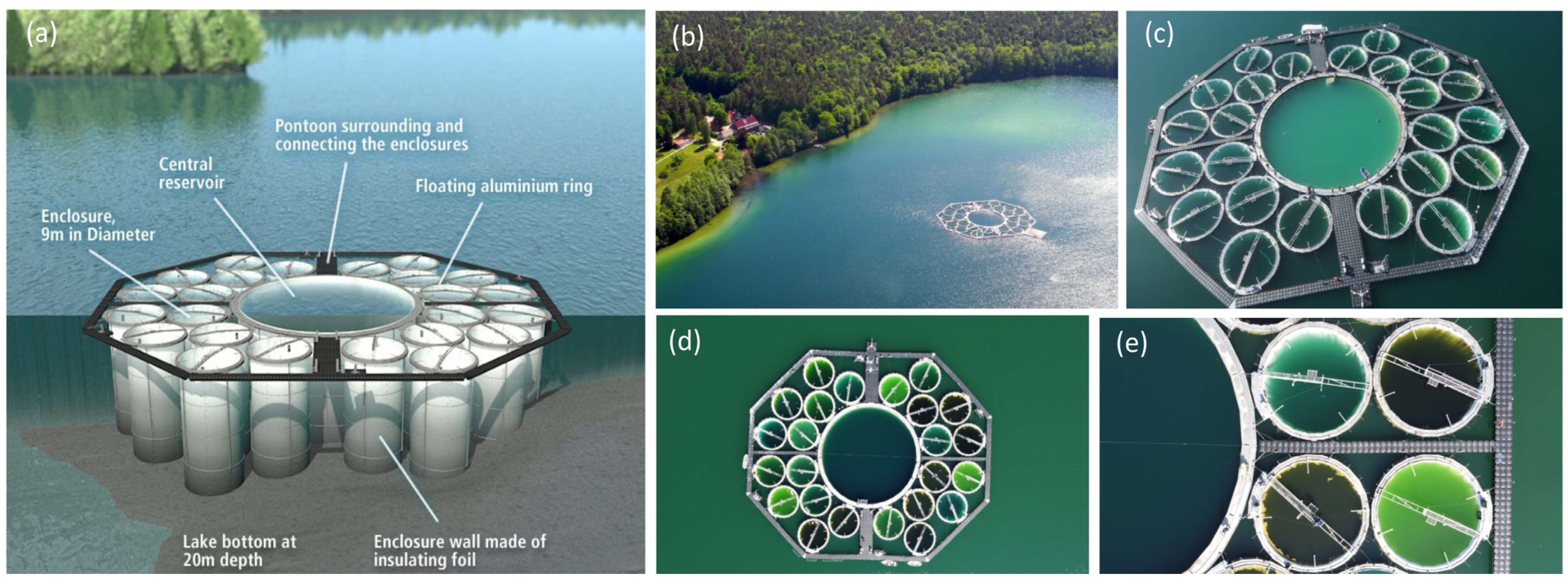

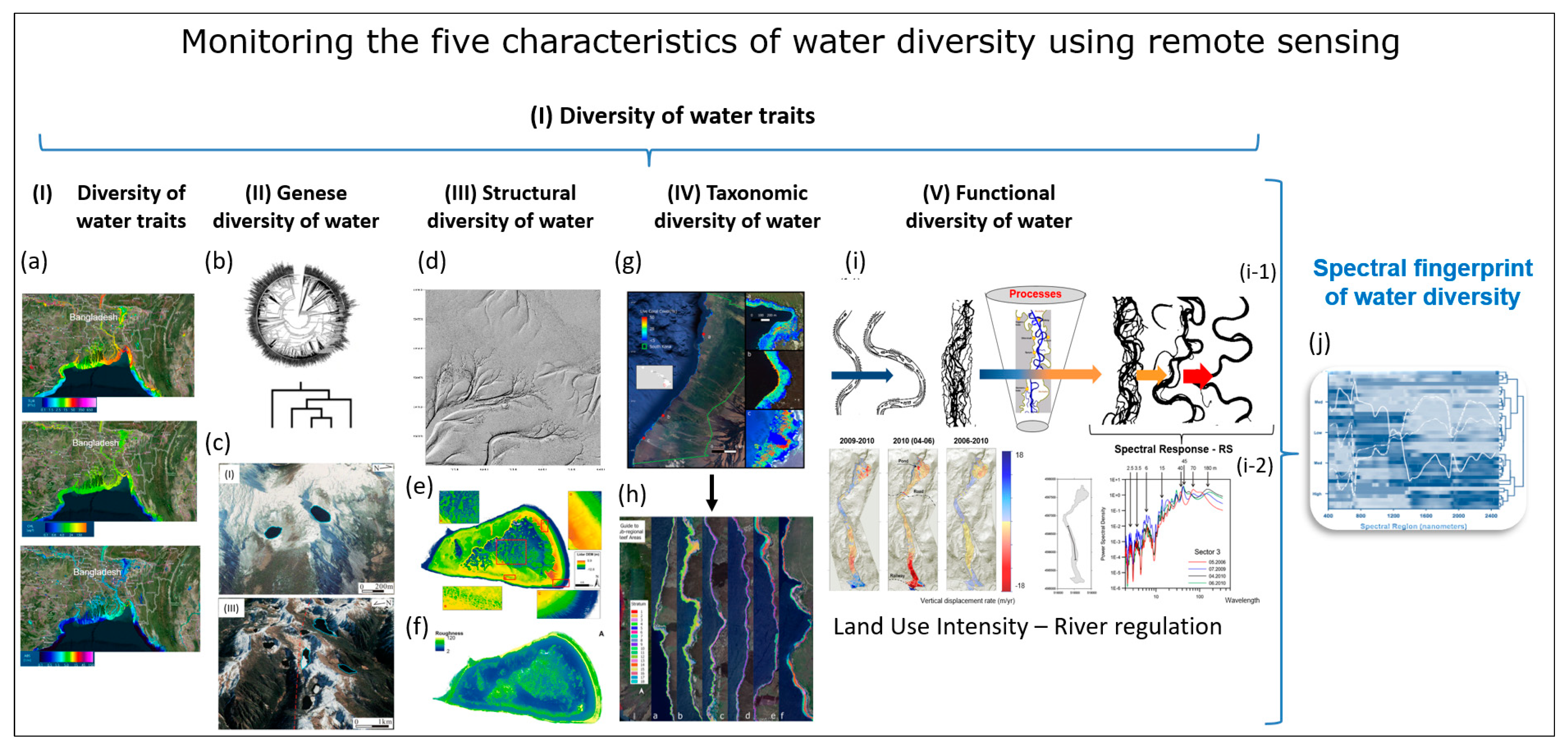
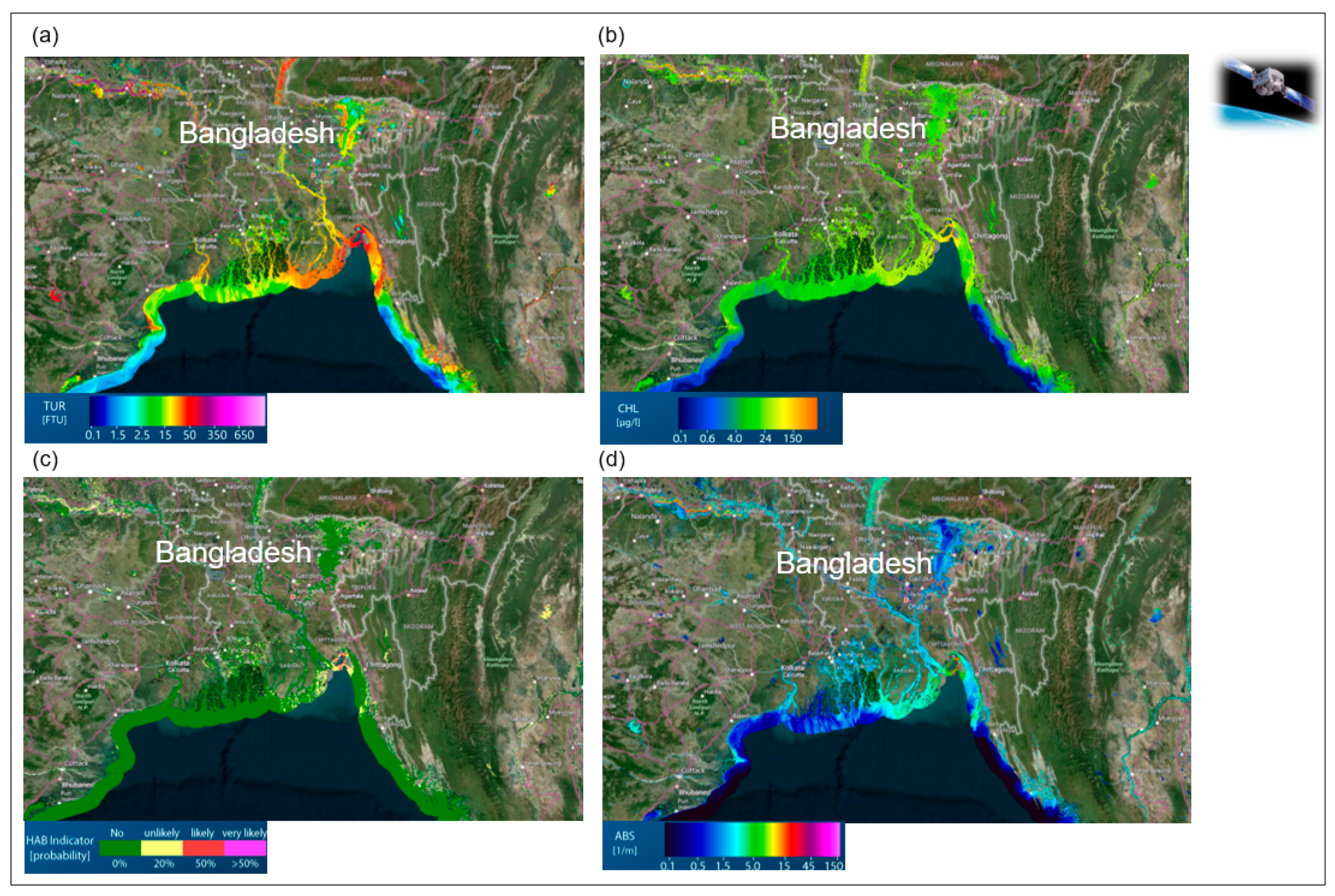
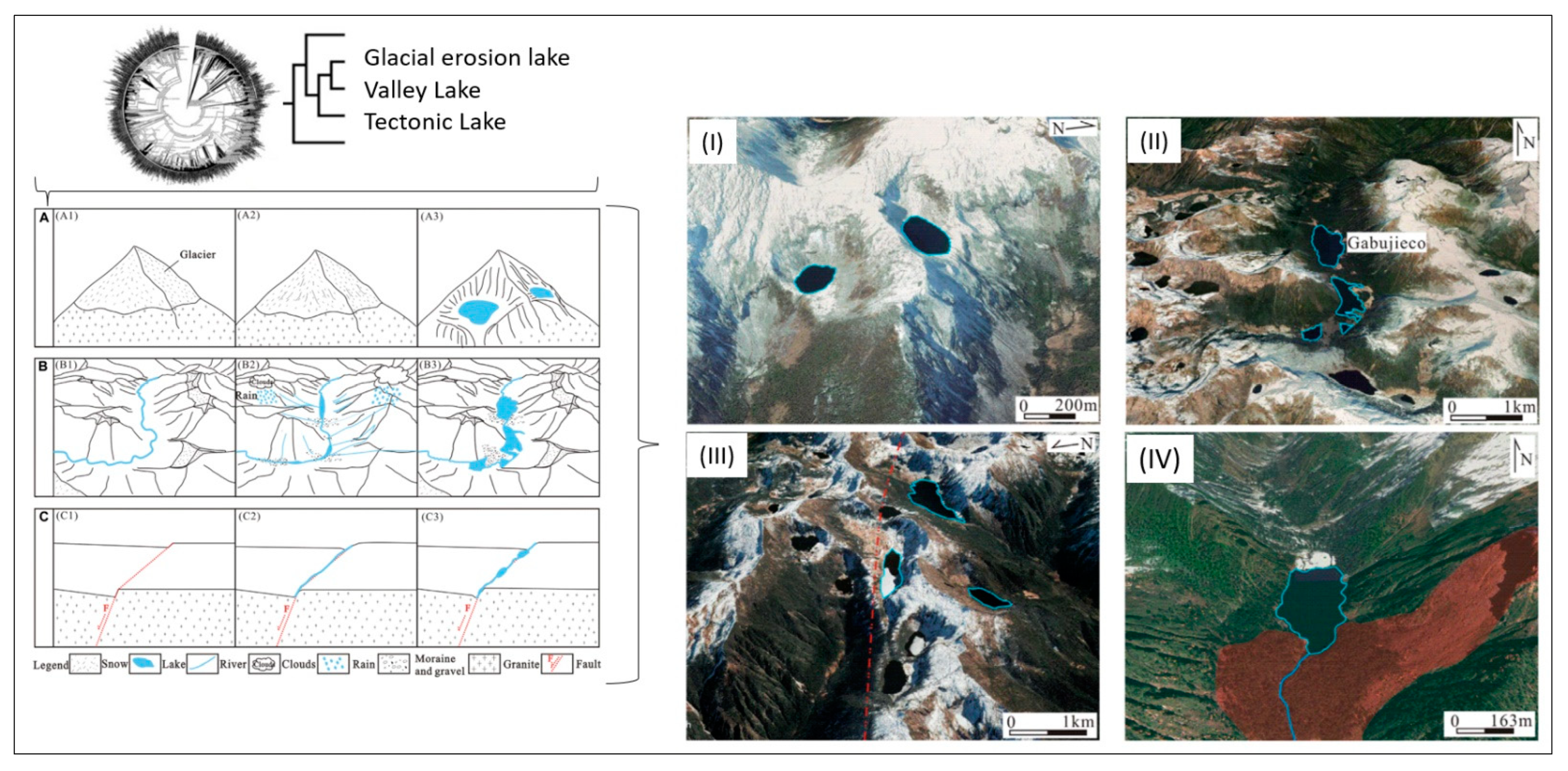
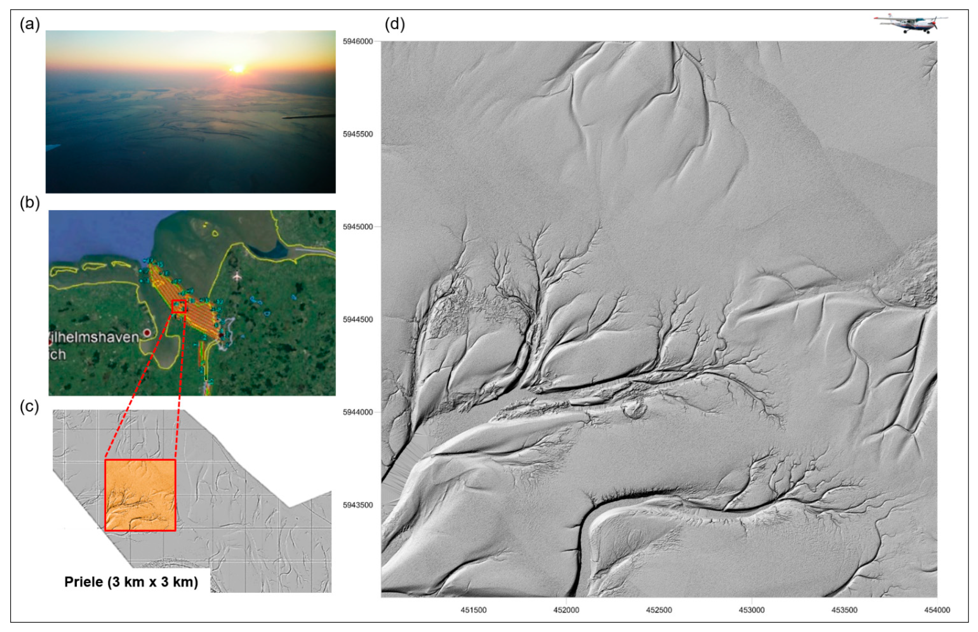
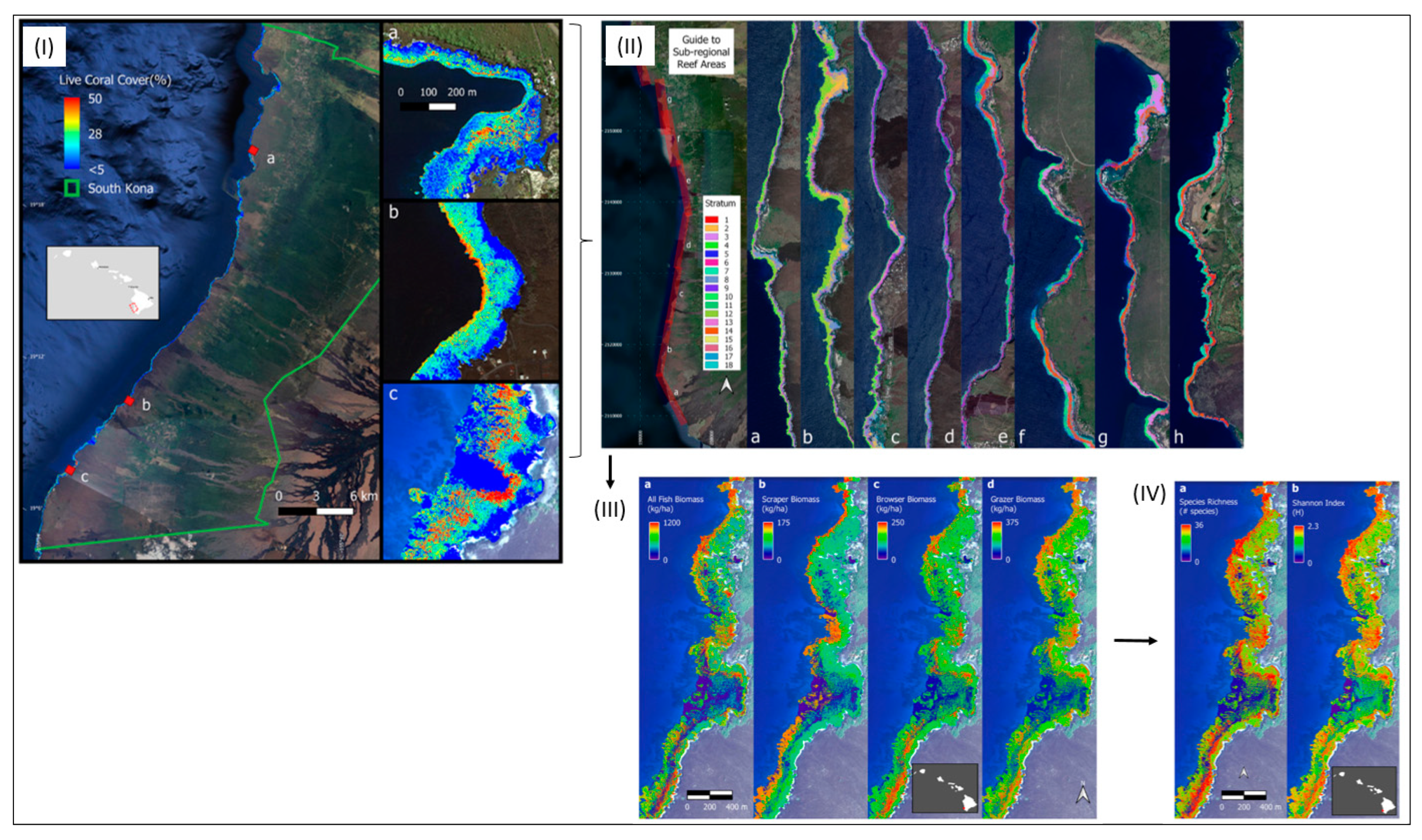
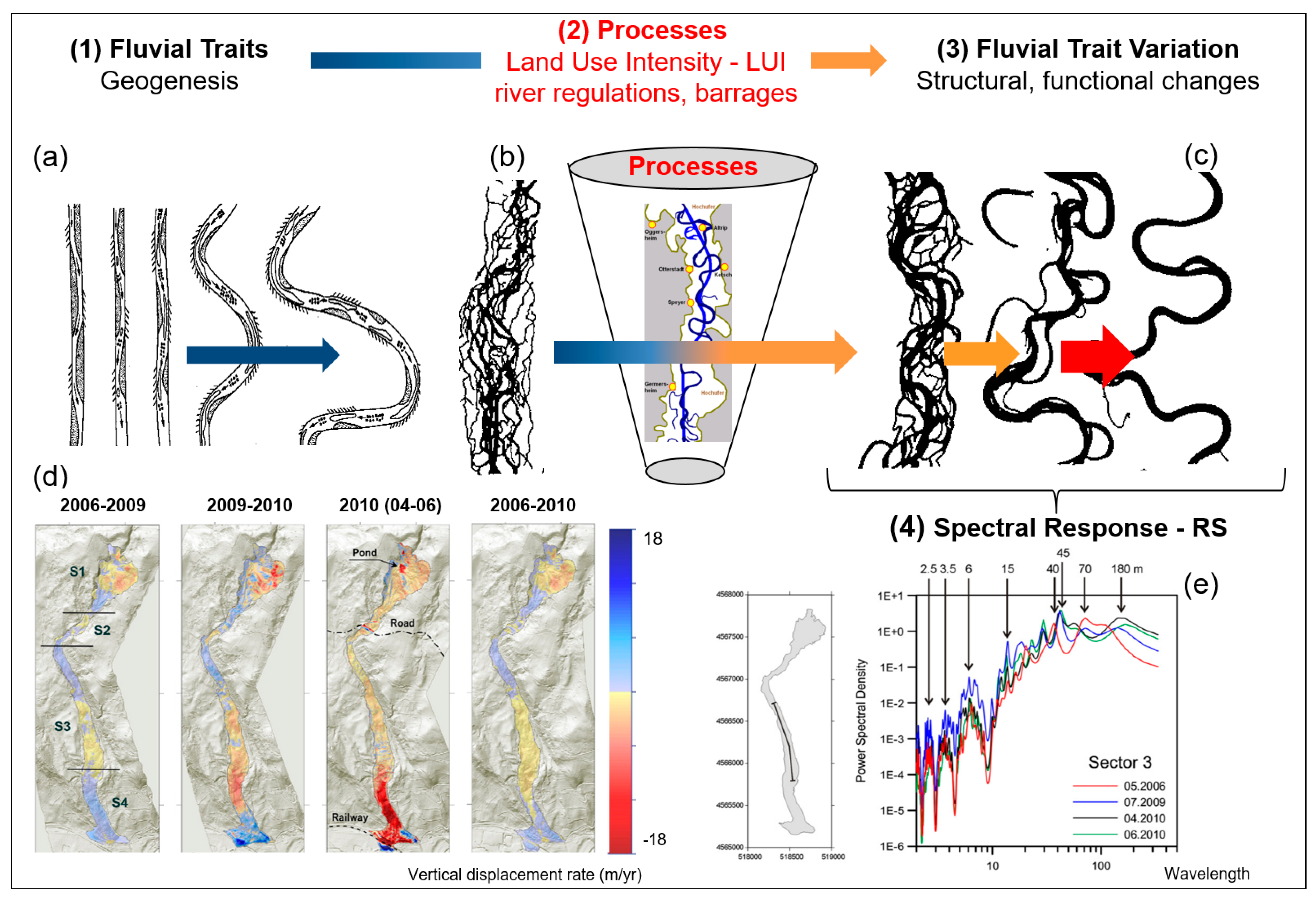
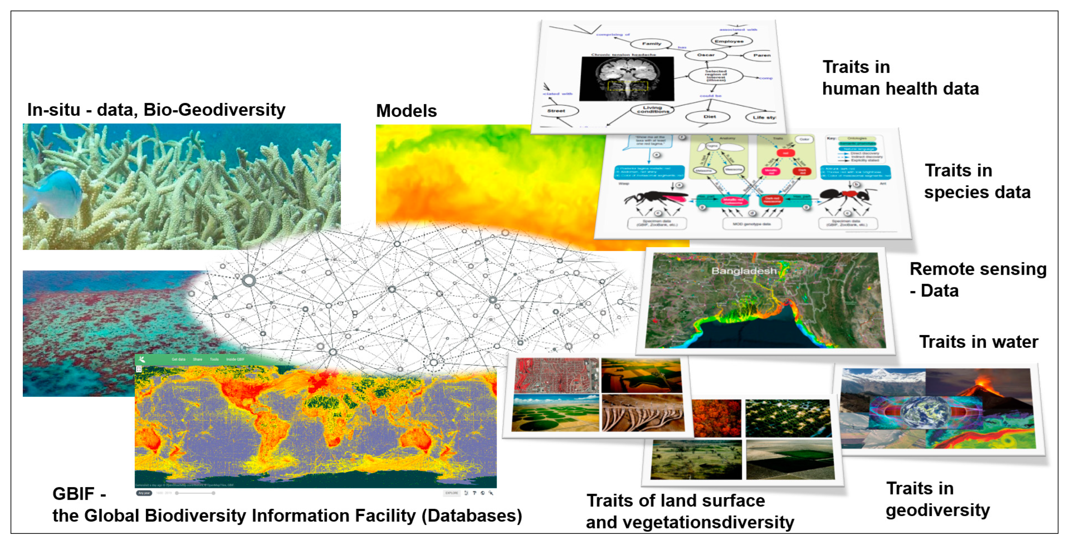
| Organisation | Guidelines | Link |
|---|---|---|
| World Health Organisation (WHO): |
| https://www.who.int/publications/i/item/9789241549950, accessed on 26 June 2024 |
| U.S. Environmental Protection Agency (EPA): |
| https://www.epa.ie/pubs/advice/water/quality/Water_Quality.pdf, accessed on 26 June 2024 |
| European Union (EU): |
| https://environment.ec.europa.eu/topics/water/water-framework-directive_en, accessed on 26 June 2024 |
| International Organisation for Standardisation (ISO): |
| https://www.iso.org/home.html, accessed on 26 June 2024 |
| American Public Health Association (APHA): |
| https://www.apha.org/, accessed on 26 June 2024 |
| European Union (EU) Water Framework Directive (WFD) |
| https://environment.ec.europa.eu/topics/water/water-framework-directive_en, accessed on 26 June 2024 |
Disclaimer/Publisher’s Note: The statements, opinions and data contained in all publications are solely those of the individual author(s) and contributor(s) and not of MDPI and/or the editor(s). MDPI and/or the editor(s) disclaim responsibility for any injury to people or property resulting from any ideas, methods, instructions or products referred to in the content. |
© 2024 by the authors. Licensee MDPI, Basel, Switzerland. This article is an open access article distributed under the terms and conditions of the Creative Commons Attribution (CC BY) license (https://creativecommons.org/licenses/by/4.0/).
Share and Cite
Lausch, A.; Bannehr, L.; Berger, S.A.; Borg, E.; Bumberger, J.; Hacker, J.M.; Heege, T.; Hupfer, M.; Jung, A.; Kuhwald, K.; et al. Monitoring Water Diversity and Water Quality with Remote Sensing and Traits. Remote Sens. 2024, 16, 2425. https://doi.org/10.3390/rs16132425
Lausch A, Bannehr L, Berger SA, Borg E, Bumberger J, Hacker JM, Heege T, Hupfer M, Jung A, Kuhwald K, et al. Monitoring Water Diversity and Water Quality with Remote Sensing and Traits. Remote Sensing. 2024; 16(13):2425. https://doi.org/10.3390/rs16132425
Chicago/Turabian StyleLausch, Angela, Lutz Bannehr, Stella A. Berger, Erik Borg, Jan Bumberger, Jorg M. Hacker, Thomas Heege, Michael Hupfer, András Jung, Katja Kuhwald, and et al. 2024. "Monitoring Water Diversity and Water Quality with Remote Sensing and Traits" Remote Sensing 16, no. 13: 2425. https://doi.org/10.3390/rs16132425