Abstract
High-frequency radars (HFRs) provide remote information on ocean surface velocity in extended coastal areas at high resolutions in space ((km)) and time ((h)). They directly produce radial velocities (in the radar antenna’s direction) combined to provide total vector velocities in areas covered by at least two radars. HFRs are a key element in ocean observing systems, with several important environmental applications. Here, we provide an assessment of the HFR-TirLig network in the NW Mediterranean Sea, including results from the gap-filling open-boundary modal analysis (OMA) using in situ velocity data from drifters. While the network consists of three radars, only two were active during the assessment experiment, so the test also includes an area where the radial velocities from only one radar system were available. The results, including several metrics, both Eulerian and Lagrangian, and configurations, show that the network performance is very satisfactory and compares well with the previous results in the literature in terms of both the radial and total combined vector velocities where the coverage is adequate, i.e., in the area sampled by two radars. Regarding the OMA results, not only do they perform equally well in the area sampled by the two radars but they also provide results in the area covered by one radar only. Even though obviously deteriorated with respect to the case of adequate coverage, the OMA results can still provide information regarding the velocity structure and speed as well as virtual trajectories, which can be of some use in practical applications. A general discussion on the implications of the results for the potential of remote sensing velocity estimation in terms of HFR network configurations and complementing gap-filling analysis is provided.
1. Introduction
High-frequency radars (HFRs) are shore-based instruments that remotely sense the surface ocean currents over extended coastal areas at high resolutions in space and time. They provide synoptic velocity maps reaching offshore distances of 30–200 km with a spatial resolution of 0.2–6 km depending on their emitting frequency, with a temporal resolution typically between 15 min and 1 h [1,2,3]. In the last few decades, they have become an essential worldwide component of coastal ocean observing systems [4,5] thanks to their extensive near real-time spatial coverage that provides an invaluable dynamical framework to other more localized in situ observation platforms [6,7]. In addition to surface currents, HFRs also provide derived wave and wind measurements that show significant potential, although they have not yet been adopted widely for operational monitoring [2,8,9,10]. HFR data play an essential role in addressing environmental and societal problems and applications. These include environment conservation and fishery management through an understanding of the larvae transport in the surface layer; pollutant mitigation through the reconstruction of pollutant dispersion and retention, for instance, in the case of oil spills; coastal management, for instance, through monitoring the impact of port activities on marine protected areas; maritime security, in support of Search and Rescue (SAR) operations and vessel navigation; and other emerging applications such as the monitoring of extreme events, tsunami detection, and ocean energy production [11,12,13,14,15,16].
The presence of spatial and temporal gaps in radar coverage remains a critical issue to address when using HFR data, especially for Lagrangian applications and including trajectory computations. Such gaps are almost unavoidable in long time series with extensive coverage. They are due to several environmental and technical reasons, such as interference, reflections, sea state (adverse conditions or insufficient sea surface roughness), and the occasional malfunctioning of the equipment or communication system [2,17,18,19]. As a consequence, an effective operational system is expected to provide not only raw and quality-controlled data but also gap-filled data to be used for practical applications. Various approaches have been proposed in the literature, including optimal interpolation [20], artificial neural networks [21,22], self-organizing maps (SOMs) [23,24], the variational method [25], several methods based on empirical orthogonal functions (EOFs) [15,26,27], and open-boundary modal analysis (OMA) [12,28,29]. OMA has been widely used because it is based on a set of modes that only depend on the geometry of the boundaries and, therefore, can be set up and used directly when installing an HFR system without the need for a long time series. Even though the comparisons with other methods indicate that OMA results can be outperformed [24], the simplicity of the setup often makes it the method of choice in operational systems.
This paper presents an HFR network in the northwestern Mediterranean Sea (NW Med), whose data are gap-filled using OMA. The system covers an area between the Corsica Channel and the Ligurian shelf in the coastal region in front of the cities of La Spezia and Viareggio (Figure 1). It is an important area from an environmental point of view as it includes many Marine and Coastal Protected Areas. In particular, it is inside the Pelagos Sanctuary, which is a Specially Protected Area of Mediterranean Importance (SPAMI) for the protection of marine mammals. The area also includes the Cinque Terre National Park and MPA, and the Porto Venere Natural Regional Park and MPA.
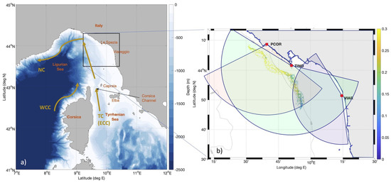
Figure 1.
(a) The study area with the Tyrrhenian and Ligurian basins and the main circulation patterns (NC, WCC, and TC). Blue colors show EMODnet 2022 bathymetric data (https://emodnet.ec.europa.eu, accessed on 30 June 2024). The black rectangle shows the area in the right panel; (b) close-up showing the coverage map of the three radar stations along with their locations and the drifter trajectories color-coded according to their speed (m/s).
Here, the HFR network performances were estimated by comparing the remote-sensed velocities from HFRs with the in situ velocities from surface drifter data, similar to what has been conducted in several previous studies for other HFR systems [30,31,32,33]. We used 40 drifters for a period of 3 days launched in the framework of a dedicated experiment during May 2019 (Figure 1).
The network, called HFR-TirLig, comprises three HFR stations, but, during the time window of the drifter experiment, only two of the three stations were operational. Consequently, information only from one station was available in part of the domain, so the total vector velocities could not be directly computed. This provides the opportunity to test the performance of the OMA gap-filled fields in a rather extreme case, where the vector velocity was computed based on a single station. Since this situation is not uncommon in practical applications, the results are relevant and expected to provide new and interesting insights.
2. Materials and Methods
2.1. Area of Interest
The area of interest is in the Northwestern Mediterranean, namely in the Ligurian Sea (LS), which is connected to the Tyrrhenian Sea by the Corsica Channel (Figure 1a). The LS is one of the most dynamic areas of the Mediterranean, dominated by the Ligurian or Northern Current (NC), a large-scale cyclonic circulation, active all year round flowing westwards along the coast [34,35]. A high mesoscale activity associated with meanders in the NC, eddy formation, or displacements of its core can be observed especially during the more energetic and cold season [36,37].
The NC originates north of the Corsica Channel from the merging of two other distinct currents: the Eastern Corsica Current or Tyrrhenian Current (TC), which flows along the eastern Corsica shores and through the Corsica Channel, and the Western Corsica Current (WCC), which flows along the Western Corsica coasts [38]. The variability of the Northern Current is mainly ascribed to the TC, which shows a marked seasonal cycle with stronger transport through the Corsica Channel during winter [35,39]. Currents are instead weaker, and water mass transports through the channel to near-zero values in summer [40].
The LS may be divided into two distinct zones. The western one is characterized by a northeast–southwest axis orientation of the Ligurian coastline, narrow shelf width, and deep bathymetric values exceeding 2500 m. The eastern one is shallower (depth for the Corsica Channel sill of about 450 m) for the presence of a much wider Tuscanian shelf and with a southeast–northwest axis orientation.
The area of interest lies exactly at the intersection of these two zones in the coastal region in front of the cities of La Spezia and Viareggio (Figure 1b). Dynamically, the area is both influenced by the large-scale Northern Current, especially when its core and meanders are pushed towards the coastline by southwesterly (Sirocco) winds [41], and by typical local coastal processes like the Arno River discharge, which creates the conditions for coastal fronts [42,43]. In this area, coastal currents spread in the south along the Tuscanian wide shelf, usually accelerating as they are squeezed in gradually narrower shelf waters when moving northward towards the Ligurian zone.
2.2. HFR System
At the time of the drifter experiment analysed here, the HFR-TirLig network was composed of three stations (Figure 1b), each of them hosting a Codar SeaSonde HFR system operating at a central frequency of 26.275 MHz and measuring the radial component of the surface ocean current.
Table 1 lists each HFR system’s exact location and operating parameters during 2019, the year of the drifter experiment.

Table 1.
Locations and operating parameters for each HFR station.
VIAR station is located in the port area of Viareggio and is hosted inside a lighthouse. To mitigate the influence of some conductive elements present in the surroundings (poles and fences), the HF antenna is placed about 10 m above the ground. Depending on the direction, the distance from the sea is between 50 and 150 m.
The TINO station is hosted inside the lighthouse on Tino Island, with the HF antenna towering above the structure. The elevation is 90 m above the sea level, and the horizontal distance from the sea is 50–150 m, depending on the direction. Since the radar is located on an island close to the mainland, sea echo from the first radial bins comes from an angular range of 270 degrees.
PCOR station is located on a little mound protruding into the sea, with an elevation of around 5 m and a distance from the seawater of around 10 m, in a rural area on the edge of the urban area of Monterosso al Mare town. The surrounding hills limit the angular measuring range to about 100 degrees; however, they help shield the radar from disturbances originating from land.
All the above SeaSonde HFR systems are equipped with a single transmitting and receiving vertical monopole and two horizontal colocated receiving antennas, resulting in an extremely compact design. Codar SeaSondes are Direction-Finding-type radars; i.e., they acquire, for a given radial distance, the backscattered signal coming from all the azimuth simultaneously, and then they estimate the direction of arrival (DOA) of each contribution (sea echo from each patch of the ocean along the circle at a given distance from the antenna).
The signal analysis is performed through the proprietary software Codar SeaSonde Radial Suite, version 7 which implements an optimized version of the general MUltiple SIgnal Classification (MUSIC) algorithm [44,45,46]. Each HFR system can only estimate the radial component of the current velocity. All the radial velocities in the present paper are calculated by the Codar SeaSonde Radial Suite v7. 10R7-Update4 with the following settings: Raw cross spectra files (CSQ) are 64 range cells by 512 Doppler bins; cross spectra short time files (CSS) are averaged over 15 min and output every 10 min; radial processing is enabled with ideal and measured pattern for 75 min average and output every 60 min, using 5-degree resolution with a range up to 44.730 km.
The response (amplitude and phase) of the radar’s receiving antenna elements as a function of the angle in the horizontal plane, the so-called receiving antenna pattern, provides crucial information to the MUSIC algorithm for estimating the DOA of radial velocities. Two options are available for this pattern: using the so-called “ideal” or “measured” pattern. The “ideal” antenna pattern refers to the theoretical response of the receiving HFR antennas and is well-known for Codar HFR systems. The real response of the receiving HFR antennas, once they are placed in the field, can be, however, significantly altered with respect to the ideal case, and distortions in amplitude and phase could be introduced. For this reason, the calibration of the receiving antennas, also called (receiving) antenna pattern measurement (APM), and the use of a “measured” antenna pattern is a standard procedure generally recommended [5,17]. It is possible that, in some cases, in the presence of distortions, the measured pattern could worsen the estimates [47,48]. For this reason, validation exercises are necessary to assess to what degree the use of the measured antenna pattern provides better results with respect to the case of the ideal pattern.
All HFR-TirLig radar systems were installed and maintained following as much as possible the recommendations provided by the literature [5], including the antenna calibration, and, in the following analysis, results from both ideal and measured patterns are compared. We point out that the antenna response affects the DOA estimation so that the angular distribution over the HFR coverage of radial velocities may differ if calculated with measured pattern with respect to the case of ideal pattern [49]. This will be evident in Section 3, when the number of radials available for comparison with drifter velocity for some range cells will differ in the two cases. Once the radial velocities are estimated, total vector velocity fields are calculated by combining the radial components of two or more HFR systems over a regular grid in the overlapping measurement area.
All velocities produced by the HFR-TirLig network are processed in near real-time within the European HFR Node workflow [2]. Radial velocities estimated by the network, hereafter referred to as , are quality controlled and integrated into interoperable datasets according to the European standard QC, metadata, and data model [50]. Furthermore, values are combined to estimate the total velocity in the areas where the coverage ranges of at least two radial stations overlap. The total velocity estimates, referred to hereafter as , are also quality controlled and integrated into interoperable datasets according to the European standard QC, metadata, and data model [50]. The combination process performed by the European HFR Node is based on the open source HFR_Progs Matlab library (https://github.com/rowg/hfrprogs (accessed on 30 June 2024) [51]) that applies the unweighted least squares fitting (UWLS) algorithm [52,53,54]. The resulting total velocity fields are produced with a grid size of 2 km.
Radial velocity data and total vector velocity data produced by the HFR-TirLig network are freely available on the THREDDS Data Server of the European HFR Node (https://thredds.hfrnode.eu, accessed on 30 June 2024) at the “Tyrrhenian_Ligurian_Sea” catalogue (https://thredds.hfrnode.eu:8443/thredds/NRTcurrent/HFR-TirLig/HFR-TirLig_catalog.html, accessed on 30 June 2024) and are distributed via the Copernicus Marine In Situ TAC (http://www.marineinsitu.eu/, accessed on 30 June 2024), EMODnet Physics (https://emodnet.ec.europa.eu/, accessed on 30 June 2024), and SeaDataNet (https://www.seadatanet.org/, accessed on 30 June 2024) data portals.
At the time of the drifter experiment, the PCOR station was under maintenance due to electronic failure. Thus, the effective coverage of the HFR network was reduced to the overlapping area between TINO and VIAR stations only, corresponding to the area between La Spezia and Viareggio.
2.3. OMA Gap Filling
Open-boundary modal analysis (OMA) [29,55] is widely used to fill spatiotemporal gaps in HFR measurements. The power of the OMA method consists of its ability to incorporate the flow across open boundaries so that, differently from other modal analysis techniques [56,57], no a priori knowledge of the normal velocity at open boundaries is needed. The output of the OMA method is a set of time and data-independent eigenfunctions (modes) that can be used to interpolate velocity fields on arbitrary domains, allowing fluxes through selected segments of the boundaries. These modes only depend on the geometry of the boundary and do not change in time. This means that their computation must not be completed at each time-step, but they can be evaluated once and then stored for future uses, thus making this technique ideal for real-time applications. The resulting modes are linearly independent and are grouped as interior and boundary modes. The interior mode set is composed of incompressible modes (i.e., divergence-free) and irrotational modes, while the boundary modes are obtained by solving the singular but consistent Neumann problem. The union of the interior and boundary modes builds a complete functional basis where the flows can be projected for realizing the gap-filling of the total velocity field. OMA method considers the kinematic constraints imposed on the velocity field by the coastline (modes are calculated considering the coastline by setting a zero normal flow). Depending on these constraints, they can be limited in representing localized, small-scale features as well as flow structures near open boundaries [29].
The setup of the OMA framework for the analysis described in this paper was performed in three steps: (i) the construction of the domain, (ii) the evaluation of the modes, and (iii) the projection of radial velocities measured by the HFR systems onto the OMA modes to obtain the OMA gap-filled total velocity fields .
The domain for implementing the OMA method for the HFR-TirLig network was built based on the complete dataset of HFR total velocity fields measured by the HFR systems during 2019. In particular, the domain was selected as the set of the grid cells in the HFR network coverage where total velocity vectors were present for at least 50% of the time during the year 2019, as shown in Figure 2.
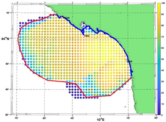
Figure 2.
Selection of the domain for the application of OMA method. The grid cell colors represent the percent coverage in time of the total velocity vectors measured by the HFR network from 1 January 2019 to 31 December 2019. The open boundary is painted in red, and the closed boundary is painted in blue.
The entire boundary, composed of the closed boundary (blue line in Figure 2) and the open boundary (red line in Figure 2), was smoothed to a 500 m linear resolution.
The OMA modes were generated by using the HFR_Progs Matlab open library [51]. Further, 214 interior modes and 104 boundary modes were created.
The gapfilled total velocity fields were then obtained by fitting the radial velocity fields measured by the PCOR, TINO, and VIAR antennas on the modes described above. The fit is performed using the HFR_Progs Matlab open library [51].
We recall that, during the drifter experiment (i.e., May 2019), the PCOR station was down due to some electronic failure. During this period, the total velocities provided by the HFR-TirLig network were computed only in the area between La Spezia and Viareggio that both TINO and VIAR sampled (see an example of daily averages in Figure 3a), whereas the OMA velocities were still computed on the total domain (Figure 2), as shown in Figure 3b. The velocities in the northern part of the domain were based only on the TINO radials. In the following, we will refer to the complete OMA domain in Figure 2 as F, i.e., the Full domain, while we also define two sub-domains that will be used in the diagnostics presented in Section 3. The Observation sub-domain (hereafter referred to as O and shown in yellow in Figure 4) is defined as the set of the grid cells of the HFR network coverage where total velocity vectors were present for at least 40% of the time during the two months of May and June 2019. The 40% threshold has been chosen as a compromise between acceptable data coverage and sufficient spatial coverage to include the drifter tracks. Sensitivity tests with coverage show consistent results but reduced number of available drifter data. The second sub-domain (shown in red in Figure 4) is the difference between the Full and Observation domains, hereafter referred to as sub-domain F–O. In the F–O sub-domain, only radial velocities measured by the TINO station are present; i.e., no total vector velocities can be computed directly from radar measurements.
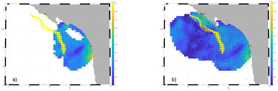
Figure 3.
Comparison of the daily-averaged combined total velocity field (a) versus the daily-averaged OMA gap-filled total velocity field (b) on 3 May 2019. The tracks of the drifters released during the experiment are superimposed in yellow. The gap in the combined velocity field is due to a poor geometry along the baseline between TINO and VIAR stations, i.e., high GDOP values filtered out by the QC procedures. This gap is filled by the OMA technique in the right panel.
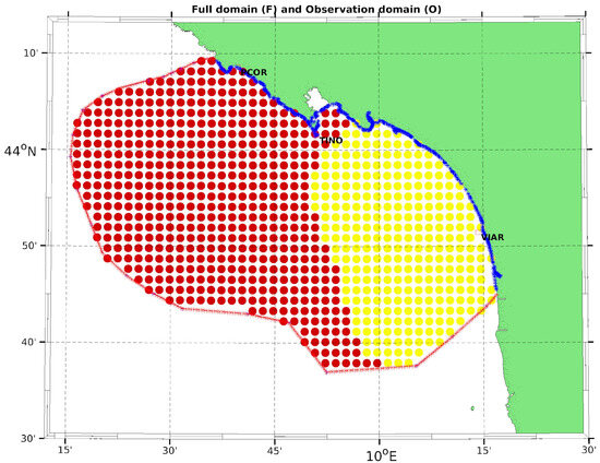
Figure 4.
Domains used for comparison between HFR velocity fields and drifter velocities. The O sub-domain is highlighted in yellow, while the F–O sub-domain is highlighted in red. The union of the two domains, i.e., yellow plus red, is the F domain.
2.4. Drifter Data
The results of the HFR system were compared with velocities measured by CARTHE drifters (Consortium for Advanced Research on Transport of Hydrocarbon in the Environment, [58]). They are mostly biodegradable, low-cost drifters designed to sample the ocean currents in the upper 60 cm. They have been tested to obtain high-accuracy observations of horizontal velocity, reducing wave rectification and wind slip velocity (<0.5% with respect to wind speed [58]).
A total of 40 CARTHE drifters were launched in the area of interest on 2 May 2019 (Figure 1b) in the framework of the IMPACT project (https://www.seanoe.org/data/00612/72369/, accessed on 30 June 2024). Most of the drifters were launched in the open sea facing Viareggio and La Spezia on a regular grid (about 6 km side with 1 km step) in a time window of about 2–3 h, while 5 drifters were released along a line from the mouth of the La Spezia Gulf to the open sea. Upon launching, all drifters moved in the general northwestward direction following the boundary current (Figure 1) and stayed in the coverage domains of the HFR system (cf. Figure 3 and Figure 4) for approximately 3 days.
In the southern part, corresponding to the wide Tuscanian shelf area in front of Viareggio, velocities are around 0.1–0.15 m/s. More to the north, as the shelf narrows approaching the Ligurian one, currents accelerate, exceeding m/s.
The drifters were equipped with GPS receivers gathering position data every 5 min with an accuracy of approximately 5–10 m. Drifter positions were processed for removing outliers and spikes, and velocities along trajectories were computed by central finite differences of the positions.
2.5. Considerations on Drifters and HFR Data Comparison
Drifters provide accurate in situ information on current velocities covering extensive areas and are relatively affordable and simple to deploy. They are, therefore, very apt to be used for comparison with spatially extended, remotely obtained HFR data, and, indeed, they have been widely used in this capacity in past decades [30,31,32,33]. It should be noted that there are intrinsic differences between the two types of instruments and samplings, so a complete match between drifter and HFR data cannot be expected.
In the vertical, depending on drogue and design, drifters can sample from the very first few centimetres to 15–20 m from the surface [59], while the exponentially weighted vertical averaging of HFR occurs over the entire water column and results (in our case) in an effective measurement depth of , where is the transmitted wavelength [60,61,62]. In the case discussed here, vertical sampling is roughly compatible between the two types of instruments [63] given that CARTHE drifters sample the upper 60 cm and the HFR system has a working frequency of 25 MHz with an effective sampling depth of approximately 50 cm. On the other hand, inherent differences cannot be eliminated in the horizontal. Drifters sample the environment at their own scale, which is less than 1 m in the case of CARTHE, while HFRs provide average quantities at scales of a few km resolution [30]; in our specific case, total vectors are calculated at 2 km horizontal resolution. Considering the above spatial resolution properties and the respective sampling frequency, 1 h for HF radar data and (nominally) 5 min for CARTHE drifters, the drifters sample the variability within the radar cells, including many submesoscale and turbulent processes typically characterized by high shears. These processes are averaged within the radar cell, so a satisfactory comparison has to be within the range of expected variability in the horizontal grid [30]. While a quantitative estimate of such variability is typically not available, results from the literature provide general guidance suggesting that discrepancies of the order of 5–20 cm/s can be considered acceptable, depending on the radar emitting frequency and on the energetics of the area under examination [2,14,31,32,33,47,63,64,65,66,67,68]. In this framework, it is useful to consider the ratio of the difference between the two measurements and the actual in situ velocity measured by the drifters . Ratios in the order of 0.5 typically indicate satisfactory results within the bounds of expected variability.
2.6. Metrics and Strategy of Comparison
2.6.1. Eulerian Comparison
The comparison between HFR and drifter-derived velocities is first performed in an Eulerian framework, i.e., using several metrics and configurations where HFR and drifter information are taken at the same times and locations. This is achieved in time by resampling drifter data on the hourly uniform radar time grid and in space by estimating radar velocities at the drifter positions using bilinear interpolation of the velocities corresponding to the closest cells. For each pair of HFR and drifter data corresponding to the same time and position, differences are computed and characterized using standard metrics. All statistics are computed using both the measured and ideal antenna patterns for comparison.
The analysis is first performed considering radial velocities since they provide the most direct measurements from the remote radar system. Radial velocities from the two available HFR stations, , are compared with projected drifter velocities along the radial directions . The difference is computed for all available pairs, and the statistics are characterized in terms of bias and root mean square (RMS) , where stands for the average operator. RMS is also computed based on drifter velocities only for reference, , and is used in the ratio with , to provide a normalized measure with respect to the environmental variability, as discussed in Section 2.5. Correlation coefficients at zero lag are also computed between time series from HFR and drifters.
Total vector velocities are then analyzed in terms of components and speed U, where . While the two velocity components provide a specific vector assessment, the speed is an effective bulk indicator used in previous studies of velocity estimates [69]. Statistics are computed as for the case of , considering differences for speed and , for the two components.
For these analyses, different configurations and domains are considered. In the Observations (O) sub-domain (Figure 4 yellow dots), where both TINO and VIAR stations provided coverage, HFR-based vector velocities were first computed using the standard methodology in Section 2.2, without applying any gap filling. These are the basic velocity products provided by HFR systems, and their assessment is very relevant for practical applications, also providing a “benchmark” for the gap-filled OMA results. The OMA method was then used to compute vector velocities over the Full (F) domain, and the results were analyzed separately in the (O) and (F–O) sub-domains. In the (O) sub-domain, the results from the OMA vectors can be directly compared with the results. In (F–O) (Figure 4 red dots), on the other hand, only vector velocities are available. The results in this domain depend on radials from only one HFR system and on the kinematic filling built by OMA, therefore providing a very stringent test of the methodology. Finally, we consider results for over the whole (F) domain to characterize the general performance of the system during the period of interest. Therefore, we are considering 4 different configurations for each parameter and metric, as better detailed in the following.
2.6.2. Lagrangian Comparison
As a second step, a Lagrangian framework is considered by comparing trajectories from the observed (real) drifters (RDs) with virtual trajectories (VDs) computed from HF radar velocities, following similar examples by [14,31,70,71,72]. Lagrangian diagnostics are especially relevant for practical applications involving the prediction of surface drift and provide an integrated performance assessment since the error is integrated in time.
The VDs are computed using the gap-filled OMA hourly surface velocity fields using a fourth-order Runge–Kutta scheme for the integration process. Two configurations are considered. The first one considers the O domain, where VDs are initialized at the RD’s deployment location and then tracked until they exit the domain. In the second configuration involving the F–O domain, VDs are initialized at the locations where the RDs enter the domain and tracked until they exit. In both cases, the drifter data are interpolated to match the radar timestamps, and the separation distance, d, between the virtual and observed drifter locations is computed at hourly intervals. This separation distance serves as a first indicator of the HF radar network’s performance, with smaller values of d indicating better performance. A value of d = 0 signifies perfect performance, where the virtual drifter coincides exactly with the actual drifter’s position.
Following [72,73,74,75], we also estimate the Skill Score (SS), based on the Normalized Cumulative Lagrangian Separation (NCLS) distance between virtual and observed drifter trajectories, in both O and F–O sub-domains. The normalized SS and NCLS metrics allow us to compare results obtained in areas characterized by different energetics, and they have been used to quantify model performances in a wide range of applications in the context of oil spill management and SAR [76,77,78]. The NCLS distance, introduced by [73], is defined as the cumulative sum of the separation distances between virtual and observed trajectories d, weighted by the cumulative length of the observed trajectory over time, as follows:
where is the separation distance between observed and virtual trajectories at time-step i, while is the length of the observed trajectory at the same time-step, and M is the total number of time-steps (or forecast horizon). The NCLS can estimate the relative performance of the HF radar system in different current areas, but it is unconventional compared to traditional Skill Scores. A lower NCLS value indicates better radar performance, while a higher value in conventional Skill Scores means better performance. Thus, the use of a similar Skill Score was also introduced: the SS index
where n is a non-dimensional, positive number that defines the threshold of no skill (SS = 0). In the following, as in several previous applications [75], we choose .
3. Results for Eulerian Comparisons
3.1. Radial Velocities
The results for the radial velocities are summarized in Table 2 and Figure 5 for the two active stations, TINO and VIAR. In the following, we first review the results obtained with the measured antenna patterns and then discuss the differences with the ideal pattern.
Table 2.
Statistical results for radial velocities () obtained comparing radar - and drifter -based velocities for TINO and VIAR stations. Values evaluated for ideal radial velocities are reported in parentheses.

Figure 5.
Comparison between radar and drifter radial velocities for the two stations: VIAR upper panels; TINO lower panels. Scatterplots (a,c) and locations (b,d) of the compared pairs are shown for VIAR and TINO, respectively, color-coded according to the absolute difference between radar and drifter velocities. The coefficients a and b in the insets indicate the slope and intercept of the scatterplot regression lines.
The VIAR system covers the southern part of the drifter trajectories (Figure 5b) where the velocities are reduced (Figure 1) and the radial velocities with m/s characterize the area. The number of hourly HFR and drifter data pairs, N = 224, is relatively low due to occasional gaps in space and time in the area of the drifters, situated close to the radar’s maximum range. The RMS difference between the HFR and drifter radial velocity is m/s, which corresponds to a ratio with respect to the drifter estimate, . The bias is negligible, and the correlation coefficient (with confidence intervals CI 95%, (0.76, 0.85)). The statistical results indicate a good agreement between the drifter and the radial HFR datasets.
The TINO coverage is more extended (Figure 5d), with substantially more data pairs (N = 2122) and with radial directions more aligned with the trajectories, also including the more energetic northern part of the domain ( m/s). Consequently, the values of and are more than double with respect to VIAR. The and the correlation coefficient is (0.85, 0.87 CI), however, are similar to VIAR, indicating a similar positive performance for the two HFR systems, even though a significant bias is observed for TINO, m/s. The scatterplots shown in Figure 5a,c emphasize the different velocity scales recorded by the two antennas and reflect the slightly reduced performance of TINO, probably due to the high differences in the northernmost part, close to the HFR system outer range (Figure 5d). Overall, the results are well within the typical accuracy of HFR systems, as shown by the range of statistical values reported in the literature for similar comparisons [14,32,33,79].
The ideal pattern values (reported in parentheses in Table 2) are qualitatively similar but slightly worse, with higher RMS and lower correlations, in line with what is expected.
3.2. Total Vector Velocities
We start presenting the results for the total velocities estimated by the HFR-TirLig network where the measurements from the two stations are available, i.e., in the O sub-domain, using the standard method discussed in Section 2.2 without gap filling. We then consider the gap-filled results in the two sub-domains, O and F–O, and the total domain F.
3.2.1. Velocities in the O Sub-Domain
The statistical results, summarized in Table 3 and Figure 6a,b, are based on N = 601 pairs for the measured pattern. We notice that this is more than double the pairs in the VIAR radial velocity statistics (Table 2) as the greater coverage can also be observed in Figure 6b with respect to Figure 5b. This is because the total vector velocities are on a regular 2 km grid, while the radial grid depends on angle and range. In the area covered by the drifters, close to the maximum radar range, the cells of the radial grid are coarser, resulting in a smaller number of pairs.
Table 3.
Statistical results for total vector velocities obtained comparing radar and drifter -based velocities in terms of speed U and u and v components in the O sub-domain. Results obtained using ideal radials are reported in parentheses.
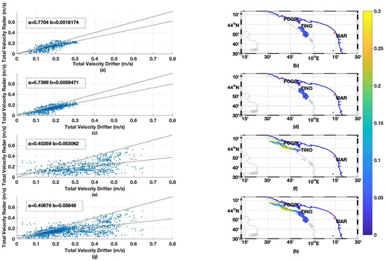
Figure 6.
Comparison between radar and drifter total vector velocities in terms of scatterplots (left) and locations (right) of the compared pairs color-coded according to the absolute difference between radar and drifter velocities. The coefficients a and b in the scatterplot insets indicate the slope and intercept of the regression lines: (a,b) for in O sub-domain; (c,d) for in O sub-domain; (e,f) for in F–O sub-domain; (g,h) for in F domain.
The speed U is relatively low in the O sub-domain, m/s, even though it is almost double the radial component velocity due to the angle between the radial and total velocities. The RMS difference between radar and drifter speed is m/s, leading to a with respect to the drifter estimate. The bias is m/s and the correlation coefficient (0.71, 0.78 CI). The results indicate a good agreement between the drifter and the HFR-based speed estimates.
Regarding the velocity components, the latitudinal v measured by the drifters is double the longitudinal u, while the values of are similar, resulting in a lower ratio for v, than for u and . The biases are m/s, m/s, and the correlations 0.69 (0.65, 0.73 CI) and 0.73 (0.69, 0.76 CI), respectively. The component comparison is more stringent than for speed, and it is therefore not surprising that the results slightly worsen with respect to U. Overall, they remain very positive and compare well with the results in the literature [30,33,80], confirming the good performance of the radar system.
The results obtained with the ideal patterns (reported in parentheses in Table 3) are similar to those obtained with the measured patterns but slightly worse for most statistics.
3.2.2. Velocities in the O Sub-Domain
The results for the gap-filled velocities in O are shown in Table 4 and Figure 6c,d. We recall that the O sub-domain is characterized by minimum temporal coverage of both HFR stations, implying that occasional gaps in time and space occur in the area, as is common in HFR systems. The OMA procedure fills these gaps, producing continuous velocity fields in space, , resulting in a number N = 834 of pairs where the statistics are performed. This number is significantly higher than the value for , (N = 601, Table 3) since the values are computed only in the grid cells with both radars’ coverage. Compared to the statistics (Table 3), the results are basically equivalent, even though small differences can be observed, slightly improving the more energetic v component and speed results while slightly worsening the less energetic u component. As for , the results obtained with the ideal patterns (reported in parentheses in Table 4) are slightly worse than for the measured patterns, especially for the u component.
Table 4.
Statistical results for total vector velocities obtained comparing OMA gap-filled and drifter -based velocities in terms of speed U and u and v components in the O sub-domain. Results obtained using ideal radials are reported in parentheses.
The results indicate that OMA is very efficient in filling occasional gaps, providing consistent, continuous fields without adding excessive smoothing.
3.2.3. Velocities in the F–O Sub-Domain
The results for in F–O are shown in Table 5 and Figure 6e,f. The F–O sub-domain is more extended than O (Figure 4), and it includes the northern area where the shelf narrows and the boundary current becomes more energetic, as shown by the drifter trajectories (Figure 1). Only information from the TINO system is available in this area, providing a very strict test for the OMA gap-filling.
Table 5.
Statistical results for total vector velocities obtained comparing OMA gap-filled and drifter -based velocities in terms of speed U and u and v components in the F–O sub-domain. Results obtained using ideal radials are reported in parentheses.
The statistics are computed over N = 846 pairs, covering the northernmost part of the trajectories (Figure 6f). The velocities are higher than in domain O, with approximately double ( m/s). The results for speed show an RMS difference with drifters m/s, corresponding to a ratio , and a correlation coefficient (0.43, 0.53 CI). This suggests an acceptable performance for speed, except for the high bias, m/s.
The two velocity components have similar , slightly more energetic for u ( m/s) than for v ( m/s), consistently with the trajectory directions. The comparison with the drifter components worsens with respect to the speed, showing increased ratios, and , respectively, and smaller correlations , ( (0.20, 0.32 CI) and (0.23, 0.35 CI), respectively, for u and v).
Overall, the performance is acceptable for speed but marginal for the components. The biases are high, as shown also by the scatterplot in Figure 6e, with underestimating the drifter velocities, especially for high values. On the other hand, given the very reduced information, i.e., only the TINO radials during the whole period of analysis, appears to still be able to provide some valuable information, at least partially reconstructing the energetics and the structure of the boundary current (see also Figure 3).
3.2.4. Velocities in Full F Domain
As a final step, we evaluate the performance of over the full domain F (Table 6, Figure 6g,h). The results combine those already discussed for the O and F–O domains, but it is interesting to provide a quantitative overview that includes the complete coverage of the HFR network.
Table 6.
Statistical results for total vector velocities obtained comparing OMA gap-filled and drifter - based velocities in terms of speed U and u and v components in the F domain. Results obtained using ideal radials are reported in parentheses.
The area of interest covers the full trajectory extent (Figure 6h), with N = 1680 and m/s. The overall performances for speed are characterized by and correlation (0.56, 0.62 CI), while, for the two components, the ratios reach and and the correlations (0.52, 0.58 CI) and (0.30, 0.38 CI) for u and v, respectively. The biases are high, as shown by the scatterplot in Figure 6g.
Overall, the whole system’s performance confirms that, in the absence of one HFR station, the use of a gap-filled can provide information that can at least partially describe the area of interest.
3.3. Graphical Summaries for the Eulerian Comparisons
In this section, we attempt to concisely summarize all the results of Section 3 using a graphical representation in the parameter space of the various metrics.
We start by considering the space spanned by the values of the zero-lag correlation between the radar and drifter estimates and the values of the RMS statistics of their difference , including all the variables (radial velocity , speed U, and velocity components u and v) and all the configurations, i.e., the three domains (O, F, and F–O) for both the ideal and measured antenna patterns. The results in Figure 7 show the importance of the different domains. Four different clusters can be identified: a first cluster gathers all the total velocity results in sub-domain O (red and blue circles), characterized by high correlation coefficients () and low ( m/s) for all the variables, with the only exception of the OMA u component in the ideal configuration. This first cluster shows that, in sub-domain O, where coverage is provided by two radars, the OMA and HFR totals are statistically comparable, and the use of the measured or ideal pattern is mostly statistically indistinguishable. Both the measured and ideal radials from VIAR, (which also sample sub-domain O), belong to the same first cluster, having similar low and high correlation coefficients (note that, in Figure 7, the ideal radial point for Viareggio is below and hidden by the other points nearby). The radials from TINO instead (that also sample the F–O sub domain) belong to a second (smaller) cluster with higher correlation coefficients () but also higher values ( m/s). A third cluster gathers all the configurations in the full F domain (purple circles) that are characterized by medium values both in terms of and , namely m/s m/s and , while the fourth and last cluster includes all the configurations in the F–O sub-domain (green circles) and is characterized by the worst performance, with high values ( m/s) and low correlation coefficients (). These last two clusters indicate that, in the sub-domain where only one radar dataset is available, the OMA gap-filling approach can provide some insights but is statistically worse, being far from the first cluster. Statistically, medium results may be obtained when the data are partially available, as in the full F domain.
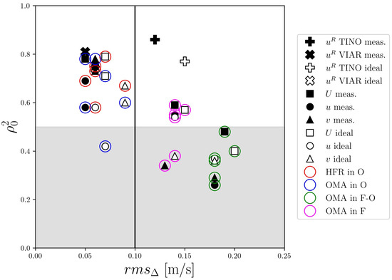
Figure 7.
Statistical results in terms of RMS of the difference and the zero-lag correlation for all variables and configurations. The gray shaded area is for values smaller than 0.5. The ideal radial point for VIAR ( = 0.06 m/s, = 0.74) is below and hidden by the other points nearby.
A similar clustering based on the domains can be observed when looking at the parameter space spanned by the bias and RMS metrics of the difference (Figure 8). The general trend is for negative biases, except for the u component in most configurations (note that the u statistics for measured configurations in the F and F–O domains are below the corresponding ideal ones and not visible in Figure 8 as they have the same values). This is likely to be due to the fact that the radar estimates are averaged and smoothed quantities and generally tend to underestimate the size of the velocity with respect to the drifters. This directly implies that the bias of the speed U is negative, while, for the radial velocities and for the components u and v, the sign depends on the sign of the quantity, which in turn depends on the prevalent velocity direction. We expect a negative bias for mostly positive quantities, while the opposite is true for negative quantities. Given the prevalent northeastward direction of the flow sampled by the drifters (Figure 1), we can expect that only the u component is mostly negative, explaining the positive biases in Figure 8. The configurations in the O sub-domain (red and blue circles) are characterized by small RMS values of , ( m/s), but also by small biases, ( m/s). For the configurations in the full F domain (purple circles), the bias values may exceed m/s, always having medium values ( m/s m/s), while, in the F–O sub-domain (green circles), the bias can exceed . As for the radial velocities, the VIAR system has basically no bias and lower values than the TINO one.
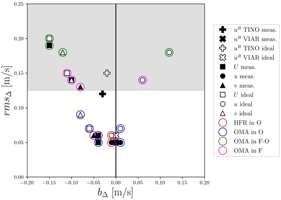
Figure 8.
Statistical results in terms of bias and RMS of the difference for all variables and configurations. The gray shaded area is for values larger than 0.125. Some points (u measured in both F and F–O domains and v measured in the F–O domain) are not visible as they have values equal to the corresponding ideal configurations.
The observed clustering in terms of different domains is likely to be due to at least two factors. First of all, the domain O is sampled by two radars so that all the total velocity statistics are expected to be significantly better. Also, the O domain is less energetic than the northern F–O domain, which can influence both the radial and total velocity statistics. To clarify the effects of the different energetics in the domains, we consider the parameter space spanned by the normalized RMS of the difference , i.e., the , and the zero-lag correlation (Figure 9). If we compare Figure 9 to Figure 7, we see that the clustering is less evident, and there are some interesting similarities and differences. The O total velocities (red and blue) still show the best performances (except for the u component), with ratios lower than and . This confirms the good performance of both the HFR and OMA statistics in regions of adequate coverage. Overall, the worst performance is still found in the F–O domain (green), as in Figure 7, but the difference with the F domain (purple) is less evident. This is because F–O is the most energetic domain, resulting in the very high RMS in Figure 7, which is partially reduced by the normalization. As for the radial velocities, it is interesting to note that the two VIAR and TINO radars now show comparable results, indicating that their differences are primarily due to the different energetics of the sampling domain. Similar results are also shown by the parameter space spanned by the and the bias metrics of the difference , as well as by the parameter space spanned by the bias and the zero-correlation.
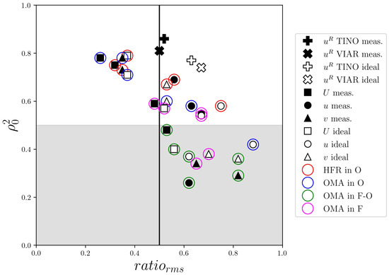
Figure 9.
Statistical results in terms of the ratio between RMS of the difference and the zero-lag correlation for all variables and configurations. The gray shaded area is for values smaller than 0.5.
4. Results for Lagrangian Comparisons
As discussed in Section 2.6.2, drifters were used to validate the HFR OMA total vectors by comparing VD trajectories with RD trajectories. The comparison aims at assessing the reliability of the HFR current fields for estimating the Lagrangian transport in both domains O and F–O and is performed considering first the separation d between the observed and virtual drifter trajectories and then the normalized Skill Score (SS). In both cases, we consider the mean values computed over all the available trajectories during a time window of 1–24 h, after which the drifter trajectories start leaving the domains. The time horizon is relevant for oil spill and SAR applications.
The results for the mean separation are presented together with the mean displacement covered by the drifters (Figure 10a,b) for the O and F–O domains, respectively. The mean displacement in both domains increases almost linearly and reaches 14 km in the O domain and 27 km in F–O in 24 h, indicating that the drifters move under more energetic conditions in the F–O domain, as already discussed in Section 3. The separation d increases much more slowly in domain O and does not exceed 4 km within 24 h, indicating that the HF radar-based trajectories remain quite close to the drifter ones. This is a clear indication that the OMA velocity fields from HF radar perform well in domain O. In the F–O domain, on the other hand, d increases much faster, also with respect to the displacement, reaching 22 km in 24 h. The radar-based trajectories appear to perform acceptably for the first 5 to 10 h when d does not exceed 5 km and is significantly lower than the displacement, but the quality significantly decreases thereafter. This is not surprising given that, in the F–O domain, only one antenna was present.
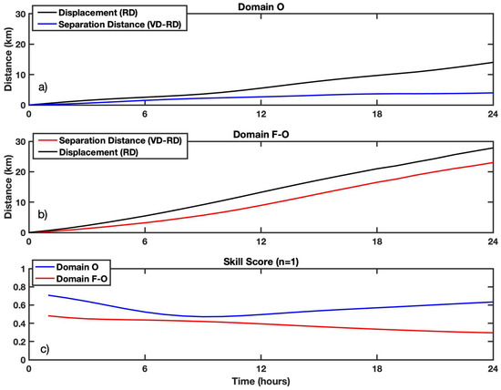
Figure 10.
Comparison between real RD and virtual VD drifter trajectories in (a) Domain O and (b) Domain F–O and (c) the Skill Score in both domains. In gray is the mean absolute distance covered by all the real drifters, and in blue and red the mean separation distance d between drifter- and virtual radar-based trajectories for Domain O and F–O, respectively.
Further assessment of the Lagrangian radar performance occurs using the more complete Skill Score (SS) metric, which provides a normalized and cumulative measure of the distance between the virtual trajectories (VDs) and drifters (RDs) (Figure 10c). The mean SS values are computed at each hour in the considered interval in order to provide a detailed assessment for different time horizons [75].
The SS values for the O domain show an initial decrease from approximately 0.7 to 0.5 during the first 7 h, followed by an increase reaching approximately 0.65 at 24 h. The initial decrease is due to the small-scale variability in the coastal area that is not completely resolved by the radar [75], while the following increase reflects the generally good agreement between the VDs and RDs. The trajectory visual inspection indicates that the VDs move in the same direction as the RDs, even though with slightly reduced velocity, as suggested also by the results in Section 3. Overall, the SS results for O indicate a very good performance of the OMA fields, also compared to other radar and model results [75,81,82,83,84,85].
The results for the F–O domain show a significantly reduced performance, as expected, with decreasing values of SS during the whole time interval, ranging from 0.48 to 0.29 at 24 h. Only during the first 6–7 h do the values remain higher than 0.4, suggesting an acceptable Lagrangian skill. This is confirmed by the visual inspection of the trajectories that indicates that the VDs initially tend to move in the same direction as the RDs, while they significantly separate after a few hours. Given that only information from one antenna is available in the area, the results are actually encouraging, at least for short time scales.
We highlight that the strong dependence of the SS on the time horizon has been investigated by [75], suggesting that short forecast times should be preferred, also in terms of practical applications. In our case, a time horizon of 6 h results in SS = 0.53 for the O domain and 0.43 for the F–O domain, while a time horizon of 24 h yields SS = 0.63 for the O domain and SS = 0.29 for the F–O domain.
5. Summary, Concluding Remarks, and Perspectives
The results presented in this paper show that the performances of the HFR-TirLig network in the NW Med are very satisfactory and compare well with the previous results in the literature, in terms of both the radial velocities and total vector velocities, where the coverage is adequate, i.e., in the area sampled by two radars. In this area, the gap-filled OMA results are equally satisfactory, indicating that the OMA method consistently produces continuous fields without excessive smoothing, which is a possible downside of the gap-filling procedures. The good performance of the OMA fields is also shown by the Lagrangian statistics, characterized by Skill Scores SS = 0.53 at 6 h and 0.63 at 24 h, and an average SS = 0.61 for the first 6 h, indicating that the virtual radar-based trajectories satisfactorily reproduce the observed drifter trajectories. These values are indeed comparable to those reported in the literature, namely SS = 0.32 for the Ibiza HFR network [75], the daily average SS values varying from 0.40 to 0.61 for the Mid-Atlantic HFR network [83], and the mean SS values of 0.4 to 0.7 for the Taiwan Ocean Radar Observing System [82].
In the area covered by one radar only, where the total velocities cannot be computed directly by combining radials, OMA still provides the total velocity estimates. The results are obviously deteriorated with respect to the case of adequate coverage. However, OMA can still provide information regarding the velocity structure and speed, which is useful in several practical applications [69]. Also, in terms of Lagrangian statistics, the results are markedly poorer with respect to the case of two-antenna coverage, especially at 24 h, where SS = 0.29. This is not surprising when also considering that Lagrangian metrics are subject to error cumulation. At the initial times, though, the OMA-based results are characterized by acceptable values, SS = 0.43 at 6 h and an average SS = 0.45 for the first 6 h, suggesting that the information can still be of some value in practical applications.
We notice that the present results mostly apply to the boundary current region, primarily sampled by the drifters that are used for the comparison. While this is the most energetic region and the most relevant to capturing the transport in the Ligurian Sea, it should be underlined that further experiments are necessary to complement the present one to provide a complete assessment of the network, including the interior region.
More generally, the results can be viewed as a first step in the direction of evaluating the OMA performances in the case of one antenna using a comparison with the in situ data in the field. We acknowledge that the application of OMA with one antenna is a very challenging scenario since only one radial component is available, while the rest of the velocity vector information is missing. Indeed, it is possible that the relatively positive results obtained in this case are due to the combination of the dynamics, dominated by the boundary current, and the coverage of the radial component in the direction of the current. For this reason, we think that it is very important that, in future work, the applicability of the OMA method is investigated in a broad range of geographical regions and oceanic environments, including extreme weather or sea conditions, to evaluate its robustness in practical applications.
In summary, the results for HFR networks where the coverage is adequate are positive and support the use of the OMA method to produce near real-time gap-filled velocity products complementing the radially combined products. They are expected to be very useful in several practical applications, especially concerning transport computations. For the extreme case of gap-filling with one antenna only, the present results are encouraging, but substantial further testing is necessary.
Finally, we notice that, in the last few years, the HFR-TirLig network has not only successfully maintained itself despite the difficulties caused by the COVID-19 pandemic lockdown but also significantly expanded and consolidated in terms of the increased number of operational stations and upgraded data transmission and remote-control capabilities. Two new HFR SeaSonde stations operating at 13.5 MHz have been installed in the area between La Spezia and Genova, widening and more than doubling the coverage toward the western Ligurian Sea. Two more phased-array HF radar systems (WERA HF Radar), operating in the 25 MHz band, will be added soon for the higher-resolution monitoring of the currents and waves in front of the Port of Genova. Their measurement area will be partially nested in the larger area already under measurement.
The HFR-TirLig network is part of the Joint European Research Infrastructure of Coastal Observatories (JERICOs, www.jerico-ri.eu, accessed on 30 June 2024), which is promoting HFR best practices development and data and metadata model maintenance and updates. At the national level, the HFR-TirLig network is currently supported by two projects in the framework of the Next Generation EU funding scheme: ITINERIS and RAISE. Under the ITINERIS project, the whole physical infrastructure will be expanded and upgraded, the data processing node will be consolidated, and coordination at the national level for HFR data management will be pursued. The HFR-TirLig network will benefit from ITINERIS activities and vice versa under the umbrella of the EuroGOOS HF Radar Task Team. Under the RAISE project, HFR data will be operationally exploited for improving the nowcasting and forecasting models of the met-ocean conditions in port areas, thus improving the safety and efficiency of port operations. For this task, while classic data assimilation procedures are already underway [86], the next goals for the HFR-TirLig network will be to introduce machine learning methods for improving the automatic quality control and gap-filling of surface current data.
Author Contributions
Conceptualization, M.G.M., A.M., and A.G.; Software, L.C. and Z.K.; Data curation, L.C. and M.B.; Formal analysis, L.C., M.B., Z.K., and A.G.; Investigation, L.C., M.B., and Z.K.; Writing—original draft, L.C., M.B., Z.K., M.G.M., and A.G.; Writing—review and editing, L.C., M.B., Z.K., M.G.M., C.M., A.M., and A.G.; Visualization, Z.K. and M.G.M.; Funding acquisition, C.M., M.G.M., and A.G. All authors have read and agreed to the published version of the manuscript.
Funding
We thank the SICOMAR plus project (EU-funded, PC Interreg VA IFM 2014-2020, Prot. CNR-ISMAR n.6160, 29 August 2018), the SINAPSI project (EU-funded, PC Interreg VA IFM 2014-2020, Prot. CNR-ISMAR n.4632, 26 September 2019), the JERICO-S3 project (EU-funded, H2020, grant number 871153), and the IMPACT project (EU-funded, PC Interreg VA IFM 2014-2020, Prot. ISMAR n. 0002269). We also thank the “3D-pathways (Calypso)” Project (Office of Naval Research—ONR, grant number N00014-18-1-2782). The publication has also been funded by EU—Next Generation EU Mission 4 “Education and Research”—Component 2: “From research to business”—Investment 3.1: “Fund for the realisation of an integrated system of research and innovation infrastructures”—Project IR0000032—ITINERIS—Italian Integrated Environmental Research Infrastructures System—CUP B53C22002150006 and also funded by the European Union—NextGenerationEU and by the Ministry of University and Research (MUR), National Recovery and Resilience Plan (NRRP), Mission 4, Component 2, Investment 1.5, project “RAISE—Robotics and AI for Socio-economic Empowerment” (ECS00000035).U.
Data Availability Statement
The radar data are freely available on the THREDDS Data Server of the European HFR Node (https://thredds.hfrnode.eu, accessed on 30 June 2024) at the “Tyrrhenian_Ligurian_Sea” catalogue (https://thredds.hfrnode.eu:8443/thredds/NRTcurrent/HFR-TirLig/HFR-TirLig_catalog.html, accessed on 30 June 2024) and are distributed via the Copernicus Marine In Situ TAC (http://www.marineinsitu.eu/, accessed on 30 June 2024), EMODnet Physics (https://emodnet.ec.europa.eu/, accessed on 30 June 2024), and SeaDataNet (https://www.seadatanet.org/, accessed on 30 June 2024) data portals. Drifters data are available in the SEANOE catalogue (https://www.seanoe.org/data/00612/72369/, accessed on 30 June 2024).
Acknowledgments
We would like to acknowledge that the author Z.K. is fully supported by the ITINERIS project while L.C., M.C, M.G.M. and A.G. are only partially supported by the same project. M.B. and C.M. are also partially supported by the RAISE Innovation Ecosystem project. Finally, we would like to express our sincere gratitude to the anonymous reviewers for their insightful comments and constructive suggestions, which have significantly improved the quality of this paper.
Conflicts of Interest
The authors declare no conflicts of interest.
Abbreviations
The following abbreviations are used in this manuscript:
| HFR | High Frequency Radar |
| OMA | Open-Boundary Modal Analysis |
| NW Med | Northwestern Mediterranean |
| NC | Northern Current |
| LS | Ligurian Sea |
| TC | Tyrrhenian Current |
| WCC | Western Corsica Current |
| MUSIC | MUltiple SIgnal Classification |
| DOA | Direction Of Arrival |
| CSQ | Raw Cross Spectra Files |
| CSS | Cross Spectra Short Time Files |
| APM | Antenna Pattern Measurement |
| QC | Quality Control |
| CARTHE | Consortium for Advanced Research on Transport of Hydrocarbon in the Environment |
| RMS | Root Mean Square |
| NCLS | Normalized Cumulative Lagrangian Separation |
| SS | Skill Score |
| VD | Virtual Drifter |
| RD | Real (observed) Drifter |
References
- Reyes, E.; Aguiar, E.; Bendoni, M.; Berta, M.; Brandini, C.; Cáceres-Euse, A.; Capodici, F.; Cardin, V.; Cianelli, D.; Ciraolo, G.; et al. Coastal high-frequency radars in the Mediterranean—Part 2: Applications in support of science priorities and societal needs. Ocean Sci. 2022, 18, 797–837. [Google Scholar] [CrossRef]
- Lorente, P.; Aguiar, E.; Bendoni, M.; Berta, M.; Brandini, C.; Cáceres-Euse, A.; Capodici, F.; Cianelli, D.; Ciraolo, G.; Corgnati, L.; et al. Coastal high-frequency radars in the Mediterranean—Part 1: Status of operations and a framework for future development. Ocean. Sci. 2022, 18, 761–795. [Google Scholar] [CrossRef]
- Gurgel, K.W.; Antonischki, G.; Essen, H.H.; Schlick, T. Wellen Radar (WERA): A new ground-wave HF radar for ocean remote sensing. Coast. Eng. 1999, 37, 219–234. [Google Scholar] [CrossRef]
- Rubio, A.; Reyes, E.; Mantovani, C.; Corgnati, L.; Lorente, P.; Solabarrieta, L.; Mader, J.; Fernandez, V.; Pouliquen, S.; Novellino, A.; et al. European High Frequency Radar Network Governance; Project Report; Geomar: Kiel, Germany, 2021. [Google Scholar]
- Mantovani, C.; Corgnati, L.; Horstmann, J.; Rubio, A.; Reyes, E.; Quentin, C.; Cosoli, S.; Asensio, J.L.; Mader, J.; Griffa, A. Best Practices on High Frequency Radar Deployment and Operation for Ocean Current Measurement. Front. Mar. Sci. 2020, 7, 210. [Google Scholar] [CrossRef]
- Roarty, H.; Cook, T.; Hazard, L.; George, D.; Harlan, J.; Cosoli, S.; Wyatt, L.; Alvarez Fanjul, E.; Terrill, E.; Otero, M.; et al. The Global High Frequency Radar Network. Front. Mar. Sci. 2019, 6, 164. [Google Scholar] [CrossRef]
- Rubio, A.; Mader, J.; Corgnati, L.; Mantovani, C.; Griffa, A.; Novellino, A.; Quentin, C.; Wyatt, L.; Schulz-Stellenfleth, J.; Horstmann, J.; et al. HF Radar Activity in European Coastal Seas: Next Steps toward a Pan-European HF Radar Network. Front. Mar. Sci. 2017, 4, 8. [Google Scholar] [CrossRef]
- Wyatt, L.R. A comparison of scatterometer and HF radar wind direction measurements. J. Oper. Oceanogr. 2018, 11, 54–63. [Google Scholar] [CrossRef]
- Wyatt, L.R.; Green, J.J.; Middleditch, A.; Moorhead, M.D.; Howarth, J.; Holt, M.; Keogh, S. Operational Wave, Current, and Wind Measurements with the Pisces HF Radar. IEEE J. Ocean. Eng. 2006, 31, 819–834. [Google Scholar] [CrossRef]
- Wyatt, L.R.; Green, J.J. Developments in Scope and Availability of HF Radar Wave Measurements and Robust Evaluation of Their Accuracy. Remote Sens. 2023, 15, 5536. [Google Scholar] [CrossRef]
- Sciascia, R.; Berta, M.; Carlson, D.F.; Griffa, A.; Panfili, M.; La Mesa, M.; Corgnati, L.; Mantovani, C.; Domenella, E.; Fredj, E.; et al. Linking sardine recruitment in coastal areas to ocean currents using surface drifters and HF radar: A case study in the Gulf of Manfredonia, Adriatic Sea. Ocean. Sci. 2018, 14, 1461–1482. [Google Scholar] [CrossRef]
- Abascal, A.J.; Sanchez, J.; Chiri, H.; Ferrer, M.I.; Cárdenas, M.; Gallego, A.; Castanedo, S.; Medina, R.; Alonso-Martirena, A.; Berx, B.; et al. Operational oil spill trajectory modelling using HF radar currents: A northwest European continental shelf case study. Mar. Pollut. Bull. 2017, 119, 336–350. [Google Scholar] [CrossRef] [PubMed]
- Kokkini, Z.; Zervakis, V.; Mamoutos, I.; Potiris, E.; Frangoulis, C.; Kioroglou, S.; Maderich, V.; Psarra, S. Quantification of the surface mixed-layer lateral transports via the use of a HF radar: Application in the North-East Aegean Sea. Cont. Shelf Res. 2017, 149, 17–31. [Google Scholar] [CrossRef]
- Bellomo, L.; Griffa, A.; Cosoli, S.; Falco, P.; Gerin, R.; Iermano, I.; Kalampokis, A.; Kokkini, Z.; Lana, A.; Magaldi, M.; et al. Toward an integrated HF radar network in the Mediterranean Sea to improve search and rescue and oil spill response: The TOSCA project experience. J. Oper. Oceanogr. 2015, 8, 95–107. [Google Scholar] [CrossRef]
- Kokkini, Z.; Potiris, M.; Kalampokis, A.; Zervakis, V. HF Radar observations of the Dardanelles outflow current in North Eastern Aegean using validated WERA HF radar data. Mediterr. Mar. Sci. 2014, 15, 753–768. [Google Scholar] [CrossRef]
- Lipa; Parikh, H.; Barrick, D.; Roarty, H.; Glenn, S. High-frequency radar observations of the June 2013 US East Coast meteotsunami. Nat. Hazards 2013, 74, 109–122. [Google Scholar] [CrossRef]
- Kohut, J.T.; Glenn, S.M. Improving HF Radar Surface Current Measurements with Measured Antenna Beam Patterns. J. Atmos. Ocean. Technol. 2003, 20, 1303–1316. [Google Scholar] [CrossRef]
- Paduan, J.D.; Kim, K.C.; Cook, M.S.; Chavez, F.P. Calibration and Validation of Direction-Finding High-Frequency Radar Ocean Surface Current Observations. IEEE J. Ocean. Eng. 2006, 31, 862–875. [Google Scholar] [CrossRef]
- Gurgel, K.W.; Barbin, Y.; Schlick, T. Radio Frequency Interference Suppression Techniques in FMCW Modulated HF Radars. In Proceedings of the OCEANS 2007—Europe, Aberdeen, Scotland, 18–21 June 2007; pp. 1–4. [Google Scholar] [CrossRef]
- Kim, S.Y.; Terrill, E.J.; Cornuelle, B.D. Mapping surface currents from HF radar radial velocity measurements using optimal interpolation. J. Geophys. Res. Ocean. 2008, 113, C10. [Google Scholar] [CrossRef]
- Saha, A.K.; Choudhury, S.; Majumder, M. Performance efficiency analysis of water treatment plants by using MCDM and neural network model. MATTER Int. J. Sci. Technol. 2017, 3, 27–35. [Google Scholar] [CrossRef]
- Gauci, A.; Drago, A.; Abela, J. Gap Filling of the CALYPSO HF Radar Sea Surface Current Data through Past Measurements and Satellite Wind Observations. Int. J. Navig. Obs. 2016, 2016, 2–10. [Google Scholar] [CrossRef]
- Mihanović, H.; Cosoli, S.; Vilibić, I.; Ivanković, D.; Dadić, V.; Gačić, M. Surface current patterns in the northern Adriatic extracted from high-frequency radar data using self-organizing map analysis. J. Geophys. Res. Ocean. 2011, 116, C08033. [Google Scholar] [CrossRef]
- Hernández-Carrasco, I.; Solabarrieta, L.; Rubio, A.; Esnaola, G.; Reyes, E.; Orfila, A. Impact of HF radar current gap-filling methodologies on the Lagrangian assessment of coastal dynamics. Ocean. Sci. 2018, 14, 827–847. [Google Scholar] [CrossRef]
- Yaremchuk, M.; Sentchev, A. Mapping radar-derived sea surface currents with a variational method. Cont. Shelf Res. 2009, 29, 1711–1722. [Google Scholar] [CrossRef]
- Yaremchuk, M.; Sentchev, A. A combined EOF/variational approach for mapping radar-derived sea surface currents. Cont. Shelf Res. 2011, 31, 758–768. [Google Scholar] [CrossRef]
- Alvera-Azcárate, A.; Barth, A.; Rixen, M.; Beckers, J. Reconstruction of incomplete oceanographic data sets using empirical orthogonal functions: Application to the Adriatic Sea surface temperature. Ocean. Model. 2005, 9, 325–346. [Google Scholar] [CrossRef]
- Barrick, D.; Fernandez, V.; Ferrer, M.I.; Whelan, C.; Breivik, O. A short-term predictive system for surface currents from a rapidly deployed coastal HF radar network. Ocean. Dyn. 2012, 62, 725–740. [Google Scholar] [CrossRef]
- Kaplan, D.M.; Lekien, F. Spatial interpolation and filtering of surface current data based on open-boundary modal analysis. J. Geophys. Res.-Ocean. 2007, 112, C12007. [Google Scholar] [CrossRef]
- Ohlmann, C.; White, P.; Washburn, L.; Emery, B.; Terrill, E.; Otero, M. Interpretation of Coastal HF Radar–Derived Surface Currents with High-Resolution Drifter Data. J. Atmos. Ocean. Technol. 2007, 24, 666–680. [Google Scholar] [CrossRef]
- Molcard, A.; Poulain, P.M.; Forget, P.; Griffa, A.; Barbin, Y.; Gaggelli, J.; Maistre, J.C.D.; Rixen, M. Comparison between VHF radar observations and data from drifter clusters in the Gulf of La Spezia (Mediterranean Sea). J. Mar. Syst. 2009, 78, S79–S89. [Google Scholar] [CrossRef]
- Corgnati, L.P.; Mantovani, C.; Griffa, A.; Berta, M.; Penna, P.; Celentano, P.; Bellomo, L.; Carlson, D.F.; D’Adamo, R. Implementation and Validation of the ISMAR High-Frequency Coastal Radar Network in the Gulf of Manfredonia (Mediterranean Sea). IEEE J. Ocean. Eng. 2019, 44, 424–445. [Google Scholar] [CrossRef]
- Capodici, F.; Cosoli, S.; Ciraolo, G.; Nasello, C.; Maltese, A.; Poulain, P.M.; Drago, A.; Azzopardi, J.; Gauci, A. Validation of HF radar sea surface currents in the Malta-Sicily Channel. Remote Sens. Environ. 2019, 225, 65–76. [Google Scholar] [CrossRef]
- Millot, C. Circulation in the Western Mediterranean Sea. J. Mar. Syst. 1999, 20, 423–442. [Google Scholar] [CrossRef]
- Astraldi, M.; Bianchi, C.N.; Gasparini, G.P.; Morri, C. Climatic fluctuations, current variability and marine species distribution—A case-study in the Ligurian sea (north-west Mediterranean). Oceanol. Acta 1995, 18, 139–149. [Google Scholar]
- Barth, A.; Alvera-Azcárate, A.; Rixen, M.; Beckers, J.M. Two-way nested model of mesoscale circulation features in the Ligurian Sea. Prog. Oceanogr. 2005, 66, 171–189. [Google Scholar] [CrossRef]
- Sammari, C.; Millot, C.; Prieur, L. Aspects of the seasonal and mesoscale variabilities of the Northern Current in the western Mediterranean Sea inferred from the PROLIG-2 and PROS-6 experiments. Deep. Sea Res. Part I Oceanogr. Res. Pap. 1995, 42, 893–917. [Google Scholar] [CrossRef]
- Sciascia, R.; Magaldi, M.G.; Vetrano, A. Current reversal and associated variability within the Corsica Channel: The 2004 case study. Deep. Sea Res. Part I Oceanogr. Res. Pap. 2019, 144, 39–51. [Google Scholar] [CrossRef]
- Astraldi, M.; Gasparini, G.P.; Manzella, G.M.R.; Hopkins, T.S. Temporal variability of currents in the eastern Ligurian Sea. J. Geophys. Res. Ocean. 1990, 95, 1515–1522. [Google Scholar] [CrossRef]
- Astraldi, M.; Gasparini, G.P. The seasonal characteristics of the circulation in the North Mediterranean Basin and their relationship with the atmospheric-climatic conditions. J. Geophys. Res. 1992, 97, 9531–9540. [Google Scholar] [CrossRef]
- Haza, A.C.; Özgökmen, T.M.; Griffa, A.; Molcard, A.; Poulain, P.M.; Peggion, G. Transport properties in small-scale coastal flows: Relative dispersion from VHF radar measurements in the Gulf of La Spezia. Ocean. Dyn. 2010, 60, 861–882. [Google Scholar] [CrossRef]
- Schroeder, K.; Chiggiato, J.; Haza, A.C.; Griffa, A.; Özgökmen, T.M.; Zanasca, P.; Molcard, A.; Borghini, M.; Poulain, P.M.; Gerin, R.; et al. Targeted Lagrangian sampling of submesoscale dispersion at a coastal frontal zone. Geophys. Res. Lett. 2012, 39, 1–6. [Google Scholar] [CrossRef]
- Ludwig, W.; Dumont, E.; Meybeck, M.; Heussner, S. River discharges of water and nutrients to the Mediterranean and Black Sea: Major drivers for ecosystem changes during past and future decades? Prog. Oceanogr. 2009, 80, 199–217. [Google Scholar] [CrossRef]
- Schmidt, R. Multiple emitter location and signal parameter estimation. IEEE Trans. Antennas Propag. 1986, 34, 276–280. [Google Scholar] [CrossRef]
- Lipa, B.; Nyden, B.; Ullman, D.S.; Terrill, E. SeaSonde Radial Velocities: Derivation and Internal Consistency. IEEE J. Ocean. Eng. 2006, 31, 850–861. [Google Scholar] [CrossRef]
- Abramovich, Y.I.; Johnson, B.A.; Mestre, X. DOA estimation in the small-sample threshold region. In Classical and Modern Direction-of-Arrival Estimation; Elsevier: Amsterdam, The Netherlands, 2009; pp. 219–287. [Google Scholar]
- Cosoli, S.; Mazzoldi, A.; Gačić, M. Validation of Surface Current Measurements in the Northern Adriatic Sea from High-Frequency Radars. J. Atmos. Ocean. Technol. 2010, 25, 908–919. [Google Scholar] [CrossRef]
- Cosoli, S.; Gačić, M.; Mazzoldi, A. Surface current variability and wind influence in the northeastern Adriatic Sea as observed from high-frequency (HF) radar measurements. Cont. Shelf Res. 2012, 33, 1–13. [Google Scholar] [CrossRef]
- Laws, K.; Paduan, J.; Vesecky, J. Estimation and Assessment of Errors Related to Antenna Pattern Distortion in CODAR SeaSonde High-Frequency Radar Ocean Current Measurements. J. Atmos. Ocean. Technol. 2010, 27, 1029–1043. [Google Scholar] [CrossRef]
- Corgnati, L.; Mantovani, C.; Novellino, A.; Rubio, A.; Mader, J. Recommendation Report 2 on Improved Common Procedures for HFR QC Analysis; IFREMER: Brest, France, 2018. [Google Scholar] [CrossRef]
- Kaplan, D.M.; Largier, J.; Botsford, L.W. HF radar observations of surface circulation off Bodega Bay (northern California, USA). J. Geophys. Res. Ocean. 2005, 110, C10020. [Google Scholar] [CrossRef]
- Lipa, B.; Barrick, D. Least-squares methods for the extraction of surface currents from CODAR crossed-loop data: Application at ARSLOE. IEEE J. Ocean. Eng. 1983, 8, 226–253. [Google Scholar] [CrossRef]
- Gurgel, K.W. Shipborne measurement of surface current fields by HF radar. In Proceedings of the OCEANS’94, Brest, France, 13–16 September 1994; Volume 3, pp. 3–23. [Google Scholar]
- Graber, H.C.; Haus, B.K.; Chapman, R.D.; Shay, L.K. HF radar comparisons with moored estimates of current speed and direction: Expected differences and implications. J. Geophys. Res. Ocean. 1997, 102, 18749–18766. [Google Scholar] [CrossRef]
- Lekien, F.; Coulliette, C.; Bank, R.; Marsden, J. Open-boundary modal analysis: Interpolation, extrapolation, and filtering. J. Geophys. Res. Ocean. 2004, 109, C12004. [Google Scholar] [CrossRef]
- Lipphardt, B., Jr.; Kirwan, A., Jr.; Grosch, C.; Lewis, J.; Paduan, J. Blending HF radar and model velocities in Monterey Bay through normal mode analysis. J. Geophys. Res. Ocean. 2000, 105, 3425–3450. [Google Scholar] [CrossRef]
- Chu, P.C.; Ivanov, L.M.; Korzhova, T.P.; Margolina, T.M.; Melnichenko, O.V. Analysis of sparse and noisy ocean current data using flow decomposition. Part I: Theory. J. Atmos. Ocean. Technol. 2003, 20, 478–491. [Google Scholar] [CrossRef]
- Novelli, G.; Guigand, C.M.; Cousin, C.; Ryan, E.H.; Laxague, N.J.M.; Dai, H.; Haus, B.K.; Özgökmen, T.M. A Biodegradable Surface Drifter for Ocean Sampling on a Massive Scale. J. Atmos. Ocean. Technol. 2017, 34, 2509–2532. [Google Scholar] [CrossRef]
- Lumpkin, R.; Özgökmen, T.; Centurioni, L. Advances in the Application of Surface Drifters. Annu. Rev. Mar. Sci. 2017, 9, 59–81. [Google Scholar] [CrossRef] [PubMed]
- Stewart, R.H.; Joy, J.W. HF radio measurements of surface currents. Deep. Sea Res. Oceanogr. Abstr. 1974, 21, 1039–1049. [Google Scholar] [CrossRef]
- Shrira, V.I.; Ivonin, D.V.; Broche, P.; de Maistre, J.C. On remote sensing of vertical shear of ocean surface currents by means of a Single-frequency VHF radar. Geophys. Res. Lett. 2001, 28, 3955–3958. [Google Scholar] [CrossRef]
- Ivonin, D.V.; Broche, P.; Devenon, J.L.; Shrira, V.I. Validation of HF radar probing of the vertical shear of surface currents by acoustic Doppler current profiler measurements. J. Geophys. Res. Ocean. 2004, 109, C04003. [Google Scholar] [CrossRef]
- Guérin, C.A.; Dumas, D.; Molcard, A.; Quentin, C.; Zakardjian, B.; Gramoullé, A.; Berta, M. High-Frequency Radar Measurements with CODAR in the Region of Nice: Improved Calibration and Performance. J. Atmos. Ocean. Technol. 2021, 38, 2003–2016. [Google Scholar] [CrossRef]
- Berta, M.; Bellomo, L.; Magaldi, M.G.; Griffa, A.; Molcard, A.; Marmain, J.; Borghini, M.; Taillandier, V. Estimating Lagrangian transport blending drifters with HF radar data and models: Results from the TOSCA experiment in the Ligurian Current (North Western Mediterranean Sea). Prog. Oceanogr. 2014, 128, 15–29. [Google Scholar] [CrossRef]
- Lorente, P.; Soto-Navarro, J.; Fanjul, E.A.; Piedracoba, S. Accuracy assessment of high frequency radar current measurements in the Strait of Gibraltar. J. Oper. Oceanogr. 2014, 7, 59–73. [Google Scholar] [CrossRef]
- Lorente, P.; Piedracoba, S.; Fanjul, E.A. Validation of high-frequency radar ocean surface current observations in the NW of the Iberian Peninsula. Cont. Shelf Res. 2015, 92, 1–15. [Google Scholar] [CrossRef]
- Lana, A.; Marmain, J.; Fernández, V.; Tintoré, J.; Orfila, A. Wind influence on surface current variability in the Ibiza Channel from HF Radar. Ocean. Dyn. 2016, 66, 483–497. [Google Scholar] [CrossRef]
- Kalampokis, A.; Uttieri, M.; Poulain, P.M.; Zambianchi, E. Validation of HF Radar-Derived Currents in the Gulf of Naples with Lagrangian Data. IEEE Geosci. Remote Sens. Lett. 2016, 13, 1452–1456. [Google Scholar] [CrossRef]
- Vissenaekens, E.; Guizien, K.; Durrieu de Madron, X.; Pairaud, I.; Leredde, Y.; Puig, P.; Bourrin, F. Accuracy of high resolution coastal flow speed simulations during and outside of wind, wave and stratification events (Gulf of Lion, NW Mediterranean). J. Mar. Syst. 2023, 239, 103845. [Google Scholar] [CrossRef]
- Rypina, I.I.; Kirincich, A.R.; Limeburner, R.; Udovydchenko, I.A. Eulerian and Lagrangian Correspondence of High-Frequency Radar and Surface Drifter Data: Effects of Radar Resolution and Flow Components. J. Atmos. Ocean. Technol. 2014, 31, 945–966. [Google Scholar] [CrossRef][Green Version]
- Roarty, H.; Allen, A.A.; Glenn, S.; Kohut, J.T.; Nazzaro, L.; Fredj, E. Evaluation of Environmental Data for Search and Rescue II. In Proceedings of the 2018 OCEANS—MTS/IEEE Kobe Techno-Oceans (OTO), Kobe, Japan, 28–31 May 2018; pp. 1–3. [Google Scholar]
- von Schuckmann, K.; Le Traon, P.-Y.; Smith, N.; Pascual, A.; Djavidnia, S.; Gattuso, J.P.; Grégoire, M.; Nolan, G.; Aaboe, S.; Fanjul, E.Á.; et al. Copernicus Marine Service Ocean State Report, Issue 4. J. Oper. Oceanogr. 2020, 13, S1–S172. [Google Scholar] [CrossRef]
- Liu, Y.; Weisberg, R.H. Evaluation of trajectory modeling in different dynamic regions using normalized cumulative Lagrangian separation. J. Geophys. Res. Ocean. 2011, 116, C9. [Google Scholar] [CrossRef]
- Shen, Y.T.; Lai, J.W.; Leu, L.G.; Lu, Y.C.; Chen, J.M.; Shao, H.J.; Chen, H.W.; Chang, K.T.; Terng, C.T.; Chang, Y.C.; et al. Applications of ocean currents data from high-frequency radars and current profilers to search and rescue missions around Taiwan. J. Oper. Oceanogr. 2019, 12, S126–S136. [Google Scholar] [CrossRef]
- Révelard, A.; Reyes, E.; Mourre, B.; Hernández-Carrasco, I.; Rubio, A.; Lorente, P.; Fernández, C.D.L.; Mader, J.; Álvarez-Fanjul, E.; Tintoré, J. Sensitivity of Skill Score Metric to Validate Lagrangian Simulations in Coastal Areas: Recommendations for Search and Rescue Applications. Front. Mar. Sci. 2021, 8, 630388. [Google Scholar] [CrossRef]
- Chen, A.; Barham, W.; Grooms, I. Comparing Eddy-Permitting Ocean Model Parameterizations via Lagrangian Particle Statistics in a Quasigeostrophic Setting. J. Geophys. Res. Ocean. 2018, 123, 5637–5651. [Google Scholar] [CrossRef]
- Pereiro, D.; Souto, C.; Gago, J. Calibration of a marine floating litter transport model. J. Oper. Oceanogr. 2018, 11, 125–133. [Google Scholar] [CrossRef]
- Tamtare, T.; Dumont, D.; Chavanne, C. Extrapolating Eulerian ocean currents for improving surface drift forecasts. J. Oper. Oceanogr. 2021, 14, 71–85. [Google Scholar] [CrossRef]
- Lipa, B.; Whelan, C.; Rector, B.; Nyden, B. HF Radar Bistatic Measurement of Surface Current Velocities: Drifter Comparisons and Radar Consistency Checks. Remote Sens. 2009, 1, 1190–1211. [Google Scholar] [CrossRef]
- Morey, S.L.; Wienders, N.; Dukhovskoy, D.S.; Bourassa, M.A. Measurement Characteristics of Near-Surface Currents from Ultra-Thin Drifters, Drogued Drifters, and HF Radar. Remote Sens. 2018, 10, 1633. [Google Scholar] [CrossRef]
- Marmain, J.; Molcard, A.; Forget, P.; Barth, A.; Ourmières, Y. Assimilation of HF radar surface currents to optimize forcing in the northwestern Mediterranean Sea. Nonlinear Processes Geophys. 2014, 21, 659–675. [Google Scholar] [CrossRef]
- Fredj, E.; Kohut, J.; Roarty, H.; Lu, J.W. Evaluation of the HF-Radar Network System around Taiwan using Normalized Cumulative Lagrangian Separation. Int. J. Oceanogr. Aquac. 2017, 1, 1–8. [Google Scholar] [CrossRef]
- Roarty, H.; Allen, A.; Glenn, S.; Kohut, J.; Nazzaro, L.; Fredj, E. Evaluation of environmental data for search and rescue. In Proceedings of the OCEANS 2016, Shanghai, China, 10–13 April 2016; pp. 1–3. [Google Scholar] [CrossRef]
- Sotillo, M.G.; Amo-Baladrón, A.; Padorno, E.; García-Ladona, E.; Orfila, A.; Rodríguez-Rubio, P.; Conti, D.; Madrid, J.J.; De los Santos, F.J.; Fanjul, E.A. How is the surface Atlantic water inflow through the Gibraltar Strait forecasted? A lagrangian validation of operational oceanographic services in the Alboran Sea and the Western Mediterranean. Deep. Sea Res. Part II Top. Stud. Oceanogr. 2016, 133, 100–117. [Google Scholar] [CrossRef]
- French-McCay, D.P.; Tajalli-Bakhsh, T.; Jayko, K.; Spaulding, M.L.; Li, Z. Validation of oil spill transport and fate modeling in Arctic ice. Arct. Sci. 2018, 4, 71–97. [Google Scholar] [CrossRef]
- Bendoni, M.; Moore, A.M.; Molcard, A.; Magaldi, M.G.; Fattorini, M.; Brandini, C. 4D-Var data assimilation and observation impact on surface transport of HF-Radar derived surface currents in the North-Western Mediterranean Sea. Ocean. Model. 2023, 184, 102236. [Google Scholar] [CrossRef]


Disclaimer/Publisher’s Note: The statements, opinions and data contained in all publications are solely those of the individual author(s) and contributor(s) and not of MDPI and/or the editor(s). MDPI and/or the editor(s) disclaim responsibility for any injury to people or property resulting from any ideas, methods, instructions or products referred to in the content. |
© 2024 by the authors. Licensee MDPI, Basel, Switzerland. This article is an open access article distributed under the terms and conditions of the Creative Commons Attribution (CC BY) license (https://creativecommons.org/licenses/by/4.0/).