Abstract
Optical satellite data products (e.g., Sentinel-2, PlanetScope, Landsat) require proper validation across diverse ecosystems. This has conventionally been achieved using airborne and more recently unmanned aerial vehicle (UAV) based hyperspectral sensors which constrain operations by both their cost and complexity of use. The MicaSense Altum is an accessible multispectral sensor that integrates a radiometric thermal camera with 5 bands (475 nm–840 nm). In this work we assess the spectral reflectance accuracy of a UAV-mounted MicaSense Altum at 25, 50, 75, and 100 m AGL flight altitudes using the manufacturer provided panel-based reflectance conversion technique for atmospheric correction at the Mer Bleue peatland supersite near Ottawa, Canada. Altum derived spectral reflectance was evaluated through comparison of measurements of six known nominal reflectance calibration panels to in situ spectroradiometer and hyperspectral UAV reflectance products. We found that the Altum sensor saturates in the 475 nm band viewing the 18% reflectance panel, and for all brighter panels for the 475, 560, and 668 nm bands. The Altum was assessed against pre-classified hummock-hollow-lawn microtopographic features using band level pair-wise comparisons and common vegetation indices to investigate the sensor’s viability as a validation tool of PlanetScope Dove 8 band and Sentinel-2A satellite products. We conclude that the use of the Altum needs careful consideration, and its field deployment and reflectance output does not meet the necessary cal/val requirements in the peatland site.
Keywords:
peatland; Mer Bleue; multispectral; calibration; validation; vegetation; hyperspectral; MicaSense; Altum 1. Introduction
Unmanned aerial vehicle (UAV) multispectral sensors have been increasing in popularity given their ability to effectively map and monitor vegetation health, species composition, and overall ecosystem functioning [1,2,3]. The introduction of multispectral remote sensing UAV platforms, due to their affordability, portability, and high temporal and spatial resolution, has substantially lowered the entry costs for collection and processing of multispectral datasets. These data can then be used standalone or to supplement ground- and satellite-based remote sensing [4]. Compared to standard optical (RGB) cameras, multispectral sensors typically contain four to ten bands, including red edge and/or near infrared bands in addition to RGB. This allows for the calculation of standard indices, such as the normalized difference vegetation index (NDVI) for vegetation assessments. The numerous applications and demand for multispectral sensors, in fields such as agriculture, forestry, archaeology and urban planning [5] has resulted in an influx of different multispectral sensors available on the market today. The introduction and rapid adoption of these sensors for data collection [6,7,8,9] demands an independent review of sensor performance to verify the capability of each sensor in practice.
Calibration and validation (cal/val) practices are integral in ensuring accuracy, comparability, standardization, and quality control in multispectral data [10]. Without the proper calibration and validation processes, the reliability and accuracy of multispectral (or hyperspectral) data products can be compromised and result in incorrect or misleading results. Multispectral sensors are usually pre-calibrated at the laboratory by illuminating a reference panel with a calibrated lamp or by using an integrating sphere. Even within the laboratory environment, complex sensor-specific features, such as dark current noise, the vignetting effect, and non-uniformity of the detector, are important considerations to overall sensor performance [11]. After calibration, instruments are subject to their defined limits of operation in the field and often need to be recalibrated over time and use in different environments. Without an accurate radiometric calibration, sensor data are highly susceptible to varying environmental conditions, which consequently influences the measured at-sensor radiance [12]. Even with well-calibrated sensors, in situ targets may be required to improve radiometric accuracy. The most common method is the use of a reference panel, while other widely used methods are downwelling light sensors (DLS) and radiative transfer models [13,14,15,16]. Multispectral (and hyperspectral) imagery thus often requires that the spectral reflectance output of the sensor is compared to “known” ground reflectance spectra. Typically, this is achieved through comparisons to spectroradiometer measurements.
Validation of readily available satellite data reflectance products, such as those from Sentinel-2, the Planet Dove constellation and others (e.g., Landsat), ensures the reliability and accuracy of these satellite sensors for a variety of ecosystems and environments [17,18,19]. This is especially important in areas that are remote and vast, such as northern ecosystems, where satellite data products are the only regularly collected data of the area [2,10]. For this reason, the ease of access of multispectral sensors is particularly appealing to examine, as multispectral sensors provide the potential to improve data collection for up-scaling studies.
The MicaSense Altum (MicaSense, Seattle, WA, USA) is a widely used multi-spectral sensor that integrates a radiometric thermal camera with five spectral bands (475 nm–840 nm). This system uses a calibrated reference panel set up in the field for data acquisition, with an optional UAV mounted DLS. The recommended workflow of the Altum for most UAV image processing software, such as that of Pix4DMapper, performs calibration primarily using a calibrated reference panel (CRP). Higher errors of this radiometric calibration have been reported not only for the Altum, but for other MicaSense sensors, such as the RedEdge series [20,21]. This demands an assessment of the recommended radiometric calibration process and reflectance conversion of the MicaSense Altum workflow, relative to an independent in situ approach using an Empirical Line Method (ELM).
The Micasense Altum sensor has been shown to be a versatile tool in agriculture, its primary use case for monitoring crop health, mapping land use, and assessing water stress. The sensor has been used on UAVs effectively to map land use and land cover (LULC) in smallholder farms [22]. By capturing high-resolution multispectral data and processing this through Google Earth Engine (GEE), the researchers achieved a 91% accuracy in classifying different land cover types. The sensor has also effectively monitored pistachio orchards [23]. The study evaluated various vegetation indices to estimate nut yield and quality under different irrigation treatments. The results showed strong correlations between indices and agronomic parameters. The MicaSense Altum has also been used for precision viticulture, comparing nadir and oblique UAV flights to generate 2D and 3D Crop Water Stress Index maps [24]. This highlights the sensor’s capability to optimize irrigation management and improve water use efficiency in vineyards.
Multispectral sensors, like the Micasense Altum, capture data across a few broad wavelength bands, making them practical for general crop assessments due to their cost-effectiveness and ease of use. Hyperspectral sensors offer higher spectral resolution with many narrow wavelength bands, enabling more detailed and accurate detection of specific crop conditions, such as nutrient deficiencies [25,26] and diseases [27,28]. In this study, a hyperspectral UAV sensor is used to compare and verify the accuracy of the Micasense Altum sensor, ensuring its reliability and exploring how integrating both types of data can improve the precision and effectiveness of ecosystem and agricultural monitoring and management practices.
Our study aims to assess the MicaSense Altum workflow using the provided CRP by utilizing six reference panels of known reflectance to compare spectroradiometer and hyperspectral imagery. The manufacturer recommended workflow is assessed, including the recommended calibration procedure. This was compared to a manual radiometric correction and ELM calibration method. Multispectral data were collected at four altitudes at the Mer Bleue peatland supersite near Ottawa, Canada and examined for both spectral reflectance and spatial accuracy. The Altum was assessed against pre-classified hummock-hollow-lawn microtopographic vegetation features using band level pair-wise comparisons and three common vegetation indices to investigate the sensor’s viability as a validation tool of PlanetScope Dove 8 band and Sentinel-2A satellite ground reflectance products. Our assessment of the usability and performance of the Altum provides protocols that can be applied to similar systems, verifying manufacturer claims of the utility of such UAV sensors for different applications.
2. Materials and Methods
2.1. Study Area
The Mer Bleue Conservation Area (MBCA) is a 35 km2 protected natural area located about 10 km east of Ottawa, ON, Canada (Figure 1A). The area is known for its om-bro-trophic bog, which is a type of acidic, nutrient-poor ecosystem that receives its water and nutrients from precipitation and deposition [29]. The bog is representative of north-ern peatlands and has been extensively studied in terms of its carbon budget and vegetation composition [30,31,32]. Mer Bleue is presently the sole peatland acknowledged as a ‘supersite’ for the Committee on Earth Observation Satellites (CEOS) Land Product Validation (LPV) [33]. These ground reference sites follow established protocols to gather data for validating a minimum of three satellite land products. Additionally, they serve as ongoing, well-supported locations with supporting infrastructure, as well as long-term airborne LiDAR and/or hyperspectral imagery.

Figure 1.
(A) Unmanned aerial vehicle (UAV) photograph of the Mer Bleue Peatland Observatory. (B) UAV photograph of the peatland margin illustrating a beaver pond with open water. (C) Vascular plants in hummocks. (D) Moss vegetation in hollows.
The vegetation in the MBCA is diverse and includes evergreen and deciduous shrubs, such as Chamaedaphne calyculata, Rhododendron groenlandicum, Kalmia angustifolia, and Vaccinium myrtilloides. The bog is also home to patches of sedges, isolated individuals and patches of Picea mariana, Betula populifolia, and Larix laricina, and various species of Sphagnum moss, including S. capillifolium, S. fuscum, and S. magellanicum [34].
The bog itself is characterized by hummock-hollow-lawn microtopographic features, with a mean relief between hummocks (Figure 1C) and hollows (Figure 1D) of less than 30–50 cm. The water table in the bog is spatially and temporally variable, but it is generally below the surface, even in the hollows [35]. Mer Bleue also contains continuously inundated beaver ponds around its margins (Figure 1B), where cattail (Typha angustifolia) and floating Sphagnum can be found.
2.2. MicaSense Altum Data Acquisition
The MicaSense Altum (hereafter referred to as Altum) has five bands between 475 and 842 nm, with a sixth thermal infrared band (8–14 μm) not used in this study. All sensors’ parameters can be found in Table 1. Altum multispectral data were acquired on 23 July 2021, with the Altum mounted on a DJI Matrice 300-RTK (Da-Jiang Innovations, Shenzen, China), hereafter M300, airframe (Figure 2A). The Altum was mounted using a DJI Skyport connection. The automatic triggering option of the overlap mode was used, with DJI Pilot as the flight control software. The Altum can utilize the internal GPS from the downwelling light sensor, but also has the capability to receive position and attitude data from the aircraft, utilized here. The complete recommended acquisition methods (and best practices) were followed from the MicaSense user guide [36]. This includes the automatic calibration panel detection in QR Mode. An image of the calibrated reflectance panel was taken prior to the flights for use in the recommended transfer function for radiance to reflectance for each band. Four flights at differing altitudes above ground level (AGL) were conducted using an 80% image overlap. Closely following the MicaSense recommended flight and camera parameters, the flight parameters for each flight altitude can be found in Table 2.

Table 1.
Summary of Altum characteristics excluding the thermal band.
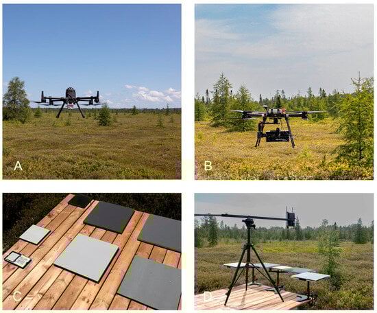
Figure 2.
(A) Altum mounted on the M300. (B) Mjolnir VS-620 hyperspectral sensor mounted on an octocopter with a gimbal for stabilization. (C) Six diffuse reflectance panels (2%, 5%, 10%, 18%, 40%, 50%) and the included MicaSense calibration reflectance panel. (D) HR1024i spectroradiometer taking field measurements of diffuse reflectance panels.
Table 2.
Summary of Altum Flight Parameters.
2.3. Ancillary Data Acquisition (Quality Assurance for Earth Observation Protocol)
In an effort to establish a strategy for common guidelines and protocols for calibration and validation across satellite, UAV, and ground based remote sensing, the European Space Agency (ESA) and, in this context, the Committee on Earth Observation Satellite Land Product Validation sub group (CEOS-LPV) has put focus on the interoperability of remotely sensed data [37]. This is due to the rapidly developed capability of generating Earth observation data outpacing the ability to exploit synergistic interpretations and measurements across the greater remote sensing community. With a focus on traceability, characterized uncertainty budgets and agreed-upon measurement protocols, the Quality Assurance for Earth Observation protocol (QA4EO) provides a framework for achieving interoperability when collecting and processing remote sensing data.
The ancillary data used to complement the Altum data were acquired during a field campaign for a QA4EO project four days prior (19 July 2021). This includes UAV hyperspectral imagery with a HySpex Mjolnir VS-620 (Norsk Elektro Optikk, Oslo, Norway), which consisted of a 120 m altitude flight covering 1.5 hectares resulting in a resampled GSD of 5 cm. Additionally, SPN1 pyranometer (Delta-T Devices, Cambridge, UK) measurements and field and lab-based diffuse panel characterizations were collected on this date. Since this hyperspectral imagery has been previously shown to characterize a series of known reflectance panels meeting the criteria for satellite validation (<3% error) to surface reflectance as described in [38,39], spectral differences between the multispectral, hyperspectral, and satellite vegetation scenes can be attributed to differences in performance between sensors for this ecosystem. The bottom-up calibration/validation approach explored here follows the procedure used in other cal/val exercises at this site [10,17] for satellite product validation from multispectral imagery, as shown in Figure 3, the end goal being to assess multispectral UAV products as a potentially simpler to operate/analyze and cost-effective alternative to UAV hyperspectral data.
Figure 3.
Bottom-up approach to satellite product validation using UAV multispectral imagery.
2.3.1. Mjolnir VS-620 Hyperspectral Imagery
The Mjolnir VS-620 is equipped with two co-aligned push broom hyperspectral imagers, the V-1240 and S-620, which cover the spectral range of 400–2500 nm, although the V-1240 component is most relevant to this study. The system also includes an Inertial Navigation System (INS) (APX-15, Applanix, Richmond Hill, ON, Canada), a data acquisition unit (DAU), a data link to a ground station, and a custom printed circuit board for component control [38,40]. The V-1240 specifications can be found in Table 3. The Mjolnir VS-620 was mounted on a custom octocopter with an H16 XL gimbal (Gremsy, Ho Chi Minh City, Vietnam) for stabilization (Figure 2B). The hyperspectral data were atmospherically corrected using DROACOR (ReSe Applications GmbH, Wil, Switzerland) [41]. The V-1240 had previously been assessed against five reference panels (2–50% reflectance) (Figure 2D).
Table 3.
Summary of Hyspex Mjolnir V-1240 Characteristics.
2.3.2. SPN1 Pyranometer Measurements and Insta360 Hemispherical Photographs
An SPN1 sunshine pyranometer (Delta-T Devices, Cambridge, UK) was used to measure the downwelling global and diffuse broadband irradiance during the QA4EO data collection on 19 July 2021, which had similar blue-sky conditions to the Altum acquisition of the 23rd. The purpose of inclusion of these data was to estimate the impact of operator proximity on the calibration panel reflectance measurement due to blocking of diffuse irradiance by the operator when holding the sensor over the calibration panel. The SPN1 logged measurements over a 5 s integration period every 5 s.
To provide an estimation of the potential impact of this obstructed sky on the reference panel characteristics, hemispherical photos of the unobstructed open sky and that of the operator performing the Altum calibration were collected using a fisheye Insta 360 camera (Arashi Vision Inc., Shenzhen, China).
2.3.3. Spectroradiometer Panel Measurements
A Spectra Vista Corporation (SVC) HR-1024i spectroradiometer (Spectra Vista Corporation, Poughkeepsie, NY, USA), hereafter referred to as HR1024i, was used to characterize the panels in the laboratory and in the field (Figure 2D) using the panel substitution methodology described by [10]. The reflectance panels used in the study consisted of six diffuse reference panels (Labsphere, Inc., North Sutton, NH, USA), with nominal reflectance values of 2% (Spectralon®), 5% (Permaflect®), 10% (Permaflect), 18% (Flexispec®), 40% (Permaflect) and 50% (Spectralon) (Figure 2C). Panel reflectance factors acquired in the laboratory are reported as the biconical reflectance factor BCRF(0°:θi) for a nadir viewing geometry under a particular illumination zenith angle (θi). Panel reflectance factors collected in the field are reported as the hemispherical conical reflectance factor HCRF(0°:θi) for a nadir viewing geometry and a particular solar zenith angle during acquisition. The reader is referred to [10,42] for an in-depth explanation and details of the calculation of BCRF and HCRF. The specifications of the HR1024i can be found in Table 4.
Table 4.
Summary of HR1024i spectroradiometer characteristics.
A high degree of similarity between the laboratory characterization and in situ field measurements is expected if best practices for measurement and calibration are followed [38]. A one nm spacing reflectance factor for the MicaSense panel was provided by the manufacturer. In the absence of additional details on the measurement protocol for this provided spectrum, the full range reflectance properties of the MicaSense reflectance panel were measured in the lab with an Analytical Spectral Devices (ASD) (Malvern Panalytical, Analytik Ltd., Cambridge, UK) Fieldspec-3 spectroradiometer. This reflectance ratio was converted to BCRF(0°:θi) [43].
The output of the HR-1024i (.sig file) was processed using the PySpectra [44] python tool. Using this tool, the data from the HR-1024i was resampled and formatted to be directly compared to the ASD measurements.
2.3.4. Satellite Imagery
To assess the Altum as a satellite validation tool, the multispectral UAV data outputs were also compared to two multispectral satellite products. First, a Sentinel-2 Level-2A atmospherically corrected surface reflectance image of the study area from 23 July 2021 was downloaded from the ESA Copernicus open access hub [45]. The Multispectral Imager (MSI) of Sentinel-2 comprises 13 spectral bands ranging from 10 to 60 m pixel size. The nine bands most relevant (443 nm–865 nm) for the spectral comparison to the Altum (Table 5) were used. The 20 and 60 m bands were resized to 10 m pixels. Second, the PlanetScope SuperDove is a constellation of over 430 U3 form factor satellites with an eight-band frame imager with a butcher block filter [46] (431 nm–885 nm) (Table 5). The PlanetScope SuperDove 8-band surface reflectance product from 23 July 2021 harmonized to Sentinel-2A was downloaded via the PlanetScope ESA archive [47] at a resampled pixel size of 3.0 m.
Table 5.
Summary of satellite data product characteristics. Only the relevant Sentinel-2 bands are listed.
2.4. Analysis
2.4.1. Diffuse Skylight Error Estimation
Based on the recommended MicaSense calibration workflow [36], when holding the Altum and airframe directly above the calibration panel, the operator obstructs a nonzero portion of the diffuse sky irradiance. This results in an alteration of the diffuse illumination that reaches the panel and the sensor and therefore a change in measured reflectance. An important note is that the primary impact is not the obstruction itself but that a similar obstruction is not impacting the downwelling irradiance during the acquisition of the V-1240 hyperspectral imagery. The assumption that this obstruction reduces the diffuse illumination is typically valid for the visible range. However, in the NIR and longer wavelengths, the obstruction is brighter than the sky which results in an increase in illumination relative to the situation in which the obstruction was absent [48]. This obstruction is visualized in Figure 4. The reflectance factor of the operator’s clothing (representing the majority of the obstruction) was determined in the laboratory with 99% and 2% Spectralon panels placed under the fabric to provide the upper and lower bounds.

Figure 4.
MicaSense recommended calibration procedure captured using an Insta360 camera. (a) Visible obstruction of diffuse irradiance during calibration (excluding the holder of the Insta360 at bottom). (b) Unobstructed sky.
The proportion of obstructed sky in steradians was calculated using band thresholds to isolate the obstructing components. These measurements in conjunction with the SPN1 pyranometer data averaged over three hours allows for an estimate of the downwelling and global irradiance measurements, as in Equation (1), and thus the contribution of the blocked hemisphere by the operator will impact the reflectance measurements.
Following Equation (1), represents the global irradiance, with representing direct sunlight, diffuse sunlight and θ zenith angle. One can then use the pyranometer, which measures and , to determine the proportion of the total irradiance resulting from diffuse irradiance. The proportion of the hemisphere obstructed impacts this fraction of the diffuse irradiance by some factor . It then follows that the simplified impact on reflectance (Radjusted) can be estimated by Equation (2):
where is the fraction of hemisphere obstructed by the UAV and holder during the reference panel calibration process (Figure 4a), Rmeasured is the BCRF of Altum panel, and Robstruction is the BCRF of the obstruction.
2.4.2. Reflectance Product of Standard Workflow
The first Altum reflectance product was generated using the recommended workflow and settings of the MicaSense Altum. The output data of each flight consists of a single TIFF for each band, with five total TIFFs per image (excluding the sixth thermal band for analysis), with the total number of images described in Table 2. Using Pix4D Mapper v 4.2.27, which includes the Altum in its camera database, all images can be imported band by band. With this method, the radiometric processing and calibration is largely automated within Pix4D. The radiometric corrections related to the camera settings are completed via the use of EXIF data tagged in each TIFF image, and the calibration step uses the MicaSense calibration panel value for each of the five bands to generate a reflectance product of all images. After this radiometric calibration and processing step, Pix4D Mapper (Pix4D SA, Prilly, Switzerland) generates a reflectance ortho-mosaic through a Structure-from-Motion MultiView Stereo (SfM-MVS) workflow.
2.4.3. Reflectance Product Using Independent Corrections
To assess the standard radiometric calibration workflow, an independent radiometric correction was completed. This was done using the MicaSense GitHub repository [49], which allows for more customization with respect to the processing options for each image. In this instance, metadata was read in manually to compute undistorted radiance using the MicaSense radiometric calibration model described in Equation (3)
which converts the raw pixel values of the image into absolute spectral radiance values in units of W/m2/sr/nm. Here, is the normalized raw pixel value, is the black level value, and are radiometric calibration coefficients, and is the vignette model that corrects for the fall-off of light sensitivity in pixels further from the center of the image. represents the image exposure time, the sensor gain, the pixel row and column, and L the spectral radiance. Many of these model parameters are read from the EXIF metadata, which was carried out using the open source exiftool [50].
An important step in the independent correction is the creation of an aligned capture, or manually adjusting the parameters of the OpenCV homography function to properly align all bands. This required increased processing time and appeared to crop a larger number of pixels from each band than in the standard workflow. Saving these files as radiance GeoTIFF images allowed them to be input into the Pix4D Mapper to be processed as an ortho-mosaic. In this instance, no camera corrections or reflectance calibration are completed in Pix4D; only an ortho-mosaic was created for each of the four altitude datasets.
Once an ortho-mosaic is created, using ENVI v5.6.1 (NV5 Geospatial, Broomfield, CO, USA), an empirical line model (ELM) calibration was performed. This utilized the appropriate non-saturated bands with known diffuse panel HCRF, in this case the 2% and 10% panels, with the assumption of a linear sensor response function to generate reflectance ortho-mosaics for analysis.
2.4.4. Geospatial Offset Calculation
Given that the Mjolnir V-1240 has centimeter level positional accuracy, the offset of each MicaSense Altum dataset was evaluated to assess the range of spatial offsets of the sensor as it relates to altitude. The coordinates from ten points of comparison were extracted per Altum dataset (i.e., 25 m, 50 m, 75 m, and 100 m) to estimate the magnitude of any spatial offsets.
2.4.5. Determination and Comparison of Targets
The comparison of each field panel was conducted following the workflow described in Figure 5. For each altitude collected (i.e., 25 m, 50 m, 75 m, 100 m), the reflectance of the reference panels was assessed within a region of interest (ROI) chosen to definitively include only pixels that were entirely bound within each panel and free of any edge effects that may be influenced by the instrument point-spread function (PSF) or adjacency effects. The reflectance of every panel at every band was assessed to compare to those collected by the resampled spectroradiometer and resampled Mjolnir V-1240. Both the standard MicaSense workflow and the independent radiometric correction and ELM calibration were assessed in their ability to distinguish known reflectance targets.
2.4.6. Comparison of Peatland Vegetation Targets
The workflow used to compare satellite, hyperspectral and the Altum vegetation targets is described in the hummock and hollow comparison in Figure 5. Following appropriate spectral resampling in ENVI to the spectral responses of the Altum bands for the Mjolnir V-1240, a direct band-wise comparison can be made. Similarly, band-wise comparisons can also be made with the Sentinel-2A, and PlanetScope Dove imagery. To compare vegetation targets all four altitude Altum datasets were aligned spatially with the Mjolnir V-1240, ensuring proper pixel comparisons between these two higher resolution products.
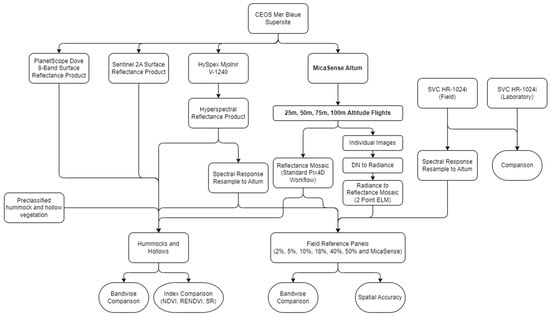
Figure 5.
MicaSense Altum assessment workflow diagram. The field assessment is divided into two sections. Firstly, a comparison is made of panels with known HCRF to both the resampled Mjolnir V-1240 and each Altum flight. The vegetation assessment utilized pre-classified hummock hollow vegetation to compare the two satellite data products to both the Mjolnir V-1240 and Altum output.
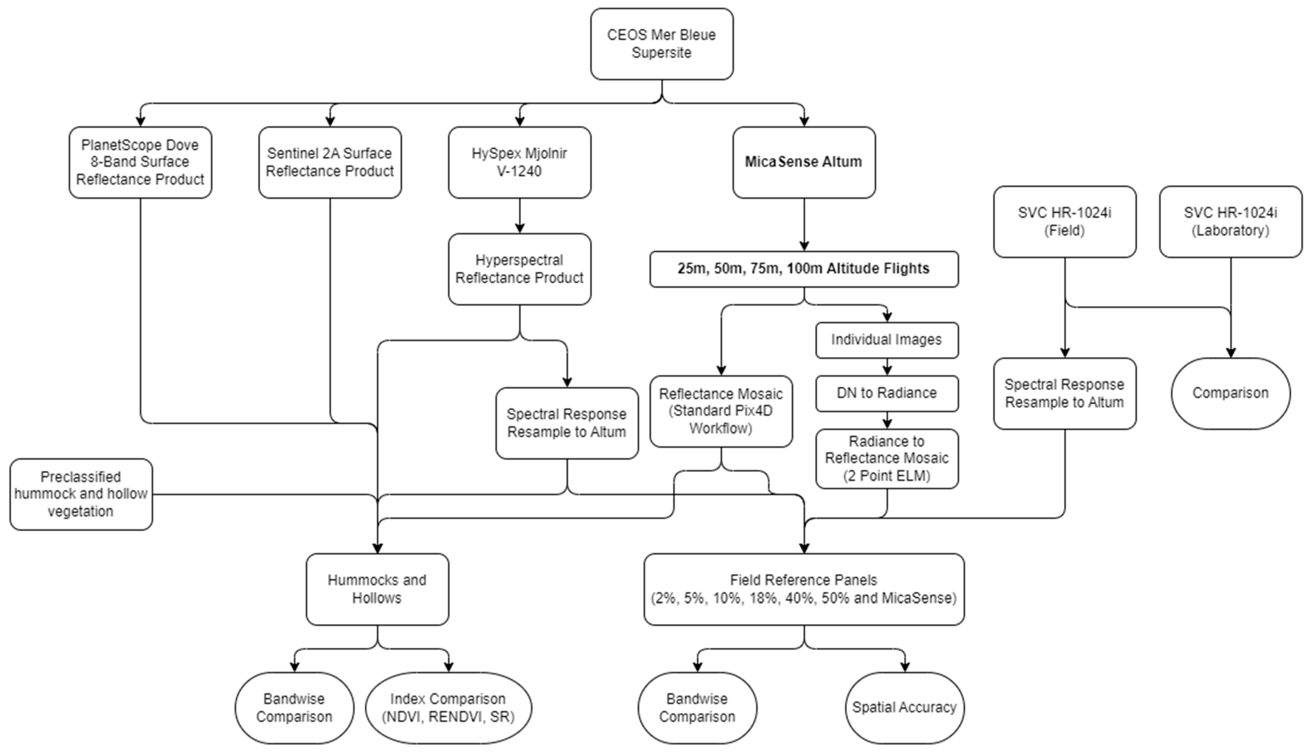
To identify hummock and hollow microtopographic features, a previously developed mask created using hyperspectral data of the entire Mer Bleue peatland [39] was used. This mask identified at fine spatial detail (1 m) the locations of pixels that constitute primarily hummocks, hollows, or other pixels. For the Altum and Mjolnir V-1240 datasets, the area considered for the comparison of this vegetation consisted of the common area to all five datasets (four Altum altitudes and Mjolnir V-1240). This ensures that identical areas are being considered for hummock and hollow comparisons with these imaging systems. For the larger pixels of Sentinel-2A (10 m) and PlanetScope (3 m), there are no pure hummock and hollow pixels for a valid comparison to be conducted in this small area common to the UAV datasets. Therefore, pixels from both the common area of the UAV datasets and the surrounding MBCA were collected for a more complete determination of hummock and hollow targets from the perspective of Sentinel-2 and PlanetScope. This ensured there were an adequate number of pixels from the satellite data for hummocks and hollows to be compared to the UAV collected datasets. Importantly, at the scale of the satellite imagery, the vegetation classes are represented by mixed pixels.
The identification of specific hummock and hollow vegetation types allowed for opportunities to compare band by band for the Altum, Mjolnir V-1240, and satellite products. A calculation of the broadband Normalized Difference Vegetation Index (NDVI) (Equation (4)), the Red-Edge Normalized Difference Vegetation Index (RENDVI) (Equation (5)) and the Simple Ratio Index (SR) (Equation (6)) [51] for hummocks and hollows provided another comparison between the sensors. These three indices can all effectively indicate vegetation, but their differences allow for a more robust comparison of the datasets collected when used together.
For a statistical determination of similarity between spectra and vegetation indices, an ANOVA (Analysis of Variance) test was conducted. This test was used to identify whether there are significant differences between the hummocks and hollows of each dataset both band-wise and for each of the three chosen indices. First, the datasets were verified through an analysis of each distribution and assessed using a Bartlett test for homogeneity of variance. Where there are not the same number of samples and the datasets have unequal variances, Welch’s ANOVA was used to verify that the differences between these datasets is significant, which was then followed up by the appropriate post hoc test. The Games–Howell post hoc test provided pairwise comparisons for all seven datasets both band-wise and for the three indices, such that their agreement can be examined per each dataset pair for seven datasets, i.e., twenty-one comparisons, and associated confidence intervals.
3. Results
3.1. Contribution of Operator Proximity to Reflectance Measurement
The ratio of the diffuse irradiance to total irradiance following Equation (1) when averaged over 3 hours ranged from 15.43 to 15.53% ( = 15.48 = 0.05). The proportion of the hemisphere obstructed by the UAV and operator holding it over the panel was 10.9%. This contributes to a difference between the manufacturer’s MicaSense panel reflectance specifications and the Altum imagery. This contribution to reflectance is shown in Figure 6.

Figure 6.
Comparison between the Rmeasured and Radjusted of the calibration panel reflectance factor based on the proximity of the operator during calibration.
3.2. Spectroradiometer Panel Spectra and Hyperspectral Panel Spectra
Agreement between the laboratory HR1024i panel measurement (dashed) and field HR1024i measurement (solid) in Figure 7 shows that variation in atmospheric and illumination conditions in the field did not have any systematic impact on the reflectance measurement. This close comparison between lab and field measurements has been previously shown [39]. Figure 7 shows the same reference panels with the pixels extracted from the Mjolnir V-1240 resampled to the five bands of the Altum. The Mjolnir V-1240 dataset is within 4% of the field determined HCRF of the panel and is therefore an appropriate UAV baseline measurement against which the performance of the Altum can be compared, i.e., the Altum is expected to characterize the panels similarly to the scatter points in Figure 7.
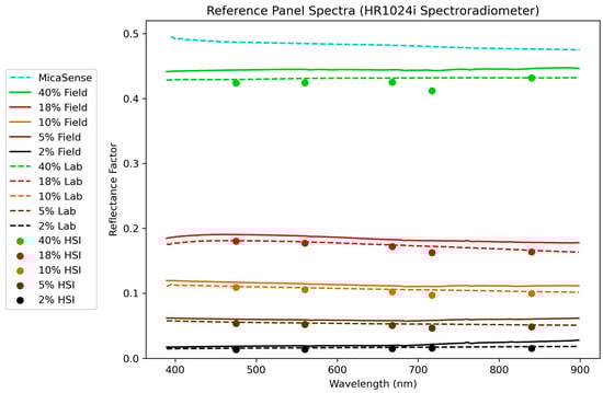
Figure 7.
Diffuse reference panel BCRF measurements in the laboratory with constant illumination conditions and in the field (HCRF) during time of data collection. HR1024i spectroradiometer and laboratory reflectance measurement under constant irradiance (dashed) and HR1024i spectroradiometer and field HCRF measurement (solid) on 19 July 2021. The scattered values are UAV mounted hyperspectral Mjolnir V-1240 reference panel spectra pixel values from 19 July 2021, resampled to the five bands of the Altum.
3.3. Altum Panel Measurements
Utilization of the recommended MicaSense flight parameters for the Altum for each of the four flights resulted in the raw DN shown in Figure 8. In all four flights, the sensor is saturated in several bands for many of the panels, as well as the wooden platform on which the panels are placed in the red band (668 nm). Since the signals are clipped at these points, this results in a total loss of information at higher reflectance for the impacted bands. MicaSense does not recommend adjusting the exposure time and gain from the automatic setting of the sensor, as the camera actively adjusts these settings to ensure the scene is properly exposed. In this case, the camera was unable to identify that the scene was overexposed.
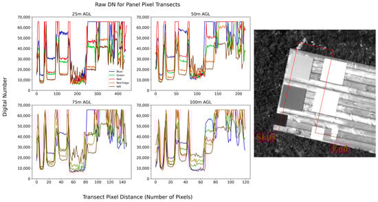
Figure 8.
Saturation of the Altum at the 475 nm, 560 nm, and 668 nm bands. Transect follows path shown on right with each panel labelled on the 25 m AGL graph at the top left.
The recommended MicaSense workflow for the Altum for each of the four flights resulted in a field panel characterization shown in Figure 9a. Given the sensor saturation, the subsequent radiometric calibration is unable to distinguish between the panels where saturation occurred. The blue band saturates at 15% reflectance, whereas the green saturates at 32%. The red band is saturated at 25%. Results of the independent radiometric calibration with an ELM performed with the non-saturated panels (2% and 10%) are shown in Figure 9b. There is close agreement between the two methods in all four altitude datasets, although there is increased variation within panel spectra at increasing altitudes, as would be expected with the potential uncertainty factors of lower resolution and increased transmission distance through the atmosphere at these higher altitudes. This is most evident at the higher altitudes red edge band for the 40%, 50% and MicaSense panels that have a noticeable decrease in reflectance at the two higher altitudes. When compared to the HR1024i BCRF and Mjolnir V-1240 panel reflectance in Figure 7, the Altum is unable to fully characterize the panels.
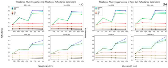
Figure 9.
Reference panel reflectance factor using the recommended MicaSense workflow and independent calibration. (a) Altum panel spectra for all seven reference panels using recommended workflow; (b) Altum panel spectra for all seven reference panels using an independent workflow ELM.
When plotted relative to one another, there is clear deviation between the HR1024i and Altum measurement of the reference panels. Figure 10 shows for both the MicaSense workflow and the independent ELM model that the higher reflectance panels vary in their shorter wavelengths due to the sensor saturation issue and are thus underestimated by the Altum. The Altum also underestimates the highest (50%) reflectance panel in all wavelengths. As expected by the definition of the ELM, the two-point ELM method models the relationship between the low reflectance panels from 2–10% better than the MicaSense method. This comes at the expense of agreement at the higher reflectance targets, most notably the 18% panel, where the MicaSense workflow has closer agreement to the HR1024i measurements.
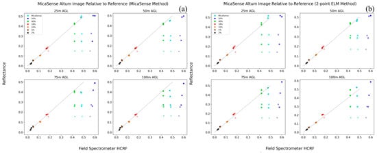
Figure 10.
HR1024i panel HCRF plotted against the MicaSense recommended workflow and independent calibration. Progressively lighter colours indicate shorter wavelengths. Dotted line represents a 1:1 ratio between image and reference reflectance. (a) HR1024i HCRF relative to MicaSense workflow panel measurements; (b) HR1024i HCRF relative to independent ELM calibration panel measurements.
3.4. Altum Spatial Accuracy
To investigate the spatial accuracy of the non-RTK UAV geotags used by the Altum to determine position, it was compared to the Mjolnir V-1240 that utilizes a GNSS navigation system with differential post-processing. Each of the four flights were conducted separately, with computed offsets ranging from 0.07 m to 0.69 m in the x-direction and from −0.22 m to 1.67 m in the y-direction. Figure 11 describes these results with each of the 10 measurements and their combined average offsets included for each altitude flight.
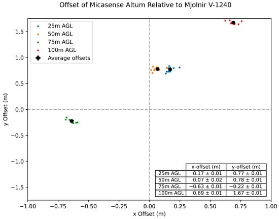
Figure 11.
Spatial offsets identified of the Altum relative to the Mjolnir V-1240.
3.5. Comparison of Vegetation Targets
The mean spectrum of all the pixels in the common overlap area for each dataset is shown in Figure 12. Here, the term “all-pixel comparison” specifically denotes the comparison of all pixels situated within the entire region common to all collected datasets. Detailed information regarding the number and size of hummock and hollow pixels utilized for extraction and analysis is provided in Table 6 for each dataset.
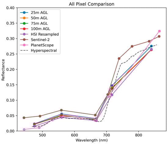
Figure 12.
Comparing all pixels in the common study area to identify differences between sensors independent of the target composition.
Table 6.
Summary of Hummock and Hollow pixel numbers and pixel size for each data source.
A visual interpretation of Figure 13a,b provides several insights. The first is that the four Altum altitudes and resampled Mjolnir V-1240 data do not capture the detailed spectral shapes of the hummocks and hollows as shown by the complete Mjolnir V-1240 data. For example, the wavelength of the red absorption minima is not reflected, nor the inflection point of the near infrared plateau. While the spectral shape of the 8-band PlanetScope Dove and 9 bands of Sentinel-2 approximate the spectra of the UAV data, the inclusion of band 5 on PlanetScope (600–620 nm) captures distinguishing features of the hollows. In contrast, bands 6–8 from Sentinel-2 (740 nm, 783 nm and 842 nm) more closely approximate the shape of the near infrared plateau than any of the other multispectral datasets, which lack bands in that wavelength.
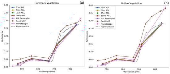
Figure 13.
Comparison of the mean spectra of two complex vegetation targets. (a) Hummock measurements for all Altum altitudes, Mjolnir V-1240 hyperspectral, and two satellite products. (b) Hollow measurements for all Altum altitudes, Mjolnir V-1240 hyperspectral, and two satellite products.
Figure 14 and Figure 15 display the histograms of hummock and hollow data for the UAV datasets. Here, the band-by-band and index comparisons show that, while the distribution may appear Gaussian, a Bartlett test for homogeneity of variance shows that there can be no assumptions of normally distributed data with equal variance (p < 0.01). Thus, statistical analysis is confined to a test that considers unequal sample sizes and variances, such as Welch’s ANOVA. Of note is the difference in the position of the peak in the blue band for both classes between the resampled Mjolnir V-1240 and the Altum datasets (Figure 14). Similarly, the shape of the distribution of RENDVI differs for hummocks and the position of the peak of the distribution differs for the hollows between the resampled Mjolnir V-1240 and the Altum datasets.
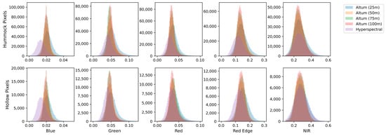
Figure 14.
Histograms of each band (resampled for the Mjolnir V-1240) for hummocks and hollows of the four different altitude Altum datasets and the Mjolnir V-1240 dataset.
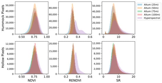
Figure 15.
Histograms of each index investigated for hummocks and hollows of the four different altitude Altum datasets and the Mjolnir V-1240 dataset.
Boxplots were generated to compare each band and index for hummocks and hollows. Band-wise comparisons are described with boxplots in Figure 16, while a comparison of indices is represented in Figure 17. In both cases, the differences between hummock and hollows are more discernable than in the spectra of Figure 13.
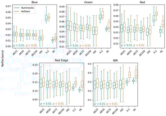
Figure 16.
Boxplots comparing hummock and hollow data per band for seven datasets, the Altum multispectral data collected at four altitudes, the resampled Mjolnir V-1240 hyperspectral, as well as the Sentinel-2A surface reflectance product and PlanetScope Dove 8 band imagery. Abbreviations: Alt25: Altum (25 m), Alt50: Altum (50 m), Alt75: Altum (75 m), Alt100: Altum (100 m), HSI: Hyperspectral, S-2: Sentinel-2A, PS: PlanetScope Dove. The top and bottom of the whiskers in the boxplots represent minimum and maximum values, with the boxes representing the first quartile to the third quartile of values. The horizontal line through each box represents the median value of each dataset.
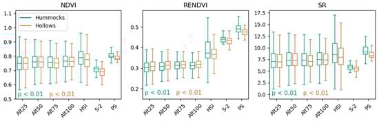
Figure 17.
Boxplots comparing hummock and hollow data for seven datasets at three different indices, the Altum multispectral data collected at four altitudes, the Mjolnir V-1240 hyperspectral, as well as the Sentinel-2A surface reflectance product and PlanetScope Dove 8 band imagery. Abbreviations: Alt25: Altum (25 m), Alt50: Altum (50 m), Alt75: Altum (75 m), Alt100: Altum (100 m), HSI: Hyperspectral, S-2: Sentinel-2A, PS: PlanetScope Dove. The top and bottom of the whiskers in the boxplots represent minimum and maximum values, with the boxes representing the first quartile to the third quartile of values. The horizontal line through each box represents the median value of each dataset.
Each of the altitudes of the Altum datasets are similar for all bands. The visible Altum bands have a consistently higher reflectance than the resampled Mjolnir V-1240. As shown in the spectra of Figure 13 but expanded on here, Sentinel-2A has the highest reflectance relative to all other datasets in the blue, green, red, and near infrared bands, with the red edge being consistent with the UAV datasets. The PlanetScope data are consistent with the UAV data as mentioned previously but has a higher near infrared reflectance relative to the Altum datasets.
In the case of NDVI, the Altum datasets are similar but have lower index values relative to the Mjolnir V-1240 (Figure 17). The NDVI calculated from both Sentinel 2 and PlanetScope, differ from the UAV datasets: Sentinel-2A is ~7% lower and PlanetScope ~5% higher. For RENDVI, the Altum datasets were similar but were 20% lower than from the Mjolnir V-1240 and over 35% lower than Sentinel 2A and 40% lower than PlanetScope. In the case of SR, the results are comparable to NDVI.
Although clear visually from Figure 16 and Figure 17, the results of the Welch’s ANOVA for the seven datasets demonstrated that there are significant differences (p < 0.01) for all datasets for all five bands and three indices. Conducting a Games–Howell post hoc test allows for the direct comparison between each pair of datasets. For seven datasets this constitutes twenty-one comparisons. Figure 18 displays these comparisons for each band, while Figure 19 achieves the same twenty-one comparisons but for the indices.
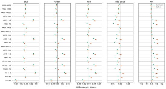
Figure 18.
Multiple comparisons between each of the seven collected datasets for a total of twenty-one comparisons for each of the five bands. The closer to the center line of zero difference in means indicates closer agreement between the pairs. If the confidence interval includes zero, the results are not significantly different from one another. Abbreviations: Alt25: Altum (25 m), Alt50: Altum (50 m), Alt75: Altum (75 m), Alt100: Altum (100 m), HSI: Hyperspectral, S-2: Sentinel-2A, PS: PlanetScope Dove.
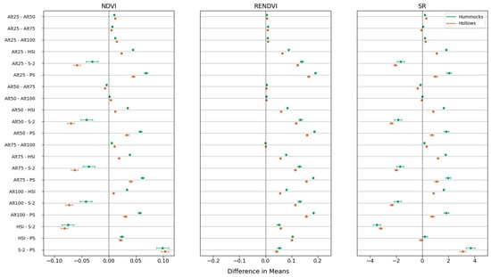
Figure 19.
Multiple comparisons between each of the seven collected datasets for a total of twenty-one comparisons for each of the three indices. The closer to the center line of zero difference in means indicates closer agreement between the pairs. If the confidence interval includes zero, the two compared are not significantly different from one another. Abbreviations: Alt25: Altum (25 m), Alt50: Altum (50 m), Alt75: Altum (75 m), Alt100: Altum (100 m), HSI: Hyperspectral, S-2: Sentinel-2A, PS: PlanetScope Dove.
Figure 18 provides a complement to Figure 16 in the analysis of the difference in means between each dataset. For the blue band, most differences are constrained to 0.01 or less in magnitude of reflectance, with the exception being Sentinel-2A. This is alike for both the green and red bands, where the Sentinel-2A bands have the largest deviations from the other datasets. The red edge band is the most consistent between all datasets, with many comparisons resulting in a non-significantly different result between the two datasets as the difference in mean confidence interval includes zero, particularly for the hollows. In the near infrared, the Altum and Mjolnir V-1240 are both in close agreement for hummocks and hollows, with the two satellite datasets both higher in reflectance.
The comparison of indices in Figure 19 describes pairwise comparisons of the seven datasets. For NDVI, there is close agreement between the different altitude Altum datasets. A difference of 0.008–0.044 can be seen between the Altum and Mjolnir V-1240. Similarly, there are differences of 0.029–0.068 between the Altum-PlanetScope imagery and −0.072–−0.029 between the Altum-Sentinel-2 imagery. In the case of RENDVI, there is greater variability for all comparisons between the Altum and Mjolnir V-1240 and satellite imagery. For SR, results are similar to NDVI.
4. Discussion
Assessing the Altum as a satellite validation tool consisted of investigating the recommended data collection protocol, processing steps, and subsequent outputs. The use of well-characterized UAV hyperspectral imagery in the Mjolnir V-1240 allowed for a comprehensive comparison against the Altum when supplemented with spectroradiometer data as part of the Quality Assurance for Earth Observation (QA4EO) protocol for land product validation. Previous work [17] successfully used hyperspectral imagery to validate Sentinel-2 data, which determined that a high-quality baseline UAV system is capable of validating satellite data. This work took place at the Mer Bleue Conservation Area (MBCA) where the same hummock and hollow complex vegetation targets were assessed. To our knowledge, we present the first attempt to use the Altum as a cost-effective and simpler method to validate satellite data products using a multispectral sensor through the example of characterizing the vegetation of this area.
Evaluating the direct result of operator proximity on reflectance measurements via blocking a portion of the diffuse irradiance is not a novel concept [10]. This is a non-negligible and preventable source of error during collection with MicaSense sensors (Figure 6). The adoption of a racking system or mount that prevents a large obstruction during the calibration procedure would be a relatively inexpensive and effortless process that could be adopted into the standard workflow for the calibration of these sensors. Alternatively, using a larger field reference panel (i.e., 50 cm × 50 cm), the calibration images could be acquired by hovering the drone over the panel. Although perhaps not as relevant for some applications, the fact that the aircraft or DLS GPS is used by default is a potential point of improvement for this sensor. This is especially true with the advent and wide adoption of inexpensive GNSS units capable of providing a PPK or RTK corrected position that would provide centimeter level accuracy, a vast improvement over the large spatial offsets of ~1 m shown here (Figure 11). Such offsets are common to several cameras and RPAS, not geotagging with a corrected position [52]. The Altum has also been shown in a plant phenotyping project [53] to have increased spatial accuracy (cm level) when used in combination with GNSS-Aided Inertial systems allowing for high accuracy Direct Georeferencing (DG), which would eliminate the geospatial offsets seen here.
Close agreement between the HR1024i HCRF in the field and the Mjolnir V-1240 provided a well-defined baseline milestone for the Altum to achieve in characterizing reference panels (Figure 7). Because the MicaSense provided panel could not be characterized by the Altum, and the 18% panel was saturated (Figure 8), this indicates that the automatic exposure time and gain settings may favor increased radiometric resolution at the lower reflectance targets too heavily. One major factor of this inaccuracy is that the calibration panel is imaged at the ground level. This is rectified when using large calibration panels at mission height, but the sensor was saturating, indicating another issue. The intent of the strong recommendation by MicaSense to avoid the use of manual gain and exposure times [54] is that the automatic setting allows for a much larger dynamic range of input when this can be automatically adjusted and is not held fixed by a manual setting. Here, the camera’s automatic adjustment did not perform as needed to prevent the scene from being overexposed in several places. This comes at the expense of not being able to entirely characterize higher reflectance targets in the scene, such as the wooden boardwalk. This is explicitly visualized in Figure 10, with all higher reflectance targets underestimated due to the sensor saturation. In the intended use case of this sensor, which is generally agricultural, this would lead to saturation of soil pixels [55]. As mentioned by MicaSense, manually setting a hard cutoff of exposure time and gain is for advanced users and not recommended as it would force this cutoff where the user desires but is not adjustable between frames. This could be preferred, however, in some cases, where one wants to ensure that the automatic settings do not cause a loss of important data that cannot be collected due to saturation of the sensor. As was in the case in this study, there is also no way to know that the output is saturated using this setting until after collection is complete, which decreases the quality of data over an entire session, or even a campaign of data collection.
In terms of radiometric calibration workflows, the MicaSense environment is accessible and described during each step during the processing from the raw images to radiance and reflectance. In this case, it is easy to unpack and perform one’s own radiometric conversions and subsequently allows for more flexibility in processing. This contrasts with other sensors, such as the MultiSpec 4C, which has reduced opportunity to perform certain steps manually [15].
One large factor that influences the calculation of vegetation indices is the use of broadband indices. With the hyperspectral data capable of measuring the narrowband indices, the use and subsequent comparison of broadband indices for the Altum and satellite products introduces an error related to the differences between what is defined as the red, red edge, and near infrared bands between these different sensors. For example, here the Altum defines red, red edge, and near infrared as 668 nm, 717 nm, and 842 nm respectively. This contrasts to Sentinel-2A, which would use 665.6 nm, 704.1 nm and 864.7 nm, while PlanetScope would use 665.0 nm, 705.0 nm and 864.0 nm. Related to this is the associated full-width half-maximum of each band, which also influences which wavelengths of light are measured and registered. Hyperspectral data can be spectrally resampled and used to calculate a broadband index, allowing it to be compared directly to the Altum or to match satellite data. However, this comparison can introduce other errors and is most useful to see the differences in measurement of the non-resampled bands (Figure 16) and indices (Figure 17), as a test for validation of the satellite product from the Altum sensor “out of the box”.
4.1. Calibration and Assessments of Multispectral Sensor Performance
The MicaSense RedEdge-3, a similar product to the Altum has been characterized in one instance with an integrating sphere and monochromator to offer more effective radiometric calibration procedures and error propagation [21] in the context of monitoring vegetation health. Unfortunately there is a lack of vendor characterization across MicaSense systems, which would lead to reproducible results between individual units, over time, and allow for estimation of uncertainties. With MicaSense sensors, it is up to the user to characterize their own system accurately, which requires specialized equipment that most users do not have access to. With the Altum, we relied on the manufacturer provided “factory” calibration, which can vary as the camera is used in different conditions and over time. Similar to [15] which looked at the RedEdge and MultiSpec 4C, we compared the Altum to spectroradiometer measurements of panels/targets, which in our case had a strong linear relationship for the usable (non-saturated) bands. In other studies, CRPs and/or DLS corrections are used extensively as in [12,20] to provide a radiometric calibration. As in this work, most of these studies use multiple panels and an ELM in comparison to the single MicaSense provided panel to improve outcomes in field validation. The work in [56] used the RedEdge system and compared their more accurate ELM not only to Pix4D’s implementation of the recommended workflow, but also to Metashape, and found the ELM to be more accurate than the manufacturer method when looking at several land covers with a range of intensities, and had no problems with sensor saturation. An agricultural assessment of the Parrot Sequoia and Mini-MCA6 cameras used six calibration panels ranging from 4.5% to 65% reflectance to compare both reflectance as well as NDVI and RENDVI [6], with the 40% and 65% panels saturated in the visible band by the Parrot Sequoia sensor but not by the Mini-MCA6. They found that appropriate radiometric calibration was the most important factor for the effectiveness of the multispectral sensors, especially in the visible (blue, green, and red) bands, although having accurate vegetation index values is not completely dependent on the accuracy of the reflectance. Our Altum digital number saturation in blue, green, and red for our calibration panels was due to the instrument adjusted gain and exposure failing to prevent overexposure, which also occurred for the Sequoia sensor, indicating this occurrence is not exclusive to the Altum. A review of the Parrot Sequoia and MultiSpec 4C sensor calibration methods [57] found no difference between manufacturer-recommended and empirical calibration methods. This study also found digital number saturation in the green band, similar to the Altum, although we found saturation in three bands of our calibration targets. A case using a RedEdge over a water-based environment with an ELM based calibration yielded improved results over the manufacturer recommended calibration [58], noting that atmospheric contributions make greater contributions to the shorter wavelength bands. In a horticultural context, a simplified ELM approach with a Parrot Sequoia and RedEdge was analyzed [59], noting that, in the context of time-series application corrections, irradiance normalization and bidirectional reflectance distribution function (BRDF) corrections also need to be considered, but are not offered in most commercial UAV processing packages. For example, this is an important consideration for future multispectral studies that incorporate phenological shifts. The Parrot Seqouia, when tested in northern latitudes [60], was found to have a difference of up to 10% in peak growing season NDVI depending on radiometric calibration, sun angle, and cloud cover, with radiometric calibration contributing the most to error.
4.2. Satellite Validation of Vegetation Using UAV Multi/Hyper Spectral
High spatial resolution maps like that collected from UAV multi- and hyperspectral systems ease the scale problem between in situ and satellite measurements. In this work we compared hummock and hollow microtopographic features collected by the Altum to the Sentinel-2A reflectance product and PlanetScope Dove 8 band reflectance product. One important consideration with satellite validation using these data in particular is the scale of the UAV data collected, and what this means specifically when identifying these specific vegetation types. In this study, the Altum and hyperspectral data are collected over a relatively small singular area of 0.25 ha and the pixels are not spatially explicit, but are classified based on a previous classification map. Due to the large point spread function and subsequent pixel size of the satellite imagery [61] a comparison of this type, where the hummock and hollow pixels must be identified within a satellite pixel, is limited due to the fact that the study area is heterogeneous with hummocks and hollows at the classification map scale (1 m), meaning there is unavoidable contamination within the satellite pixels from the other class. This is not corrected for in this work and as such the inherent differences as a result of this process in the dataset remain. An alternative method proposed by [62] allows for spatial degradation of fine scale imagery based on the spatial response of a coarser sensor resulting in comparison of spectral properties at the coarsest scale. Additionally, the small number of satellite pixels in the area common to the UAV datasets meant that surrounding pixels (still within the appropriate hummock and hollow classification) contributed. This, in combination with the previous statement on homogeneity, explain at least in part deviations that both the satellite products have from the UAV datasets. In previous validation work at this site that effectively used hyperspectral data to validate Sentinel-2A [17], the main difference is that twenty 5 × 5 Sentinel-2A pixel reference sites were compared to hyperspectral imagery resampled to the same resolution. Since more pixels over a more representative and identical area were being compared, the impact of the point spread functions’ contamination of surrounding pixels of these systems being so large relatively is reduced. In [63], an intercomparison of UAV and satellite reflectance data compared aggregated MicaSense RedEdge and Parrot Seqouia data to Sentinel-2A and Planetscope reflectance products. In that study, there were notable variations in reflectance and index values between spectroradiometer, multispectral, hyperspectral and satellite products. One important result was that the spectral range in satellite data are reduced relative to the UAV collected datasets. This means that data from different sources need to account for spectral sensitivity biases. Comparison between the Parrot Sequoia, Sentinel-2A, and PlanetScope reflectance products was also conducted for onion crops in [64], determining the effect of spatial resolution on analysis in precision agriculture. In this instance there were also clear differences between all platforms. One study comparing the MicaSense RedEdge to Sentinel-2A in agriculture [65] simply conducted an NDVI comparison using fifty random points, which provides a comparison of the same geographic locations but is still impacted by the point spread function of the satellite data introducing influences from neighboring large pixels. It has been well characterized that variation in NDVI determinations from different sensors may be attributed to spatial and radiometric resolutions of the platforms [66]. This study also demonstrates that, because of this increased resolution of UAV multispectral sensors, they overestimate field NDVI value, backed by similar observations using UAV multispectral sensors compared to PlanetScope and Sentinel-2 [67,68,69], which is consistent with the results of this study for Sentinel-2. In a study on vineyards [70], down-sampling of UAV multispectral data was carried out based on pixel clusters of UAV pixel centers within a Sentinel-2A pixel. This study had problems with delineation of inter-row areas contaminating the areas of interest in the satellite pixels, analogous to that of hummocks and hollow classes being closely adjacent.
4.3. Overall Considerations and Future Work
The Altum benefits from high spatial resolution and similar bands to most satellite products. In practice the Altum consistently overestimated reflectance relative to the Mjolnir V-1240. According to Figure 13, the Altum can similarly characterize the hummocks and hollows as does the Mjolnir V-1240. In this case, however, given the performance of the Altum during the calibration assessment, comparisons of raw reflectance that encompass the entirety of systemic errors, such as those resulting from the mentioned sensor settings, must be performed with caution. If any satellite validation is to be achieved with the Altum, it must be carried out not only through reflectance, but through the use of indices that may reduce these factors. However, as shown here with NDVI, SR and especially RENDVI, the differences in index values between the Altum and Mjolnir V-1240 indicate high levels of uncertainty in the Altum index values, making these data unsuitable for validation purposes. When errors in indices such as RENDVI are like that which is shown in Figure 19 on the order of 0.2, sensor output would result in incorrect classification of, for example, crop growth rate status in agricultural settings [71]. Since agriculture is the most common use of multispectral sensors, this warrants careful consideration. This has consequences in the misrepresentation of factors, such as nitrogen supply, crop water stress or overall yield [72]—critical metrics used to assess crop health. Accuracy in reflectance is also essential to monitoring complex vegetation, such as that of peatland bogs explored here. Estimating factors, such as net ecosystem exchange (NEE), from these multispectral sensors requires green, red edge and near-infrared bands, which for a difference of 0.1 red edge expressed here would cause incorrect estimations of NEE [35], and subsequently misrepresent the allogenic and autogenic factors influencing the ecosystem.
The study conducted has some design limitations that can be addressed in future work. Firstly, the study area containing the multispectral imagery was small, and the classification of pixels based on a previous map may not accurately represent finer scale ecosystem variability in such a small area, although it was shown to do so over the entirety of the ecosystem [17]. Expanding the study area and using a more comprehensive classification system could yield more robust and generalizable results. Additionally, the study’s bottom-up approach for satellite validation did not fully account for the inherent differences in pixel sizes, point spread functions, and spectral responses between UAV and satellite data, given that a classification mask was used. Employing a spatial degradation method to align UAV data with satellite sensor characteristics and conducting multi-temporal upscaling analyses would provide a more accurate and reproducible validation framework. This is in line with what is emphasized by the European Space Agency (ESA) and the Committee on Earth Observation Satellite Land Product Validation sub group (CEOS-LPV) [37], as previously mentioned, and a key point of focus for future work using multi- and hyperspectral sensors for satellite validation.
5. Conclusions
This study aimed to evaluate the Altum multispectral sensor’s potential for satellite validation in the context of a northern ombrotrophic bog. By adhering to the bottom-up approach recommended for satellite validation, the Altum’s performance was compared against spectroradiometer and hyperspectral measurements of reference panels and pre-classified complex vegetation.
Our findings indicate that, while the Altum sensor can effectively differentiate between vegetation classes, several limitations hinder its reliability as a long-term validation tool for multispectral satellite products. Notably, issues such as sensor saturation in clear sky environments for the blue band at 15%, green at 32%, and red at 25% reflectance and the resulting inaccuracies in reflectance and spectral vegetation index values emerged as significant challenges.
Positioned within the broader field of remote sensing and satellite validation, this study underscores the critical need for accurate and consistent radiometric calibration in multispectral sensors. Previous research has highlighted the efficacy of high-quality UAV systems in satellite data validation; however, our work demonstrates that the Altum, despite its high spatial resolution and potential, falls short in this regard.
The Altum’s underestimation of reflectance for known reference panels at 18%, 40%, 50% reflectance and the MicaSense provided panel suggest inconsistency in the settings used to operate the Altum “out of the box”. Significant discrepancies in NDVI, SR, and RENDVI indices between the Altum, hyperspectral and satellite products suggest the introduction of uncertainties from the instrument itself. RENDVI particularly was underestimated by the Altum by 20% relative to the hyperspectral, 35% relative to S-2 and 40% relative to PlanetScope. This uncertainty is problematic for applications in agricultural settings and complex ecosystems, like peatlands, where precise measurements are crucial for assessing factors such as crop health, nitrogen supply, crop water stress, overall yield, and net ecosystem exchange (NEE).
Future work should focus on improving the calibration processes for the Altum sensor to mitigate these inaccuracies. The adoption of more robust calibration protocols could enhance the sensor’s reliability. Exploring alternative methods for reducing sensor saturation and better accounting for environmental variables during data collection would position the Altum better as a ready-to-use multispectral platform. Additionally, addressing the limitations of the study primarily in more accurately characterizing the upscaling between in situ, UAV, and satellite measurements is a key point of improvement for future work.
In conclusion, while the Altum multispectral sensor shows promise in vegetation classification, its current limitations in accurate reflectance and spectral vegetation index values restrict its use as a dependable tool for the long-term validation of multispectral satellite products for this study site. Continued advancements in sensor calibration and validation methodologies are essential to harness the full potential of UAV-based multispectral sensors in remote sensing applications.
Author Contributions
Conceptualization, M.K., J.-P.A.-M. and O.L.; methodology, M.K., B.C., R.J.S., D.I. and T.L.; formal analysis, B.C.; investigation, M.K., J.-P.A.-M. and O.L.; writing—original draft preparation, B.C.; writing—review and editing, B.C., M.K., J.-P.A.-M., O.L., D.I. and T.L.; funding acquisition, M.K. and J.-P.A.-M. All authors have read and agreed to the published version of the manuscript.
Funding
This research was funded by the Natural Sciences and Engineering Research Council Canada (NSERC), grant number RGPIN-2022-05288. ESA/SERCO IDEAS-QA4EO Project WP2150.
Data Availability Statement
Data are available upon request.
Acknowledgments
We acknowledge the National Capital Commission for permission to access the research site. We also thank three anonymous reviewers for their comments, which have helped improve the manuscript.
Conflicts of Interest
Author T.L. was employed by the company Norsk Elektro Optikk. The remaining authors declare that the research was conducted in the absence of any commercial or financial relationships that could be construed as a potential conflict of interest.
References
- de Castro, A.I.; Shi, Y.; Maja, J.M.; Peña, J.M. UAVs for Vegetation Monitoring: Overview and Recent Scientific Contributions. Remote Sens. 2021, 13, 2139. [Google Scholar] [CrossRef]
- Fraser, R.H.; Olthof, I.; Lantz, T.C.; Schmitt, C. UAV Photogrammetry for Mapping Vegetation in the Low-Arctic. Arct. Sci. 2016, 2, 79–102. [Google Scholar] [CrossRef]
- Feng, Q.; Liu, J.; Gong, J. UAV Remote Sensing for Urban Vegetation Mapping Using Random Forest and Texture Analysis. Remote Sens. 2015, 7, 1074–1094. [Google Scholar] [CrossRef]
- Yao, H.; Qin, R.; Chen, X. Unmanned Aerial Vehicle for Remote Sensing Applications—A Review. Remote Sens. 2019, 11, 1443. [Google Scholar] [CrossRef]
- King, D.J. Airborne Multispectral Digital Camera and Video Sensors: A Critical Review of System Designs and Applications. Can. J. Remote Sens. 1995, 21, 245–273. [Google Scholar] [CrossRef]
- Deng, L.; Mao, Z.; Li, X.; Hu, Z.; Duan, F.; Yan, Y. UAV-Based Multispectral Remote Sensing for Precision Agriculture: A Comparison between Different Cameras. ISPRS J. Photogramm. Remote Sens. 2018, 146, 124–136. [Google Scholar] [CrossRef]
- Abdollahnejad, A.; Panagiotidis, D. Tree Species Classification and Health Status Assessment for a Mixed Broadleaf-Conifer Forest with UAS Multispectral Imaging. Remote Sens. 2020, 12, 3722. [Google Scholar] [CrossRef]
- Šedina, J.; Housarová, E.; Raeva, P. Using RPAS for the Detection of Archaeological Objects Using Multispectral and Thermal Imaging. Eur. J. Remote Sens. 2019, 52, 182–191. [Google Scholar] [CrossRef]
- Lynch, P.; Blesius, L.; Hines, E. Classification of Urban Area Using Multispectral Indices for Urban Planning. Remote Sens. 2020, 12, 2503. [Google Scholar] [CrossRef]
- Soffer, R.J.; Ifimov, G.; Arroyo-Mora, J.P.; Kalacska, M. Validation of Airborne Hyperspectral Imagery from Laboratory Panel Characterization to Image Quality Assessment: Implications for an Arctic Peatland Surrogate Simulation Site. Can. J. Remote Sens. 2019, 45, 476–508. [Google Scholar] [CrossRef]
- Cao, H.; Gu, X.; Wei, X.; Yu, T.; Zhang, H. Lookup Table Approach for Radiometric Calibration of Miniaturized Multispectral Camera Mounted on an Unmanned Aerial Vehicle. Remote Sens. 2020, 12, 4012. [Google Scholar] [CrossRef]
- Guo, Y.; Senthilnath, J.; Wu, W.; Zhang, X.; Zeng, Z.; Huang, H. Radiometric Calibration for Multispectral Camera of Different Imaging Conditions Mounted on a UAV Platform. Sustainability 2019, 11, 978. [Google Scholar] [CrossRef]
- Aasen, H.; Honkavaara, E.; Lucieer, A.; Zarco-Tejada, P.J. Quantitative Remote Sensing at Ultra-High Resolution with UAV Spectroscopy: A Review of Sensor Technology, Measurement Procedures, and Data Correction Workflows. Remote Sens. 2018, 10, 1091. [Google Scholar] [CrossRef]
- Honkavaara, E.; Saari, H.; Kaivosoja, J.; Pölönen, I.; Hakala, T.; Litkey, P.; Mäkynen, J.; Pesonen, L. Processing and Assessment of Spectrometric, Stereoscopic Imagery Collected Using a Lightweight UAV Spectral Camera for Precision Agriculture. Remote Sens. 2013, 5, 5006–5039. [Google Scholar] [CrossRef]
- Cao, S.; Danielson, B.; Clare, S.; Koenig, S.; Campos-Vargas, C.; Sanchez-Azofeifa, A. Radiometric Calibration Assessments for UAS-Borne Multispectral Cameras: Laboratory and Field Protocols. ISPRS J. Photogramm. Remote Sens. 2019, 149, 132–145. [Google Scholar] [CrossRef]
- Hakala, T.; Markelin, L.; Honkavaara, E.; Scott, B.; Theocharous, T.; Nevalainen, O.; Näsi, R.; Suomalainen, J.; Viljanen, N.; Greenwell, C.; et al. Direct Reflectance Measurements from Drones: Sensor Absolute Radiometric Calibration and System Tests for Forest Reflectance Characterization. Sensors 2018, 18, 1417. [Google Scholar] [CrossRef] [PubMed]
- Arroyo-Mora, J.P.; Kalacska, M.; Soffer, R.; Ifimov, G.; Leblanc, G.; Schaaf, E.S.; Lucanus, O. Evaluation of Phenospectral Dynamics with Sentinel-2A Using a Bottom-up Approach in a Northern Ombrotrophic Peatland. Remote Sens. Environ. 2018, 216, 544–560. [Google Scholar] [CrossRef]
- Loew, A.; Bell, W.; Brocca, L.; Bulgin, C.E.; Burdanowitz, J.; Calbet, X.; Donner, R.V.; Ghent, D.; Gruber, A.; Kaminski, T.; et al. Validation Practices for Satellite-Based Earth Observation Data across Communities. Rev. Geophys. 2017, 55, 779–817. [Google Scholar] [CrossRef]
- Wu, X.; Xiao, Q.; Wen, J.; You, D.; Hueni, A. Advances in Quantitative Remote Sensing Product Validation: Overview and Current Status. Earth-Sci. Rev. 2019, 196, 102875. [Google Scholar] [CrossRef]
- Wang, C. At-Sensor Radiometric Correction of a Multispectral Camera (RedEdge) for sUAS Vegetation Mapping. Sensors 2021, 21, 8224. [Google Scholar] [CrossRef]
- Mamaghani, B.; Salvaggio, C. Multispectral Sensor Calibration and Characterization for sUAS Remote Sensing. Sensors 2019, 19, 4453. [Google Scholar] [CrossRef]
- Gokool, S.; Mahomed, M.; Brewer, K.; Naiken, V.; Clulow, A.; Sibanda, M.; Mabhaudhi, T. Crop Mapping in Smallholder Farms Using Unmanned Aerial Vehicle Imagery and Geospatial Cloud Computing Infrastructure. Heliyon 2024, 10, e26913. [Google Scholar] [CrossRef] [PubMed]
- Martínez-Peña, R.; Vélez, S.; Vacas, R.; Martín, H.; Álvarez, S. Remote Sensing for Sustainable Pistachio Cultivation and Improved Quality Traits Evaluation through Thermal and Non-Thermal UAV Vegetation Indices. Appl. Sci. 2023, 13, 7716. [Google Scholar] [CrossRef]
- Buunk, T.; Vélez, S.; Ariza-Sentís, M.; Valente, J. Comparing Nadir and Oblique Thermal Imagery in UAV-Based 3D Crop Water Stress Index Applications for Precision Viticulture with LiDAR Validation. Sensors 2023, 23, 8625. [Google Scholar] [CrossRef]
- Yu, F.; Bai, J.; Jin, Z.; Guo, Z.; Yang, J.; Chen, C. Combining the Critical Nitrogen Concentration and Machine Learning Algorithms to Estimate Nitrogen Deficiency in Rice from UAV Hyperspectral Data. J. Integr. Agric. 2023, 22, 1216–1229. [Google Scholar] [CrossRef]
- Chancia, R.; Bates, T.; Vanden Heuvel, J.; van Aardt, J. Assessing Grapevine Nutrient Status from Unmanned Aerial System (UAS) Hyperspectral Imagery. Remote Sens. 2021, 13, 4489. [Google Scholar] [CrossRef]
- Zhang, X.; Han, L.; Dong, Y.; Shi, Y.; Huang, W.; Han, L.; González-Moreno, P.; Ma, H.; Ye, H.; Sobeih, T. A Deep Learning-Based Approach for Automated Yellow Rust Disease Detection from High-Resolution Hyperspectral UAV Images. Remote Sens. 2019, 11, 1554. [Google Scholar] [CrossRef]
- Kuswidiyanto, L.W.; Noh, H.-H.; Han, X. Plant Disease Diagnosis Using Deep Learning Based on Aerial Hyperspectral Images: A Review. Remote Sens. 2022, 14, 6031. [Google Scholar] [CrossRef]
- Lafleur, P.M.; Roulet, N.T.; Bubier, J.L.; Frolking, S.; Moore, T.R. Interannual Variability in the Peatland-Atmosphere Carbon Dioxide Exchange at an Ombrotrophic Bog. Glob. Biogeochem. Cycles 2003, 17. [Google Scholar] [CrossRef]
- Strachan, I.B.; Pelletier, L.; Bonneville, M.-C. Inter-Annual Variability in Water Table Depth Controls Net Ecosystem Carbon Dioxide Exchange in a Boreal Bog. Biogeochemistry 2016, 127, 99–111. [Google Scholar] [CrossRef]
- Lafleur, P.M.; Roulet, N.T.; Admiral, S.W. Annual Cycle of CO2 Exchange at a Bog Peatland. J. Geophys. Res. Atmos. 2001, 106, 3071–3081. [Google Scholar] [CrossRef]
- Malhotra, A.; Roulet, N.T.; Wilson, P.; Giroux-Bougard, X.; Harris, L.I. Ecohydrological Feedbacks in Peatlands: An Empirical Test of the Relationship among Vegetation, Microtopography and Water Table. Ecohydrology 2016, 9, 1346–1357. [Google Scholar] [CrossRef]
- CEOS Land Product Validation Subgroup. Available online: https://lpvs.gsfc.nasa.gov/LPV_Supersites/LPVsites.html (accessed on 26 March 2024).
- Eppinga, M.B.; Rietkerk, M.; Borren, W.; Lapshina, E.D.; Bleuten, W.; Wassen, M.J. Regular Surface Patterning of Peatlands: Confronting Theory with Field Data. Ecosystems 2008, 11, 520–536. [Google Scholar] [CrossRef]
- Kalacska, M.; Arroyo-Mora, J.P.; Soffer, R.J.; Roulet, N.T.; Moore, T.R.; Humphreys, E.; Leblanc, G.; Lucanus, O.; Inamdar, D. Estimating Peatland Water Table Depth and Net Ecosystem Exchange: A Comparison between Satellite and Airborne Imagery. Remote Sens. 2018, 10, 687. [Google Scholar] [CrossRef]
- User Guide for MicaSense Sensors. Available online: https://support.micasense.com/hc/en-us/articles/360039671254-User-Guide-for-MicaSense-Sensors (accessed on 12 May 2023).
- Niro, F.; Goryl, P.; Dransfeld, S.; Boccia, V.; Gascon, F.; Adams, J.; Themann, B.; Scifoni, S.; Doxani, G. European Space Agency (ESA) Calibration/Validation Strategy for Optical Land-Imaging Satellites and Pathway towards Interoperability. Remote Sens. 2021, 13, 3003. [Google Scholar] [CrossRef]
- Arroyo-Mora, J.P.; Kalacska, M.; Soffer, R.J.; Lucanus, O. Comparison of Calibration Panels from Field Spectroscopy and UAV Hyperspectral Imagery Acquired Under Diffuse Illumination. In Proceedings of the 2021 IEEE International Geoscience and Remote Sensing Symposium IGARSS, Brussels, Belgium, 11–16 July 2021; pp. 60–63. [Google Scholar]
- Soffer, R.; Arroyo-Mora, J.P.; Kalacska, M.; Ifimov, G.; Leblanc, G. Mer Bleue QA4EO Airborne Hyperspectral Imagery. Borealis, V1. 2022. Available online: https://borealisdata.ca/dataset.xhtml?persistentId=doi:10.5683/SP3/RMGOIW (accessed on 11 May 2023).
- Koirala, P.; Løke, T.; Baarstad, I.; Fridman, A.; Hernandez, J. Real-Time Hyperspectral Image Processing for UAV Applications, Using HySpex Mjolnir-1024. Proc. SPIE 2017, 10198, 64–74. [Google Scholar] [CrossRef]
- ISPRS-Archives-Drone Data Atmospheric Correction Concept for Multi- and Hyperspectral Imagery–The DROACOR Model. Available online: https://isprs-archives.copernicus.org/articles/XLIII-B3-2020/473/2020/ (accessed on 11 May 2023).
- Milton, E.J.; Schaepman, M.E.; Anderson, K.; Kneubühler, M.; Fox, N. Progress in Field Spectroscopy. Remote Sens. Environ. 2009, 113, S92–S109. [Google Scholar] [CrossRef]
- Elmer, K.; Soffer, R.J.; Arroyo-Mora, J.P.; Kalacska, M. ASDToolkit: A Novel MATLAB Processing Toolbox for ASD Field Spectroscopy Data. Data 2020, 5, 96. [Google Scholar] [CrossRef]
- PySpectra/PySpectra at Master · Pmlrsg/PySpectra · GitHub. Available online: https://github.com/pmlrsg/PySpectra/tree/master/PySpectra (accessed on 9 May 2024).
- Open Access Hub. Available online: https://scihub.copernicus.eu/ (accessed on 23 May 2023).
- Understanding PlanetScope Instruments. Available online: https://developers.planet.com/docs/apis/data/sensors/ (accessed on 23 May 2023).
- PlanetScope ESA Archive-Earth Online. Available online: https://earth.esa.int/eogateway/catalog/planetscope-esa-archive (accessed on 23 May 2023).
- Soffer, R. Contamination of Ground Spectral Measurements Due to Operator Proximity. Session WE3.09: Calibration and Validation and standards in support of Spaceborne Imaging Spectroscopy Missions I, Paper 4152. In Proceedings of the IEEE Geoscience And Remote Sensing Society 2014/35th Canadian Symposium for Remote Ssensing, Quebec City, QC, Canada, 13–18 July 2014. [Google Scholar]
- GitHub—Micasense/Imageprocessing: MicaSense RedEdge and Altum Image Processing Tutorials. Available online: https://github.com/micasense/imageprocessing (accessed on 11 May 2024).
- ExifTool by Phil Harvey. Available online: https://exiftool.org/ (accessed on 23 May 2023).
- Xue, J.; Su, B. Significant Remote Sensing Vegetation Indices: A Review of Developments and Applications. J. Sens. 2017, 2017, e1353691. [Google Scholar] [CrossRef]
- Kalacska, M.; Lucanus, O.; Arroyo-Mora, J.P.; Laliberté, É.; Elmer, K.; Leblanc, G.; Groves, A. Accuracy of 3D Landscape Reconstruction without Ground Control Points Using Different UAS Platforms. Drones 2020, 4, 13. [Google Scholar] [CrossRef]
- Hutton, J.J.; Lipa, G.; Baustian, D.; Sulik, J.; Bruce, R.W. high accuracy direct georeferencing of the altum multi-spectral uav camera and its application to high throughput plant phenotyping. Int. Arch. Photogramm. Remote Sens. Spat. Inf. Sci. 2020, XLIII-B1-2020, 451–456. [Google Scholar] [CrossRef]
- Best Practices: Collecting Data with MicaSense Sensors–MicaSense Knowledge Base. Available online: https://support.micasense.com/hc/en-us/articles/224893167-Best-practices-Collecting-Data-with-MicaSense-Sensors (accessed on 15 April 2024).
- Spectral Characteristics Viewer|Landsat Missions. Available online: https://landsat.usgs.gov/spectral-characteristics-viewer (accessed on 15 April 2024).
- Daniels, L.; Eeckhout, E.; Wieme, J.; Dejaegher, Y.; Audenaert, K.; Maes, W.H. Identifying the Optimal Radiometric Calibration Method for UAV-Based Multispectral Imaging. Remote Sens. 2023, 15, 2909. [Google Scholar] [CrossRef]
- Poncet, A.M.; Knappenberger, T.; Brodbeck, C.; Fogle, M.; Shaw, J.N.; Ortiz, B.V. Multispectral UAS Data Accuracy for Different Radiometric Calibration Methods. Remote Sens. 2019, 11, 1917. [Google Scholar] [CrossRef]
- Zarzar, C.; Dash, P.; Dyer, J.; Moorhead, R.; Hathcock, L. Development of a Simplified Radiometric Calibration Framework for Water-Based and Rapid Deployment Unmanned Aerial System (UAS) Operations. Drones 2020, 4, 17. [Google Scholar] [CrossRef]
- Tu, Y.-H.; Phinn, S.; Johansen, K.; Robson, A. Assessing Radiometric Correction Approaches for Multi-Spectral UAS Imagery for Horticultural Applications. Remote Sens. 2018, 10, 1684. [Google Scholar] [CrossRef]
- Assmann, J.J.; Kerby, J.T.; Cunliffe, A.M.; Myers-Smith, I.H. Vegetation Monitoring Using Multispectral Sensors—Best Practices and Lessons Learned from High Latitudes. J. Unmanned Veh. Sys. 2019, 7, 54–75. [Google Scholar] [CrossRef]
- Inamdar, D.; Kalacska, M.; Leblanc, G.; Arroyo-Mora, J.P. Characterizing and Mitigating Sensor Generated Spatial Correlations in Airborne Hyperspectral Imaging Data. Remote Sens. 2020, 12, 641. [Google Scholar] [CrossRef]
- Inamdar, D.; Kalacska, M.; Darko, P.O.; Arroyo-Mora, J.P.; Leblanc, G. Spatial Response Resampling (SR2): Accounting for the Spatial Point Spread Function in Hyperspectral Image Resampling. Methods X 2023, 10, 101998. [Google Scholar] [CrossRef] [PubMed]
- Slade, G.; Fawcett, D.; Cunliffe, A.M.; Brazier, R.E.; Nyaupane, K.; Mauritz, M.; Vargas, S.; Anderson, K. Optical Reflectance across Spatial Scales—An Intercomparison of Transect-Based Hyperspectral, Drone, and Satellite Reflectance Data for Dry Season Rangeland. Drone Syst. Appl. 2023, 11, 1–20. [Google Scholar] [CrossRef]
- Messina, G.; Peña, J.M.; Vizzari, M.; Modica, G. A Comparison of UAV and Satellites Multispectral Imagery in Monitoring Onion Crop. An Application in the ‘Cipolla Rossa Di Tropea’ (Italy). Remote Sens. 2020, 12, 3424. [Google Scholar] [CrossRef]
- Jain, K.; Pandey, A. Calibration of Satellite Imagery with Multispectral UAV Imagery. J. Indian Soc. Remote Sens. 2021, 49, 479–490. [Google Scholar] [CrossRef]
- Ihuoma, S.O.; Madramootoo, C.A.; Kalacska, M. Integration of Satellite Imagery and in Situ Soil Moisture Data for Estimating Irrigation Water Requirements. Int. J. Appl. Earth Obs. Geoinf. 2021, 102, 102396. [Google Scholar] [CrossRef]
- Gago, J.; Douthe, C.; Coopman, R.E.; Gallego, P.P.; Ribas-Carbo, M.; Flexas, J.; Escalona, J.; Medrano, H. UAVs Challenge to Assess Water Stress for Sustainable Agriculture. Agric. Water Manag. 2015, 153, 9–19. [Google Scholar] [CrossRef]
- Zarco-Tejada, P.J.; González-Dugo, V.; Berni, J.A.J. Fluorescence, Temperature and Narrow-Band Indices Acquired from a UAV Platform for Water Stress Detection Using a Micro-Hyperspectral Imager and a Thermal Camera. Remote Sens. Environ. 2012, 117, 322–337. [Google Scholar] [CrossRef]
- Turner, D.; Lucieer, A.; Watson, C. An Automated Technique for Generating Georectified Mosaics from Ultra-High Resolution Unmanned Aerial Vehicle (UAV) Imagery, Based on Structure from Motion (SfM) Point Clouds. Remote Sens. 2012, 4, 1392–1410. [Google Scholar] [CrossRef]
- Khaliq, A.; Comba, L.; Biglia, A.; Ricauda Aimonino, D.; Chiaberge, M.; Gay, P. Comparison of Satellite and UAV-Based Multispectral Imagery for Vineyard Variability Assessment. Remote Sens. 2019, 11, 436. [Google Scholar] [CrossRef]
- Burns, B.W.; Green, V.S.; Hashem, A.A.; Massey, J.H.; Shew, A.M.; Adviento-Borbe, M.A.A.; Milad, M. Determining Nitrogen Deficiencies for Maize Using Various Remote Sensing Indices. Precis. Agric. 2022, 23, 791–811. [Google Scholar] [CrossRef]
- Olson, D.; Anderson, J. Review on Unmanned Aerial Vehicles, Remote Sensors, Imagery Processing, and Their Applications in Agriculture. Agron. J. 2021, 113, 971–992. [Google Scholar] [CrossRef]

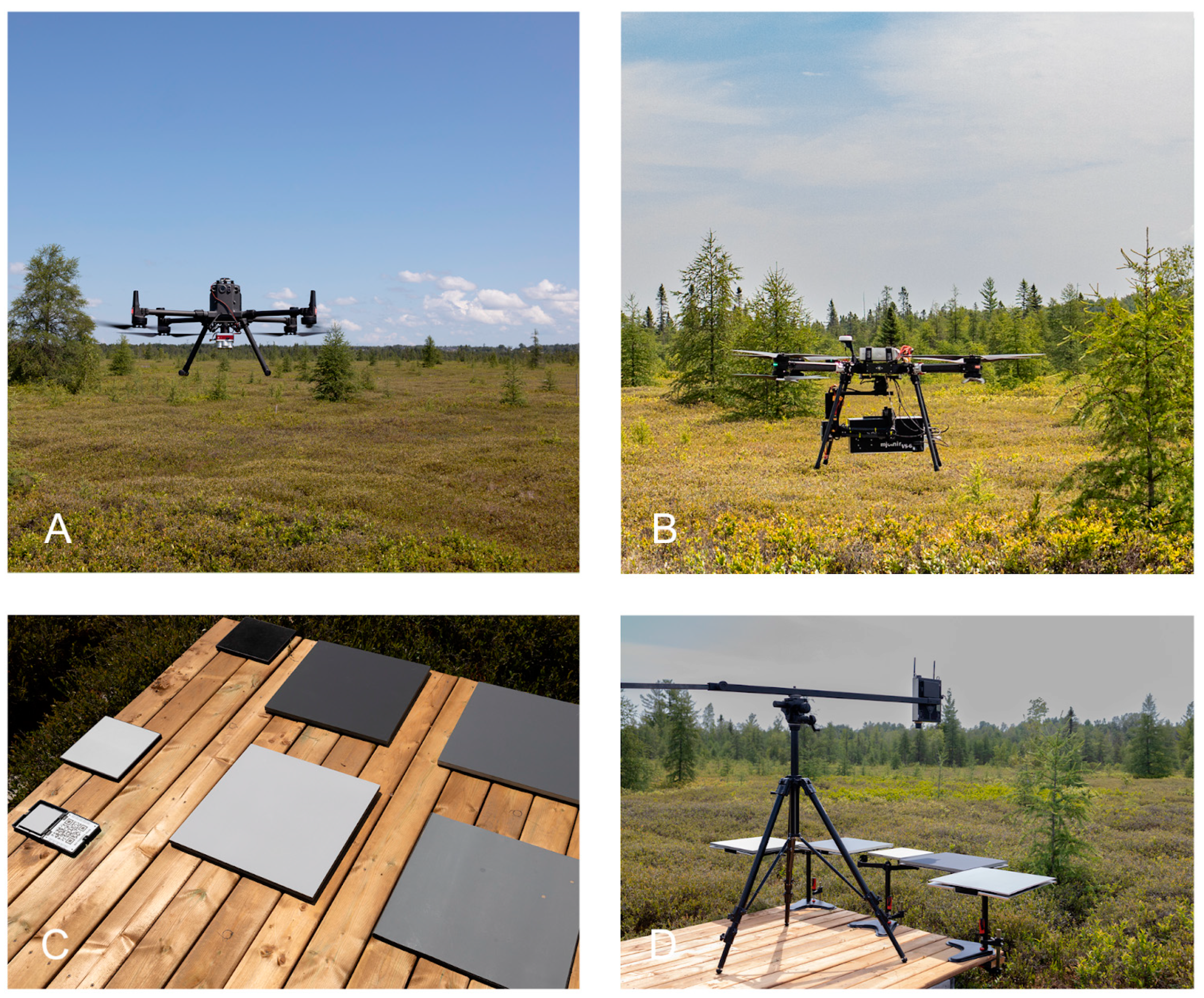

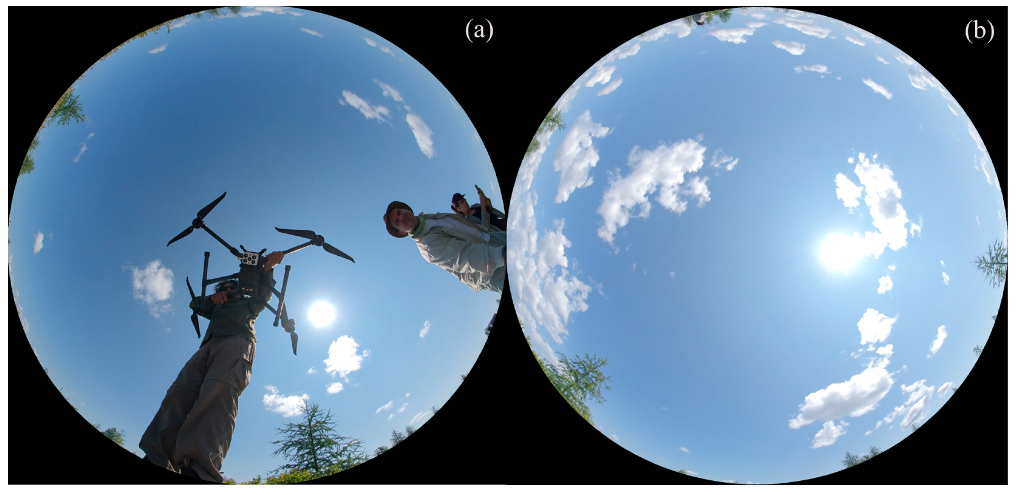
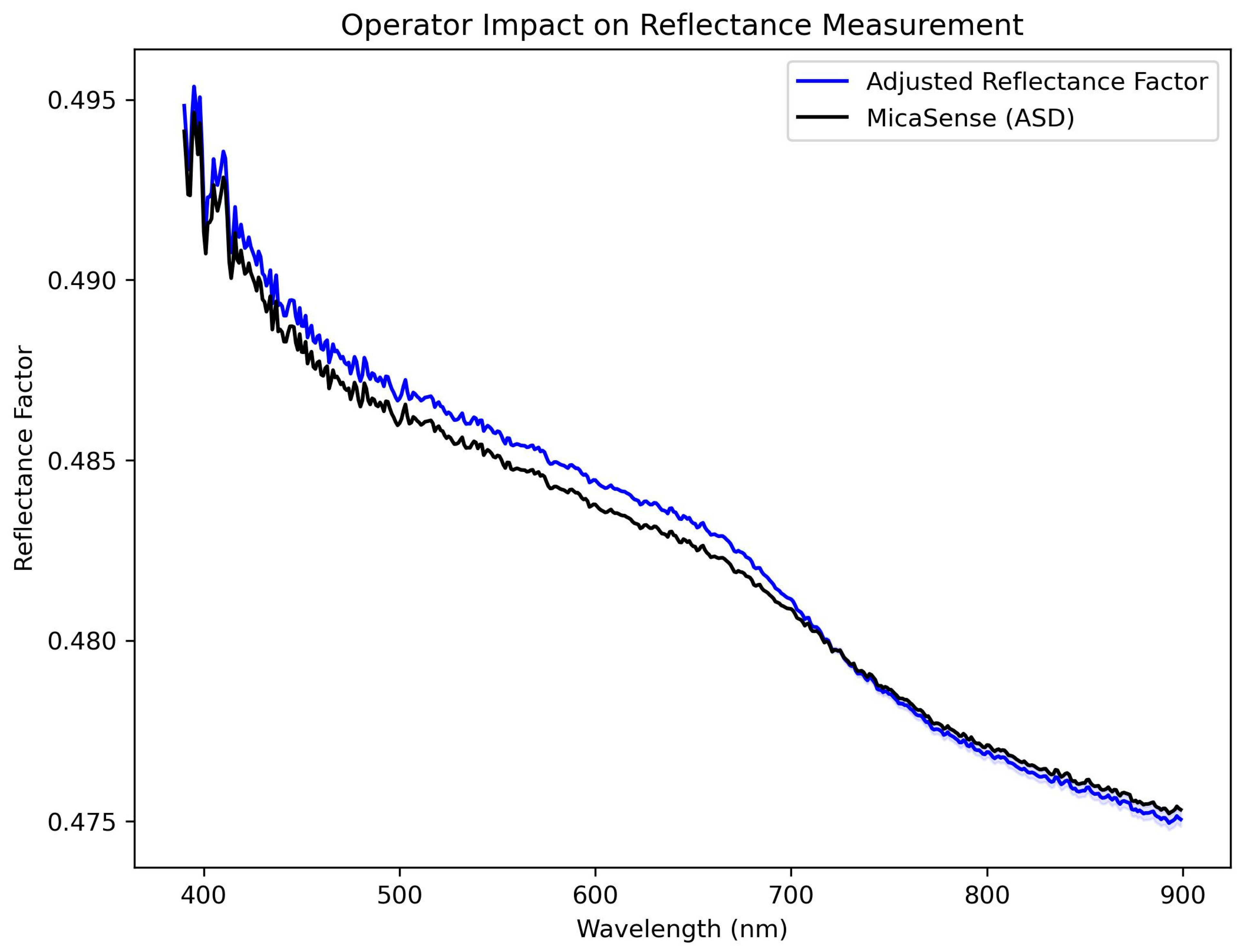
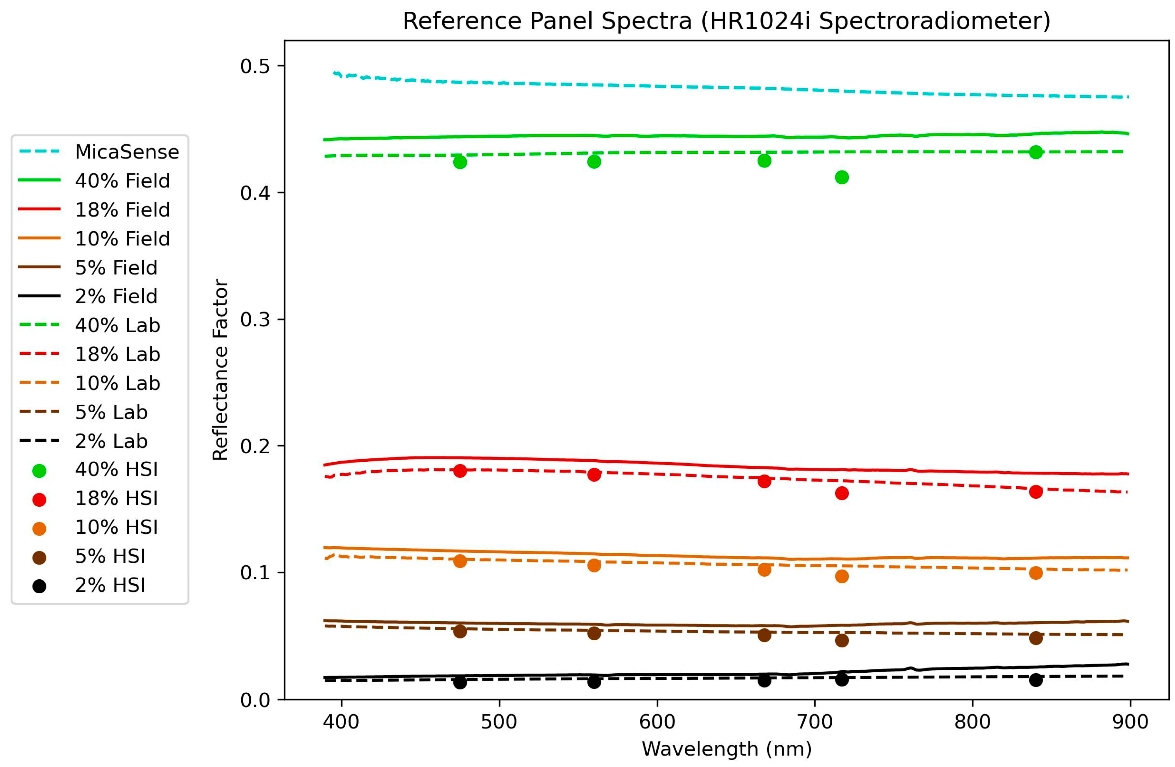
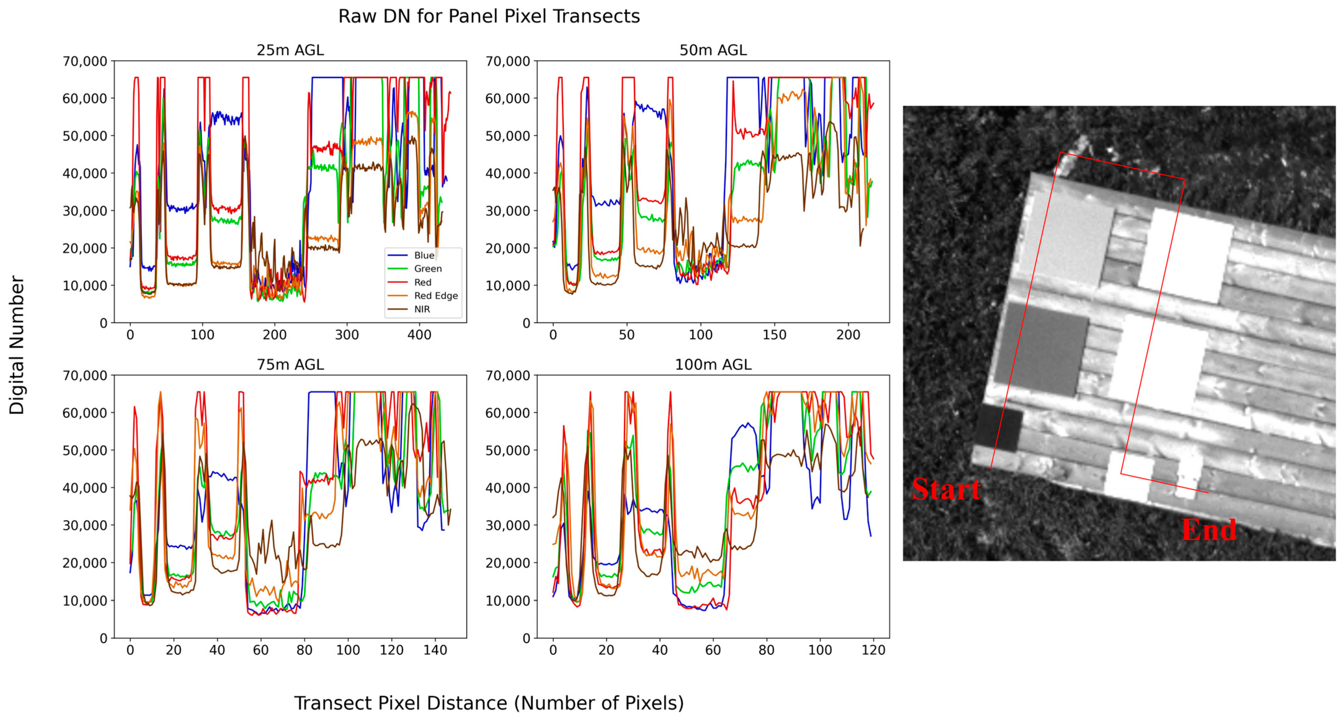
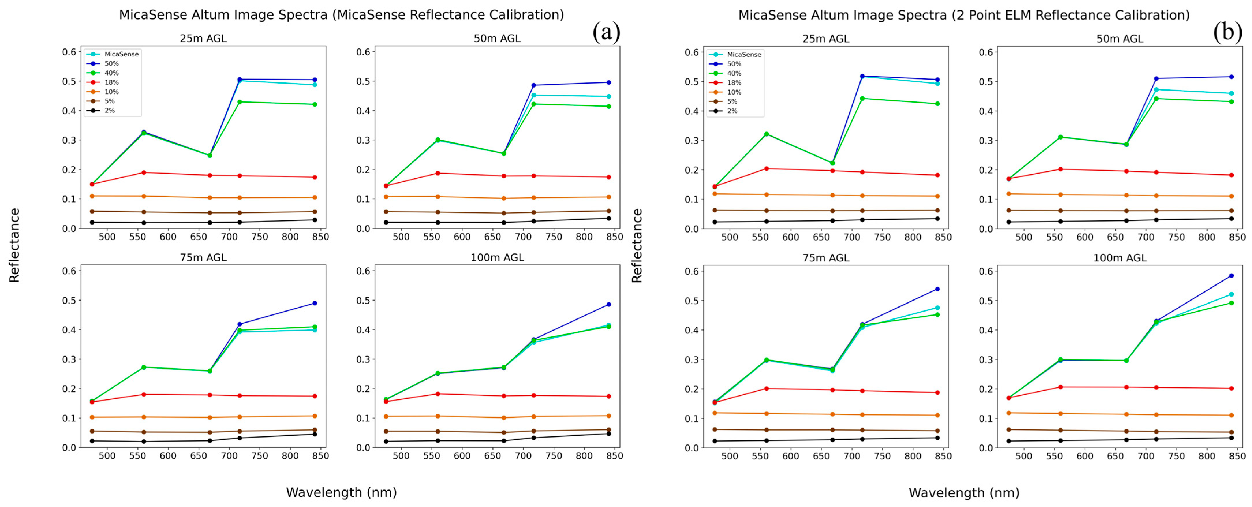
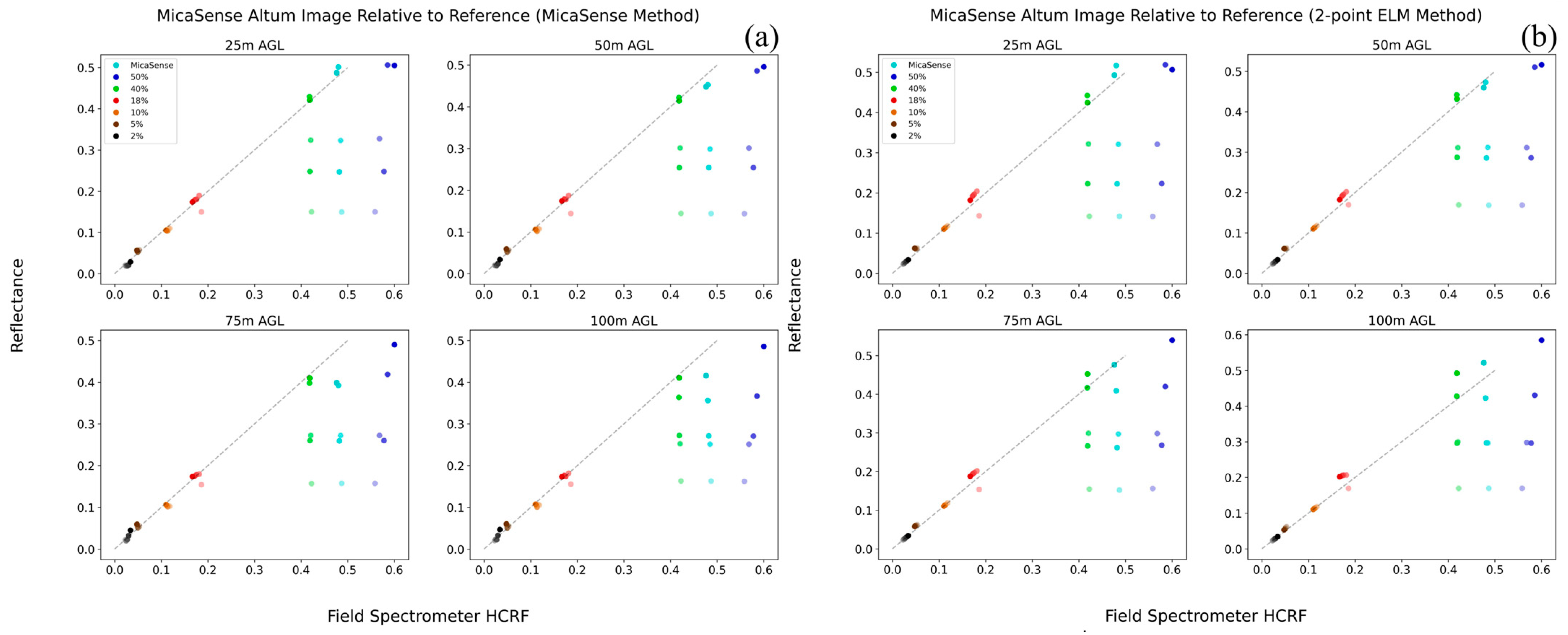
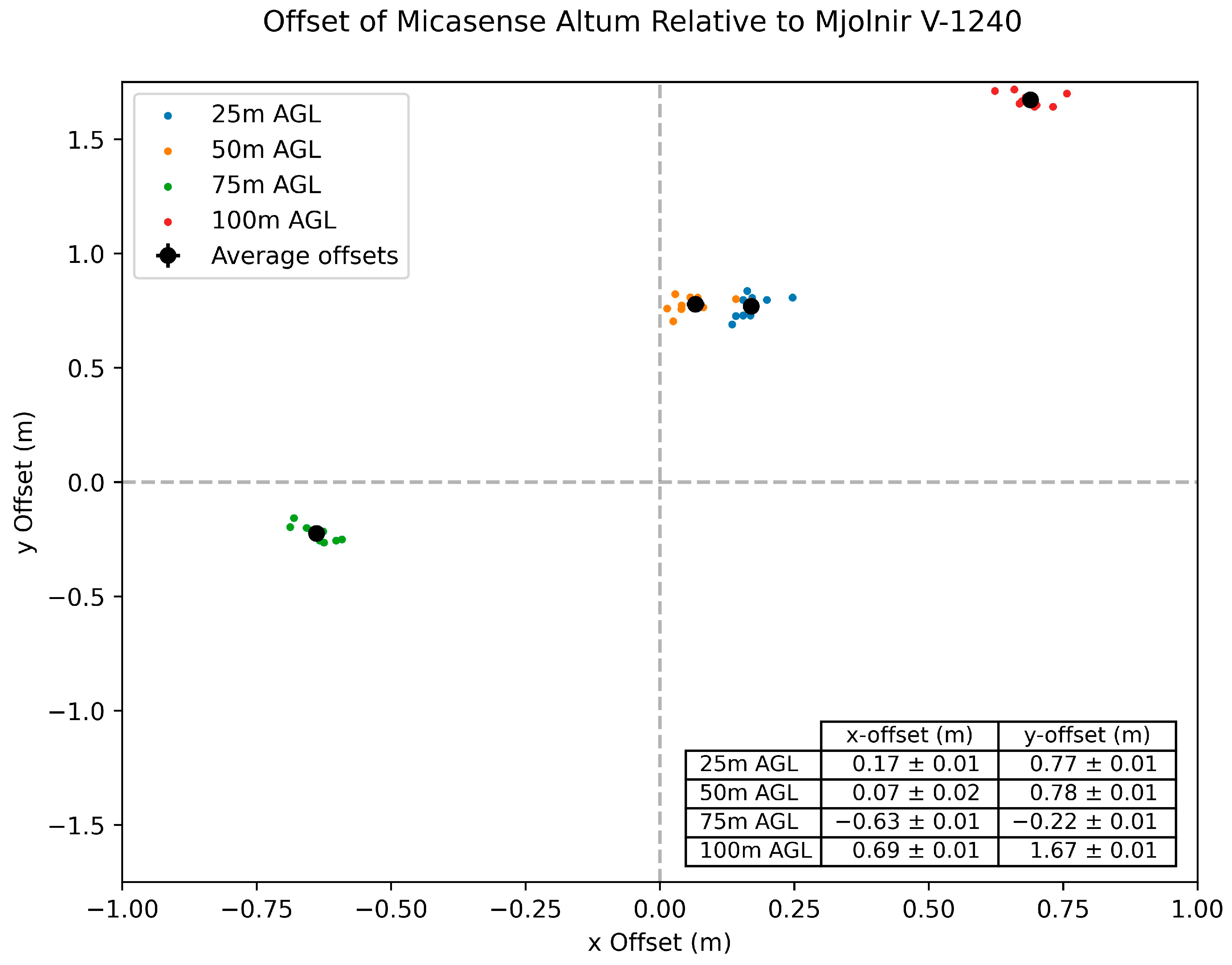
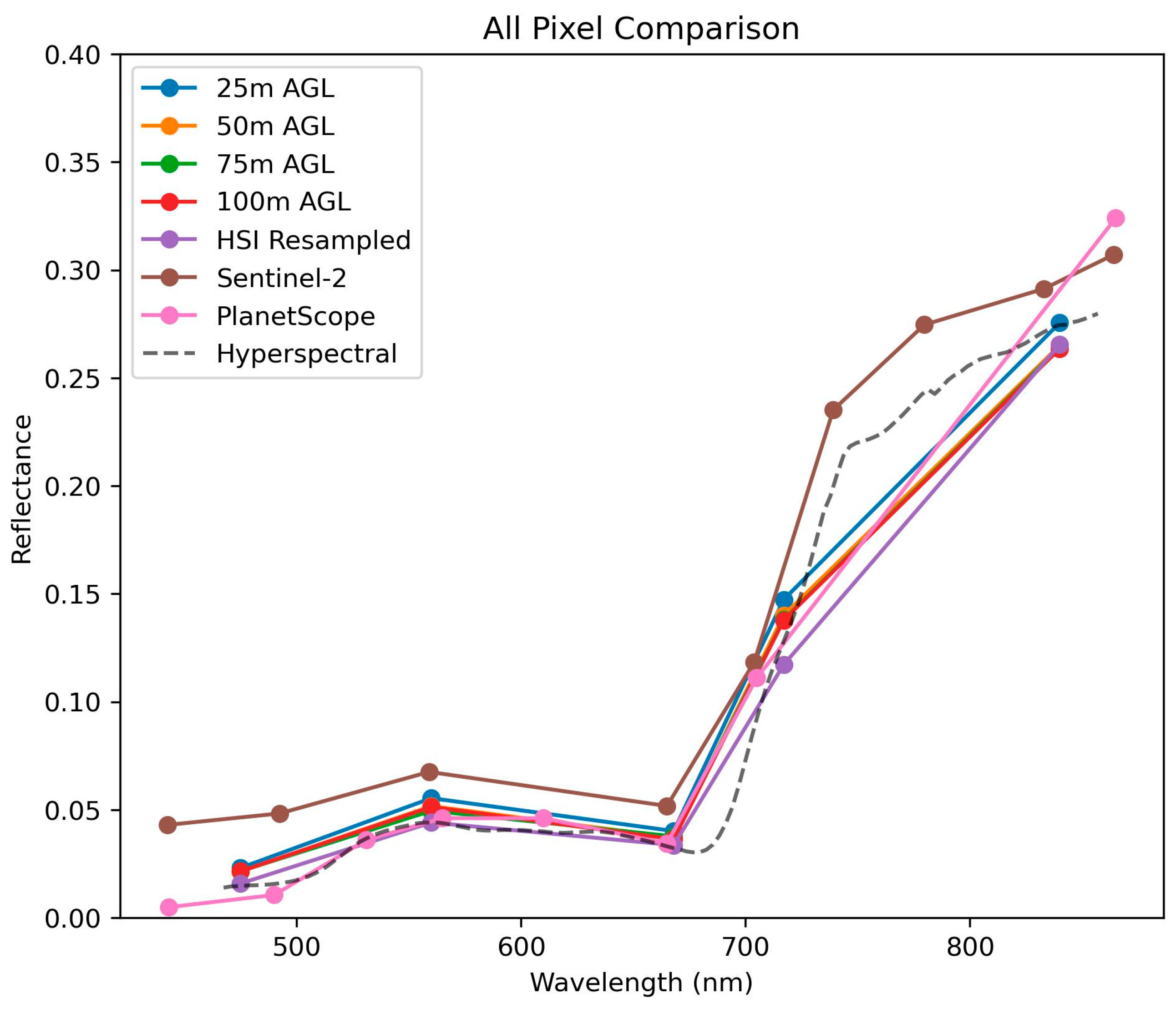
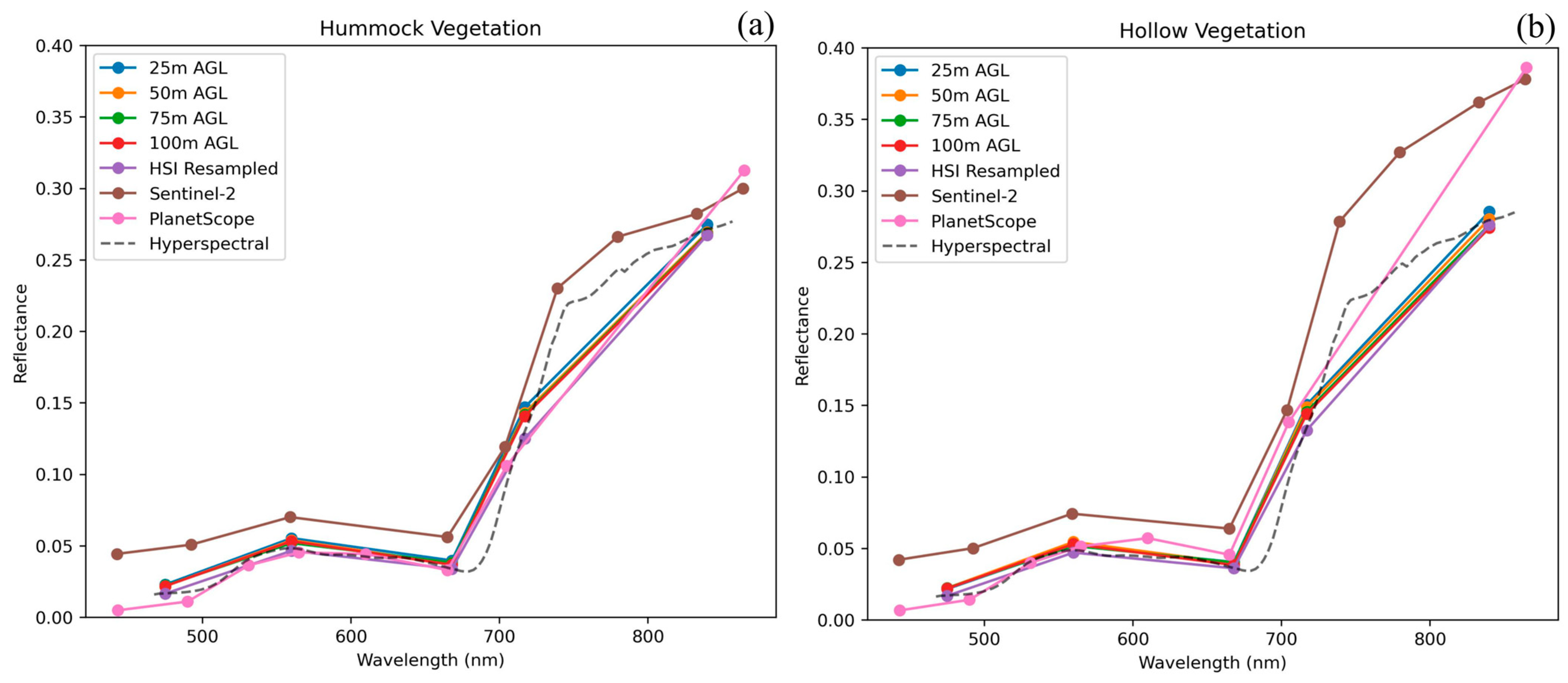
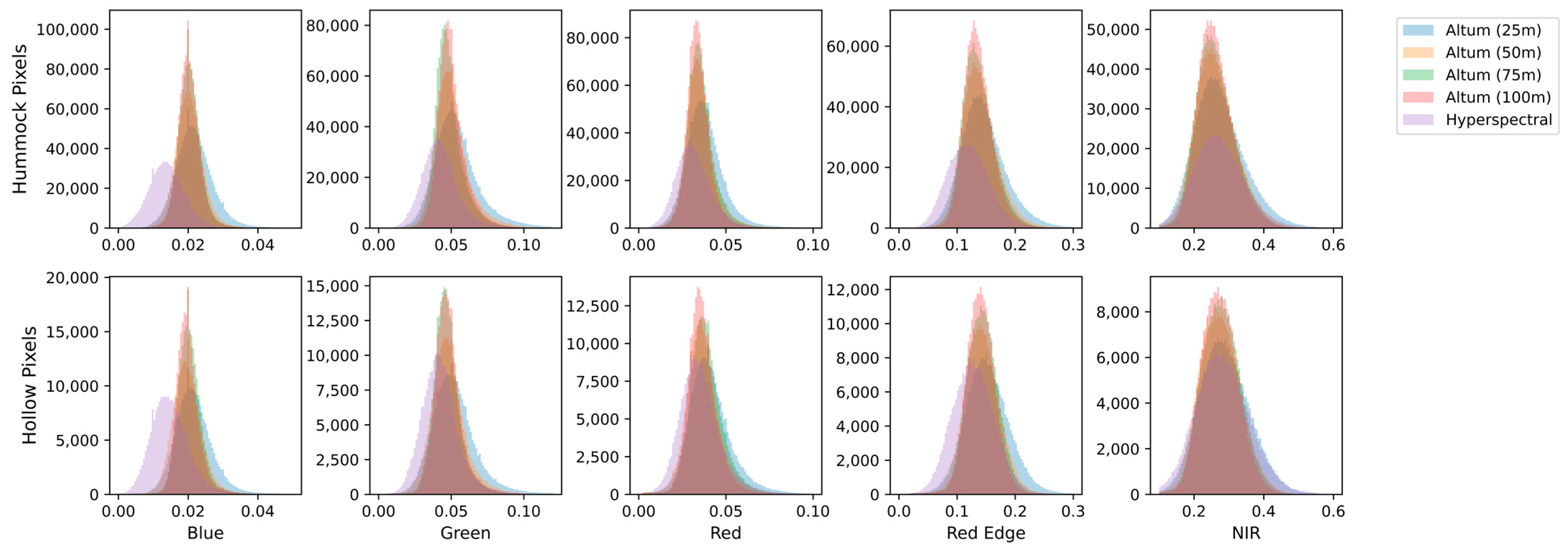
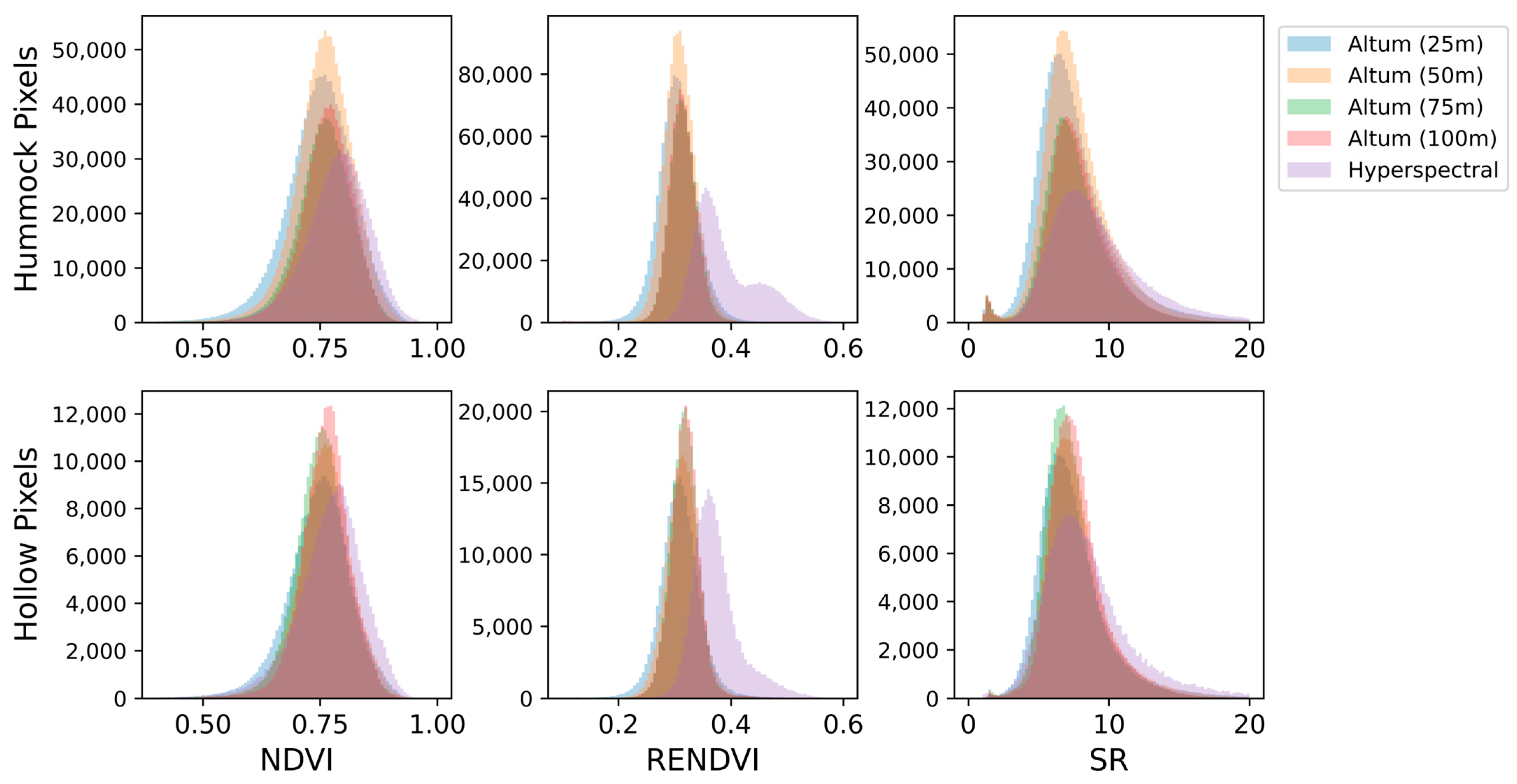
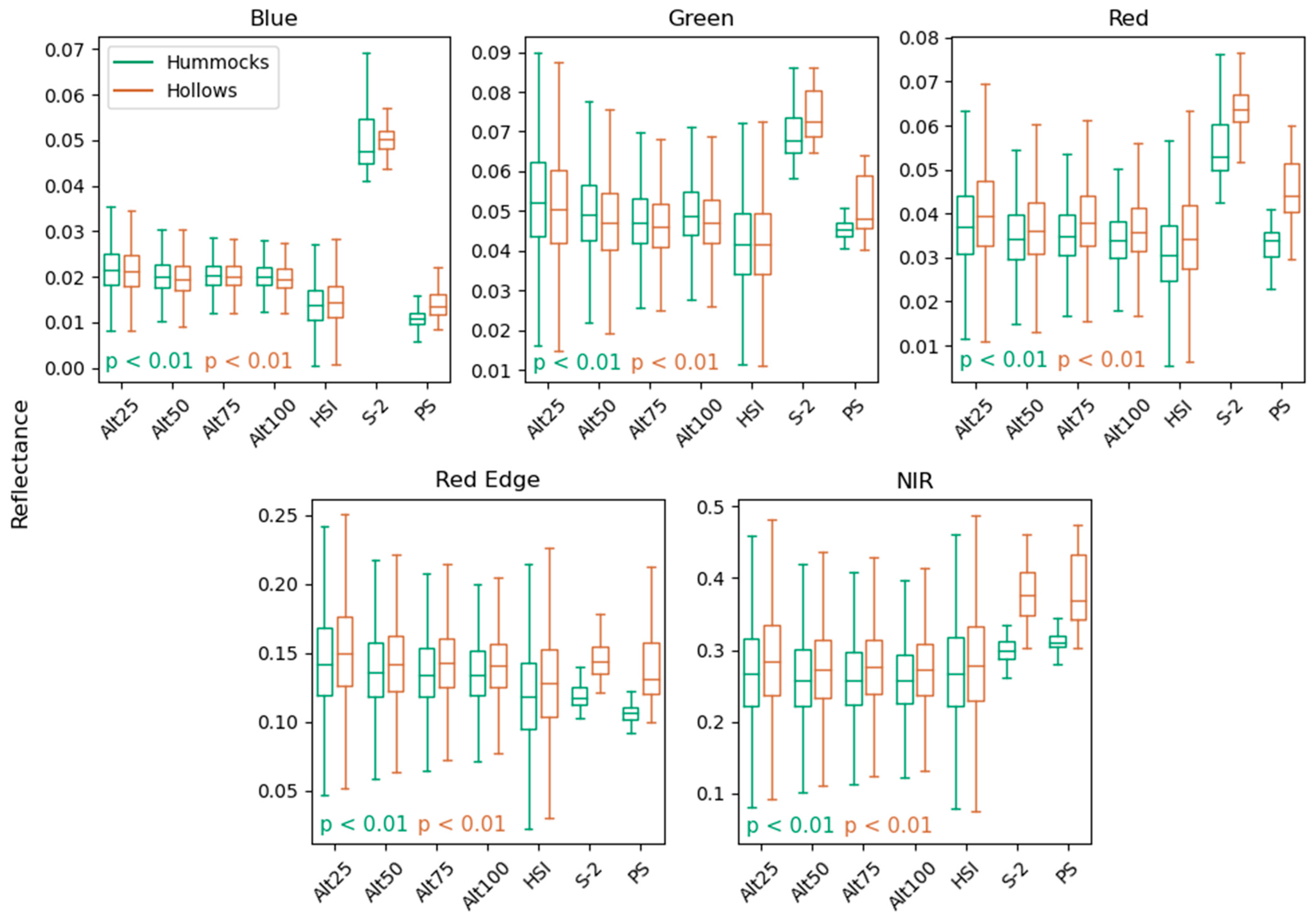
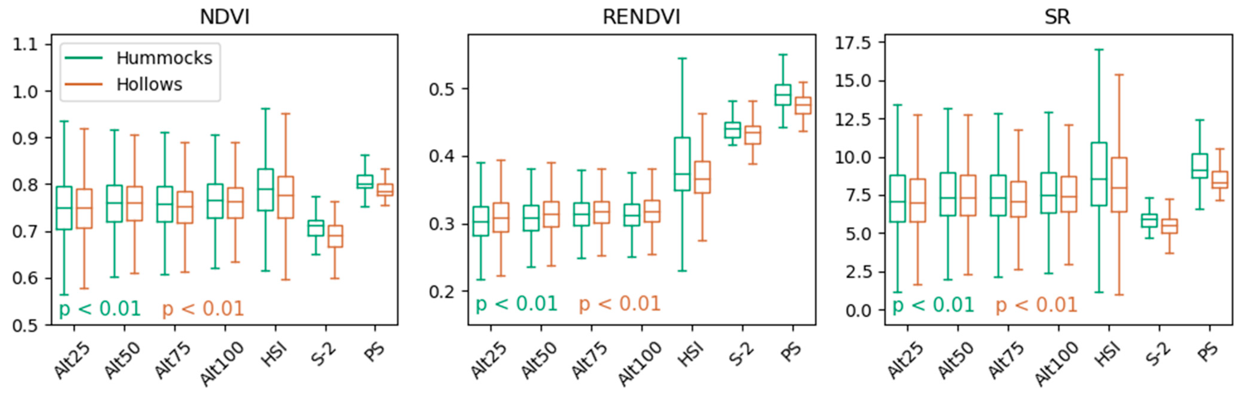
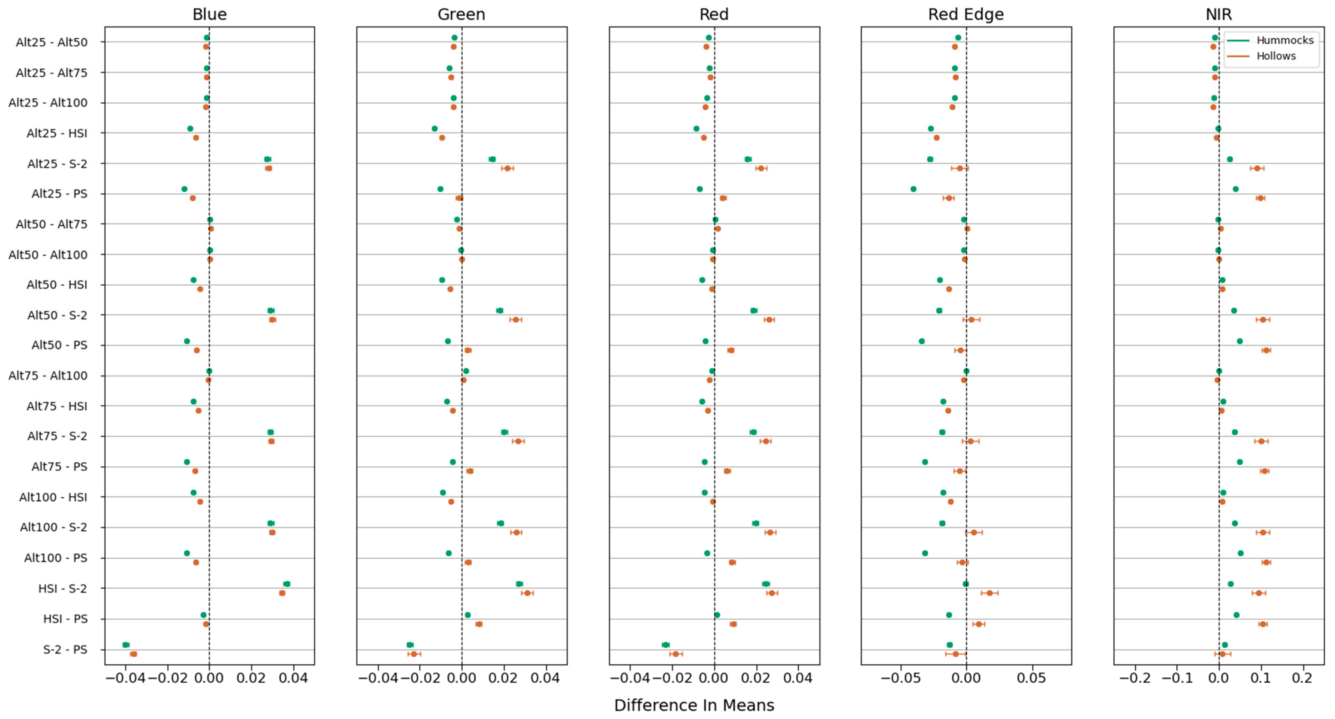
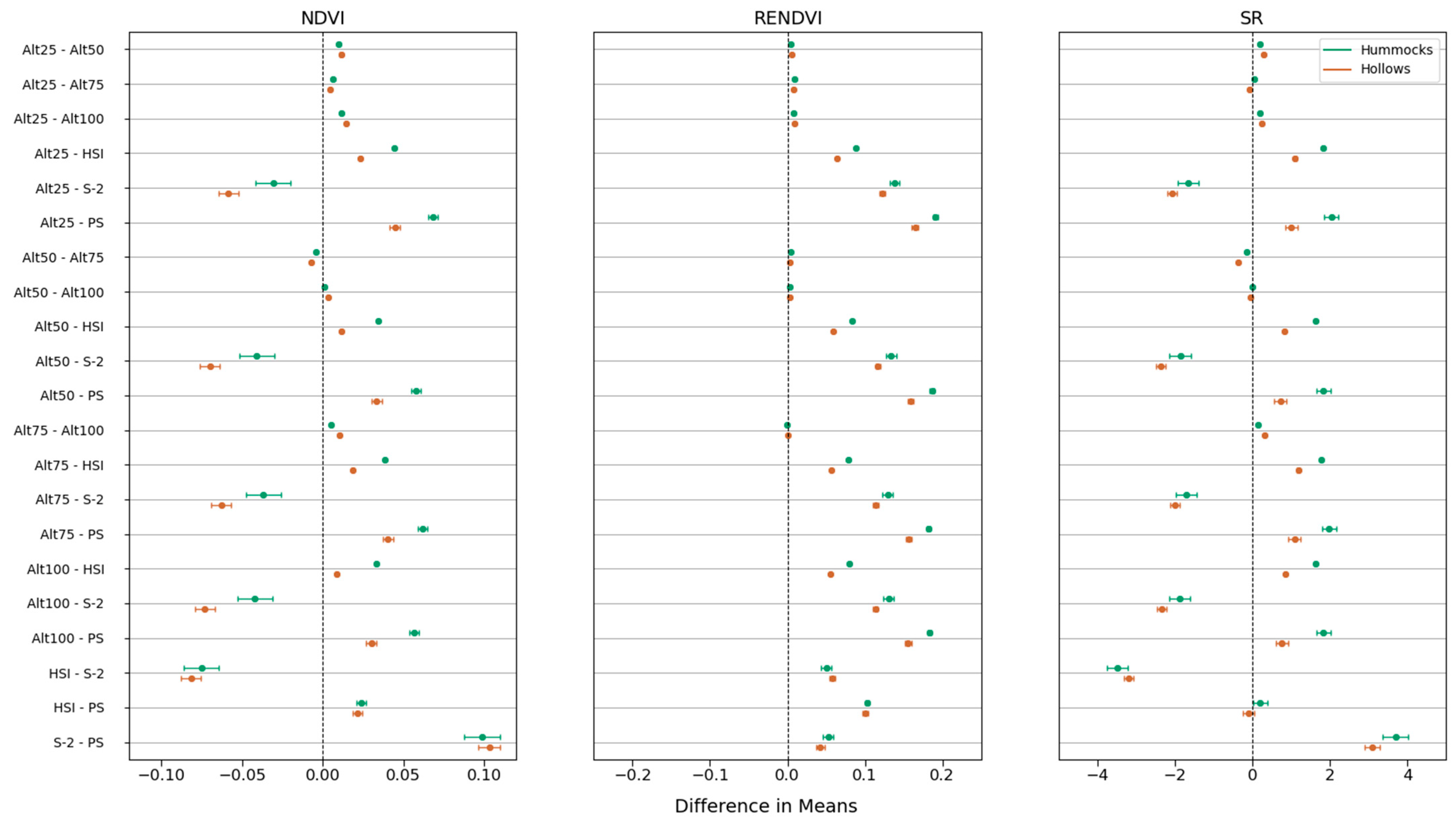
Disclaimer/Publisher’s Note: The statements, opinions and data contained in all publications are solely those of the individual author(s) and contributor(s) and not of MDPI and/or the editor(s). MDPI and/or the editor(s) disclaim responsibility for any injury to people or property resulting from any ideas, methods, instructions or products referred to in the content. |
© 2024 by the authors. Licensee MDPI, Basel, Switzerland. This article is an open access article distributed under the terms and conditions of the Creative Commons Attribution (CC BY) license (https://creativecommons.org/licenses/by/4.0/).