Article

Significant Increase in Global Steric Sea Level Variations over the Past 40 Years

1
State Key Laboratory of Geohazard Prevention and Geoenvironment Protection, Chengdu University of Technology, Chengdu 610059, China
2
College of Earth and Planetary Sciences, Chengdu University of Technology, Chengdu 610059, China
3
School of Geography and Information Engineering, China University of Geosciences (Wuhan), Wuhan 430078, China
4
Shaanxi Key Laboratory of Earth Surface System and Environmental Carrying Capacity, College of Urban and Environmental Sciences, Northwest University, Xi’an 710127, China
*
Author to whom correspondence should be addressed.
Remote Sens. 2024, 16(13), 2466; https://doi.org/10.3390/rs16132466
Submission received: 8 May 2024 / Revised: 19 June 2024 / Accepted: 29 June 2024 / Published: 5 July 2024

Abstract

:
Understanding global sea level variations and exploring their causes hold significant importance for future climate change predictions and the sustainable development of mankind, with the steric sea level (SSL) variations being one of the primary contributors to these changes. Here, we utilize four types of temperature and salinity products (i.e., EN4, IAP, SODA, and GDCSM) to investigate the spatiotemporal characteristics of global SSL changes from 1980 to 2020. We also explore the relationship between SSL changes and the El Niño-Southern Oscillation (ENSO) phenomenon. The findings reveal a rising trend of 0.64–0.97 mm/a in global SSL over the past 40 years, and the annual amplitudes of SSL time series are within the range of 0–50 mm. The SSL trend at a depth of 0–100 m exerts the greatest influence on the overall trend. The ENSO phenomenon has an obvious influence on sea level changes both in the equatorial Pacific region and global scale. The changes in the global sea level (GSL) associated with ENSO are primarily caused by changes in SSL. This study benefits the understanding of SSL changes and their connection to climate change, serves as a reference for comprehensively assessing sea level change mechanisms using diverse datasets and remote sensing technology, and further provides a scientific basis for the sustainable development of mankind in coastal areas.

1. Introduction

The mean rise in global sea level (GSL) resulting from global warming has become an escalating global concern and has drawn more and more attention from scientists and government policymakers. The Sixth Intergovernmental Panel on Climate Change (IPCC) Assessment Report reveals the GSL rose at a rate of 3.7 mm/a from 2006 to 2018 [1,2] and will continue to increase in the future, which is an irrevocable tendency. The GSL changes are primarily induced by variations in seawater volume and mass. Factors like changes in seawater temperature and salinity significantly impact the steric sea level (SSL) variations, while the melting of ice (e.g., land glaciers, Greenland’s ice sheet, and Antarctic ice sheets) due to climate warming is the main driver of global mass sea level (MSL) changes [3]. The rise in seawater temperature stands as a significant contributor to SSL changes, serving as a vital indicator for global climate variations. Studying the SSL changes will help to understand shifts in the global climate system and project future sea level changes, and thus take adaptation strategies.
Advancements in satellite altimetry and gravity satellite technologies have enriched measurements of both GSL and MSL. The ocean temperature and salinity products are the main datasets in the study of SSL changes, which have been widely used in previous studies [4,5]. Yang et al. [6] use multiple sets of satellite altimetry, satellite gravity, and ocean temperature and salinity data to compute the basin-scale sea-level budget from 2005 to 2019 and show that the basin-scale sea level rises significantly at a rate of 1.77–2.39 mm/a, while the steric component explains a ~1 mm/a sea level rise in most ocean basins. Storto et al. [5] involved 20 temperature and salinity products from 1993 to 2010, and illustrated an SSL change trend ranging between 0.1 mm/a and 3.0 mm/a. Zhang et al.’s [7] contrast analyses of two EN4 datasets (i.e., g10, l09) from 1985 to 2005, reveal a heat content discrepancy of about 5 × 10²² J between them, which influences the subsequent computation of SSL changes. Previous studies have predominantly focused on global sea level changes, with limited attention to SSL, particularly in terms of depth. Different temperature and salinity products have different sources and data processing techniques, and thus, result in significant differences when used to derive SSL changes. Additionally, existing research on the mechanisms by which climate change affects sea level change is not sufficiently in-depth.
This study utilizes four mainstream ocean temperature and salinity datasets (i.e., EN4, Gradient-dependent Correlation Scale Method (GDCSM), Simple Ocean Data Assimilation (SODA), Institute of Atmospheric Physics (IAP)) to characterize the spatiotemporal variations of global SSL over the past 40 years (1980 to 2020) and analyzes the relationship between climate change and SSL changes. Specifically, this work aims to: (1) analyze the global SSL from three perspectives—temporal, spatial, and depth—based on different temperature and salinity products; and (2) explore the response of SSL changes to the ENSO phenomenon at various spatial scales. The findings of this study will provide a more complete and comprehensive evaluation of SSL changes and serve as a reference for exploring global sea level changes by combining multi-source data and multi-sensor remote sensing techniques. Furthermore, this study could provide a scientific basis for scientists and policymakers to better develop the coastal areas in the context of global warming.

2. Materials and Methods

2.1. Data

2.1.1. Temperature and Salinity Products

In this study, we employ four temperature and salinity datasets to compute SSL change, including EN4.2.2 (“4.2.2” means the version number, hereinafter referred to as EN4) [8], GDCSM-Argo (a global gridded Argo dataset by using an improved GDCSM, hereinafter referred to as GDCSM) [9], SODA 3.15.2 (“3.15.2” means the version number, hereinafter referred to as SODA) [10], and IAP [11] (Table 1). The EN4 datasets comprise four datasets: c13 [12], c14 [13], g10 [14], and l09 [15] (the first letter like “c” represents the initial of the author’s name and the last two numbers means the year, for example, “13” refers to 2013). These four EN4 datasets differ in applying bias corrections for eXpendable Bathy Thermograph (XBT) and Mechanical Bimetal Thermostat (MBT) [12,13,14,15]. All temperature and salinity datasets have integrated the Argo float dataset with other observational data, except GDCSM data, which is solely based on Argo data, thus resulting in a shorter temporal span (i.e., 2004–2022). Due to the high quality of Argo data between latitudes 60° N and 60°S [16], this oceanic region has been selected as the study area for global sea level research in this work.

2.1.2. Satellite Altimetry Data

The satellite altimetry data, i.e., AVISO, is used to calculate the GSL changes. AVISO integrates measurements from a multitude of altimetry satellites, including Topex/Poseidon, Envisat, ERS-1, ERS-2, Jason-1, Jason-2, Jason-3, Sentinel-3A, Saral, Cryosat-2, GFO, Geosat, and others. Various corrections have been applied to enhance the dataset’s spatial and temporal resolutions compared to individual satellite data, such as ionospheric delay correction, tropospheric wet and dry component correction, solid Earth and ocean tide correction, ocean loading tidal correction, polar tidal correction, electromagnetic bias correction, instrumental correction, inverse barometer correction, and so on [17]. The dataset exhibits a spatial resolution of 0.25° × 0.25°, providing monthly-scale data. AVISO data used in this study is spanning from January 2004 to December 2020.

2.1.3. GRACE-Based Ocean Mass Data

The GRACE and its successor satellite GRACE Follow on (GRACE-FO) were developed by NASA and Deutsches Zentrum fur Luftund Raumfahrt (DLR) for observing changes in the Earth’s gravity field. This study utilized two GRACE/GRACE-FO mass concentration (mascon) blocks data, including Jet Propulsion Laboratory (JPL) mascon (hereafter referred to as JPL_mascon) and the University of Texas Center for Space Research (CSR) mascon (hereafter referred to as CSR_mascon). Mascon products require no post-processing and overcome leakage errors caused by traditional spherical harmonic coefficient filtering, thereby improving estimates of ocean mass changes [18,19]. The JPL_mascon grid data has a spatial resolution of 3° equal area (provided on a 0.5° grid), while the CSR_mascon is 1° equal area (provided on a 0.25° grid). Both data have a temporal resolution of one month. The period used in this study is from January 2004 to December 2020.

2.1.4. ENSO-Associated Indices

ENSO is the collective term for the El Niño phenomenon and the Southern Oscillation, representing changes in seawater temperature and pressure in the equatorial Pacific region. Currently, there is no unified definition or standard for categorizing the occurrences of ENSO cold and warm events in the academic community [20,21,22]. To describe the ENSO phenomenon in this study, the Southern Oscillation Index (SOI), Multivariate ENSO Index (MEI), and the NINO SST Indices, specifically NINO3.4, were utilized. The SOI and MEI are widely used to study factors influencing sea level change [23,24], while the NINO3.4 is the most commonly used for assessing the ENSO phenomenon [25].
The SOI is a time series used to characterize the large-scale sea level pressure (SLP) patterns in the tropical Pacific [26]. The NINO3.4 index is calculated based on sea surface temperature anomalies in the regions spanning latitudes 5°N–5°S and longitudes 170°W−120°W [27]. The MEI is derived from a weighted linear combination of five meteorological variables in the equatorial Pacific Ocean: sea-level pressure, sea surface temperature, zonal and meridional components of the surface wind, sea surface temperature, and outgoing longwave radiation [28].
In this study, El Niño events are designated as any instances where six or more continuous months of NINO3.4 < 0.4, while the opposite is defined as La Niña events, i.e., NINO3.4 > 0.4 for at least six consecutive months. And we use MEI, SOI, and NINO3.4 spanning from January 1980 to December 2020.

2.2. Methods

2.2.1. SSL Calculation

The SSL changes at any arbitrary position in the ocean are obtained by integrating changes in seawater density along the vertical profile [29,30]:
Δ η S S L ( φ , λ ) = 1 ρ 0 h 0 [ ρ ( φ , λ , z , T , S ) ρ ¯ ( φ , λ , z , T ¯ , S ¯ ) ] d z
where φ, λ, and z represent latitude, longitude, and depth, respectively. T   and   S are temperature and salinity, respectively. T ¯   and   S ¯ are their mean values. ρ(φ, λ, z, T, S) mans the density at a specific location of (φ, λ), and the average density is ρ ¯ ( φ , λ , z , T ¯ , S ¯ ) . The constant ρ 0 denotes the average density of seawater, and the value is set to 1028 kg/m3 in this study according to [31]. h is the maximum integration depth, which is set to 1000 m in this study, as variations in temperature and salinity below 1000 m have a negligible impact on SSL [32].
Considering the significant differences in the actual oceanic surface areas at different latitudes, and varying data distributions at different regions, the impact of gridded values across different latitudes to regional averages may not be consistent. Therefore, the regional average values are obtained by weighted averaging for a region, which is expressed as follows:
h ¯ t = λ φ h λ φ t cos ( φ ) λ φ cos ( φ )
where h ¯ t represents the regional average value at time t. λ is longitude. φ is latitude. hλφt denotes the grid cell value located at ( λ , φ ) and at time t. The values calculated at all times will form the time series.

2.2.2. Linear Regression for Time Series

The annual and semi-annual signals from time series data were estimated by linear regression as follows [33]:
Z 0 ( t ) = Z 0 ¯ + a t + C 1 cos 2 π 12 t Φ 1 + C 2 cos 2 π 6 t Φ 2
where Z 0 ( t ) represents the data variation at time t. Z 0 ¯ is the constant term. a is the long-term trend. C 1 and C 2 are the annual and semi-annual amplitude, respectively. Φ 1 and Φ 2 are the annual and semi-annual phases, respectively. The phases are measured in degrees relative to 1 January (0°). The magnitude of the phase reflects the temporal characteristics of sea level variations in a cycle. For example, the later the peak of sea level variations appears, the larger the phase.

2.2.3. Ensemble Empirical Mode Decomposition

Empirical Mode Decomposition (EMD) can decompose non-stationary and non-linear signals into a finite number of Intrinsic Mode Functions (IMFs) and a residual term based on the different amplitude-frequency characteristics, which is widely used to analyze sea level time series [34]. EMD-derived signals exhibit a high signal-to-noise ratio but have a problem of mode mixing, that is, an IMF resulting from EMD decomposition having components of different frequencies. Ensemble Empirical Mode Decomposition (EEMD) is an optimization of the EMD technique [35], which can mitigate the effects of mode mixing by adding noise, enabling the extraction of the different components with different properties more accurately [36]. The EEMD signal decomposition formula is shown as follows:
I ( t ) = m = 1 M   IM F m ( t ) + Res ( t )
where I(t) represents the original input signal. m is the number of IMF, and Res means the residual. The number of IMFs primarily depends on the complexity and variability of the input signals. Specifically, if a signal contains multiple frequency components or significant amplitude variations over time, more IMFs may be obtained during the EEMD process.

2.2.4. Empirical Orthogonal Function

Empirical Orthogonal Function (EOF) is a method for analyzing structural features and extracting principal characteristics in matrix data. EOF partitions the time-varying field into a time-invariant spatial component (i.e., EOFs) and a time-dependent component (i.e., Principal Component (PC)) [37,38,39]:
F m × n = V m × m × P C m × n
where F m × n represents the data that has undergone dimensionality reduction and demeanization. V m × m is the spatial component, while P C m × n corresponds to the temporal component. The m and n represent the dimension of the data. Detailed information about EOF can be seen in Section S3 in Supplementary Material.

3. Results

3.1. SSL Changes Analysis

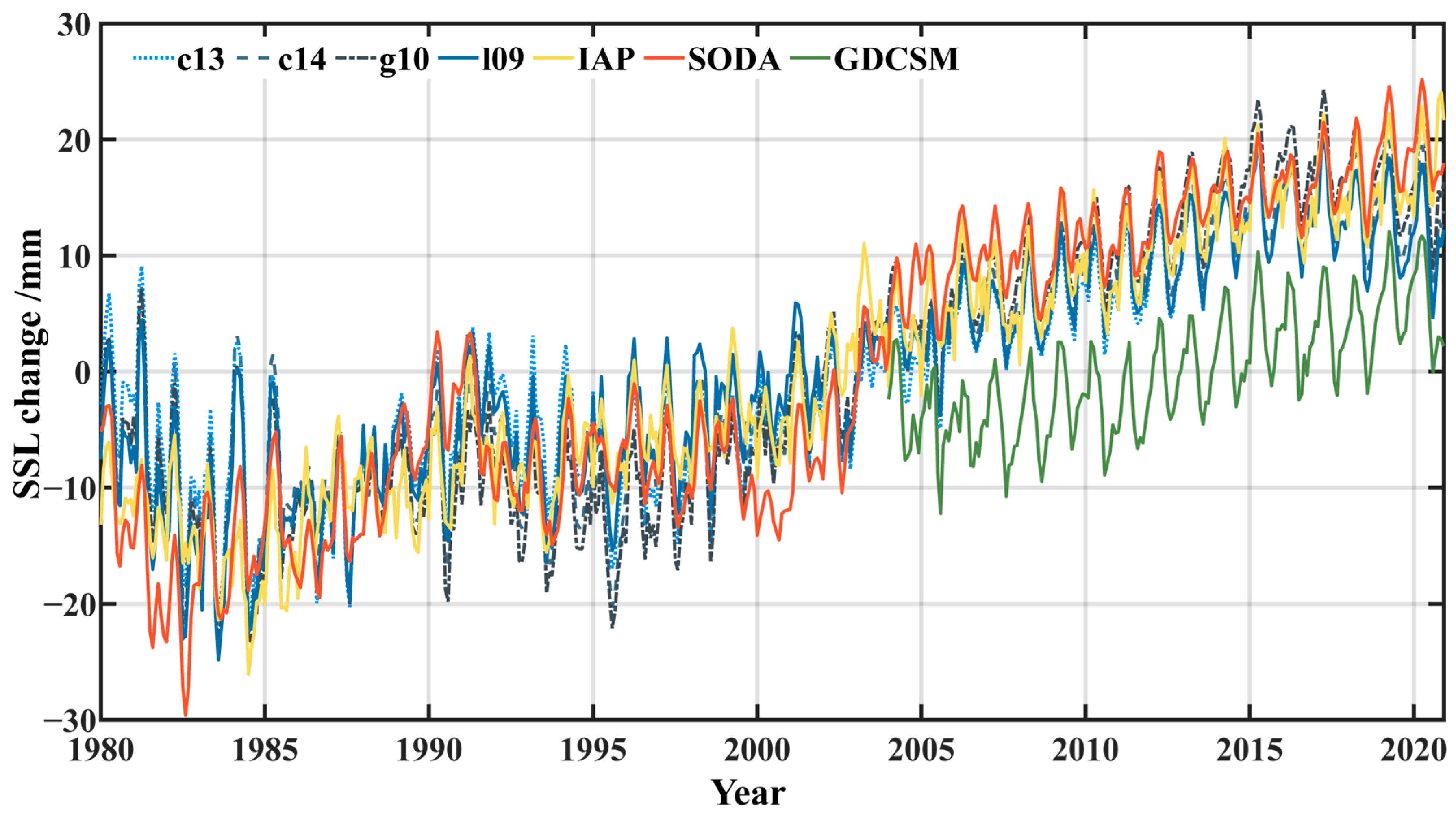
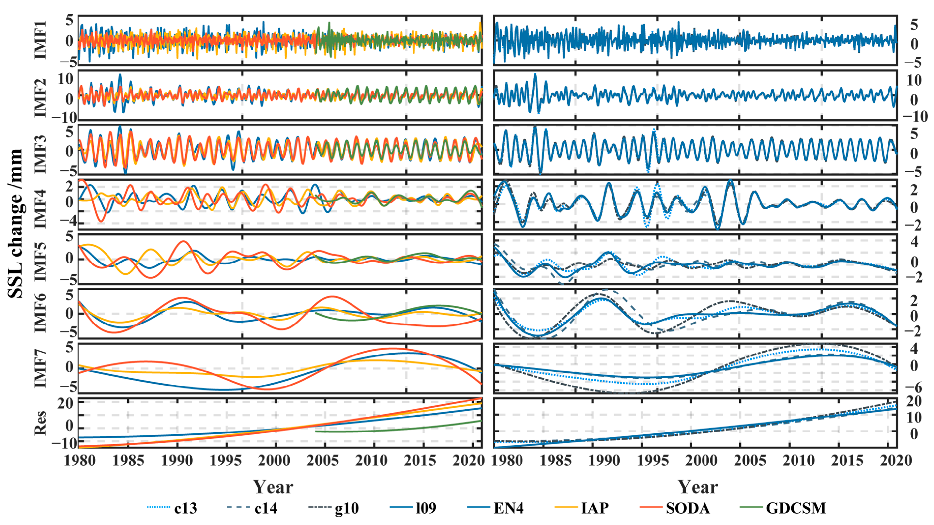
3.1.1. Temporal Characteristics

Figure 1 presents the global mean SSL time series obtained from seven temperature and salinity products (Table 1). They are generally consistent and show a significant upward trend (0.64–0.97 mm/a) (p < 0.01, Table 2). Differences still exist among these time series as they are derived from different products. For example, the degree of uptrends from various products are different. SSL time series based on SODA yield the biggest trend value of 0.97 ± 0.03 mm/a, which is larger by 52% than those using the c13 product (0.64 ± 0.03 mm/a). The annual amplitude differences of SSL derived from different products are in the range of ±1.2 mm, and phase (degrees relative to 1 January (0°), see Section 2.2.2) differences are within ±10°. Compared with the SSL using four products from EN4 (i.e., c13, c14, g10, and l09), those calculated from IAP and SODA products show smaller amplitudes and phases but larger annual trends (Table 2). SSL changes based on the four EN4 products demonstrate generally consistent amplitudes (~4 mm) and phases (~356°) at the annual scale, but exhibit significant differences in annual trends, with the maximum trend value of 0.87 ± 0.04 mm/a (from g10 product) and the minimum of 0.64 ± 0.03 mm/a (from c13 data). SSL derived from GDCSM-Argo shows a remarkable underestimation compared to that using other temperature and salinity products (Figure 1), although its annual trend (0.74 ± 0.05 mm/a) is very close to that from c14 data (0.75 ± 0.03 mm/a).
To gain a detailed understanding of SSL changes across different regions, the global ocean is divided into six zones (Figure 2) [11], including the North Pacific, North Atlantic, Tropical and Subtropical Pacific, Tropical and Subtropical Atlantic, Indian Ocean, and South Ocean. SSLs in all the regions present upward trends (see Table S1 in Supplementary Materials). In high latitudes oceans, including the North Pacific (Figure 2a), North Atlantic (Figure 2b), and South Ocean regions (Figure 2f), SSL exhibits pronounced seasonal variations (see Figure S1 in Supplementary Materials). For the North Pacific (Figure 2a), the SSL time series shows a nearly stable trend from 1980 to 1991, followed by a decreasing trend from 1992 to 2002, and then a rising trend from 2003 to 2020. In the South Ocean region (Figure 2f), SSL experienced a sudden jump in its upward trend around 2004, possibly due to limited Argo measurements before 2004 in this region. While in the equatorial region, like the Tropical and Subtropical Pacific (Figure 2d) and Tropical and Subtropical Atlantic regions (Figure 2e), the SSLs exhibit significant fluctuations in interannual changes but weak seasonal signals (Figure S1 in the Supplementary Materials). In the Indian Ocean region (Figure 2c), SSLs derived from IAP and SODA products show significant differences in the increasing trend, with 1.27 ± 0.08 mm/a for IAP and 0.50 ± 0.07 mm/a for SODA. Also, the four different EN4 products show notable distinct performances in this region (see Table S1 in Supplementary Materials). Overall, SSL calculated from GDCSM consistently underestimates that from other temperature and salinity products in all regions. EN4-derived SSLs perform generally consistently, but the degree of overestimation and underestimation varies among different institutions and different regions.
To conduct a more in-depth analysis of the spatiotemporal features and compare the differences in SSL changes from different temperature and salinity datasets at various time scales, the EEMD is employed to decompose the global SSL change time series (see Figure 1) to obtain the IMFs and residuals (Figure 3). Overall, SSL changes from all products are consistent well in high-frequency signals (i.e., IMF1–IMF3), but different in low-frequency signals (i.e., IMF4–IMF7) in terms of phase and amplitude (Figure 3 (left)). The long-term trend (i.e., the residual component) increased during the study period for SSL based on all products, with trend values ranging from −0.92 mm/a (from SODA) to −0.50 mm/a (from c13). For the SSL changes from four EN4 products (Figure 3 (right)), they are generally consistent in high-frequency signals (i.e., IMF1–IMF4) but exhibit significant differences in decadal annual scale (i.e., IMF5) and lower-frequency variations (i.e., IMF6–IMF7). Regarding the contribution rates of each component to SSL changes (see Table S2 in Supplementary Materials), the long-term trend accounts for ~50% of SSL calculated from most temperature and salinity products. The long-term trend contribution rates are notable differences among different products, with IAP reaching 80% but GDCSM being only ~25%. The secondary contribution rates for SSL changes are the half-year signal (i.e., IMF2) or decadal signal (i.e., IMF7), which shows a lower rate of <10% for the majority of products.

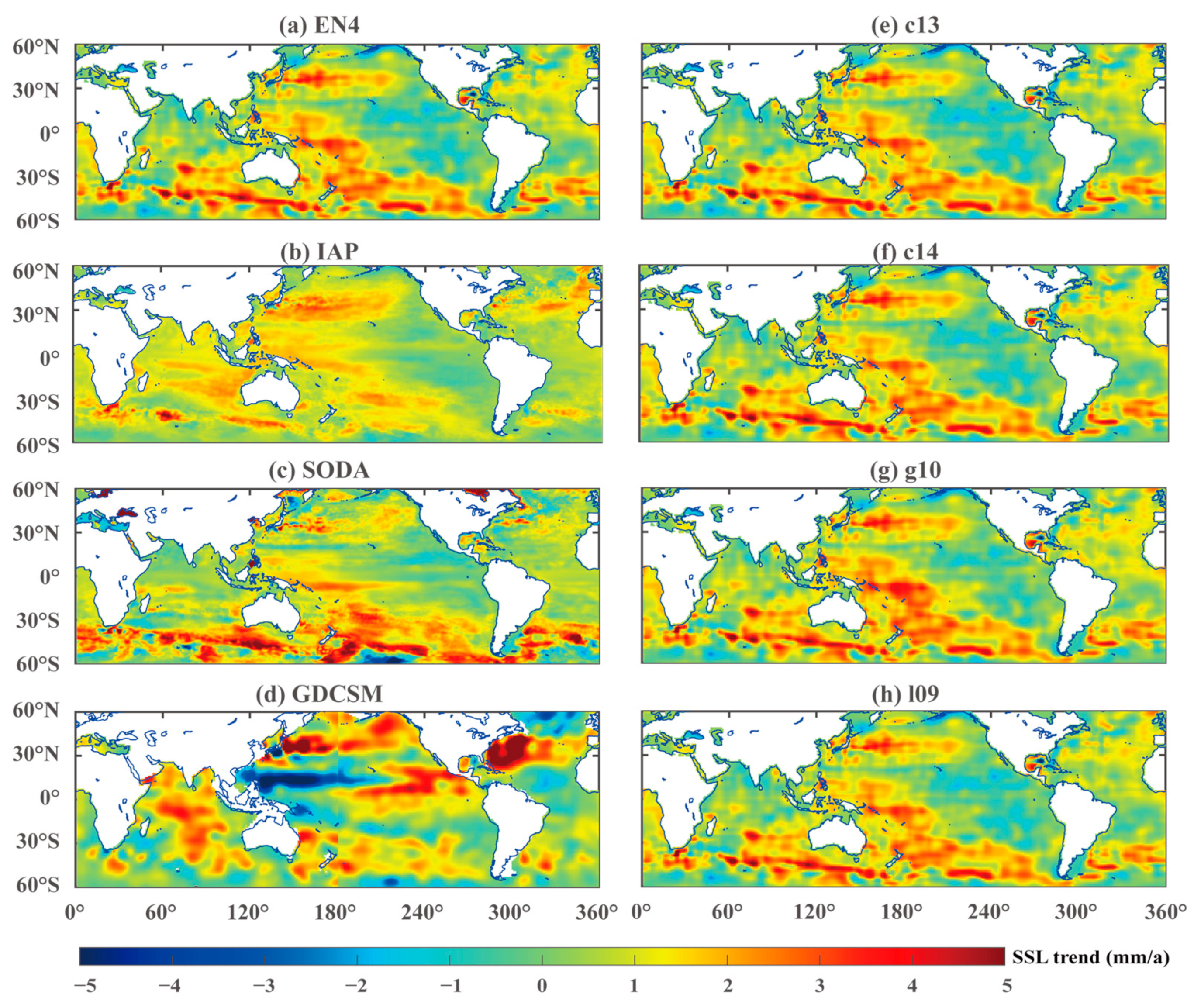
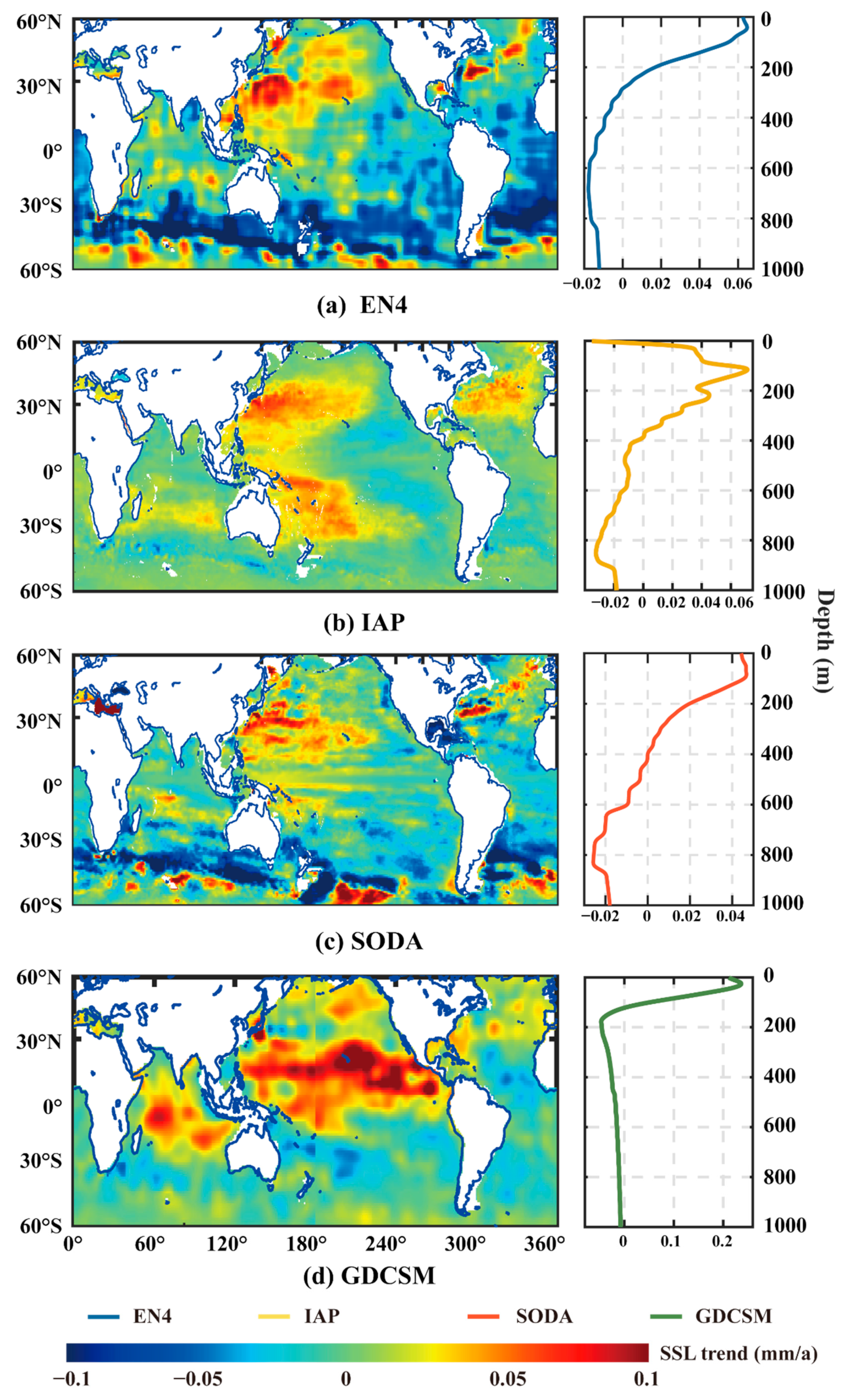
3.1.2. Spatial Distribution

Figure 4 illustrates the spatial distribution of global SSL trends. A rising trend was observed globally in SSL from all the temperature and salinity products, especially in the eastern Indian Ocean, western Pacific, northern South Ocean, and northern Atlantic regions. However, substantial differences exist in SSL trends as they are derived from different products. Comparing the SSL trend using SODA, EN4, and IAP products, the SODA-based SSL trend (Figure 4c) presents the highest value and the IAP-based (Figure 4b) shows the minimum. GDCSM-based SSL trend markedly differs from that derived from other products, revealing a greater rise in global and a distinct descending trend near the equatorial Pacific, contrary to results from other products. SSL trends from EN4’s four datasets exhibit general consistency, lacking obvious spatial disparities (the second column subgraph in Figure 4).
The spatial coverage of different temperature and salinity products varies along coastal and inland seas (Figure 4). EN4 product has the broadest spatial coverage compared to the other three data, encompassing a unique region of the Caspian Sea, which other products lack. However, SODA-based SSL shows an overestimation phenomenon along coastal and inland seas, e.g., the Black Sea, Baltic Sea, China’s Bohai Sea, and Hudson Bay (Figure 4c). GDCSM has the most limited spatial coverage due to its only use of Argo data, resulting in data missing in some areas along coastal and inland seas (Figure 4d). Therefore, it is necessary to consider the spatial coverage of different temperature and salinity products when investigating coastal and inland seas.
The spatial distributions of annual amplitude and phase of SSL changes are detailed in Figures S2 and S3 in Supplementary Materials. The annual amplitude signals of SSL obtained by 7 products (within the range of 0–50 mm) are generally consistent over global seas. Strong annual amplitude signals emerge in some seasonal current regions, like the equatorial warm currents and counter-currents areas in the Pacific North, the Kuroshio region in the northwest Pacific, the Gulf Stream region in the northwest Atlantic, and the south equatorial current and monsoon currents regions in the Indian Ocean, which indicate a substantial correlation between current variations and amplitude magnitude. The annual phases from different products reveal distinct seasonal differences between the northern (neutral phases, equivalent to June–July) and southern hemispheres (high and low phases, equivalent to December–January) (see Figure S2 in Supplementary Materials). Overall, the annual signals of SSL changes from different data sources agree well over global sea areas.

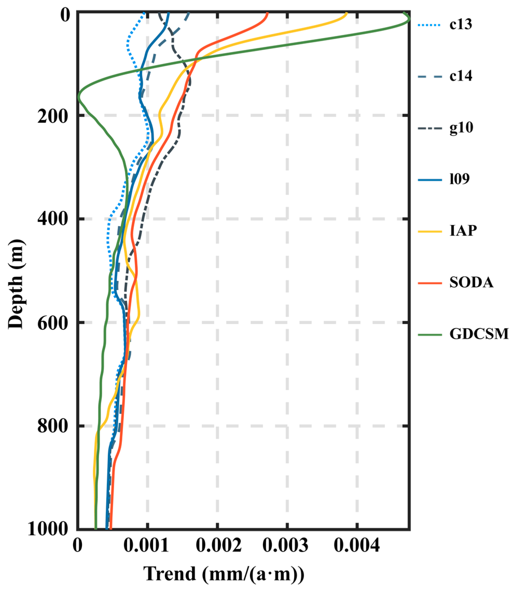
3.1.3. Depth Variations

Figure 5 presents the SSL trend at various depths. The SSL changes for all datasets exhibit positive trends within the depth range of 0–1000 m, indicating that each ocean layer in this range positively contributes to the overall SSL trend. As the depth of the seawater increases, the trend of SSL change gradually decreases. Trends derived from most products peak in the surface layer (0–5 m), except for c13 (peaks in 230–240 m) and g10 (peaks in 130–150 m). The SSL trend derived from GDCSM exhibits significant differences compared to those from other products. It peaks at 0.005 mm/(a·m) and then rapidly declines, approaching nearly 0 mm/(a·m) at a depth of 160 m, rebounding between 160 and 330 m, and then continues to decline slowly. The trends derived from SODA and IAP almost continuously decline slowly after peaking until they stabilize. Compared to other products, the SSL trend of the EN4 product exhibits greater variability. The trends from datasets c13, c14, and l09 each have peaks at depths of 0–5 m, 230–240 m, and 600–650 m, respectively. However, the trends for c14 and l09 peak decrease with increasing depth, while for c13, the trend peaks (0.001 mm/(a·m)) at a depth of 230–240 m. The SSL trend for g10 peaks at around 130 m and then rapidly declines thereafter.
To further investigate the SSL trend variations across different depth layers, we decomposed the SSL trend in-depth sequences (SSL trend at each depth from 0 to 1000 m, with a 1-m interval) using the EOF method. Table 3 shows the first five modes of EOF decomposition results from SSL trend in-depth sequences. The cumulative variance contribution of the first five modes exceeds 90% of SSL trends derived from all four datasets, and the first mode was the primary pattern with a variance contribution ≥ 50%, excepting the SSL trend from the IAP product. Figure 6 shows the first mode of spatial component (i.e., EOF1) and in-depth component (i.e., PC1) from SSL trends derived from the four temperature and salinity products. The first mode of the SSL trends derived from each product mainly occurs within the 0–100 m depth layer. The SSL trends calculated from EN4 and SODA datasets (Figure 6a,c) exhibit a high degree of similarity both in spatial (EOF1) and in-depth (PC1) patterns. A significant downward trend is observed in the northern part of the Southern Ocean. GDCSM-induced SSL trend (Figure 6d) demonstrates that a significant upward trend was observed in the Tropical-subtropical Pacific, the Japan Sea, and the Indian Ocean region. The IAP-derived SSL trend (Figure 6b) presents an inverse trend between the Western Pacific and the Eastern Pacific.

3.2. Relationship between Sea Level Variability and ENSO

3.2.1. Connection between SSL and ENSO in the Equatorial Pacific

Figure 7 shows the global spatial distribution of the correlation coefficient (CC) between SSL changes and MEI, SOI, and NINO3.4 indices. The impact of ENSO on SSL is primarily concentrated in the equatorial Pacific region (i.e., 140°E–80°W and 30°S–30°N, as indicated by the red box in Figure 7). SSL changes exhibit a strong positive correlation with MEI, NINO3.4, and a negative correlation with SOI in the eastern equatorial Pacific, while the opposite phenomenon is observed in the western region. Comparing the SOI, NINO3.4, and MEI indices (Figure 7 and Table S3 in Supplementary Materials), the latter two exhibit a stronger correlation with SSL changes than the former. The primary reason for this phenomenon may be that the SOI is based on SLP data, whereas NINO3.4 and MEI utilize SST data, which has a closer relationship with SSL. A more in-depth investigation is required to understand the detailed reasons behind this correlation, setting the stage for our future research endeavors.
To further explore the relationship between SSL changes and ENSO in the equatorial Pacific, we conduct an EOF analysis on SSL changes derived from different temperature and salinity products (Table 4). The first mode (i.e., PC1) explains over 20% of the variance of all the SSL changes, and the cumulative contribution of the first five modes exceeds 50% of the variance. This reflects that more than half of the spatiotemporal characteristics of SSL changes in the equatorial Pacific region are captured in the first five modes. For the correlation between SSL and ENSO phenomenon, the first mode of SSL changes exhibits a strong correlation with MEI (CC = ~0.8, p < 0.01) according to the temporal and spatial characteristics (Figure S4 in the Supplementary Materials). This demonstrates that the first mode of SSL in the equatorial Pacific is indeed the ENSO mode.

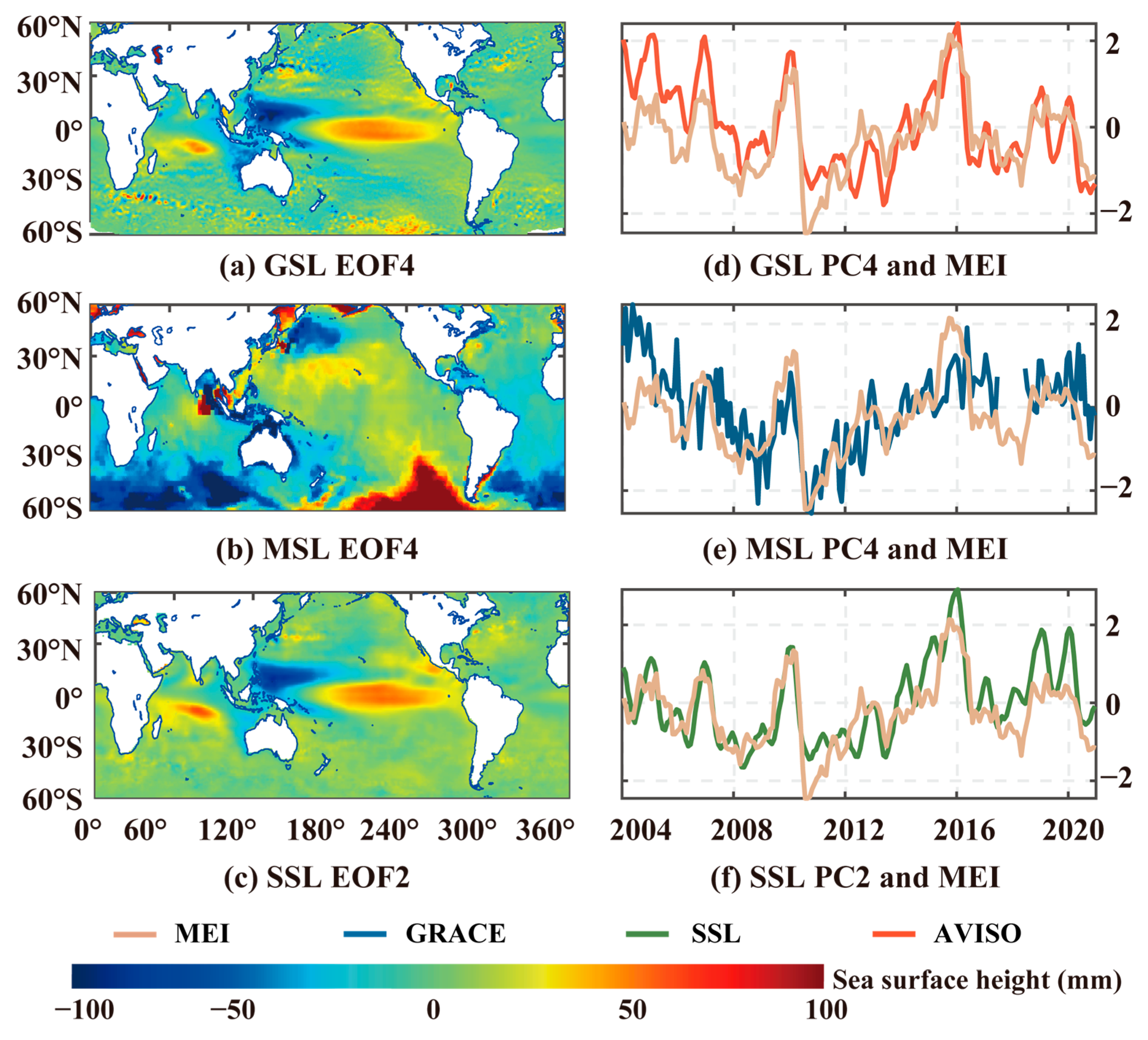
3.2.2. Connection between Sea Level Change and ENSO on a Global Scale

Figure 8 presents the temporal characteristics of the ENSO indices (i.e., NINO3.4 and MEI) and global mean SSL changes. The two opposite phases, El Niño and La Niña, indicate certain changes in both the ocean and the atmosphere. Between 1980 and 2020, ten El Niño events and ten La Niña events were recorded, consistent with the primary ENSO cycle of 2–8 years [40]. Notably, three strong El Niño events occurred in 1982–1983, 1997–1998, and 2015–2016, while the strongest La Niña event during the study period took place in 1999 and persisted for 34 months. On a global scale, the SSL time series does not exhibit an apparent correlation with MEI or SOI indices. But are they completely unrelated on a global scale?
To answer this question, we have investigated the relationships between different components of GSL changes (i.e., steric sea level and mass sea level) and the ENSO-associated index (i.e., MEI). An EOF analysis was conducted on these monthly data sets to obtain the characteristics of different spatial and time-dependent components. From the results in Table 5, it can be observed that PC4 of GSL, PC2 of SSL, and PC4 of MSL are highly correlated with the MEI index, with CC values of 0.70, 0.77, and 0.58, respectively. That is, the second mode of SSL and the fourth mode of GSL and MSL represent the ENSO phenomenon. This suggests the ENSO has an obvious correlation with sea level change on a global scale, not only in the tropical Pacific region. However, the variance contributions are different among these sea level changes. The percentage of variances of PC4 in GSL, PC2 of SSL, and PC4 of MSL are 5.22%, 13.55%, and 3.45%, respectively. This demonstrates that the effect of ENSO on the different components of sea level change is different, and the effect on MSL is the weakest.
Figure 9 depicts spatial and temporal variability of the mode with the strongest correlation with MEI, i.e., EOF4 for GSL, EOF4 for MSL, and EOF2 for SSL. The fourth mode of GSL is primarily driven by the second of SSL. The sea level rises in the equatorial Eastern Pacific and the middle of the Indian Ocean and drops in the equatorial Western Pacific significantly (Figure 9a,c). The occurrence of ENSO leads to significant changes in MSL across the global ocean, not only in the equatorial Pacific. The greatest changes in MSL occur in the Southern Ocean, the Japan Sea, the Southern Bay of Bengal, and Southeast Asian seas. As described in Table 4, the first mode (i.e., PC1) of SSL in the equatorial Pacific is the ENSO mode, and the second model of SSL on a global scale is the ENSO phenomenon (Table 5). This indicates the first PC in the tropical Pacific is the second mode of SSL at a global scale.

4. Discussion

4.1. Comparison of SSL Changes Derived from Different Temperature and Salinity Products

The global SSL changes calculated from 7 temperature and salinity products (i.e., c13, c14, g10, l09, GDCSM, SODA, and IAP) are generally consistent (Figure 1, Figure 2, Figure 3 and Figure 4). Their discrepancies primarily stem from different methods used in handling instrument biases, different construction methods of grid data, various definitions of climatology, and different data sources in data fusing [41,42,43]. EN4 and GDCSM are objective analysis datasets, which are formed from interpolating with climatology and in-situ observations. While IAP and SODA are reanalysis products, which integrate the majority of existing ocean observations (in-situ and remote sensing) with climate models by using data assimilation techniques. The instrument bias correction generally refers to the adjustments of XBT and MBT data. IAP employs the “C14” method to adjust the XBT [13], the same as that used in EN4’s c14 dataset, and uses the IK09 method for MBT correction [44]. While SODA uses the “L09” method to correct the XBT and MBT [15], aligns with that used for EN4’s l09 product.
The discrepancies of SSL time series among various products in different ocean basins (Figure 2) may result from the different quality and quantity of temperature and salinity data. The seasonal characteristics of SSL are obvious in the North Pacific and North Atlantic (Figure S1a,b in Supplementary Materials), and minor differences exist in SSL derived from various products. This is potentially due to the different inherent features of data, e.g., quality and temporal coverage. Moreover, the observational data begins earlier in these two regions (the North Pacific and North Atlantic) (i.e., 1940s) than in other regions, and has broader spatial coverage after 1980 [11,42]. In tropical areas (Figure 2c–e), there are large differences and strong fluctuations in the SSL time series, attributing not only to the difference in data spatial coverage but also to drastic changes in ocean heat content [11]. In the Southern Ocean (Figure 2f), the Argo observation began in 2001, and historical data (before 2001) were supplemented by climatological data, which may lead to the difference compared with other ocean regions.
The SSL derived from 4 EN4 products is generally consistent both in terms of temporal and spatial characteristics (Figure 1 and Figure 2, Table 2). The slight discrepancies among them likely resulted from the “immaturity” of XBT data [15]. That is, the XBT lacks a pressure sensor, and the depth of seawater temperature based on XBT observations relies on a descent speed equation and time of instrument in seawater, which would introduce systematic bias into the XBT data. Moreover, XBT data exhibits constant temperature offsets, and various correction schemes were adopted to address this phenomenon [12,13,14,15]. This is a primary factor contributing to the divergence of SSL calculated by 4 EN4 datasets.
In terms of different ocean depths, notable discrepancies among different products are shown in Figure 5 and Figure 6. The reasons behind the disparities are various. For example, the use of diverse bias correction schemes for the middle depth (i.e., 460–760 m) results from the differences in various EN4 products [42]. Furthermore, different mapping techniques, various merged data sources, and diverse climate models can also lead to discrepancies among different production-induced SSL time series. The high variance contribution rates of the first mode derived from various products (Figure 6 and Table 3) indicate that the spatial distribution characteristics of SSL trends during the 0–100 m depth range are the primary pattern for all depths. However, SSL trends from other depth layers also influence the overall SSL trend. For example, despite its EOF1 variance contribution reaching as high as 89% for SODA, opposite trends are observed in the northern part of the Southern Ocean, indicating that contributions from other depth layers should not be overlooked.

4.2. GSL Variability and Its Response to Climate Change

ENSO is the strongest signal in the interannual variation of the ocean-atmosphere system, whose frequency and intensity are the direct expressions of climate change in the oceans. The occurrence of ENSO signifies anomalies in the wind and precipitation patterns in tropical regions, as well as changes in ocean surface temperature, which are highly relevant to the variations in SSL. Moreover, ENSO can affect global rainfall, leading to water exchange between the continents and the oceans, thereby affecting the changes in MSL. The first mode of SSL in the equatorial Pacific is the ENSO mode (Figure S4), which further highlights the response of SSL to climate variability.
The GSL changes associated with ENSO are primarily caused by changes in SSL (Figure 9 and Table 5). This, to some extent, resolves the issue raised in the previous study [45], in which the authors claimed GSL variations were correlated with ENSO, but the nature of such GSL fluctuations tied to ENSO, whether steric or barystatic, has remained unclear. The fourth mode of MSL shows a high correlation with MEI (CC = 0.58), but the spatial distribution did not present ENSO patterns in the tropical Pacific (Figure 9b). The significant change of MSL in the southern Bay of Bengal (Figure 9b) may be due to uncertainties of GRACE data (e.g., leakage error of land signals). Changes in MSL in other sea areas may be due to the exchange of water between the ocean and land caused by climate changes resulting from the ENSO phenomenon [46]. Detailed mechanism analysis needs further study.
Oceans absorb more than 90% of the excess heat caused by climate change [47]. With global warming intensifying, a range of oceanic crises would occur, such as marine ecosystem disruptions [48], ice caps and ice shelves melting [49], oceanic currents altering [50], and so on. Moreover, climate variations, particularly large-scale climate oscillations, significantly impact GSL annual changes [51] and notably regulate surface mass redistribution [52]. Overall, in the context of climate warming, studying the mechanism of GSL change is particularly important and has become an immense global challenge and endeavor.

4.3. Comparison with Previous Studies

A wealth of findings on sea level variations have been seen in previous research (Table 6). However, most studies have focused on GSL or MSL changes, with fewer investigations centering on SSL variations [4,31,53]. Moreover, existing studies on SSL have primarily relied on Argo-based datasets, which are characterized by lower precision compared to datasets integrating multiple sources [6], and/or short study durations [4,31,52,54]. In this study, we used mainstream types of temperature and salinity products to invert SSL, including a single Argo-based dataset (GDCSM), objective analysis data (EN4), and reanalysis dataset (SODA and IAP). These would yield relatively reliable SSL outcomes. Furthermore, this study covers a broader time span (1980–2020) (Figure 3), allowing us to explore the characteristics of SSL over a long period, such as climatic scales. We also analyze SSL variations at different depths and their contribution to overall SSL, an area rarely investigated in previous studies [55]. Additionally, this study discovered a high correlation between SSL fluctuations and ENSO in the equatorial Pacific region, as well as a correlation between global-scale SSL changes and ENSO. This provides a more comprehensive and in-depth evaluation than previous studies [45].

5. Conclusions

In this study, we examine the global SSL variations from 1980 to 2020 using four types of temperature and salinity products, i.e., EN4, IAP, SODA, and GDCSM and explore the relationship between sea level changes and ENSO phenomenon at various spatiotemporal scales.
The global SSL shows an obvious rising trend at a rate of 0.64–0.97 mm/a from 1980 to 2020. The SSL derived from various temperature and salinity products are generally consistent, especially in high-frequency signals (i.e., IMF1–IMF3). The annual amplitudes of SSL time series are within the range of 0–50 mm, and annual phases reveal distinct seasonal differences between the northern and southern hemispheres. For the depth variations, SSL changes calculated from various datasets exhibit positive trends within the depth range of 0–1000 m, and the SSL trend at the depth of 0–100 m exerts the greatest influence on the overall trend. ENSO phenomenon has an obvious influence on sea level changes both in the equatorial Pacific region and global scale. The changes in the GSL associated with ENSO are primarily caused by changes in SSL.
The limitations of this research are that the ocean depth used (1000 m) is insufficient to capture the full range of SSL variations, and the specific response patterns of SSL to the ENSO phenomenon have not been in-depth analyzed, leaving detailed investigations for future research. Nonetheless, this study provides valuable insights into SSL changes and their response to global warming, thus deepening the understanding of sea level variations. It may also further facilitate the ongoing GSL change mechanism studies using multi-source measurements by improving physical interpretability, with detailed vertical transition mechanism investigations left for future research.

Supplementary Materials

The following supporting information can be downloaded at: https://www.mdpi.com/article/10.3390/rs16132466/s1, Figure S1: Monthly average SSL changes time series estimated by 7 temperature and salinity data in (a) North Pacific, (b) North Atlantic, (c) Indian Ocean, (d) Tropical-subtropical Pacific, (e) Tropical-subtropical Atlantic, and (f) Southern Oceans regions; Figure S2: Annual amplitude of global SSL change; Figure S3: Anniversary phases of global SSL changes. Phases were converted to months according to the formula of “month = phase/30”; Figure S4. The comparison between MEI and EOF1, PC1 of SSL variation derived from the 4 types of temperature and salinity products. EN4 is the average value of its four products including c13, c14, g10, and l09; Table S1: Comparison of the amplitude and phase of the anniversary signals and the trend signals extracted from SSL time series derived from the 7 temperature and salinity products in 6 ocean zones; Table S2: Contribution rates of each component of EEMD decomposition to SSL changes calculated from 7 temperature and salinity products; Table S3: The correlation between MEI, SOI, NINO3.4 and each EOF Mode. EN4 is the average of four datasets, i.e., c13, c14, g10, and l09.

Author Contributions

Conceptualization, Z.S.; Methodology, J.X.; software, J.X.; validation, J.X. and Z.S.; formal analysis, J.X.; investigation, J.X.; resources, Y.Z. and P.S.; data curation, S.Z., Y.X. and L.T.; writing—original draft preparation, J.X.; writing—review and editing, Z.S.; visualization, S.Z.; supervision, Z.S.; project administration, Z.S.; funding acquisition, Z.S. All authors have read and agreed to the published version of the manuscript.

Funding

This research was funded by the National Natural Science Foundation of China (42301049) and the Natural Science Foundation of Sichuan Provincial (2022NSFSC1031, 2024NSFSC0802).

Data Availability Statement

The temperature and salinity data used in this paper can be obtained based on Section 2.1.1. The GRACE JPL_mascon and CSR_mascon data used in this study are available at https://podaac.jpl.nasa.gov/dataset/TELLUS_GRAC-GRFO_MASCON_CRI_GRID_RL06.1_V3 (accessed on 7 June 2023) and https://www2.csr.utexas.edu/grace/RL06_mascons.html (accessed on 27 June 2023), respectively; Satellite altimetry data is obtained from the websites of https://www.aviso.altimetry.fr/en/data.html (accessed on 3 April 2023). The NINO3.4,MEI and SOI data used in this study are available at https://psl.noaa.gov/gcos_wgsp/Timeseries/Nino34/ (accessed on 5 June 2024), https://crudata.uea.ac.uk/cru/data/soi/ (accessed on 25 August 2023) and https://psl.noaa.gov/enso/mei/ (accessed on 25 August 2023), respectively.

Acknowledgments

Thanks to the constructive comments given by three anonymous reviewers, which are very helpful for the improvement of the manuscript. Thanks to the open availability of observational datasets.

Conflicts of Interest

The author declares no conflicts of interest.

References

  1. Hua, L.; Xiao, C.; Yan, Z.; Yu, Y.; Zhang, T. Interpretation of IPCC AR6 report: Monitoring and Projections of Global and Regional Sea Level Change. Adv. Clim. Chang. Res. 2022, 18, 12–18. [Google Scholar] [CrossRef]
  2. IPCC. Climate Change 2021: The Physical Science Basis; Masson-Delmotte, V., Zhai, P., Pirani, A., Connors, S.L., Péan, C., Berger, S., Caud, N., Chen, Y., Goldfarb, L., Gomis, M.I., et al., Eds.; Cambridge University Press: Cambridge, UK, 2021. [Google Scholar] [CrossRef]
  3. Chen, M.; Chang, M.; Zhang, W.; Jia, Y.; Zuo, C. Characteristics of Low-frequency Variation of Global Steric Sea Level. Adv. Mar. Sci. 2016, 34, 162–174. [Google Scholar] [CrossRef]
  4. Royston, S.; Vishwakarma, B.D.; Westaway, R.; Rougier, J.; Sha, Z.; Bamber, J. Can We Resolve the Basin-Scale Sea Level Trend Budget From GRACE Ocean Mass? J. Geophys. Res.-Ocean. 2020, 125, 16. [Google Scholar] [CrossRef]
  5. Storto, A.; Masina, S.; Balmaseda, M.; Guinehut, S.; Xue, Y.; Szekely, T.; Fukumori, I.; Forget, G.; Chang, Y.S.; Good, S.A.; et al. Steric sea level variability (1993–2010) in an ensemble of ocean reanalyses and objective analyses. Clim. Dyn. 2017, 49, 709–729. [Google Scholar] [CrossRef]
  6. Yang, Y.Y.; Feng, W.; Zhong, M.; Mu, D.P.; Yao, Y.L. Basin-Scale Sea Level Budget from Satellite Altimetry, Satellite Gravimetry, and Argo Data over 2005 to 2019. Remote Sens. 2022, 14, 4637. [Google Scholar] [CrossRef]
  7. Zhang, M.; Zhao, C.; Zhang, Y.; Jiang, W.; Wang, G. Discrepancies in the Ocean Heat Content of Two EN4 Products. Adv. Mar. Sci. 2020, 38, 390–399. [Google Scholar]
  8. Good, S.A.; Martin, M.J.; Rayner, N.A. EN4: Quality controlled ocean temperature and salinity profiles and monthly objective analyses with uncertainty estimates. J. Geophys. Res. Ocean. 2013, 118, 6704–6716. [Google Scholar] [CrossRef]
  9. Zhang, C.L.; Wang, D.Y.; Liu, Z.H.; Lu, S.L.; Sun, C.H.; Wei, Y.L.; Zhang, M.X. Global Gridded Argo Dataset Based on Gradient-Dependent Optimal Interpolation. J. Mar. Sci. Eng. 2022, 10, 650. [Google Scholar] [CrossRef]
  10. Carton, J.A.; Chepurin, G.A.; Chen, L.G. SODA3: A New Ocean Climate Reanalysis. J. Clim. 2018, 31, 6967–6983. [Google Scholar] [CrossRef]
  11. Cheng, L.J.; Trenberth, K.E.; Fasullo, J.; Boyer, T.; Abraham, J.; Zhu, J. Improved estimates of ocean heat content from 1960 to 2015. Sci. Adv. 2017, 3, e1601545. [Google Scholar] [CrossRef]
  12. Cowley, R.; Wijffels, S.; Cheng, L.; Boyer, T.; Kizu, S. Biases in Expendable Bathythermograph Data: A New View Based on Historical Side-by-Side Comparisons. J. Atmos. Ocean. Technol. 2013, 30, 1195–1225. [Google Scholar] [CrossRef]
  13. Cheng, L.; Zhu, J.; Cowley, R.; Boyer, T.; Wijffels, S. Time, Probe Type, and Temperature Variable Bias Corrections to Historical Expendable Bathythermograph Observations. J. Atmos. Ocean. Technol. 2014, 31, 1793–1825. [Google Scholar] [CrossRef]
  14. Gouretski, V.; Reseghetti, F. On depth and temperature biases in bathythermograph data: Development of a new correction scheme based on analysis of a global ocean database. Deep Sea Res. Part I Oceanogr. Res. Pap. 2010, 57, 812–833. [Google Scholar] [CrossRef]
  15. Levitus, S.; Antonov, J.I.; Boyer, T.P.; Locarnini, R.A.; Garcia, H.E.; Mishonov, A.V. Global ocean heat content 1955-2008 in light of recently revealed instrumentation problems. Geophys. Res. Lett. 2009, 36, 5. [Google Scholar] [CrossRef]
  16. Wei, F.; Min, Z. Global sea level variations from altimetry, GRACE and Argo data over 2005–2014. Geod. Geodyn. 2015, 6, 274–279. [Google Scholar]
  17. Minster, J.; Cazenave, A.; Serafini, Y.; Mercier, F.; Gennero, M.; Rogel, P. Annual cycle in mean sea level from Topex–Poseidon and ERS-1: Inference on the global hydrological cycle. Glob. Planet Chang. 1999, 20, 57–66. [Google Scholar] [CrossRef]
  18. Save, H.; Bettadpur, S.; Tapley, B.D. High-resolution CSR GRACE RL05 mascons. J. Geophys. Res.-Solid Earth 2016, 121, 7547–7569. [Google Scholar] [CrossRef]
  19. Watkins, M.M.; Wiese, D.N.; Yuan, D.N.; Boening, C.; Landerer, F.W. Improved methods for observing Earth’s time variable mass distribution with GRACE using spherical cap mascons. J. Geophys. Res. Solid Earth 2015, 120, 2648–2671. [Google Scholar] [CrossRef]
  20. Chen, H.; Xu, F.; Li, X.; Xia, T.; Zhang, Y. Intensities and time-frequency variability of enso in the last 65 years. J. Trop. Meteorol. 2017, 33, 683–694. [Google Scholar] [CrossRef]
  21. Li, X.; Zhai, P. On indices and indicators of ENSO episodes. Acta Meteorol. Sin. 2000, 58, 102–109. [Google Scholar] [CrossRef]
  22. Zhao, Y.; Chen, Y. Classification and Cycles of ENSO Events Over the Past Century. Trans. Oceanol. Limnol. 1998, 12, 7–13. [Google Scholar]
  23. Xi, H.; Zhang, Z.Z.; Lu, Y.; Li, Y. Long-Term and Interannual Variation of the Steric Sea Level in the South China Sea and the Connection with ENSO. J. Coast. Res. 2019, 35, 489–498. [Google Scholar] [CrossRef]
  24. Zhong, Y.; Zhong, M.; Feng, W. Monitoring the cause of global mean sea level with satellite gravity and analyzing the correlation with ENSO in recent decade. Prog. Geophys. 2016, 31, 643–648. [Google Scholar]
  25. GB/T 33666-2017; El Niño/La Niña Event Identification Methods. Standardization Administration of the People’s Republic of China: Beijing, China, 2017; p. 2.
  26. Ropelewski, C.F.; Jones, P.D. An extension of the Tahiti-Darwin Southern Oscillation Index. Mon. Weather Rev. 1987, 115, 2161–2165. [Google Scholar] [CrossRef]
  27. Trenberth, K.E.; Stepaniak, D.P. Indices of El Nino evolution. J. Clim. 2001, 14, 1697–1701. [Google Scholar] [CrossRef]
  28. Zhang, T.; Hoell, A.; Perlwitz, J.; Eischeid, J.; Murray, D.; Hoerling, M.; Hamill, T.M. Towards Probabilistic Multivariate ENSO Monitoring. Geophys. Res. Lett. 2019, 46, 10532–10540. [Google Scholar] [CrossRef]
  29. Chen, J.L.; Wilson, C.R.; Tapley, B.D.; Famiglietti, J.S.; Rodell, M. Seasonal global mean sea level change from satellite altimeter, GRACE, and geophysical models. J. Geod. 2005, 79, 532–539. [Google Scholar] [CrossRef]
  30. Fofonoff, N.P.; Millard, R.C. Algorithms for Computation of Fundamental Properties of Seawater; UNESCO Technical Papers in Marine Sciences; UNESCO: Paris, France, 1983; 53p. [Google Scholar] [CrossRef]
  31. Wang, F.W.; Shen, Y.Z.; Chen, Q.J.; Sun, Y. Reduced misclosure of global sea-level budget with updated Tongji-Grace2018 solution. Sci. Rep. 2021, 11, 17667. [Google Scholar] [CrossRef]
  32. Dhomps, A.L.; Guinehut, S.; Le Traon, P.Y.; Larnicol, G. A global comparison of Argo and satellite altimetry observations. Ocean Sci. 2011, 7, 175–183. [Google Scholar] [CrossRef]
  33. Torres, R.R.; Tsimplis, M.N. Seasonal sea level cycle in the Caribbean Sea. J. Geophys. Res.-Ocean. 2012, 117, 18. [Google Scholar] [CrossRef]
  34. Ezer, T.; Corlett, W.B. Analysis of relative sea level variations and trends in the Chesapeake Bay: Is there evidence for acceleration in sea level rise? In Proceedings of the 2012 Oceans, Hampton Roads, VA, USA, 14–19 October 2012; pp. 1–5. [Google Scholar] [CrossRef]
  35. Wu, Z.; Huang, N.E. Ensemble empirical mode decomposition: A noise-assisted data analysis method. Adv. Adapt Data Anal. 2011, 1, 1–41. [Google Scholar] [CrossRef]
  36. Wu, S.; Liu, Z.Y.; Zhang, R.; Delworth, T.L. On the observed relationship between the Pacific Decadal Oscillation and the Atlantic Multi-decadal Oscillation. J. Oceanogr. 2011, 67, 27–35. [Google Scholar] [CrossRef]
  37. Preisendorfer, R.W. Principal Component Analysis in Meteorology and Oceanography; Elsevier: Amsterdam, The Netherlands, 1988; pp. 212–214. [Google Scholar]
  38. North, G.R.; Bell, T.L.; Cahalan, R.F.; Moeng, F.J. Sampling errors in the estimation of empirical orthogonal functions. Mon. Weather Rev. 1982, 110, 699–706. [Google Scholar] [CrossRef]
  39. Nerem, R.S.; Rachlin, K.E.; Beckley, B.D. Characterization of global mean sea level variations observed by TOPEX/POSEIDON using empirical orthogonal functions. Surv. Geophys. 1997, 18, 293–302. [Google Scholar] [CrossRef]
  40. Torrence, C.; Webster, P.J. Interdecadal changes in the ENSO-monsoon system. J. Clim. 1999, 12, 2679–2690. [Google Scholar] [CrossRef]
  41. Boyer, T.; Domingues, C.M.; Good, S.A.; Johnson, G.C.; Lyman, J.M.; Ishii, M.; Gouretski, V.; Antonov, J.; Wijffels, S.; Church, J.A.; et al. Sensitivity of Global Upper-Ocean Heat Content Estimates to Mapping Methods, XBT Bias Corrections, and Baseline Climatologies. J. Clim. 2016, 29, 4817–4842. [Google Scholar] [CrossRef]
  42. Abraham, J.P.; Baringer, M.; Bindoff, N.L.; Boyer, T.; Cheng, L.; Church, J.A.; Conroy, J.L.; Domingues, C.M.; Fasullo, J.T.; Gilson, J. A review of global ocean temperature observations: Implications for ocean heat content estimates and climate change. Rev. Geophys. 2013, 51, 450–483. [Google Scholar] [CrossRef]
  43. Cheng, L.; Zhu, J.; Abraham, J. Global Upper Ocean Heat Content Estimation: Recent Progress and the Remaining Challenges. Atmos. Ocean. Sci. Lett. 2015, 8, 333–338. [Google Scholar] [CrossRef]
  44. Ishii, M.; Kimoto, M. Reevaluation of historical ocean heat content variations with time-varying XBT and MBT depth bias corrections. J. Oceanogr. 2009, 65, 287–299. [Google Scholar] [CrossRef]
  45. Piecuch, C.G.; Quinn, K.J. El Nino, La Nina, and the global sea level budget. Ocean Sci. 2016, 12, 1165–1177. [Google Scholar] [CrossRef]
  46. Boening, C.; Willis, J.K.; Landerer, F.W.; Nerem, R.S.; Fasullo, J. The 2011 La Nina: So strong, the oceans fell. Geophys. Res. Lett. 2012, 39, 5. [Google Scholar] [CrossRef]
  47. von Schuckmann, K.; Palmer, M.D.; Trenberth, K.E.; Cazenave, A.; Chambers, D.; Champollion, N.; Hansen, J.; Josey, S.A.; Loeb, N.; Mathieu, P.P.; et al. An imperative to monitor Earth’s energy imbalance. Nat. Clim. Chang. 2016, 6, 138–144. [Google Scholar] [CrossRef]
  48. Hawkings, J.R.; Wadham, J.L.; Tranter, M.; Lawson, E.; Sole, A.; Cowton, T.; Tedstone, A.J.; Bartholomew, I.; Nienow, P.; Chandler, D.; et al. The effect of warming climate on nutrient and solute export from the Greenland Ice Sheet. Geochem. Perspect. Lett. 2015, 1, 94–104. [Google Scholar] [CrossRef]
  49. Etourneau, J.; Sgubin, G.; Crosta, X.; Swingedouw, D.; Willmott, V.; Barbara, L.; Houssais, M.N.; Schouten, S.; Damsté, J.S.S.; Goosse, H. Ocean temperature impact on ice shelf extent in the eastern Antarctic Peninsula. Nat. Commun. 2019, 10, 304. [Google Scholar] [CrossRef]
  50. McManus, J.F.; Francois, R.; Gherardi, J.M.; Keigwin, L.D.; Brown-Leger, S. Collapse and rapid resumption of Atlantic meridional circulation linked to deglacial climate changes. Nature 2004, 428, 834–837. [Google Scholar] [CrossRef] [PubMed]
  51. Cazenave, A.; Dieng, H.B.; Meyssignac, B.; von Schuckmann, K.; Decharme, B.; Berthier, E. The rate of sea-level rise. Nat. Clim. Chang. 2014, 4, 358–361. [Google Scholar] [CrossRef]
  52. Mu, D.P.; Xu, T.H.; Guan, M.Q. Sea level instantaneous budget for 2003–2015. Geophys. J. Int. 2022, 229, 828–837. [Google Scholar] [CrossRef]
  53. Chen, J.L.; Tapley, B.; Wilson, C.; Cazenave, A.; Seo, K.W.; Kim, J.S. Global Ocean Mass Change From GRACE and GRACE Follow-On and Altimeter and Argo Measurements. Geophys. Res. Lett. 2020, 47, e2020GL090656. [Google Scholar] [CrossRef]
  54. Amin, H.; Bagherbandi, M.; Sjöberg, L.E. Quantifying barystatic sea-level change from satellite altimetry, GRACE and Argo observations over 2005–2016. Adv. Space Res. 2020, 65, 1922–1940. [Google Scholar] [CrossRef]
  55. Li, Z.A.; Chen, J.; Li, J.; Hu, X. Temporal and Spatial Variations of Global Steric Sea Level Change from Argo Observations, 2005–2015. J. Geod. Geodyn. 2018, 38, 923–929. [Google Scholar] [CrossRef]
  56. Barnoud, A.; Pfeffer, J.; Guérou, A.; Frery, M.L.; Siméon, M.; Cazenave, A.; Chen, J.; Llovel, W.; Thierry, V.; Legeais, J.F. Contributions of Altimetry and Argo to Non-Closure of the Global Mean Sea Level Budget Since 2016. Geophys. Res. Lett. 2021, 48, e2021GL092824. [Google Scholar] [CrossRef]
Figure 1. Global monthly mean SSL changes time series derived from 7 temperature and salinity products from 1980 to 2020.
Remotesensing 16 02466 g001
Figure 2. Monthly average SSL changes time series estimated by 7 temperature and salinity Data in (a) North Pacific, (b) North Atlantic, (c) Indian Ocean, (d) Tropical-subtropical Pacific, (e) Tropical-subtropical Atlantic, and (f) Southern Oceans regions. All time series have been smoothed to eliminate seasonal variations.
Remotesensing 16 02466 g002
Figure 3. IMFs from SSL decomposed by EEMD. (Left): SSL changes from 4 temperature and salinity data including GDCSM, SODA, IAP, and EN4, where EN4 is the average of 4 datasets (i.e., c13, c14, g10, l09); (Right): EN4’s 4 datasets. EN4, IAP, and SODA are decomposed into 7 IMFs and a residual term, while GDCSM-Argo is decomposed into 6 IMFs and a residual term. IMF1−IMF3 represent characteristics at 4 months (seasonal scale), 7 months (semi-annual scale), and 12 months (annual scale), respectively. Residual (Res) represents a long-term trend.
Remotesensing 16 02466 g003
Figure 4. Global SSL Trends derived from different temperature and salinity products, including (a) EN4, (b) IAP, (c) SODA, (d) GDCSM, (e) c13, (f) c14, (g) g10, and (h) l09. The first column presents results from four types of products, with EN4 representing the average of its four datasets. The second column displays the SSL trend computed from EN4’s four products.
Remotesensing 16 02466 g004
Figure 5. Global mean SSL annual trends derived from different temperature and salinity products at the depth range of 0–1000 m. The ocean depth is stratified by 1-m intervals. Latitude-weighted averaging (see Formula (2)) is used to calculate the regional average value in each ocean layer, depicting the average seawater volumetric changes at various depths. Formula (3) is employed to extract the trend signals for each SSL time series.
Remotesensing 16 02466 g005
Figure 6. The EOF1 and PC1 of SSL trend derived from the 4 types of temperature and salinity products, including (a) EN4, (b) IAP, (c) SODA, and (d) GDCSM. EN4 is the average value of its four products including c13, c14, g10, and l09. The left column of the horizontal axis represents the depth of seawater from 0 to 1000 m. EN4, IAP, and SODA calculate SSL trends from 1980 to 2020, and GDCSM calculates SSL trends from 2004 to 2020.
Remotesensing 16 02466 g006
Figure 7. Global spatial distribution of correlation coefficients between global SSL changes and ENSO indices, including SOI (A), NINO 3.4 (B), and MEI (C).
Remotesensing 16 02466 g007
Figure 8. Temporal characteristics of ENSO indices (i.e., SOI and MEI) and the global SSL changes, alongside the El Niño and La Niña events depicted in red and blue, respectively.
Remotesensing 16 02466 g008
Figure 9. The spatial and temporal variability of the strongest correlation modes with MEI, including spatial characteristics of (a) GSL EOF4, (b) MSL EOF4, and (c) SSL EOF2, and temporal variability of (d) GSL PC4 and MEI, (e) MSL PC4 and MEI, and (f) SSL PC2 and MEI.
Remotesensing 16 02466 g009
Table 1. Temperature and salinity products used in this work.
DatasetsPeriodSpatial Coverage Horizontal
Resolution
Vertical
Resolution
Raw DataBackground FieldAssimilation Method
EN41900−Present180°W–180°E, 83°S–89°N1° × 1°42 Layers from 5 to 5350 mWOD18, Argo,
GTSPP, ASBO
WOA98Optimal interpolation
GDCSM2004–2022179.5°W–179.5°E, 89.5°S–89.5°N1° × 1°58 Layers from 0 to 2000 mArgoMulti-year monthly mean analysis fieldGradient-dependent correlation scale method
SODA1980–2020180°W–180°E, 75°S–90°N0.5° × 0.5°50 Layers from 0 to 5500 mWOD13,
SST
CM2.5 coupled modelComputationally efficient optimal interpolation
IAP1960–Present180°W–180°E, 90°S–90°N1° × 1°24 Layers from 0 to 2000 mWOD18Climate model ensemble mean fieldEnsemble optimal interpolation
Note: WOD18 is World Ocean Database in 2018 and WOD13 means World Ocean Database in 2013. GTSPP is the Global Temperature and Salinity Profile Program. ASBO is Arctic Synoptic Basin Wide Oceanography. WOA98 means World Ocean Atlas in 1998.
Table 2. Comparison of annual amplitude, phase, and trend of SSL changes calculated from 7 salinity-temperature data. The magnitude reflects the temporal characteristics of sea level variations in a cycle, and the phase is measured in degrees relative to 1 January (0°).
DatasetAnnualLinear
Trend (mm/a)
Amplitude (mm)Phase (deg)
EN4c134.06 ± 0.56356.08 ± 7.850.64 ± 0.03
c143.98 ± 0.56356.17 ± 8.080.75 ± 0.03
g104.09 ± 0.65356.90 ± 9.160.87 ± 0.04
l094.01 ± 0.45354.94 ± 6.430.71 ± 0.03
IAP2.99 ± 0.38342.71 ± 7.280.89 ± 0.02
SODA3.24 ± 0.58345.92 ± 10.180.97 ± 0.03
GDCSM4.11 ± 0.35347.15 ± 4.850.74 ± 0.05
Table 3. Percentage of variance explained by the EOF modes (PC1–PC5) from SSL trend in-depth sequences derived from different products. EN4 is the average of four datasets, i.e., c13, c14, g10, and l09.
EOF ModesEN4-Derived SSL TrendIAP-Derived SSL TrendSODA-Derived SSL TrendGDCSM-Derived SSL Trend
Percentage of Variance (%)Percentage of Variance (%)Percentage of Variance (%)Percentage of Variance (%)
PC162.137.889.049.8
PC215.330.15.330.4
PC38.08.82.87.0
PC45.47.21.54.9
PC52.56.20.93.6
Table 4. Percentage of variance explained by the EOF modes (PC1–PC5) from SSL changes derived from different monthly means products and the CC between MEI and each EOF Mode. EN4 is the average of four datasets, i.e., c13, c14, g10, and l09.
EOF ModesEN4-Derived SSLIAP-Derived SSLSODA-Derived SSLGDCSM-Derived SSL
Percentage of
Variance (%)
CCPercentage of
Variance (%)
CCPercentage of
Variance (%)
CCPercentage of
Variance (%)
CC
PC124.50.8624.00.7821.40.8527.10.80
PC213.2−0.1216.60.4011.60.0715.80.32
PC310.80.2014.20.0611.10.2812.2−0.11
PC45.10.066.5−0.154.80.075.8−0.04
PC54.8−0.104.3−0.054.2−0.023.60.05
Table 5. Percentage of variance explained by the EOF modes (PC1–PC5) from monthly means sea level changes (including GSL, SSL, and MSL) and the CC between MEI and each EOF Mode. SSL is the average of four datasets, i.e., EN4, SODA, IAP, and GDCSM. MSL is the average of JPL_mascon and CSR_mascon. The period is from January 2004 to December 2020.
EOF ModesGSLSSLMSL
Percentage of Variance (%)CCPercentage of Variance (%)CCPercentage of Variance (%)CC
PC112.9−0.3029.30.0746.10.17
PC29.30.1913.60.7716.5−0.02
PC35.50.368.20.316.50.03
PC45.20.705.7−0.223.50.58
PC52.40.193.80.202.20.30
Table 6. Comparison with previous studies.
SourceTime SpanData SourcesSSL Trend (mm/a)
This study2003–2020EN4 (c13, c14, g10, l09), IAP, SODA, GDCSM0.90 ± 0.06
Mu et al. [52]2003–2015JAMSTEC, EN4, BOA-Argo1.13 ± 0.12
Amin et al. [54]2005–2016IPRC, JAMSTEC, SIO, EN4, CSIO1.20 ± 0.07
Wang et al. [31]2005–2016IPRC, SIO1.16 ± 0.08
Chen et al. [53]2005–2020SIO, IPRC, JAMSTEC1.00 ± 0.22
Yang et al. [6]2005–2019BOA-Argo, CORA, IAP, IPRC, JAMSTEC, NCEI, SIO, EN4 (g10, l09)1.05 ± 0.14
Royston et al. [4]2005–2015SIO, EN4(g14), ISAS15, JAMSTEC0.96 ± 0.08
Barnoud et al. [56]2005–2019NOAA, EN4, SCRIPPS, JAMSTEC1.07 ± 0.08
Note: JAMSTEC is the Japan Agency for Marine-Earth Science and Technology. BOA-Argo represents the Global Ocean Argo gridded data set. IPRC is the International Pacific Research Center. SIO means Scripps Institution of Oceanography. CSIO is the Chinese Second Institute of Oceanography. CORA represents the Coriolis Ocean Dataset for Reanalysis. NCEI means National Centers for Environmental Information. ISAS15 refers to the In Situ Analysis System version 15. NOAA is the National Oceanic and Atmospheric Administration. SCRIPPS means Scripps Institution of Oceanography.
Disclaimer/Publisher’s Note: The statements, opinions and data contained in all publications are solely those of the individual author(s) and contributor(s) and not of MDPI and/or the editor(s). MDPI and/or the editor(s) disclaim responsibility for any injury to people or property resulting from any ideas, methods, instructions or products referred to in the content.

