Abstract
Ice, Cloud, and Land Elevation Satellite-2 (ICESat-2) has excellent potential for obtaining water depth information around islands and reefs. Combining the density-based spatial clustering of applications with noise algorithm (DBSCAN) and multiscale quadtree analysis, we propose a new photon-counting lidar denoising method to discard the large amount of noise in ICESat-2 data. First, the kernel density estimation (KDE) is used to preprocess the point cloud data, and a threshold is set to remove the noise photons on the sea surface. Next, the DBSCAN algorithm is used to preliminarily remove underwater noise photons. Then, the quadtree segmentation and Otsu algorithm are used for fine denoising to extract accurate bottom signal photons. Based on ICESat-2 pho-ton-counting data from six typical islands and reefs worldwide, the proposed method outperforms other algorithms in terms of denoising effect. Compared to in situ data, the determination coefficient (R2) reaches 94.59%, and the root mean square error (RMSE) is 1.01 m. The proposed method can extract accurate underwater terrain information, laying a foundation for offshore bathymetry.
1. Introduction
Bathymetric topography is fundamental to understanding the ocean. Obtaining bathymetric information in shallow water is highly important for shipping safety and marine engineering [1,2]. Satellite-derived bathymetry (SDB) provides high temporal and spatial resolution [3] and is an effective means of obtaining shallow water depth information [4,5,6]. However, high-precision in situ water depth control points are necessary for SDB. Currently, methods to obtain in situ water depth control points include shipborne multibeam echo-sounder systems (MBES), shipborne single-beam echo-sounder systems (SBES), and airborne LiDAR bathymetric systems (ALB). However, due to water depth limitations, the measurement efficiency of shipborne acoustic measurement systems is significantly reduced, while ALBs are expensive and only suitable for small-scale measurements. Fortunately, spaceborne LiDAR offers a new way to obtain in situ water depth control points. In September 2018, the Ice, Cloud, and Land Elevation Satellite-2 (ICESat-2), which was launched by the National Aeronautics and Space Administration (NASA) of the United States, began obtaining in situ water depth control points. Studies show that satellites can retrieve a maximum water depth of 38 m [7].
ICESat-2 is equipped with the Advanced Topographical Laser Altimeter System (ATLAS), employing micropulse multibeam photon-counting LiDAR technology with a higher pulse repetition rate, more accurate precision, and a smaller laser irradiation range [8,9]. ICESat-2 orbits height of approximately 500 km, an observation coverage of 88°S~88°N, a repetition period of 91 days, and 1387 orbits in each cycle. The ATLAS system emits six single-pulse laser beams (532 nm) at a repetition rate of 10 kHz, arranged in parallel in three groups along the orbit. The ratio of strong to weak pulse energy stands at 4:1. Although ICESat-2 performs well in many areas, a large amount of noise exists in the collected data [10]. Therefore, studying the problem of ICESat-2 data denoising is highly important for subsequent related research.
Many scholars have studied photon point cloud denoising. The denoising algorithm based on grid image processing converts the photon point cloud into a two-dimensional image. Image processing technology eliminates the noise points in photon data. The standard algorithm for this purpose is the Canny algorithm [11]. For example, Chen et al. [12] extracted signal photons based on Gaussian filtering and gradient descent algorithms to identify features in raster data products. Magruder et al. [13] enhanced upon the traditional Canny edge detection algorithm and obtained ideal denoising results. However, the raster image processing algorithm may lead to accuracy loss in the conversion process, which affects the denoising effect. The denoising algorithm based on local statistical parameters removes noise by calculating the threshold of the local statistical parameters of the photons. Herzfeld et al. [14] proposed a denoising algorithm based on spatial statistical parameters that separates signal points from noise points by setting parameter thresholds. Gwenzi et al. [15] proposed a density-cutting method based on point cloud elevation statistics and verified it with Mabel data and simulation data. However, parameter threshold selection restricts the denoising effect of local statistical parameter algorithms.
Currently, the photon denoising algorithm mainly depends on density clustering analysis. Signal photons can be distinguished from noise photons by setting an appropriate search radius and neighborhood points [16,17]. The central density clustering algorithms comprise density-based spatial clustering of applications with noise (DBSCAN) [18] and ordering points to identify the clustering structure (OPTICS) [19]. Zhang et al. [20] improved the DBSCAN clustering algorithm and employed horizontal ellipses to cluster signal photons. However, this method requires excessively high input parameters and performs poorly in mountainous areas. Xie et al. [21] proposed an ellipse search method and adaptive direction method that exhibits high terrain adaptability. Chen et al. [22] proposed a photon point cloud denoising algorithm based on an elliptic local outlier factor and showed that the shape of the search area significantly impacts the denoising results. Ma et al. [23] proposed a formula for calculating minimum point (MinPts) parameters based on the DBSCAN algorithm but did not describe the calculation method for epsilon (EPS) parameters. Zhu et al. [24] proposed the ellipse search options algorithm that distinguishes signal photons and noise by the maximum interclass variance, but the ellipse search radius still requires manual input. Zhang et al. [25] proposed a quadtree nonparametric input denoising method that uses quadtrees to separate photons and employs the photon layer value to characterize the photon density. However, this method performed well only in the simulation data denoising experiment. Huang et al. [26] proposed a fusion denoising method based on the local outlier factor and inverse distance metric, which can effectively extract sparse signal photons from ICESat-2 data. However, the signal extraction performance is suboptimal in deep water regions. Song et al. [27] proposed an adaptive signal photon extraction and classification algorithm that effectively processes ICESat-2 data in mixed regions of complex terrain and water without requiring auxiliary data. Xie et al. [28] proposed a water depth-adaptive submarine photon extraction method using the KNN distance ratio. However, in high-noise environments, this method is limited. Limited research exists on the denoising of shallow water area data collected by ICESat-2 [29], and it is essential to explore an efficient and reasonable shallow water area denoising algorithm.
In summary, the existing ICESat-2 denoising algorithm has limitations and requires further study and improvement due to its universality, simplicity, and stability. Therefore, this paper proposes a quadtree denoising algorithm based on multiscale analysis. The innovations presented in this paper are as follows:
- KDE separates sea surface photons to mitigate the poor denoising effect and low efficiency caused by the uneven density of sea surface photons and seafloor photons;
- A method to divide the window of seafloor photons according to density is proposed, and data denoising is conducted from the perspective of multiscale analysis to eliminate the influence of different water depths and terrains on the denoising performance;
- The pre-judged strategy is added to the quadtree segmentation algorithm, and prejudgments are performed before segmentation to eliminate the problem of misjudging high-value noise points as signal points.
The remainder of this article is structured as follows. First, the experimental data and validation data are detailed. Then, the feasibility of the denoising algorithm is proven by experiments, and the superiority of the proposed method is illustrated from the perspective of photon density and terrain characteristics. Finally, the performances of different denoising algorithms are assessed for different water depths, and corresponding conclusions are presented.
2. Materials and Methods
2.1. Study Area
This study uses signal extraction and noise processing for shallow water areas around islands and reefs. The selected research areas include Oahu Island in the Hawaiian Islands, Dongdao Island and Huaguang Reef in the South China Sea, and Ailinginae Atoll in the Marshall Islands. Due to their unique geographical characteristics and environmental conditions, these areas are significant for studying sea level change, marine dynamics, and ecosystems.
- Oahu Island, one of the main islands in the Hawaiian Islands, covers an area of 1574 km2. Honolulu, the State’s capital, and Pearl Harbor and Waikiki beaches are located on the island. Oahu is famous for its spectacular coastline and changeable submarine topography;
- Dongdao Island is located in the Dongdao Island atoll east of the Xuande Islands. The island has a long strip shape, with a length of approximately 2400 m, a width of approximately 1000 m, and a land area of approximately 1.7 km2;
- Huaguang Reef is in the Yongle Archipelago, Xisha Islands, China. It is 31 km long from east to west and 12 km wide from south to north. It is a hidden reef in the water. At low tide, the atoll can be exposed above the sea;
- Ailinginae Atoll is a coral atoll in the Republic of the Marshall Islands. It is located north of the Ralik chain islands. It has a typical annular coral reef structure with an area of approximately 2.8 km2. Atolls provide a unique perspective for studying sea level change and its impact on coral reef ecosystems.
The above experimental areas were selected based on their geographical characteristics, climatic environment, and other factors and have a certain universality. This study explores more advanced denoising algorithms to improve the application accuracy and efficiency of ICESat-2 satellite data in water depth inversion.
2.2. Data
2.2.1. ICESat-2 ATL03 Dataset
The primary data source used in this paper is NASA’s ATL03 V006 data product. ATL03 is a level-2 data product containing each received photon’s precise latitude, longitude, and elevation information. This paper selects six study areas, and the details are shown in Table 1.

Table 1.
Experimental area.
The location information of the study area is shown in Figure 1. The six selected study areas have good water quality, and the laser has good water permeability. The study areas are far from each other to avoid the influence of geological correlation, and the seafloor topography changes significantly, including that of laser beams from different periods with different strengths. The selection of research data is diverse, which can verify the effectiveness of the method in this paper from multiple angles and intuitively verify the universality of the denoising algorithm utilized in this paper.
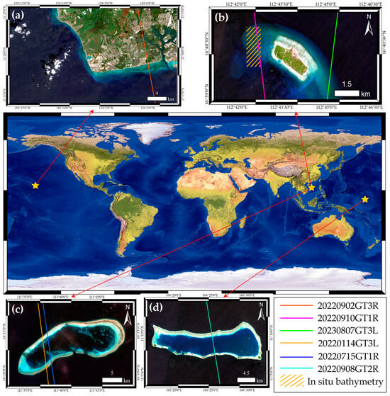
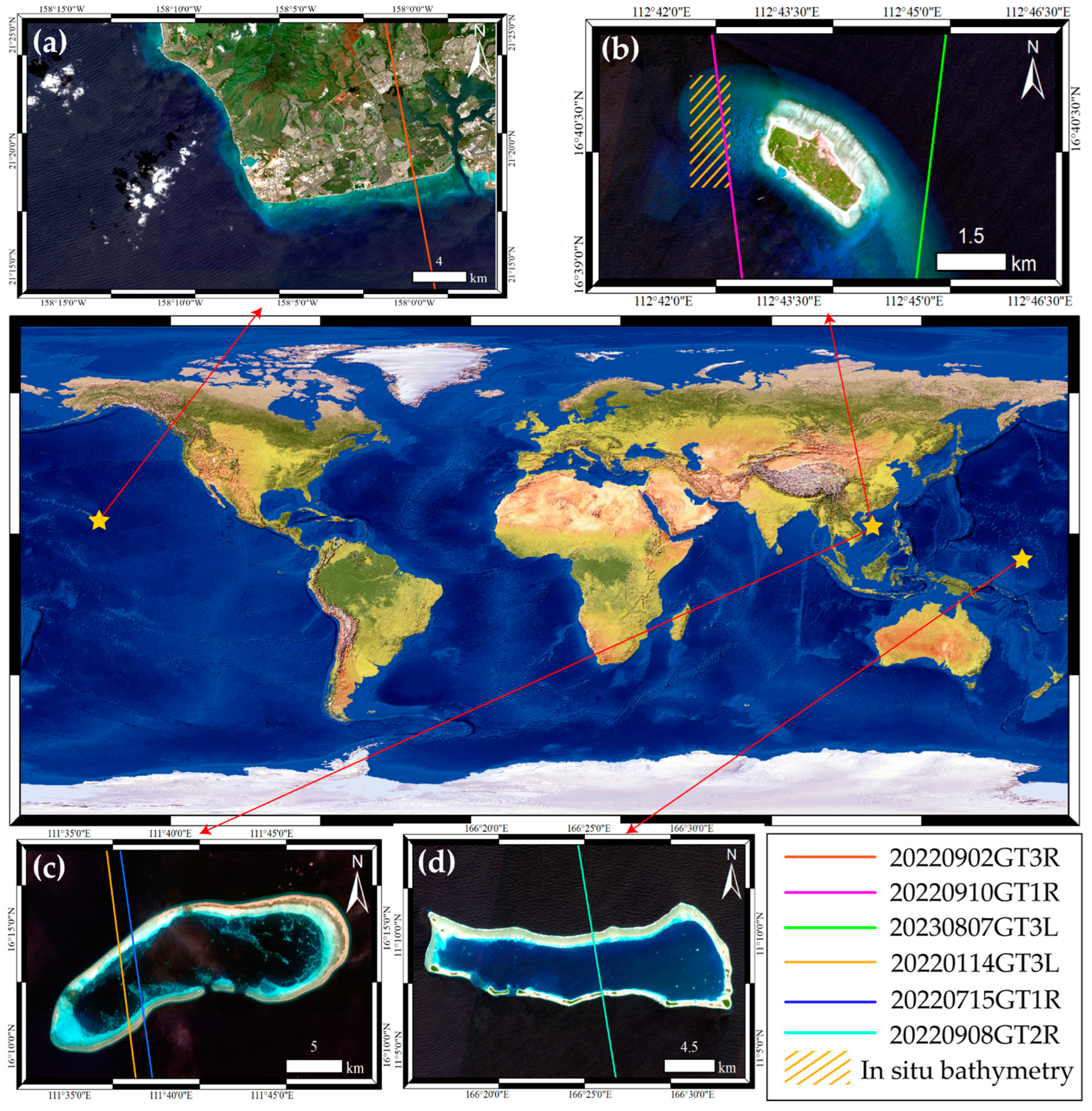
Figure 1.
Distribution of Experimental Areas. (a) Oahu Island; (b) Dongdao Island; (c) Huaguang Reef; (d) Ailinginae Atoll. The solid lines in each study area represent the flight trajectory of ICESat-2, and the yellow diagonal lines in (b) represent the in situ depth measurement data.
2.2.2. Reference Datasets of ICESat-2 by Visual Interpretation
To ensure the accuracy of the experimental results, an accuracy verification strategy based on visual interpretation and in situ bathymetry data was employed. This section focuses on the strategy involving visual interpretation.
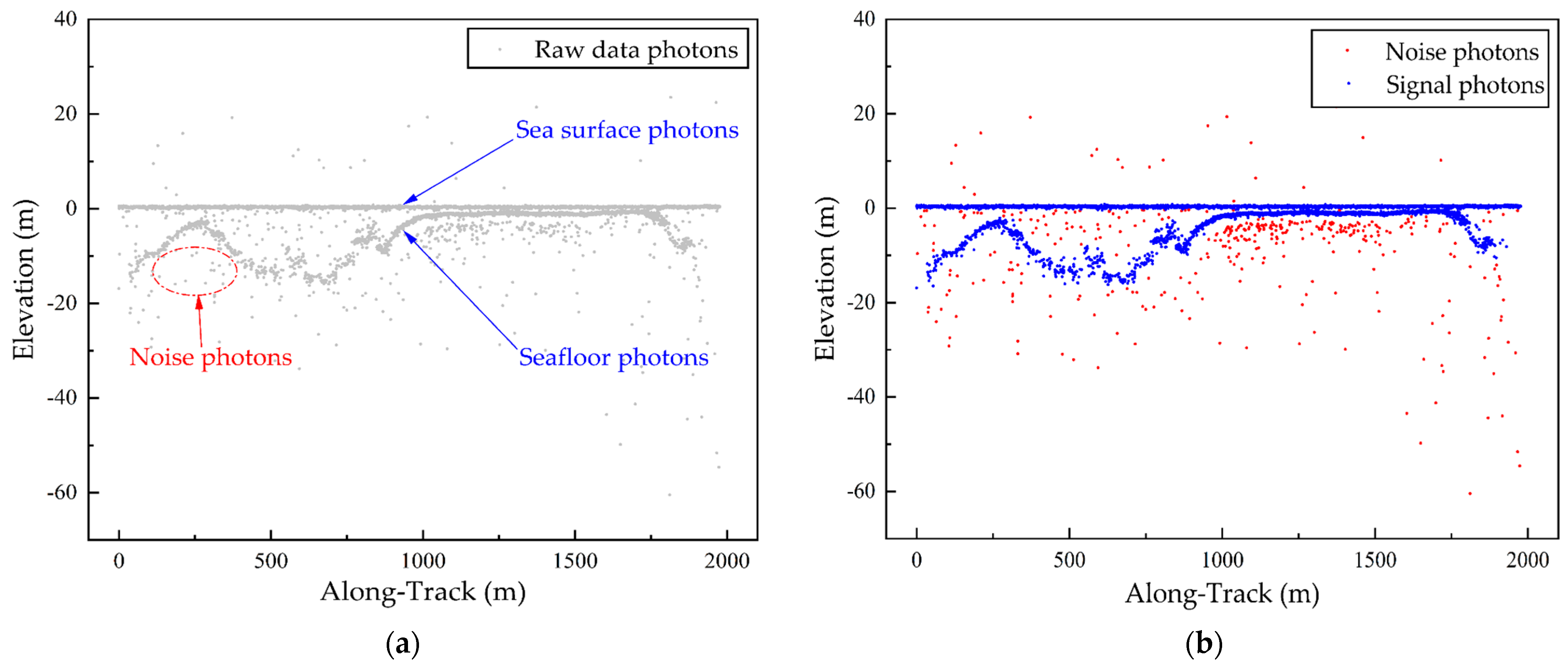
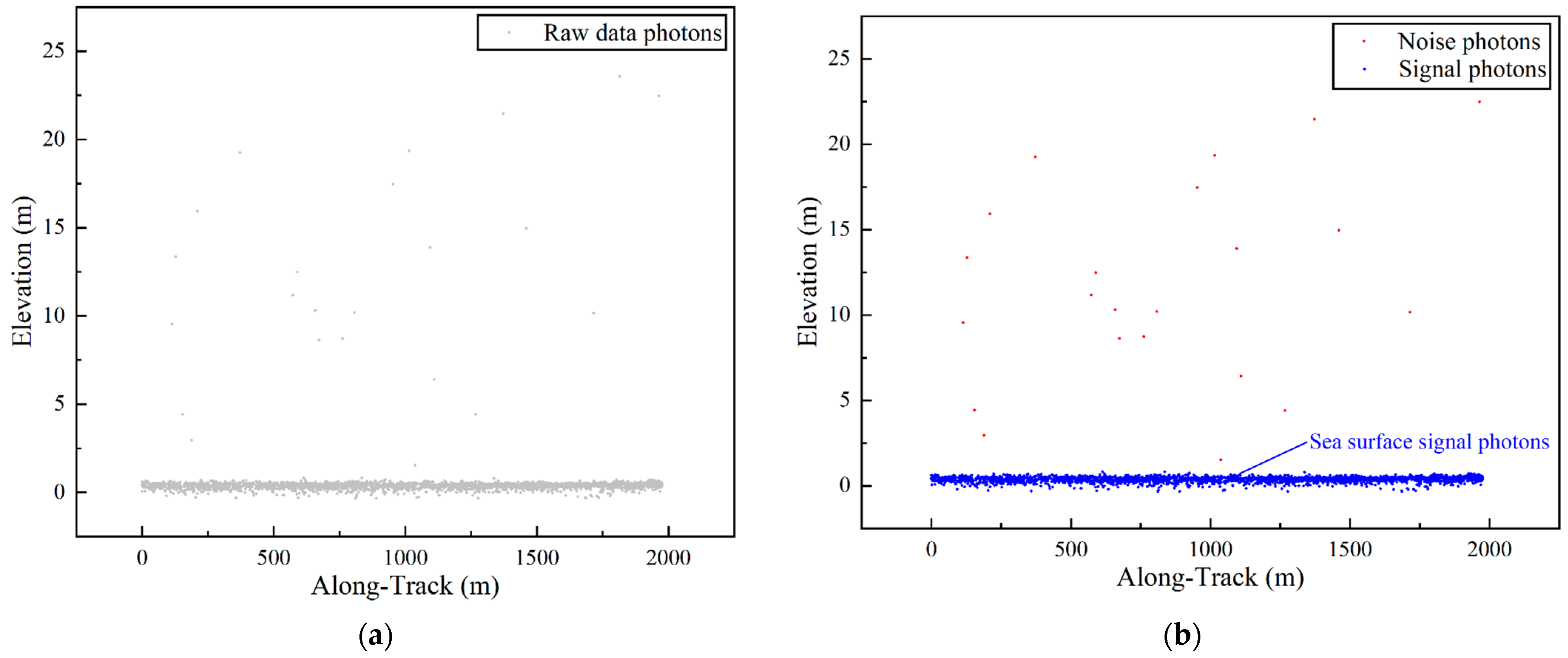
As some of the photon cloud data lack direct validation results, manually annotated photon cloud classification data were predominantly used for validation. In the original data, two distinct density clues were identified (as shown in Figure 2a). It has been demonstrated in many studies that these two lines represent sea surface photons and seafloor photons, respectively, while other scattered photons are noise [7,24,30,31,32,33,34,35,36]. The photon cloud data were imported into specialized software, where photons were manually annotated and classified into noise photons (marked with red) and signal photons (marked with blue). All annotated photon data from the experimental areas were used as the validation dataset. Ensuring the integrity and continuity of these two lines allows for the extracted reference data to be effectively used as the validation dataset [17,37]. Additionally, to minimize the impact of subjectivity in data extraction, high-confidence photons from ICESat-2 (confidence = 4) were used as the benchmark for the reference data. Following this strategy, the ICESat-2 signal photons extracted through visual interpretation formed a reference dataset consisting of six tracks. Figure 2b displays the classification results for the Huaguang Reef.
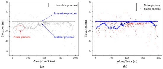
Figure 2.
ATL03 raw data points distribution and reference data. (a) Distribution of the ATL03 raw data. (b) Example of the classification results of the reference data.
2.2.3. In Situ Bathymetry Data
To further verify the accuracy of the experimental results, this study uses shipborne single-beam echo-sounder system data from the Dongdao Island region as reference data. These data were collected in 2012 by the First Institute of Oceanography, Ministry of Natural Resources, using a shipborne single-beam echo-sounder system. The measurement error of these in situ bathymetry data is at the centimeter level, and the spatial coverage includes the western region of Dong Island. The detailed spatial distribution is shown in Figure 1b. Because the positions of the signal photons extracted from the field sounding points and ICESat-2 satellite data do not match completely, this study uses the kriging interpolation method to generate 10 m × 10 m grid-measured water depth data for accurate verification. Kriging interpolation is a tool widely used in geospatial analysis that can estimate the value of an unknown location with high accuracy [38]. To ensure the interpolation accuracy, some known data are retained as validation sets for cross-validation. Finally, the coordinates of the ICESat-2 signal photons are used to extract the corresponding grid image pixel values for data comparison [32,34].
2.3. Methods
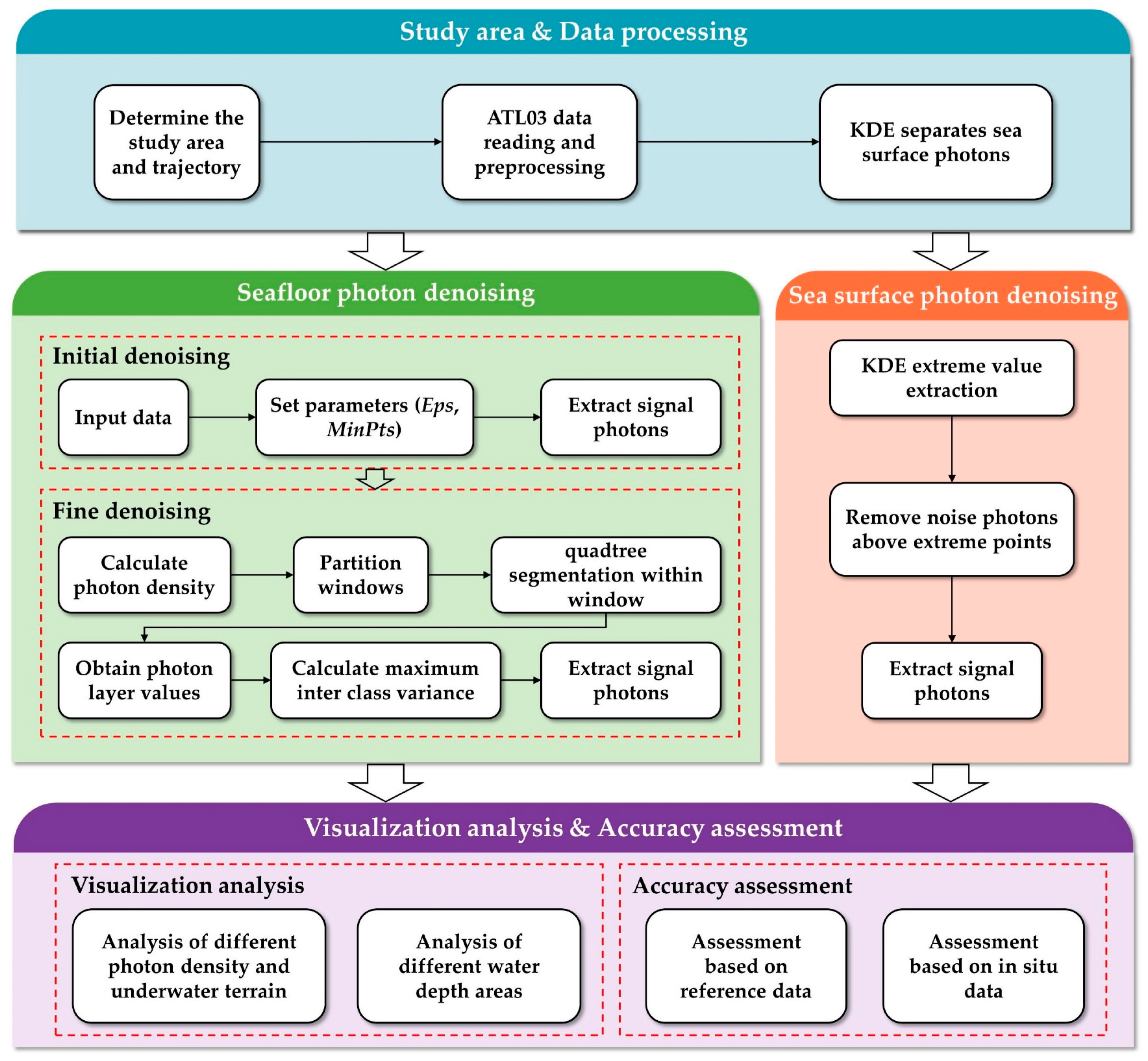
In the photon point cloud collected by ICESat-2, the spatial distribution difference between signal and noise photons is often large, manifested in the denser distribution of signal photons than noise photons [39,40]. This difference in density is the fundamental basis for current ICESat-2 point cloud denoising; therefore, selecting an appropriate density threshold is the key to correctly extracting signal photons. This paper proposes a denoising algorithm based on quadtree and multiscale analysis (as shown in Figure 3), which mainly includes the following steps: (1) study area and data processing, (2) seafloor photon denoising, (3) sea surface photon denoising, and (4) visualization analysis and accuracy assessment.
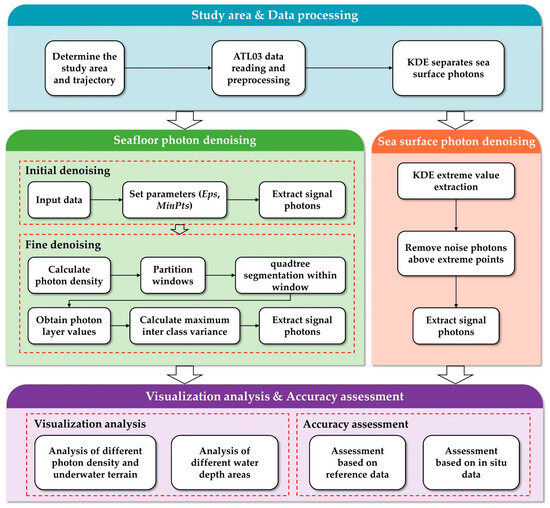
Figure 3.
Method flow chart.
2.3.1. Sea Surface Photon Point Extraction
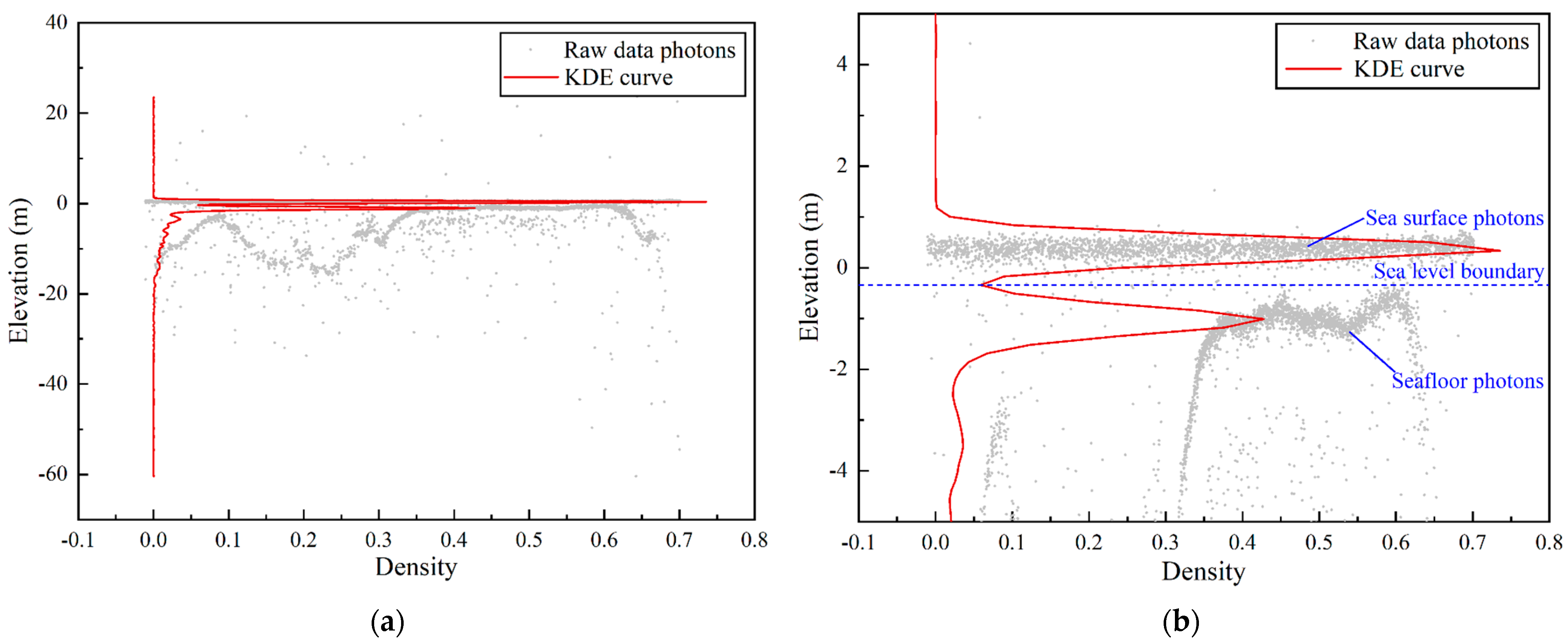
This study uses the KDE method to analyze the photon density distribution along the elevation direction in ICESat-2 satellite data [41,42]. The elevation histogram method is a common way to solve this problem, but the histogram discretizes point cloud data, making it unable to reflect the differences between neighboring point cloud data, thus affecting the extraction accuracy. As a nonparametric probability density estimation technique, KDE enables us to estimate photon density accurately without presetting the data distribution pattern. The formula for KDE is as follows:
where represents the estimated density at point ; is the total number of sample data points; is the bandwidth, which controls the width of the kernel and directly affects the smoothness of the estimated density; represents a single data sample point; is a kernel function; and the Gaussian kernel function is used in this study.
When processing the ICESat-2 data, this study first calculates the KDE curve of the photon density along the elevation direction. By carefully selecting the bandwidth parameters, we ensure that the curve can smoothly reflect the proper distribution of the photon density. It is essential to select the appropriate bandwidth, which must balance the smoothness of the curve and the retention of data features. This study uses a cross-validation method to determine the optimal bandwidth to effectively achieve this goal.
In the KDE curve analysis, the closest minimum point below the first local maximum of the curve is selected as the boundary threshold between sea surface photons and seafloor photons. This method is based on the following assumptions: the first local maximum of the curve represents the local maximum photon density, which usually corresponds to reflected photons from the sea surface, and the minimum point below the first local maximum marks a significant reduction in photon density, which can be used as the natural boundary between reflected photons from the sea surface and photons scattered from the water. Based on this, photons are divided into two categories: photons located above the minimum point are classified as sea surface photons; and photons below the minimum point are identified as seafloor photons (as shown in Figure 4).
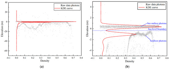
Figure 4.
Extraction of sea surface photon points. (a) The overall KDE curve. (b) The photon extraction details.
For the extracted sea surface photons (as shown in Figure 5a), the threshold can be directly set to extract signal photons. Because the noise points above the sea surface are sparse, the closest minimum point above the first local maximum of the curve is usually selected as the threshold value to eliminate the noise points. The denoising results are shown in Figure 5b.

Figure 5.
Sea surface photons. (a) The distribution of the sea surface photons. (b) The extraction of the sea surface signal photons.
2.3.2. Initial Denoising
The ATLAS laser on the ICESat-2 satellite mainly emits and receives weak signals, which leads to many mixed signal photons and noise photons. However, the spatial distribution of signal photons is denser than that of noise photons. Using the discrete characteristics of signal and noise photons in spatial distribution, we can use the DBSCAN algorithm to eliminate outliers effectively. This method uses the spatial density difference to identify and eliminate noise photons to improve the accuracy and availability of the data.
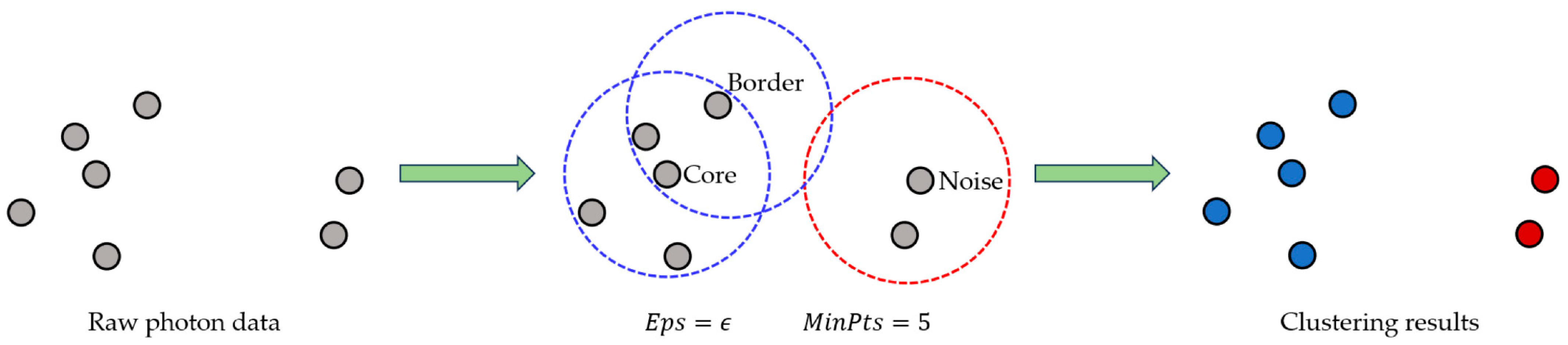
The DBSCAN algorithm, which is a density-based clustering algorithm, was proposed by Martin Ester in 1996 [18]. This algorithm distinguishes signal points from noise points by identifying and connecting points with similar densities (i.e., clusters). The advantage of the DBSCAN algorithm lies in its simplicity and computational efficiency. It mainly depends on two parameters, EPS and MinPts. When the number of points within the specified neighborhood radius exceeds the set minimum number threshold, the point is considered a signal point. This method is especially suitable for processing datasets with complex spatial distributions and can effectively separate signal points and noise points. Figure 6 is a schematic diagram of the DBSCAN clustering principle.
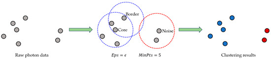
Figure 6.
DBSCABN clustering principle. The blue circles represent the signal photons, and the red circle represents the noise photons.
Given the number of sample points contained in the calculation set of function , if the following formula is met, the sample is called the core point.
where is the circular radius centered on the sample . If is the core point, is the minimum number of points that must be included in .
The DBSCAN algorithm defines density core points, boundary points, and noise points through the density parameters set by users. It regards the dense area formed by density core points and boundary points within the same distance parameter range as a cluster. Research shows that the DBSCAN algorithm is sensitive to manually set parameters, and its effect may not be satisfactory when dealing with datasets with uneven density distributions or unclear clustering boundaries. However, the algorithm performs well with small terrain changes and short regional distances. Based on these considerations, this study uses the DBSCAN algorithm to remove some abnormal noise points.
2.3.3. Fine Denoising
For ICESat-2 raw data, some outliers can be effectively removed after DBSCAN rough denoising, but there are still many dense noise points around the signal points that cannot be removed. Therefore, this study first divides the underwater photon point cloud into windows and then performs quadtree denoising on the photon point cloud in the window to achieve the best denoising effect.
Because the density and distribution of photon point clouds in different experimental areas are different, if quadtree segmentation is directly carried out inside the window, the photon layer value will be high, the density segmentation threshold will be too large, and some signal photons will be misjudged as noise. Therefore, according to the quadtree segmentation algorithm and the distribution characteristics of underwater photon point clouds, this paper proposes a strategy of first dividing the underwater photon window and then performing quadtree denoising. The window is divided according to the 100 photons/window rule along the elevation direction. When there are fewer than 100 photons in the window, the window is divided directly. The number of windows divided into different experimental areas is different. After the division, the windows are roughly dense in shallow places and sparse in deep places. Follow-up experiments are carried out in the divided windows.
The quadtree method is used to separate photons, characterizing photon density using photon layer values. Specifically, the space is recursively divided into four quadrants based on the position of photons in the two-dimensional ‘elevation’ (m) and ‘along-track’ (m) space [43], and the photon density is quantified according to the layer value of the quadrant leaf node of the quadtree where the photons are finally located. The partition process starts with setting an initial root node space and the number of photons in the record. When the set maximum space photon accommodation value is exceeded, the current space is divided into four identical sub-quadrant spaces: upper right (I); upper left (II); lower left (III); and lower right (IV). The number of photons in each subspace is calculated. The number of photons in each subspace is calculated. For subspaces that exceed the limit , further division is performed, and partitioning is recursively executed until the number of photons in each subspace is within the limit . At this point, photons are located in the partitioned spaces corresponding to each leaf node. The quadtree partition criteria can be summarized as follows:
where is the set of quadrants that can be divided into layer ; is the quadrant set of layer ; is a quadrant space in , and is the number of photons in quadrant space . To ensure the denoising degree, it is usually necessary to separate each photon; thus, is generally set to 1. The quadtree flowchart is shown in Figure 7.
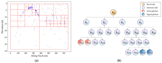
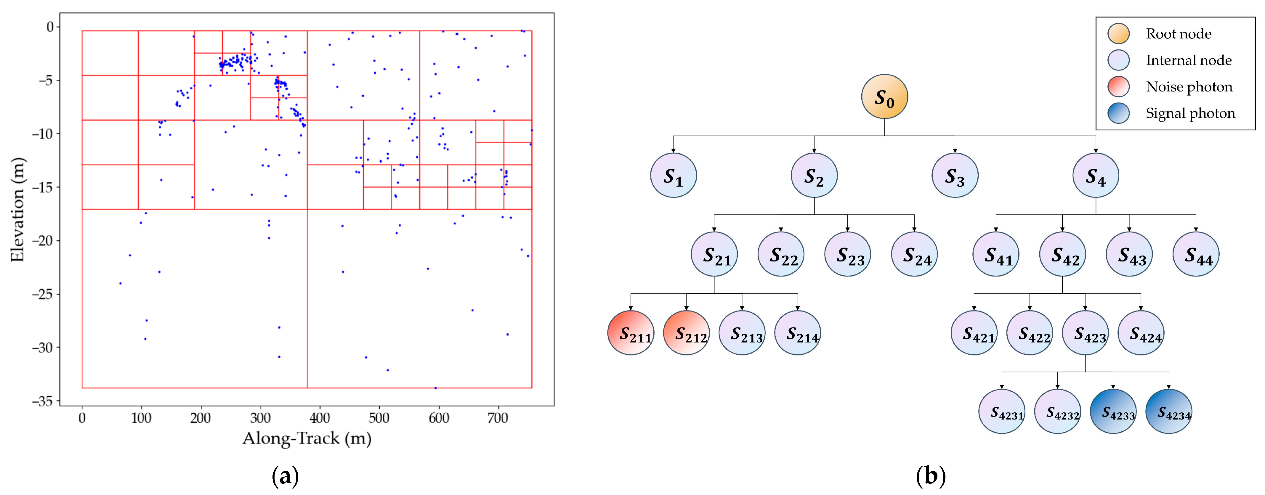
Figure 7.
Quadtree flowchart. (a) The quadtree segmentation process, with four segmentation layers and a maximum spatial photon capacity of 20. (b) The quadtree structure.
The distribution of noise photons usually exhibits randomness. In some local sparse regions, noise photons may be close to each other; therefore, they need more space division, resulting in higher layer values of corresponding photons. In this case, these photons may be mistaken for signal photons in the denoising process. To solve this problem, this study utilizes the pre-judged strategy to optimize the quadtree structure and improve the algorithm’s efficiency by deleting some invalid nodes [25]. The specific pre-judged process involves first analyzing and judging the quadrants to be divided. If no photons are effectively separated after a partition, the partition will not be performed, and further partitioning of the quadrant will also terminate. In this way, the dendritic structure caused by unreasonable partitioning will be cut off. The space division criteria of the pre-judged quadtree are as follows:
where is the number of spaces in which the number of photons in the sub-quadrant space is not less than one after the quadrant space is divided into four levels: the number of sub-quadrant spaces with photons.
After the improvement in the quadtree partition, the partition criterion is no longer based on but considers the distribution of photons in the quadrant space. According to the division criteria, there are two situations for the division of quadrant space :
- If there is no photon or only one photon in a quadrant space, the quadrant will not be divided, and then the division process of the quadrant will terminate;
- For a quadrant space containing multiple photons, the quadrant is first analyzed and judged. If all photons are still in the same quadrant after a quartering division, the division will not be performed, and the division of the quadrant will also be terminated. If photons are distributed in different quadrants, the division will be performed, and the above two cases will continue to be iterated according to the number of photons in the divided sub-quadrants until no further division is needed.
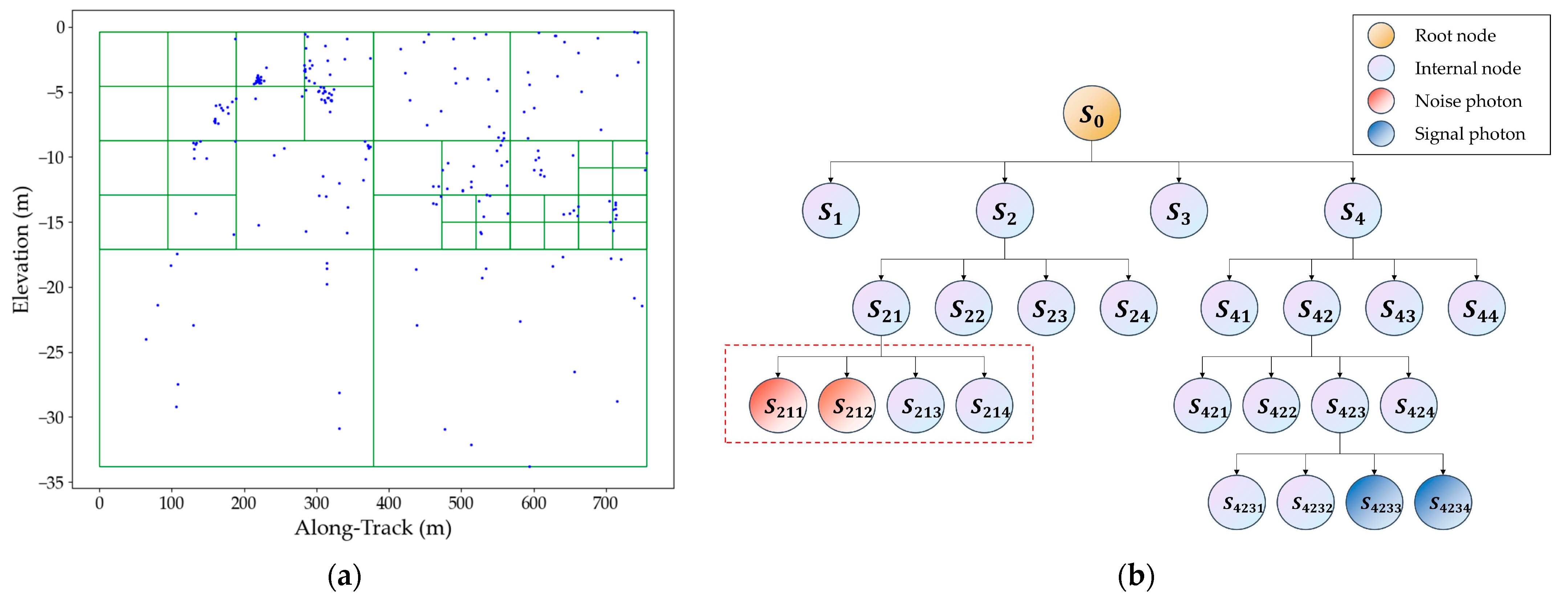
Figure 8a shows the case where the pre-judged quadtree splits some photons. Compared to Figure 7a, the quadrant within the green box in the upper left corner is no longer divided according to the division criteria. The corresponding tree structure in Figure 8b shows that the noise photons within the red dashed box are no longer divided. By introducing the pre-judged strategy, the layer value of noise photons is low, while that of signal photons is high, thus allowing for classification through calculating the segmentation threshold.
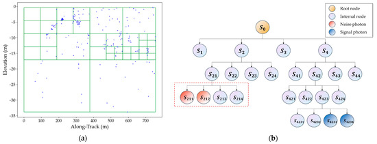
Figure 8.
Optimized quadtree flowchart. (a) The optimized quadtree segmentation process, with four segmentation layers and a maximum spatial photon capacity of 20. (b) The optimized quadtree structure.
Due to the influence of surface reflectivity, solar altitude angle, atmospheric scattering, and other factors, the noise density of photons in different regions along the orbital direction will differ [44]. To adapt to the difference in the density comparison of signal photons and noise photons along the rail direction, 100 m equidistant windows are divided along the rail direction [45]. The density threshold of photons in each window is adaptively calculated by the Otsu method [46], and the noise photons and signal photons are classified according to the density threshold. The Otsu algorithm, also known as the maximum between-class variance method, is a threshold determination algorithm proposed by Japanese scholar Nobuyuki Otsu in 1979 [46]. Suppose that the value range of all photon layer values in a window is , and assuming the density threshold is , the photons in the window are divided into two categories, the layer values are and , and the variance between categories is as follows:
where
where is the proportion of photons with layer value in the window; and are the proportions of photons with layer values less than and greater than or equal to , respectively; and are the average values of photon layer values less than and greater than or equal to , respectively; and is the average value of all photons in the window.
When some noise photons are misclassified as signal photons or some signal photons are misclassified as noise photons, the interclass variance decreases. Therefore, the maximum interclass variance indicates that the probability of misclassification between the two types of photons is at a minimum; therefore, the optimal density threshold of photons in the window is as follows:
That is, is taken from , and is the corresponding value when the interclass variance is maximized. Currently, photons with inner layer values less than in the window are classified as noise photons, and the others are classified as signal photons. According to the classification results, the noise photons are removed to complete the denoising.
2.3.4. Accuracy Evaluation
To verify the advantages of this research method more rigorously, this paper uses the visual interpretation results as the accuracy benchmark. The confusion matrix is constructed to calculate the overall accuracy (OA), precision (P), recall (R), F1 value (F), and false-positive rate (FPR). The OA indicates the proportion of photons correctly classified in the total sample. The P indicates the accuracy of signal photon recognition, which is the proportion of correctly recognized signal photons to the total number of photons identified as signal photons. The R indicates the ability to identify signal photons, which is the proportion of correctly identified signal photons to the total number of actual signal photons. The F indicates the harmonic average of the precision and recall rates, which is used to balance the two indicators, assuming that they are equally important. The FPR represents the proportion of samples that are incorrectly predicted as signal photons in all samples that are not signal photons. The specific equations for these evaluation metrics are as follows:
In the formulas, the photon whose predicted value and actual value are judged as signals at the same time is defined as TP; TN is judged as noise at the same time; FP is defined as the predicted signal but the real noise; and FN is the definition of the predicted noise but the actual signal. Generally, the higher the OA, P, R, and F are, the lower the FPR and the better the denoising effect.
For the quantitative comparison of the reference measured water depth, this paper calculates the determination coefficient (R2), root mean square error (RMSE), mean relative error (MRE), and mean absolute error (MAE), which are defined as follows:
3. Results
To evaluate the effectiveness of the proposed method, the ATL03 built-in algorithm (confidence = 4), DBSCAN denoising results, and quadtree denoising results were compared with the denoising results presented in this paper, and the feasibility and rationality of the proposed method were verified by analyzing the photon density and underwater terrain. This experiment was conducted in Python 3.9 and ran on an Intel Core i7-11800h 2.30 GHz Windows 11 computer.
3.1. Visualization of the Denoising Results
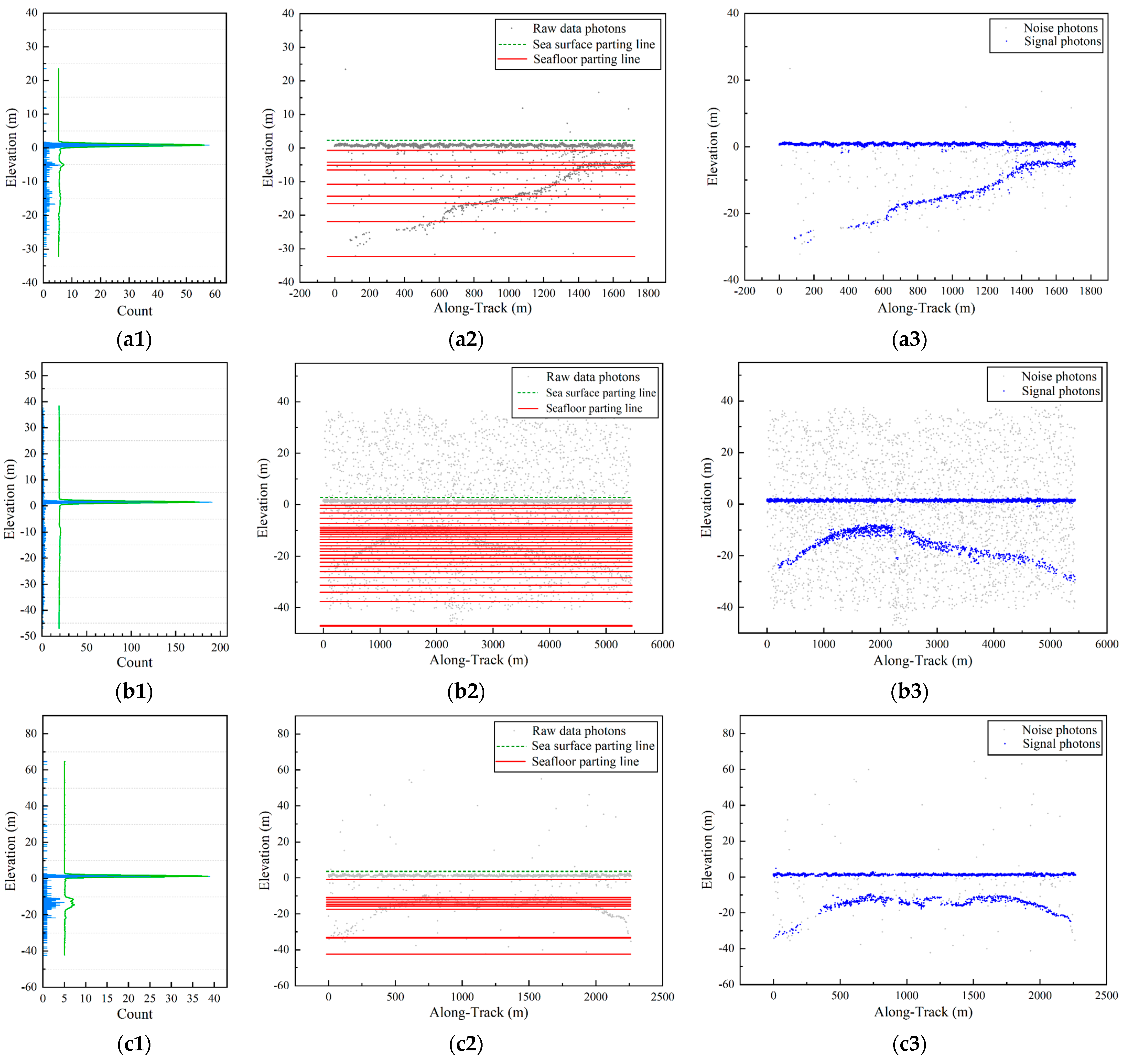
Figure 9 shows the denoising results for each experimental area (Oahu Island, Dongdao Island, Huaguang Reef, and Ailinginae Atoll). The first column depicts the photon density and KDE curve; the second column illustrates details of the multiscale analysis, and the third column demonstrates the denoising results of the method proposed in this paper.
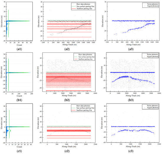
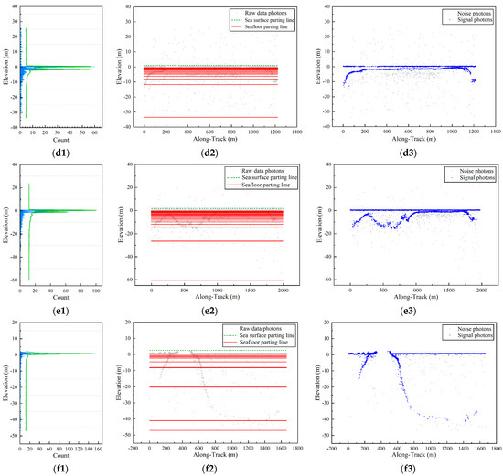
Figure 9.
Experimental results. (a1–a3) Oahu Island; (b1–b3) Dongdao Island in 10 September 2022; (c1–c3) Dongdao Island in 7 August 2023; (d1–d3) Huaguang Reef in 14 January 2022; (e1–e3) Huaguang Reef in 15 July 2022; (f1–f3) Ailinginae Atoll Island.
As shown in Figure 9, photon density is highest at the sea surface. As water depth increases, photon density declines gradually. The green dotted line depicts the noise extraction threshold above the sea surface, while the red solid line denotes the segmentation value for the underwater window. The window distribution exhibits a trend of being dense in shallow areas and sparse in deeper areas. Experimental results demonstrate that the proposed method can effectively remove noise photons in the experimental area and accurately capture the precise contours of the underwater terrain. However, in deeper water, due to the sparse number and distribution of photons, some photons remain unidentified as signal points and are filtered out.
The experimental results further confirm that the proposed method can accurately remove most noise photons. The influence of different terrains on noise removal is minimal, as the quadtree isolation denoising process is segmented only in two-dimensional space and is related only to photon distribution, independent of water depth. Moreover, the denoising results for daytime data are less effective than nighttime data due to the influence of surface reflectivity, solar altitude angle, atmospheric scattering, and other factors, resulting in more noise and affecting the denoising effect.
3.2. Multiple Analysis Strategies for Denoising Results
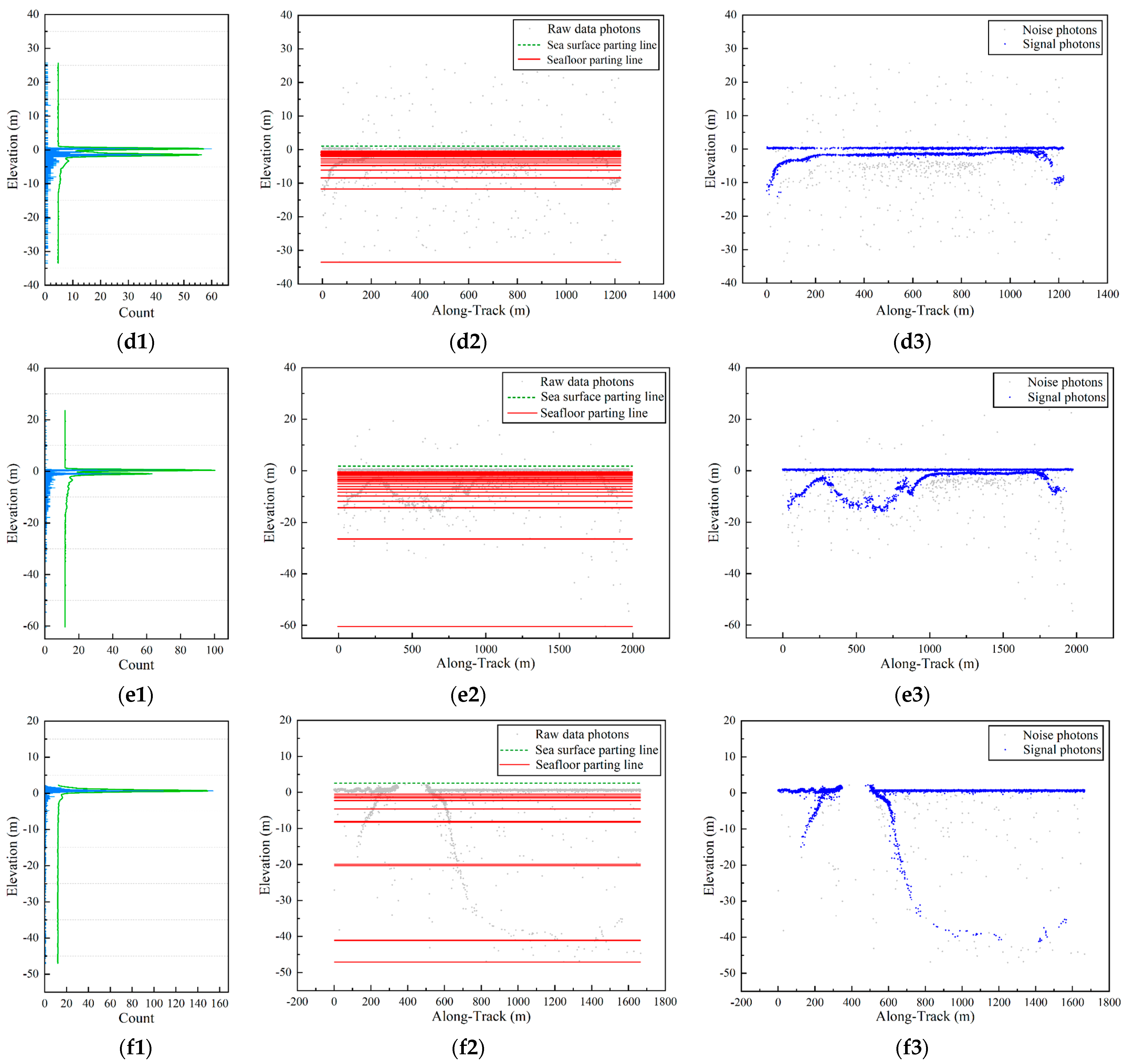
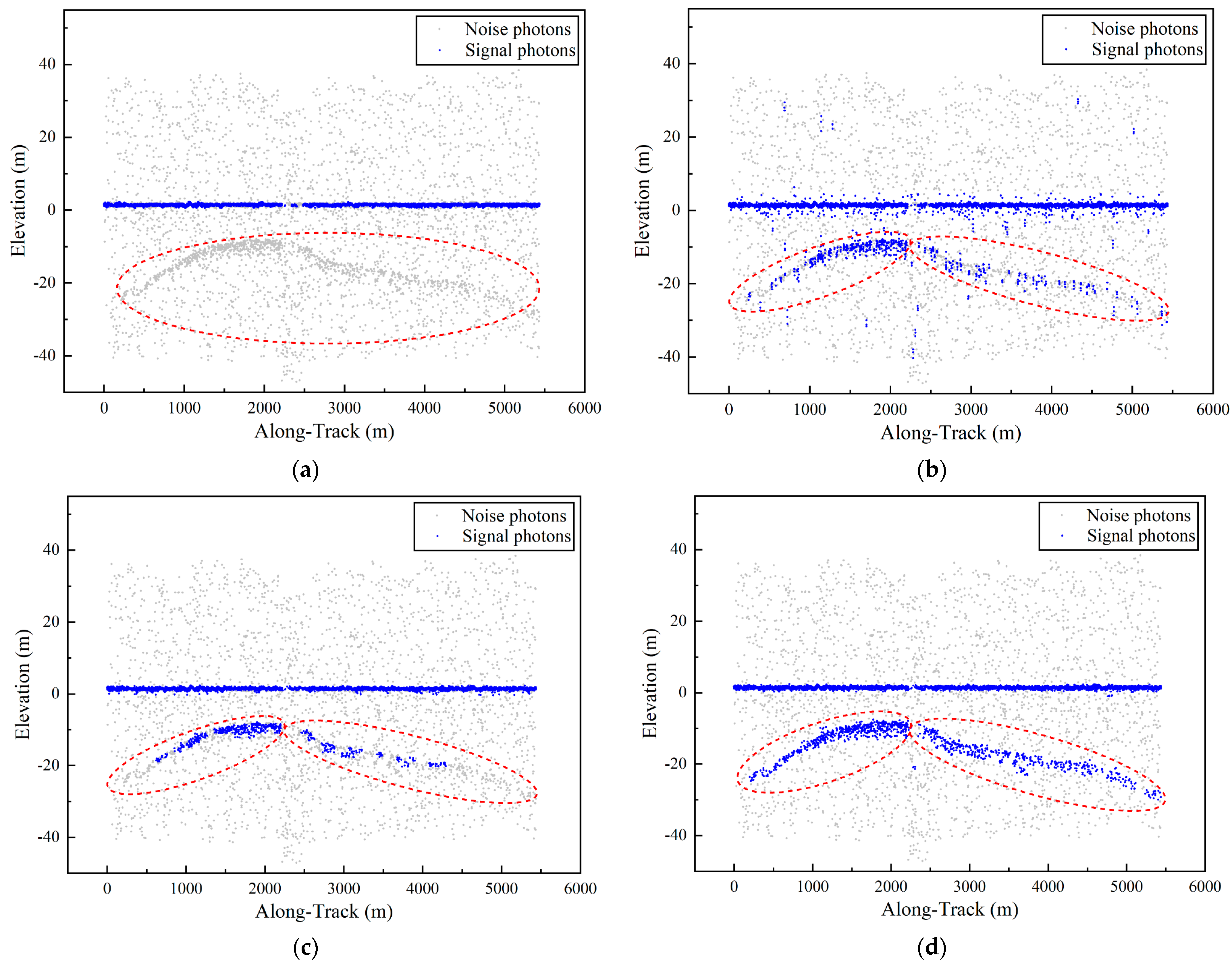
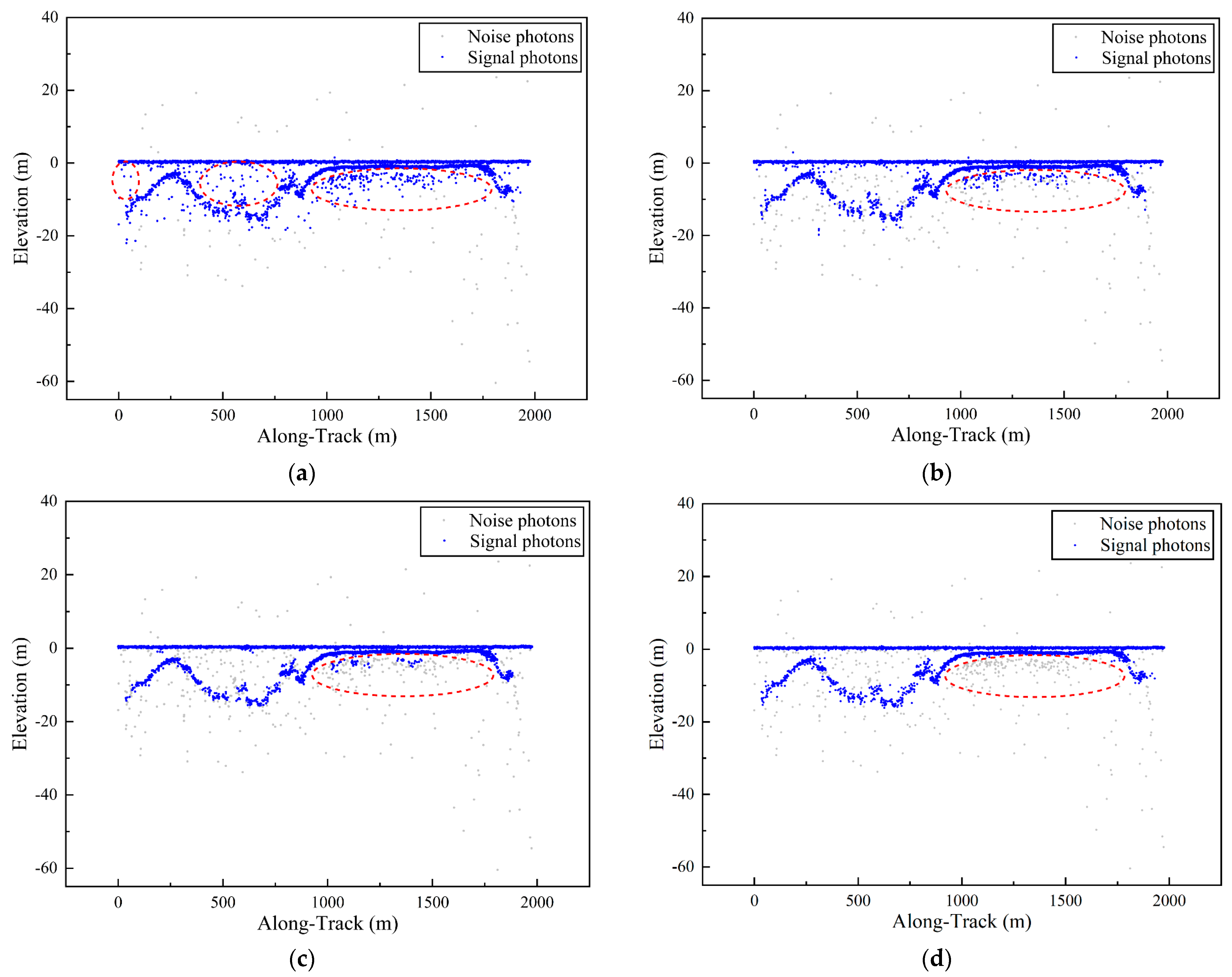
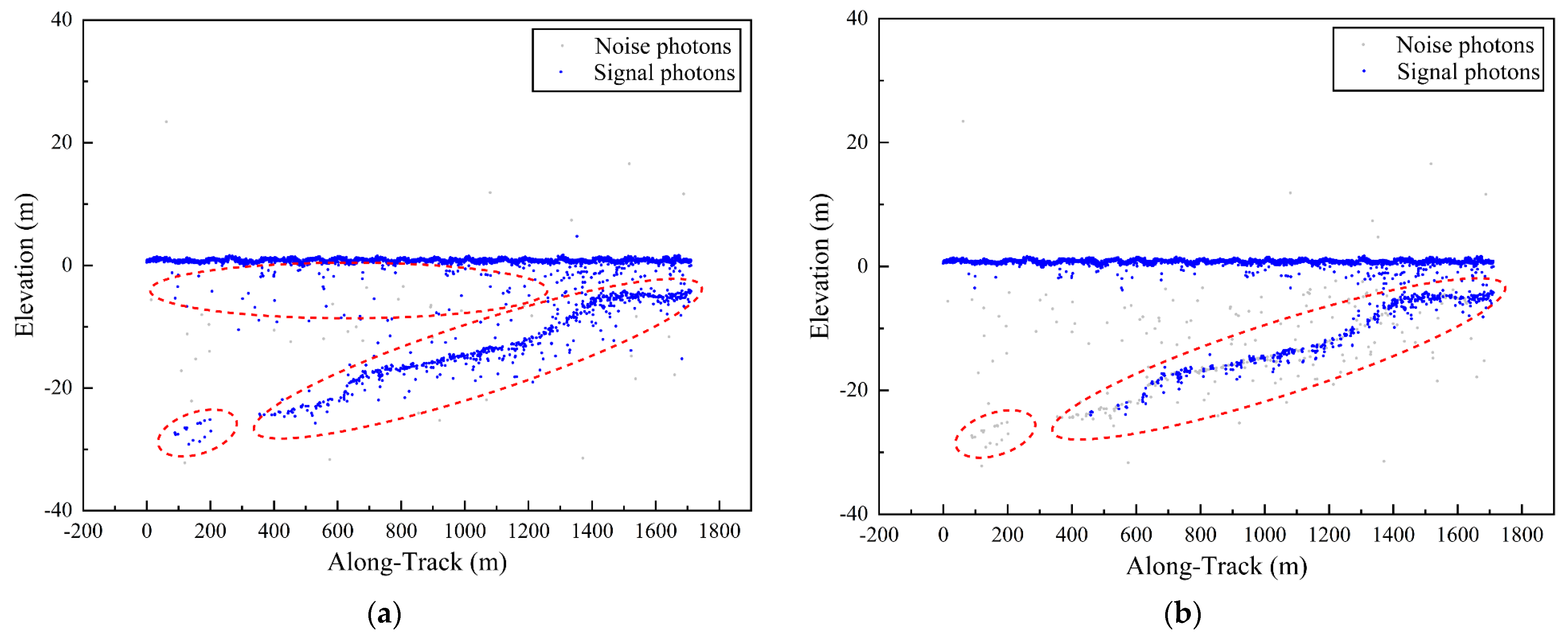
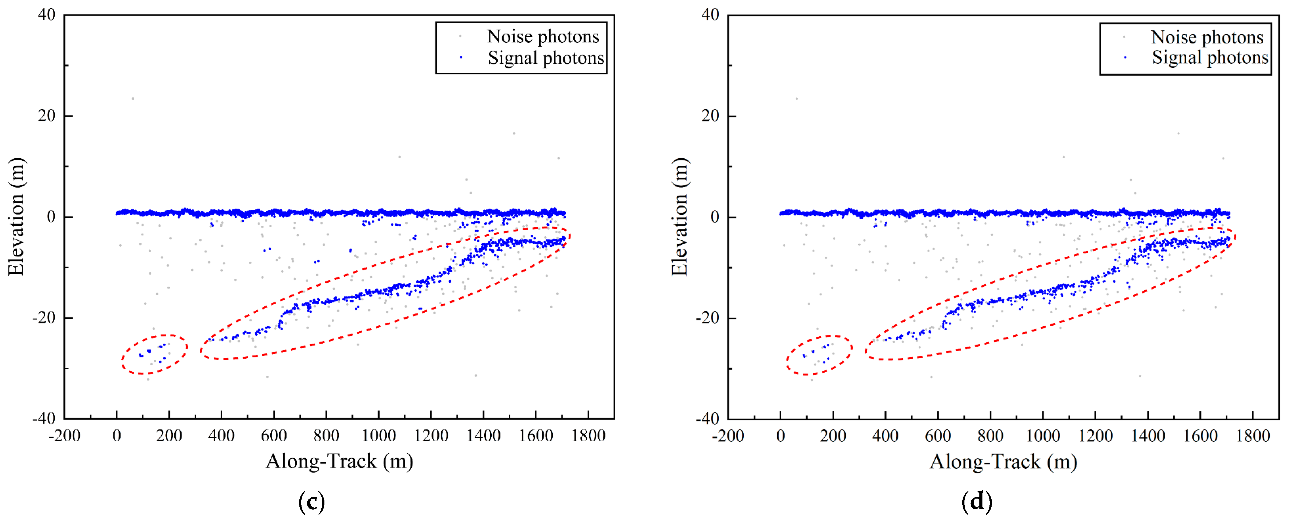
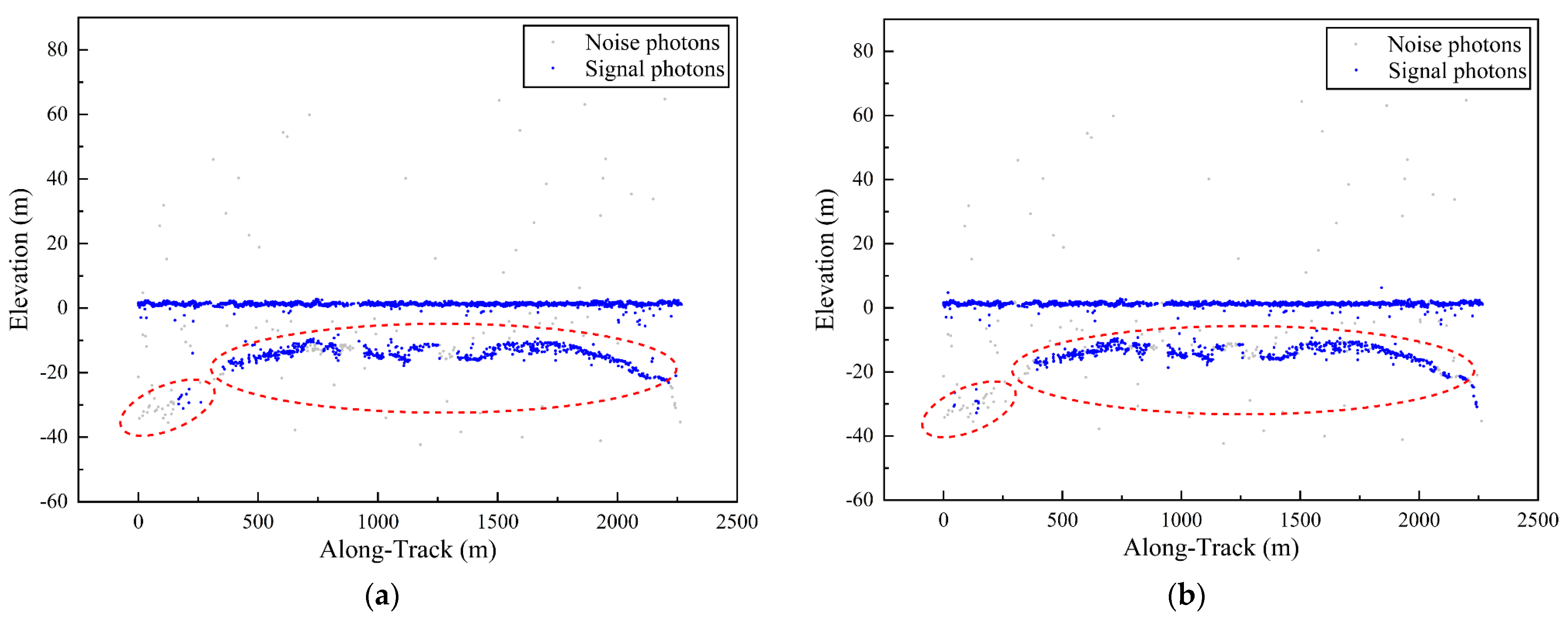
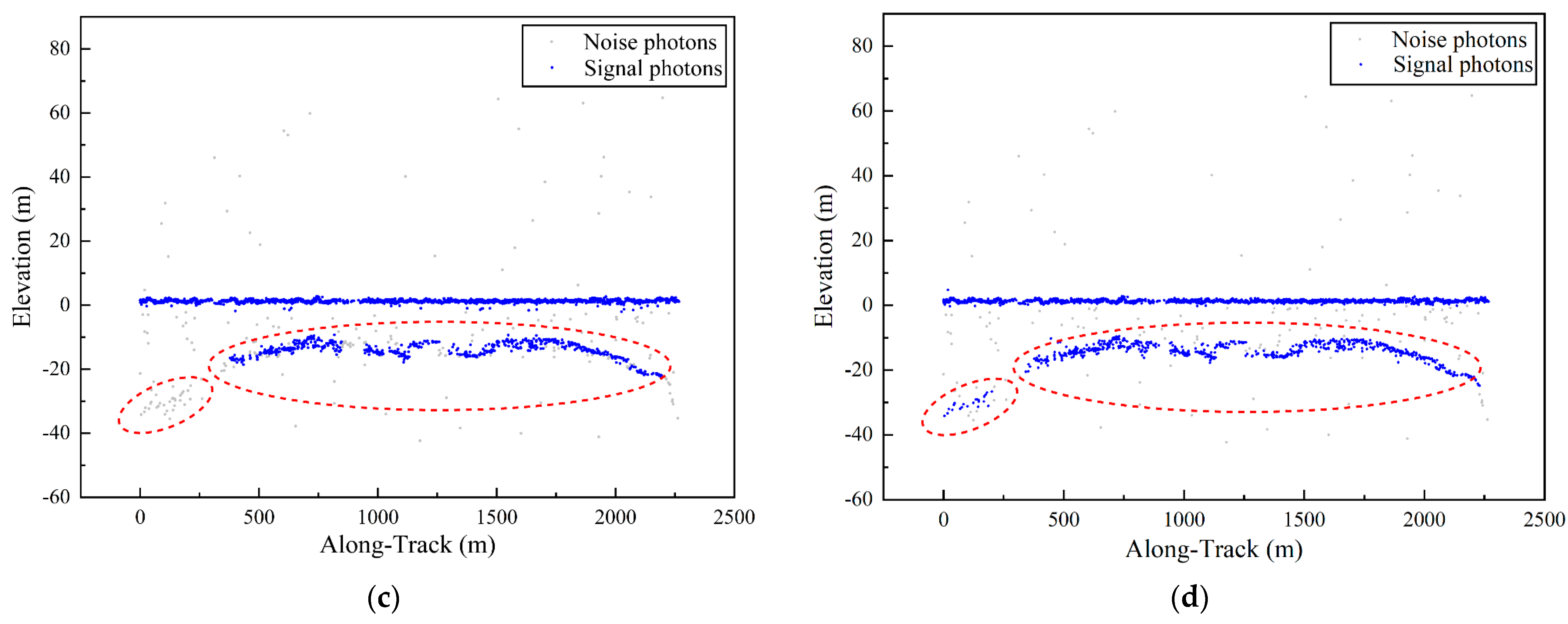
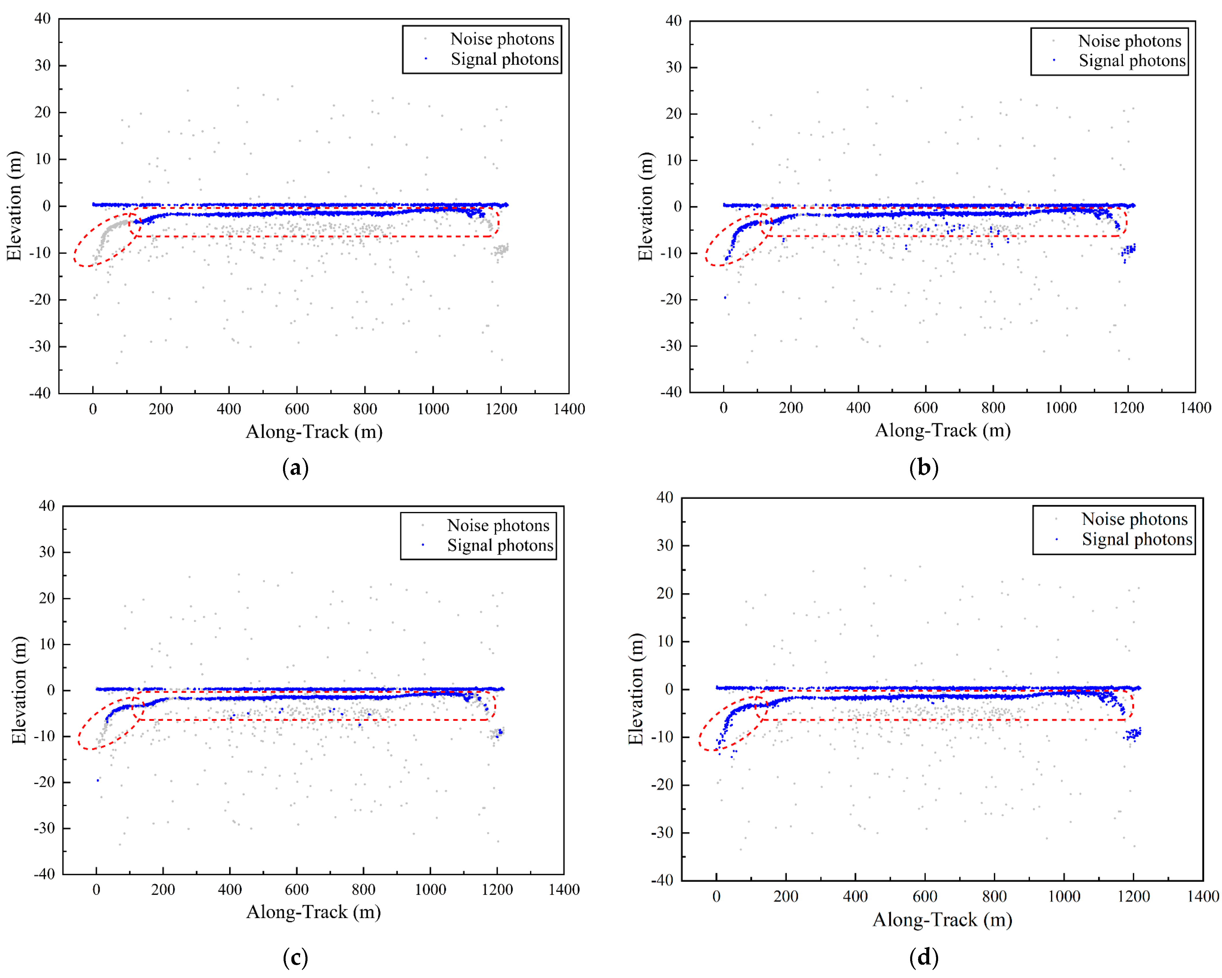
To verify the effectiveness and validity of the proposed method, the denoising results of the ATL03 built-in algorithm (confidence = 4), the DBSCAN denoising algorithm, and the quadtree denoising algorithm were compared. The experimental results are shown in Figure 10, Figure 11, Figure 12, Figure 13, Figure 14 and Figure 15. Since the denoising results are affected by noise density and underwater topography, these two aspects are analyzed and discussed in Section 3.2.1 and Section 3.2.2.
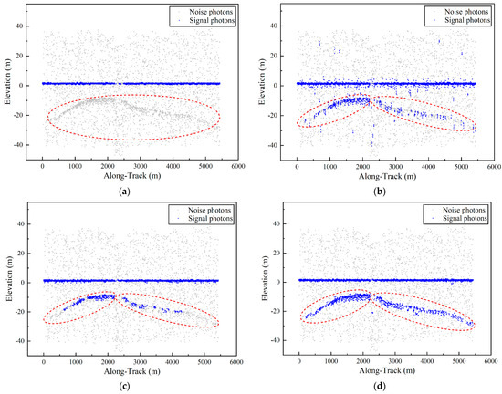
Figure 10.
Comparison of Dongdao Island denoising results in 10 September 2022. (a) ATL03 results. (b) DBSCAN results. (c) Quadtree results. (d) Results of the proposed method.
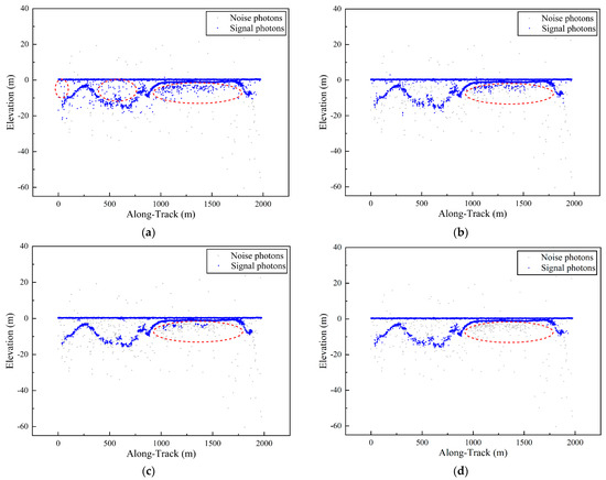
Figure 11.
Comparison of Huaguang Reef denoising results in 15 July 2022. (a) ATL03 results. (b) DBSCAN results. (c) Quadtree results. (d) Results of the proposed method.
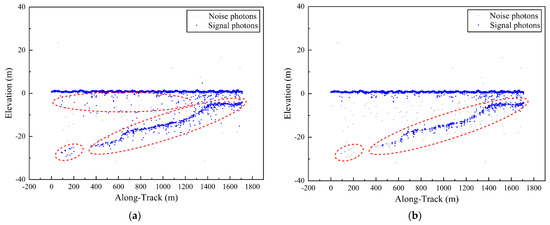
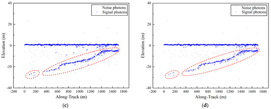
Figure 12.
Comparison of Oahu Island denoising results. (a) ATL03 results. (b) DBSCAN results. (c) Quadtree results. (d) Results of the proposed method.
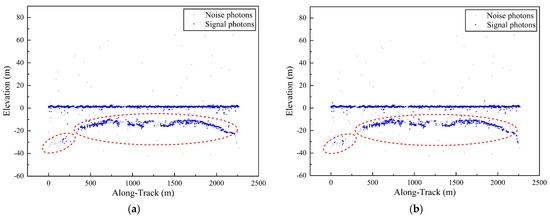
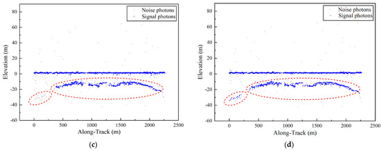
Figure 13.
Comparison of Dongdao Island denoising results in 7 August 2023. (a) ATL03 results. (b) DBSCAN results. (c) Quadtree results. (d) Results of the proposed method.
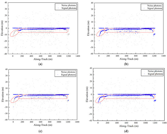
Figure 14.
Comparison of Huaguang Reef denoising results in 14 January 2022. (a) ATL03 results. (b) DBSCAN results. (c) Quadtree results. (d) Results of the proposed method.
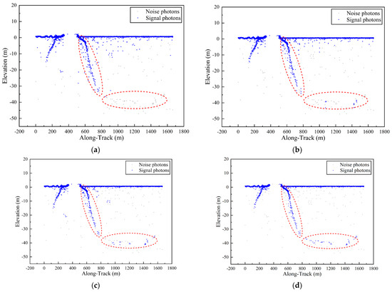
Figure 15.
Comparison of Huaguang Reef denoising results. (a) ATL03 results. (b) DBSCAN results. (c) Quadtree results. (d) Results of the proposed method.
3.2.1. Comparative Experiment Based on the Photon Density Difference
Since the denoising results are affected by noise density, the ATL03 built-in algorithm (confidence = 4), DBSCAN denoising algorithm, and quadtree denoising algorithm were applied in the experimental areas (Dongdao Island, Huaguang Reef, and Oahu Island) for qualitative and quantitative analyses. The effectiveness and universality of the proposed method were validated by comparing the denoising results across different photon density data. As shown in Figure 10, Dongdao Island has a high number of photons and dense noise points. The ATL03 built-in algorithm (confidence = 4) identifies only surface photons, while the DBSCAN and quadtree denoising algorithms exhibit poor denoising performance. In contrast, the proposed method removes noise points and extracts underwater terrain information. Figure 11 demonstrates that the ATL03 built-in algorithm has poor denoising performance. Additionally, the DBSCAN and quadtree denoising algorithms cannot remove noise points near the underwater terrain. In contrast, the proposed method effectively removes noise points in this area and retains valid terrain information. Figure 12 indicates that the noise points on Oahu Island are scattered. Near the sea surface, the ATL03 built-in algorithm (confidence = 4), the DBSCAN denoising algorithm, and the quadtree denoising algorithm fail to completely remove these noise points. In contrast, the proposed method effectively removes the noise points in this area. Additionally, the proposed method can identify signal points in the deep-water area within the red dotted line box.
The experimental results show that the ATL03 built-in algorithm (confidence = 4) and DBSCAN denoising algorithm can extract signal point information for areas with high noise point density but retain numerous noise points post-denoising. In quadtree segmentation of the entire region, the layer value corresponding to photons is high; the maximum interclass variance calculated by the Otsu algorithm is significant, and some signal points with low layer values are misjudged as noise points, resulting in excessive denoising. Compared with the other three denoising algorithms, the method proposed in this paper yields better visual results, effectively removing most noise photons and preserving the contour of the seafloor signal photons.
The denoising results for the experimental areas (Dongdao Island, Huaguang Reef, and Oahu Island) were obtained using visual interpretation data as reference data. The accuracy was evaluated using the following five indicators: OA; P; R; F; and FPR. The accuracy evaluation results are shown in Table 2, Table 3 and Table 4. The experimental results show that the proposed method outperforms the other three algorithms in terms of accuracy for different experimental methods. The R values of the proposed method for Huaguang Reef and Oahu Island are slightly lower than those of the other three denoising algorithms. This occurs because models with low performance often need to sacrifice many P-values to improve the R-value, leading to higher F-value and OA-value compared to the other three denoising algorithms.
Table 2.
Dongdao Island accuracy verification results in 10 September 2022.
Table 3.
Huaguang Reef accuracy verification results in 15 July 2022.
Table 4.
Oahu Island accuracy verification results.
3.2.2. Comparative Experiments Based on Different Terrain Features
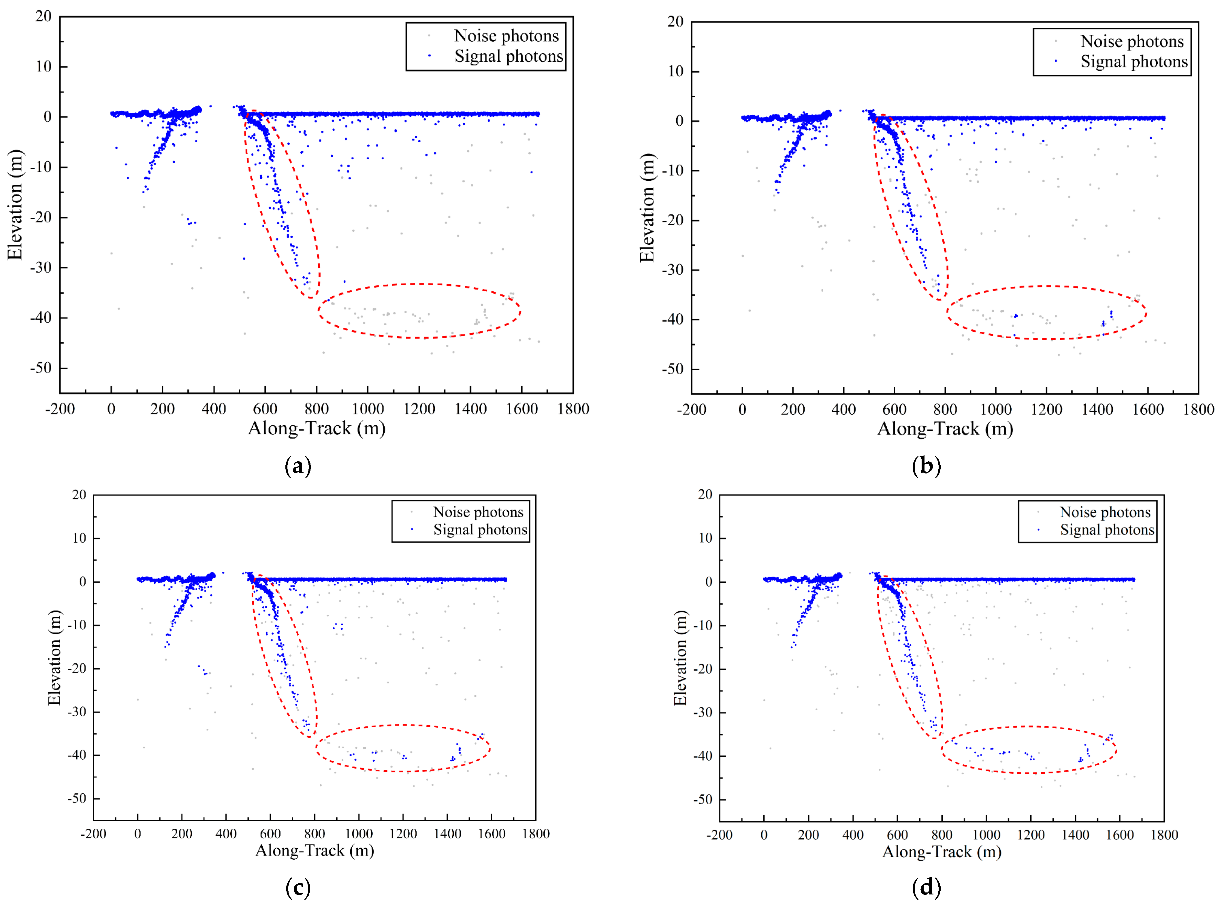
Considering that the denoising results are affected by terrain information, the ATL03 built-in algorithm (confidence = 4), DBSCAN denoising algorithm, and quadtree denoising algorithm were applied in the experimental areas (Dongdao Island, Huaguang Reef, and Ailinginae Atoll) for qualitative and quantitative analyses with the method proposed in this paper. The effectiveness and universality of the proposed method were further verified by comparing the denoising results for different underwater terrain data.
As shown in Figure 13, the underwater topography of Dongdao Island is complex, with scattered noise points. The denoising results of the other three algorithms retain numerous noise points, whereas the proposed method eliminates the noise points within the red dotted box. As shown in Figure 14, the underlying terrain of Huaguang Reef is complex. The ATL03 built-in algorithm and the DBSCAN denoising algorithm retain numerous noise points. Additionally, the quadtree denoising algorithm generates discontinuous underwater terrain information and incorporates some noise. In contrast, the proposed method effectively removes noise points in this area and preserves continuous and smooth underwater terrain information. As shown in Figure 15, the terrain of the Ailinginae Atoll area fluctuates significantly. The other three denoising algorithms fail to eliminate the noise points near the sea surface, and the terrain information in the right dotted box is misidentified as noise. In contrast, the proposed method effectively removes the noise points near the sea surface and identifies the signal points within the red-dotted box.
The experimental results show that the complexity of terrain also has a particular impact on the extraction of signal photons. The ATL03 built-in algorithm and DBSCAN algorithm exhibit poor denoising effects, especially when the noise points near the sea surface cannot be completely removed. The quadtree algorithm removes more noise points, but for the whole region, quadtree segmentation leads to excessive denoising of photon data and discontinuous underwater terrain information. Compared with those of the other three denoising algorithms, the denoising results presented in this paper exhibit superior visual quality, effectively removing noise photons and preserving the details of the underwater terrain.
The denoising results for the experimental areas (Dongdao Island, Huaguang Reef, and Ailinginae Atoll) were derived using visual interpretation data, with accuracy evaluation results shown in Table 5, Table 6 and Table 7. The experimental results show that the proposed method outperforms the other three algorithms in terms of accuracy indices across different experimental areas. For Dongdao Island and Ailinginae Atoll, the precision indices of the proposed method were higher than those of the other three algorithms. For Huaguang Reef, the ATL03 built-in algorithm exhibited lower FPR values. This is because the algorithm misidentified fewer noise points as signal points.
Table 5.
Dongdao Island accuracy verification results in 7 August 2023.
Table 6.
Huaguang Reef accuracy verification results in 14 January 2022.
Table 7.
Ailinginae Atoll accuracy verification results.
3.3. Accuracy Assessment Based on In Situ Bathymetry Data
To further verify the accuracy of the method proposed in this paper, in situ measured water depth data near Dongdao Island and ICESat-2 bathymetry data (i.e., 20230807GT3L) were utilized for correlation analysis. Figure 16 and Table 8 show the regression line slope, R2, RMSE, MAE, MRE, and other information.
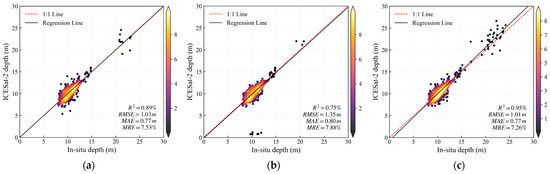
Figure 16.
Scatterplots of ICESat-2 extracted depth and in situ depth for different algorithms. (a) DBSCAN; (b) Quadtree; (c) The proposed method.
Table 8.
Accuracy and validation of photon-counting bathymetry.
Experiments show that the R2 values are both higher than those of the DBSCAN and quadtree denoising algorithms, reaching 94.59%. The results show that the ICESat-2 sounding data after refractive index correction obtained by this method strongly correlate with the in situ sounding data. In addition, Figure 16 and Table 8 illustrate that the ICESat-2 sounding data extracted by this method exhibit almost no abnormal values and high accuracy, with an RMSE of 1.01 m and an MAE of 0.77 m. In conclusion, the signal points extracted by this method have fewer errors than the measured data, and the results can provide valuable insights for subsequent underwater topographic maps.
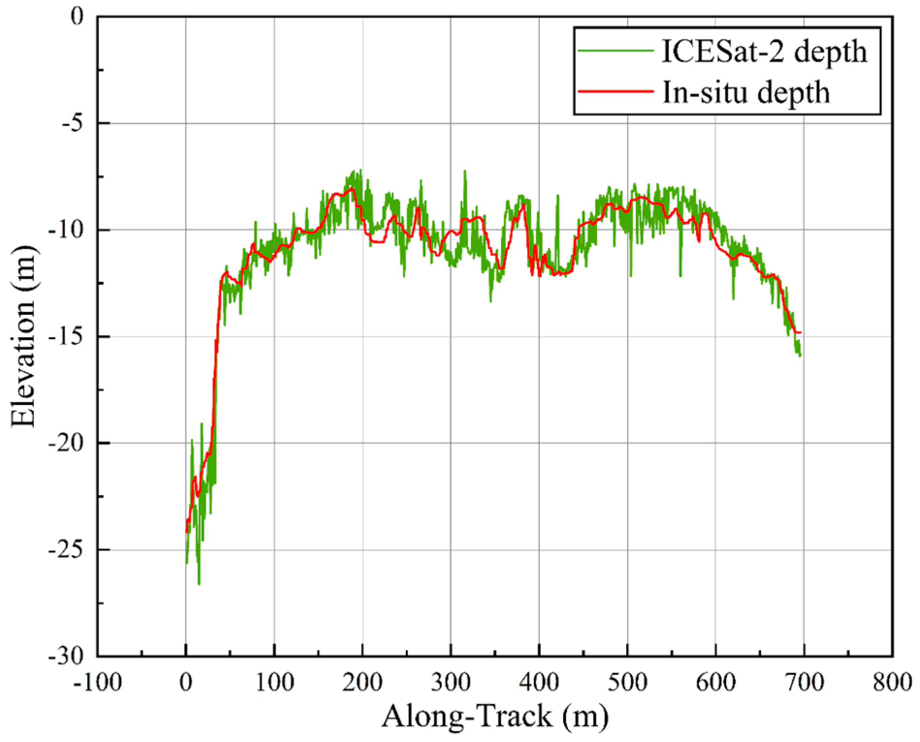
Figure 17 shows the data fitting results of the proposed method and the in situ bathymetry data. The experimental results indicate that the ICESat-2 sounding data after refractive index correction obtained by the proposed method align closely with the in situ sounding data, effectively displaying the underwater terrain contour information and providing a foundation for subsequent experiments.
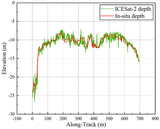
Figure 17.
Comparison between the ICESat-2 denoising results and in situ data.
4. Discussion
In this section, to further verify the photon denoising performance of the method proposed in this paper for different water depths, the accuracy of the reference visual interpretation data was quantitatively analyzed and discussed across different water depth ranges (<10 m, 10~20 m, and >20 m). The experimental results are shown in Figure 18. The experimental results show that the denoising effect of the proposed method surpasses that of other methods at different water depths. The denoising accuracy of the built-in ATL03 algorithm (confidence = 4) was found to be relatively low. The performances of the four denoising algorithms used in the experiment deteriorate with increasing water depth.
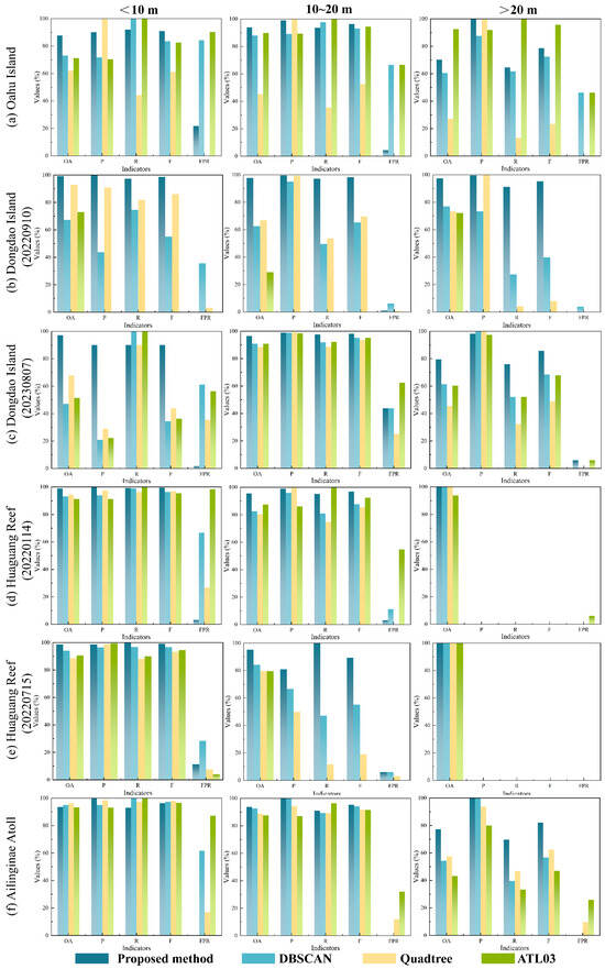
Figure 18.
Quantitative evaluation of the performances of the four methods at different water depths. (a) Represent the result of <10 m, 10–20 m, and >20 m in Oahu Island. (b) Represent the result of <10 m, 10–20 m, and >20 m on 10 September 2022 in Dongdao Island. (c) Represent the result of <10 m, 10–20 m, and >20 m on 7 August 2023 in Dongdao Island. (d) Represent the result of <10 m, 10–20 m, and >20 m on 14 January 2022 in Huaguang Reef. (e) Represent the result of <10 m, 10–20 m, and >20 m on 15 July 2022 in Huaguang Reef. (f) Represent the result of <10 m, 10–20 m, and >20 m in Ailinginae Atoll.
Figure 18a shows that the terrain of Oahu Island fluctuates widely. Within the 0~20 m range, the denoising performance of the proposed method surpasses that of the other three algorithms, while the quadtree algorithm’s performance remains relatively low. Above 20 m, the denoising performance of the proposed method declines slightly compared to that of the ATL03 built-in algorithm. This occurs because, in deep water areas, a small number of signal points are misclassified as noise. As shown in Figure 18b, the denoising performance of various algorithms on Dongdao Island indicates a significant advantage of the proposed method. The ATL03 algorithm solely identifies sea surface photons, resulting in precision indices approaching zero. As shown in Figure 18c, photons on Dongdao Island are concentrated in the 10~20 m range, and the denoising performance of various algorithms remains consistent. At depths less than 10 m and greater than 20 m, the proposed method exhibits superior denoising performance. As shown in Figure 18d, photons are concentrated within the 20 m range, where the performance of the proposed method slightly surpasses the other three algorithms. The FPR value of the ATL03 algorithm was found to be higher, indicating a higher probability of photon misidentification. As shown in Figure 18e, the photon point cloud of Huaguang Reef is concentrated within 10 m. Beyond the 10 m range, the proposed method shows a significant denoising effect. As shown in Figure 18f, the terrain of Ailinginae Atoll fluctuates widely. Within the 20 m range, the denoising performance of various algorithms remains consistent. Beyond the 20 m range, the proposed method exhibits good denoising performance, with higher OA, P, R, and F and lower FPR values than the other three algorithms.
5. Conclusions
This paper proposes a quadtree denoising algorithm based on the multiscale analysis of quadtree segmentation. Experiments indicate that this method effectively denoises the photon data obtained by ICESat-2 and removes underwater noise points while restoring underwater terrain information. The denoising results in this paper have a high correlation with the in situ bathymetry data, demonstrating that the signal photons extracted by this method can be directly used as water depth detection data in shallow coastal areas.
The quadtree algorithm segments the photon points in the two-dimensional plane space until the number of photons in the segmented subspace is within the maximum capacity. The density is represented by the corresponding layer values of photons in the subspace. Then, the maximum interclass variance is computed to separate the noise points from the signal points. However, due to the different photon densities in different experimental areas, direct quadtree segmentation may lead to misclassification of signal points, resulting in an excessive denoising effect. Therefore, considering the characteristics of the underwater photon density, which gradually decreases from shallow to deep, this paper proposes a quadtree segmentation algorithm based on multiscale analysis. First, the DBSCAN algorithm removes outlier noise points; then, the seafloor photons are divided into windows, and quadtree segmentation is performed within the window. The corresponding layer value of photons in the window is low, effectively reducing the probability of misclassification and enhancing the denoising accuracy.
Compared with the existing research results, the denoising method proposed in this paper addresses the problems of high dependence on parameters and vulnerability to noise distribution. Due to the complexity of the background photon distribution and the ability of ICESat-2 to detect signal photons, this method may still miss a small number of photons at the edge of underwater terrain within the detection range of ICESat-2. Subsequent research will focus on the extraction of such signals to improve the denoising effect of this method on photon data in more complex cases.
Author Contributions
Conceptualization, B.Z. and Y.L.; methodology, B.Z. and Z.D.; software, Z.D. and Y.L.; validation, B.Z., Y.L. and J.L.; formal analysis, Y.C. and Q.T.; investigation, B.Z. and Y.L.; resources, Y.C. and Q.T.; data curation, G.H. and J.T.; writing—original draft preparation, B.Z.; writing—review and editing, B.Z.; visualization, B.Z.; supervision, Y.L.; project administration, Y.L.; funding acquisition, Y.L., Z.D., J.L., Q.T. and Y.C. All authors have read and agreed to the published version of the manuscript.
Funding
This research was funded by the Open Fund of Shandong Provincial Key Laboratory of Marine Ecology and Environment and Disaster Prevention and Mitigation under Grant [No. 202304], the Foundation of Shandong Province under Grant [No. ZR2023QD113], the Shandong Postdoctoral Innovation Project under Grant [No. SDCX-ZG-202202041], the Natural Science Foundation of Qingdao Municipality under Grant [No. 23-2-1-73-zyyd-jch], and the National Key Research and Development Program of China under Grant [No. 2023YFC3107601].
Data Availability Statement
Data underlying the results presented in this paper are not publicly available at this time but may be obtained from the authors upon reasonable request.
Acknowledgments
We would like to express appreciation to the National Aeronautics and Space Administration (NASA) for providing the ICESat-2 data used in this article, as well as the in situ bathymetry data provided by the First Institute of Oceanography, Ministry of Natural Resources. Moreover, we thank the anonymous reviewers and members of the editorial team for their constructive comments.
Conflicts of Interest
The authors declare no conflicts of interest.
References
- Yang, Y.X.; Xu, T.H.; Xue, S.Q. Progresses and Prospects in Developing Marine Geodetic Datum and Marine Navigation of China. Acta Geod. Et Cartogr. Sin. 2017, 46, 1–8. [Google Scholar]
- Ma, Y.; Zhang, J.; Zhang, J.Y.; Zhang, Z.; Wang, J.J. Progress in shallow water depth mapping from optical remote sensing. Adv. Mar. Sci. 2018, 36, 331–351. [Google Scholar]
- Hodúl, M.; Bird, S.; Knudby, A.; Chénier, R. Satellite derived photogrammetric bathymetry. ISPRS J. Photogramm. Remote Sens. 2018, 142, 268–277. [Google Scholar] [CrossRef]
- Albright, A.; Glennie, C. Nearshore bathymetry from fusion of Sentinel-2 and ICESat-2 observations. IEEE Geosci. Remote Sens. Lett. 2020, 18, 900–904. [Google Scholar] [CrossRef]
- Caballero, I.; Stumpf, R.P. Retrieval of nearshore bathymetry from Sentinel-2A and 2B satellites in South Florida coastal waters. Estuar. Coast. Shelf Sci. 2019, 226, 106277. [Google Scholar] [CrossRef]
- Ranndal, H.; Sigaard Christiansen, P.; Kliving, P.; Baltazar Andersen, O.; Nielsen, K. Evaluation of a statistical approach for extracting shallow water ba-thymetry signals from ICESat-2 ATL03 photon data. Remote Sens. 2021, 13, 3548. [Google Scholar] [CrossRef]
- Parrish, C.E.; Magruder, L.A.; Neuenschwander, A.L.; Forfinski-Sarkozi, N.; Alonzo, M.; Jasinski, M. Validation of ICESat-2 ATLAS bathymetry and analysis of ATLAS’s bathymetric mapping performance. Remote Sens. 2019, 11, 1634. [Google Scholar] [CrossRef]
- Markus, T.; Neumann, T.; Martino, A.; Abdalati, W.; Brunt, K.; Csatho, B.; Farrell, S.; Fricker, H.; Gardner, A.; Harding, D.; et al. The Ice, Cloud, and land Elevation Satellite-2 (ICESat-2): Science requirements, concept, and implementation. Remote Sens. Environ. 2017, 190, 260–273. [Google Scholar] [CrossRef]
- Neumann, T.A.; Brenner, A.; Hancock, D.; Robbins, J.; Gibbons, A.; Lee, J.; Harbeck, K.; Saba, J.; Luthcke, S.B.; Rebold, T. ATLAS/ICESat-2 L2A Global Geolocated Photon Data, Version 6; NASA National Snow and Ice Data Center Distributed Active Archive Center: Boulder, CO, USA, 2023. [Google Scholar]
- Zhu, X.X.; Wang, C.; Xi, X.H.; Nie, S.; Yang, X.B.; Li, D. Research progress of ICESat-2/ATLAS data processing and applications. Infrared Laser Eng. 2020, 49, 76–85. [Google Scholar]
- Canny, J. A computational approach to edge detection. IEEE Trans. Pattern Anal. Mach. Intell. 1986, 8, 679–698. [Google Scholar] [CrossRef]
- Chen, B.; Pang, Y. A denoising approach for detection of canopy and ground from ICESat-2’s airborne simulator data in Maryland, USA. AOPC 2015 Adv. Laser Technol. Appl. SPIE 2015, 9671, 383–387. [Google Scholar]
- Magruder, L.A.; Wharton, M.E.; Stout, K.D.; Neuenschwander, A. Noise filtering techniques for photon-counting ladar data. Laser Radar Technol. Appl. XVII SPIE 2012, 8379, 237–245. [Google Scholar]
- Herzfeld, U.C.; McDonald, B.W.; Wallin, B.F.; Neumann, T.A.; Markus, T.; Brenner, A.; Field, C. Algorithm for detection of ground and canopy cover in micropulse pho-ton-counting lidar altimeter data in preparation for the ICESat-2 mission. IEEE Trans. Geosci. Remote Sens. 2013, 52, 2109–2125. [Google Scholar] [CrossRef]
- Gwenzi, D.; Lefsky, M.A.; Suchdeo, V.P.; Harding, D.J. Prospects of the ICESat-2 laser altimetry mission for savanna ecosystem structural studies based on airborne simulation data. ISPRS J. Photogramm. Remote Sens. 2016, 118, 68–82. [Google Scholar] [CrossRef]
- Xie, H.; Xu, Q.; Ye, D.; Jia, J.; Sun, Y.; Huang, P.; Li, M.; Liu, S.; Xie, F.; Hao, X.; et al. A comparison and review of surface detection methods using MBL, MABEL, and ICESat-2 pho-ton-counting laser altimetry data. IEEE J. Sel. Top. Appl. Earth Obs. Remote Sens. 2021, 14, 7604–7623. [Google Scholar] [CrossRef]
- Xie, H.; Ye, D.; Xu, Q.; Sun, Y.; Huang, P.; Tong, X.; Guo, Y.; Liu, X.; Liu, S. A density-based adaptive ground and canopy detecting method for ICESat-2 photon-counting data. IEEE Trans. Geosci. Remote Sens. 2022, 60, 4411813. [Google Scholar] [CrossRef]
- Ester, M.; Kriegel, H.P.; Sander, J.; Xu, X. A density-based algorithm for discovering clusters in large spatial databases with noise. In Proceedings of the KDD’96: Second International Conference on Knowledge Discovery and Data Mining, Portland, OR, USA, 2–4 August 1996; Volume 96, pp. 226–231. [Google Scholar]
- Ankerst, M.; Breunig, M.M.; Kriegel, H.P.; Sander, J. OPTICS: Ordering points to identify the clustering structure. ACM Sigmod Rec. 1999, 28, 49–60. [Google Scholar] [CrossRef]
- Zhang, J.; Kerekes, J.; Csatho, B.; Schenk, T.; Wheelwright, R. A clustering approach for detection of ground in micropulse photon-counting LiDAR altimeter data. In Proceedings of the 2014 IEEE Geoscience and Remote Sensing Symposium. IEEE, Quebec City, QC, Canada, 13–18 July 2014; pp. 177–180. [Google Scholar]
- Xie, F.; Yang, G.; Shu, R.; Li, M. An adaptive directional filter for photon counting Lidar point cloud data. J. Infrared Millim. Waves 2017, 36, 107–113. [Google Scholar]
- Chen, B.; Pang, Y.; Li, Z.; Lu, H.; Liu, L.; North, P.R.J.; Rosette, J.A.B. Ground and top of canopy extraction from photon-counting LiDAR data using local outlier factor with ellipse searching area. IEEE Geosci. Remote Sens. Lett. 2019, 16, 1447–1451. [Google Scholar] [CrossRef]
- Ma, Y.; Xu, N.; Sun, J.; Wang, X.H.; Yang, F.; Li, S. Estimating water levels and volumes of lakes dated back to the 1980s using Landsat imagery and photon-counting lidar datasets. Remote Sens. Environ. 2019, 232, 111287. [Google Scholar] [CrossRef]
- Zhu, X.; Nie, S.; Wang, C.; Xi, X.; Wang, J.; Li, D.; Zhou, H. A noise removal algorithm based on OPTICS for photon-counting LiDAR data. IEEE Geosci. Remote Sens. Lett. 2020, 18, 1471–1475. [Google Scholar] [CrossRef]
- Zhang, G.; Xu, Q.; Xing, S.; Li, P.; Zhang, X.; Wang, D.; Dai, M. A noise-removal algorithm without input parameters based on quadtree isolation for pho-ton-counting LiDAR. IEEE Geosci. Remote Sens. Lett. 2021, 19, 6501905. [Google Scholar]
- Huang, G.; Dong, Z.; Liu, Y.; Chen, Y.; Li, J.; Wang, Y.; Meng, W. An optimized denoising method for ICESat-2 photon-counting data considering heterogeneous density and weak connectivity. Opt. Express 2023, 31, 41496–41517. [Google Scholar] [CrossRef] [PubMed]
- Song, Y.; Ma, Y.; Zhou, Z.; Yang, J.; Li, S. Signal Photon Extraction and Classification for ICESat-2 Photon-Counting Lidar in Coastal Areas. Remote Sens. 2024, 16, 1127. [Google Scholar] [CrossRef]
- Xie, H.; Xu, Q.; Luan, K.; Sun, Y.; Liu, X.; Guo, Y.; Li, B.; Jin, Y.; Liu, S.; Tong, X. Evaluating ICESat-2 Seafloor Photons by Underwater Light-Beam Propagation and Noise Modeling. IEEE Trans. Geosci. Remote Sens. 2024, 62, 4203018. [Google Scholar] [CrossRef]
- Neumann, T.A.; Martino, A.J.; Markus, T.; Bae, S.; Bock, M.R.; Brenner, A.C.; Brunt, K.M.; Cavanaugh, J.; Fernandes, S.T.; Hancock, D.W.; et al. The Ice, Cloud, and Land Elevation Satellite–2 Mission: A global geolocated photon product derived from the advanced topographic laser altimeter system. Remote Sens. Environ. 2019, 233, 111325. [Google Scholar] [CrossRef] [PubMed]
- Chen, Y.; Le, Y.; Zhang, D.; Wang, Y.; Qiu, Z.; Wang, L. A photon-counting LiDAR bathymetric method based on adaptive variable ellipse filtering. Remote Sens. Environ. 2021, 256, 112326. [Google Scholar] [CrossRef]
- Hsu, H.J.; Huang, C.Y.; Jasinski, M.; Li, Y.; Gao, H.; Yamanokuchi, T.; Wang, C.-G.; Chang, T.-M.; Ren, H.; Kuo, C.-Y.; et al. A semi-empirical scheme for bathymetric mapping in shallow water by ICESat-2 and Sentinel-2: A case study in the South China Sea. ISPRS J. Photogramm. Remote Sens. 2021, 178, 1–19. [Google Scholar] [CrossRef]
- Leng, Z.; Zhang, J.; Ma, Y.; Zhang, J.; Zhu, H. A novel bathymetry signal photon extraction algorithm for photon-counting LiDAR based on adaptive elliptical neighborhood. Int. J. Appl. Earth Obs. Geoinf. 2022, 115, 103080. [Google Scholar] [CrossRef]
- Ma, Y.; Xu, N.; Liu, Z.; Yang, B.; Yang, F.; Wang, X.H.; Li, S. Satellite-derived bathymetry using the ICESat-2 lidar and Sentinel-2 imagery datasets. Remote Sens. Environ. 2020, 250, 112047. [Google Scholar] [CrossRef]
- Wang, B.; Ma, Y.; Zhang, J.; Zhang, H.; Zhu, H.; Leng, Z.; Zhang, X.; Cui, A. A noise removal algorithm based on adaptive elevation difference thresholding for ICESat-2 photon-counting data. Int. J. Appl. Earth Obs. Geoinf. 2023, 117, 103207. [Google Scholar] [CrossRef]
- Zhang, D.; Chen, Y.; Le, Y.; Dong, Y.; Dai, G.; Wang, L. Refraction and coordinate correction with the JONSWAP model for ICESat-2 bathymetry. ISPRS J. Photogramm. Remote Sens. 2022, 186, 285–300. [Google Scholar] [CrossRef]
- Zhang, X.; Chen, Y.; Le, Y.; Zhang, D.; Yan, Q.; Dong, Y.; Han, W.; Wang, L. Nearshore bathymetry based on ICESat-2 and multispectral images: Comparison between Sentinel-2, Landsat-8, and testing Gaofen-2. IEEE J. Sel. Top. Appl. Earth Obs. Remote Sens. 2022, 15, 2449–2462. [Google Scholar] [CrossRef]
- Zheng, X.; Hou, C.; Huang, M.; Ma, D.; Li, M. A density and distance-based method for ICESat-2 photon-counting data denoising. IEEE Geosci. Remote Sens. Lett. 2023, 20, 6500405. [Google Scholar] [CrossRef]
- Bargaoui, Z.K.; Chebbi, A. Comparison of two kriging interpolation methods applied to spatiotemporal rainfall. J. Hydrol. 2009, 365, 56–73. [Google Scholar] [CrossRef]
- Fang, Y.; Cao, B.; Gao, L.; Hu, H. Development and application of lidar mapping satellite. Infrared Laser Eng. 2020, 49, 19–27. [Google Scholar]
- Jiao, H.H.; Xie, J.F.; Liu, R.; Mo, F. Discussion on Denoising Method of Photon Counting LiDAR for Satellite Ground Observation. Spacecr. Recovery Remote Sens. 2021, 42, 140–150. [Google Scholar]
- Davis, R.A.; Lii, K.S.; Politis, D.N. Remarks on some nonparametric estimates of a density function. Selected Works of Murray Rosenblatt; Springer: New York, NY, USA, 2011; pp. 95–100. [Google Scholar]
- Parzen, E. On estimation of a probability density function and mode. Ann. Math. Stat. 1962, 33, 1065–1076. [Google Scholar] [CrossRef]
- Finkel, R.A.; Bentley, J.L. Quadtrees a data structure for retrieval on composite keys. Acta Inform. 1974, 4, 1–9. [Google Scholar] [CrossRef]
- Zhang, S.; Li, G.; Zhou, X.; Yao, J.; Guo, J.; Tang, X. Single photon point cloud denoising algorithm based on multi-features adaptive. Infrared Laser Eng. 2022, 51, 20210949. [Google Scholar]
- Zhu, X.; Nie, S.; Wang, C.; Xi, X.; Hu, Z. A ground elevation and vegetation height retrieval algorithm using micro-pulse photon-counting lidar data. Remote Sens. 2018, 10, 1962. [Google Scholar] [CrossRef]
- Otsu, N. A threshold selection method from gray-level histograms. Automatica 1975, 11, 23–27. [Google Scholar] [CrossRef]


Disclaimer/Publisher’s Note: The statements, opinions and data contained in all publications are solely those of the individual author(s) and contributor(s) and not of MDPI and/or the editor(s). MDPI and/or the editor(s) disclaim responsibility for any injury to people or property resulting from any ideas, methods, instructions or products referred to in the content. |
© 2024 by the authors. Licensee MDPI, Basel, Switzerland. This article is an open access article distributed under the terms and conditions of the Creative Commons Attribution (CC BY) license (https://creativecommons.org/licenses/by/4.0/).