Prediction of Deformation in Expansive Soil Landslides Utilizing AMPSO-SVR

Abstract

A non-periodic “step-like” variation in displacement is exhibited owing to the repeated instability of expansive soil landslides. The dynamic prediction of deformation for expansive soil landslides has become a challenge in actual engineering for disaster prevention and mitigation. Therefore, a support vector regression prediction (AMPSO-SVR) model based on adaptive mutation particle swarm optimization is proposed, which is suitable for small samples of data. The shallow displacement is decomposed into a trend component and fluctuating component by complete ensemble empirical mode decomposition with adaptive noise (CEEMDAN), and the trend displacement is predicted by cubic polynomial fitting. In this paper, the multiple disaster-inducing factors of expansive landslides and the time hysteresis effect between displacement and its influencing factors are fully considered, and the crucial influencing factors which eliminate the time lag effect and state factors are input into the model to predict the fluctuation displacement. Monitoring data in the Ningming area of China are employed for the model validation. The predicted results are compared with those of the traditional model. The model performance is evaluated through indicators such as the goodness of fit R² and root mean square error RMSE. The results show that the prediction RMSE of the new model for three monitoring stations can reach 2.6 mm, 6.6 mm, and 2.5 mm, respectively. Compared with the common Grid search support vector regression (GS-SVR), the Particle Swarm Optimization Support Vector Regression (PSO-SVR) and Back Propagation Neural Network (BPNN) models have average improvements of 58.4%, 38.1%, and 25.2% respectively. The goodness of fit R² is superior to 0.99 in the new method. The proposed model can effectively be deployed for the displacement prediction of non-periodic stepped expansive soil landslides driven by multiple influencing factors, providing a reference idea for the deformation prediction of expansive soil landslides.

1. Introduction

Expansive soil landslides are a complex clay geological hazard distributed in more than 20 provinces in China, where nearly 400 million people live. Uneven settlements of buildings, instability of engineering slopes, and other detriments are easily attributed to the unstable deformation characteristics of expansive soil due to water absorption expansion deformation and water loss shrinkage cracking [1].

To effectively prevent expansive soil landslide hazards, it is crucial to accurately predict future displacements by utilizing historical landslide data. Expansive soil landslides are unstable nonlinear systems with complex instability mechanisms and special engineering characteristics of repeated expansion and contraction; these special “step-like” characteristics are presented in displacement curves [2]. Compared with traditional loess landslides, the step-like rise in the displacement of expansive soil landslides does not follow strict rainfall periodicity and is often accompanied by strong burstiness [3,4,5,6,7,8]. This is because expansive soil landslides are jointly affected by multiple internal and external factors. In addition to precipitation, landslide stability is also significantly impacted by earth pressure and soil moisture content [9,10,11,12]. Therefore, the dynamic prediction of the displacement of step-like expansive soil landslides driven by multiple factors is an important technical issue that needs to be solved urgently in the current research on landslide prediction.

Solutions for the prediction of step-like landslide displacement have been researched by numerous scholars so far. For example, Zhu Xing proposed an extreme learning machine (ELM) to predict the displacement of the Baijiabao landslide in the Three Gorges [13], Gao Wei fused a grey system (GM) with an evolutionary neural network (ENN) to predict two landslides in the Three Gorges Reservoir Area [14], and Yang Beibei constructed a long short-term memory network (LSTM) for the displacement prediction of the Baishui river landslide [15]. Nevertheless, single factors such as the reservoir water level and rainfall were mainly considered in the above methods, but they are more suitable for landslides with more obvious deformation cycles and a single influencing factor. The internal characteristics of landslides, such as non-periodic soil stress or the internal moisture field of slopes, have not been fully considered. The above neural-network-based prediction models have complex algorithm structures and require high-quality feature data and sample sizes, which is not suitable for predicting the displacement of non-periodic expansive soil landslides under the joint influence of multiple internal and external factors. A strong generalization ability is exhibited by Support Vector Regression (SVR) [16], and the nonlinear relationship between multiple external factors and target displacement can be handled effectively. It does not require complex operation for preprocessing and feature selection in an input dataset, and the model has an excellent robustness. It is very suitable for predicting the deformation of step-like landslides dominated by multiple factors. However, it is easy for the traditional SVR model to fall into local optimal, which can be solved effectively by adaptive mutation particle swarm optimization (AMPSO) [17,18].

Therefore, a machine learning prediction algorithm based on AMPSO-SVR is proposed to predict the displacement of expansive soil landslides. The main idea includes: (1) The total displacement being decomposed into trend and fluctuation terms, respectively, by complete ensemble empirical mode decomposition with adaptive noise (CEEMDAN). (2) The trend displacement being predicted by a fitting method and the relationship between the fluctuation term and the influencing factors being analyzed. (3) The time delay effect between the displacement and multi-factor being considered, the multi-factor wave term component being extracted by CEEMDAN and input into the AMPSO-SVR model to predict the wave term displacement, and the prediction results being compared with grid search support vector regression (GS-SVR), and particle swarm optimization support vector regression (PSO-SVR), verifying that the “step-like” non-periodic displacement can be accurately and dynamically predicted, which has a certain feasibility and scientificity. (4) The total predicted displacement sequence being obtained by superimposing the predicted values of the trend and fluctuation terms.

2. Displacement Prediction Model of Expansive Soil Landslides

2.1. Displacement Time Series Theory

The displacement of expansive soil exhibits nonlinear characteristics under the influence of crack evolution and wet–dry cycles. The total displacement is decomposed into a trend term, wave term displacement, and random term displacement according to the time series theory [19,20].

$$S\left(t\right)=T\left(t\right)+P\left(t\right)+R\left(t\right)$$

(1)

where S(t) is the total displacement value, T(t) is the trend term displacement, and P(t) is the fluctuation term displacement. The magnitude of R(t) is small and negligible, and the prediction of T(t) and P(t) is mainly focused on in this paper.

2.2. Complete Ensemble Empirical Mode Decomposition with Adaptive Noise

Moving average, wavelet decomposition, and EMD are commonly applied to landslide displacement decomposition [21]. EMD decomposition is a conventional method for decomposing non-stationary data. However, anomalies in displacement decomposition may be caused by the existence of mode aliasing, and the displacement trend term and the fluctuation term can be extracted inaccurately. Moving average has a poor adaptability to noise, and wavelet decomposition has challenges in processing non-stationary signals such as landslide displacement curves. The above problems can be effectively overcome by CEEMDAN decomposition. Adaptive noise is added to landslide displacement curves, which improves the robustness of decomposition and is more suitable for processing non-stationary signals. These decomposed displacement components are more consistent with the actual change trends of landslides. The CEEMDAN decomposition flow is designed as follows in this paper:

(1) The landslide displacement S(t) is added with Gaussian white noise, whose K-th mean is 0 to construct the K sequence S_i(t) to be decomposed. i = 1, 2, 3, … k, ε is the signal-to-noise ratio, and δ_i(t) is the white noise sequence added for the i-th time.

$$S_i\left(t\right)=S\left(t\right)+\epsilon {\delta }_i\left(t\right)$$

(2)

(2) The EMD decomposition of S_i(t) is performed, the first modal component (IMF) is decomposed, and its mean is taken as the first modal component obtained by CEEMDAN decomposition. Each modal component is a different frequency component of the original displacement. r₁(t) is the first residual component, which represents the non-extractable aperiodic component of the displacement sequence.

$$IM{F}_1\left(t\right)=\frac{1}{K}{\displaystyle \sum }_{i=1}^{K}IM{F}_1^i\left(t\right)$$

(3)

$$r_1\left(t\right)=S\left(t\right)-IM{F}_1\left(t\right)$$

(4)

(3) The EMD decomposition is continued after noise is added to the residual component r_j(t) of phase j.

$$IM{F}_j\left(t\right)=\frac{1}{k}{\displaystyle \sum }_{i=1}^K{E}_1\left(r_{j-1}\left(t\right)+{\epsilon }_{j-1}{E}_{j-1}\left({\delta }_i\left(t\right)\right)\right)$$

(5)

$$r_j\left(t\right)=r_{j-1}\left(t\right)-IM{F}_j\left(t\right)$$

(6)

(4) If the EMD stop condition is satisfied and the displacement residual component r_n(t) of the n-th decomposition is close to a monotone signal, then the CEEMDAN algorithm ends its decomposition.

2.3. Support Vector Regression (SVR)

Expansive soil landslides are driven by various correlation factors [22]. The relationship between displacement and external factors is not a simple linear form, but a more complex curve shape, such as a polynomial or periodic relationship, etc., which can be solved effectively by Support Vector Regression (SVR). SVR began with the research of Drucker et al. (1997) [23]. The principle is to find a nonlinear mapping from the input space to the output space, and the feature data x are mapped to a high-dimensional feature space, and the regression plane with the optimal fitting performance in the high-dimensional space is selected. Its mathematical model is as follows:

$$P\_pre\left(x\right)={\omega }^T\phi \left(x\right)+b$$

(7)

where $P\_pre\left(x\right)$ is the output value of the model, namely, the predicted displacement value of the landslide fluctuation term corresponding to the predicted value of item P(t) in Equation (1), ω is the inertia weight, b is the offset term, and φ(x) is the mapping function between the landslide correlation factor x and predicted displacement, which includes the input values of the model, namely, the data of multiple influence factors that affect expansive soil landslides and the historical displacement data. The data of multiple influence factors are mapped to a high-dimensional feature space for linear analysis in that space. The nonlinear relationship between displacement and multi-factor features can be modeled accurately by utilizing the kernel function in the SVR model. The key to SVR machine learning is to find the optimal nonlinear mapping relationship so that the output displacement f(x) is closer to the actual value.

2.4. Adaptive Mutation Particle Swarm Optimization (AMPSO)

The particle swarm optimization algorithm (PSO) is an evolutionary algorithm inspired by bird foraging [24]. The solution is regarded as a particle, the particle quality is measured by the particle fitness, and the optimal solution is obtained through multiple iterations. However, the particles are likely to quickly gather near a local optimum in the early stages of the search process, and the search space is not fully explored. It is easy to fall into the local optimum, which makes it difficult to obtain the global optimal solution. The adaptive mutation particle swarm optimization (AMPSO) is an improvement of the standard PSO, and it adjusts the search range of the solution space by dynamically adjusting the weight and adaptive mutation mechanism so that the algorithm has a large global search ability, which can address this issue. The strategy adopted by the algorithm is to adjust the inertia weight adaptively. The larger weight is beneficial for improving the global optimization ability of the particle that can make it skip the local optimum. Therefore, a better optimal position on a large scale can be explored by taking a larger value of ω initially, while a smaller weight will improve the local optimal ability of particles so that the search process can be gradually converged. Later, the value of ω will decrease to improve the convergence accuracy. The weight linear attenuation method is adopted in this paper according to the iterative process, and its mathematical model is as follows:

$$\begin{array}{c}{V}_{id}^{k+1}=\omega V_{id}^k+c_1{r}_1\left(P_{id}^k-W_{id}^k\right)+c_2{r}_2\left(P_{gd}^k-W_{gd}^k\right)\\ W_{id}^{k+1}=W_{id}^k+V_{id}^{k+1}\end{array}$$

(8)

$${\omega }_{iner}={\omega }_{start}-\frac{\left({\omega }_{start}-{\omega }_{end}\right)·I}{N}$$

(9)

where i is the number of particles, d is the dimension of the prediction space, k is the number of iterations, v is the particle velocity, W is the particle position, ω is the inertia weight, Equation (9) is the updating method for weight ω in Equation (8), ω_iner is the inertial weight of adaptive change, ω_start is the maximum weight (value is 0.9), and ω_end is the minimum weight value (value is 0.4). The inertia weight in Equation (8) can be linearly decreased in this way, and the tradeoff between global search and local search can be balanced in the iterative process. This strategy of decreasing weights is aimed at giving the algorithm a greater exploration ability in the initial stage, and gradually increasing the focus on local search in subsequent iterations. Oscillation near the global optimal solution in the late particle search is effectively avoided. I is the current number of iterations, N is the total number of iterations, c₁ is the learning factor 1, and c₂ is the learning factor 2. r₁ and r₂ are random floating point numbers ranging from 0 to 1, P is the optimal position of the particle individual, and g is the global optimal position of the particle swarm.

Simultaneously, random particle mutation should be added to the particle position and velocity search in the iterative process to increase the diversity of the population. The mutation method selected is as follows:

$$if R<C_m, \left\{\begin{array}{c}ceil\left(2\times R\right)=1,v_c=R\times \left(C_{max}-C_{min}\right)+C_{min}\\ ceil\left(2\times R\right)=2,v_g=R\times \left(g_{max}-g_{min}\right)+g_{min}\end{array}\right.$$

(10)

In the formula, R is the random number of distributions [0, 1], C_m is the preset mutation probability (constant, set as 0.8 in this paper), $v_c$ is the particle motion velocity of hyperparameter c, $v_g$ is the velocity of the particle with the hyperparameter gamma, and C_min, C_max, g_min, and g_max are the search boundaries of the parameters. The adaptive mutation search for the optimal particles is implemented by this method, which enables the SVR model to jump out of the local optimum and find the best parameters c and g. These parameters enable the model to find the best mapping function φ(x). The risk of easily falling into overfitting is reduced. The adaptive mutation particle swarm optimization utilizes adaptive optimization to enable the SVR to select parameters more robustly, reducing the problem of model performance degradation caused by improper parameter selection. This is particularly significant for small sample data, as they are more sensitive to parameter selection. The prediction accuracy is further improved.

2.5. The Flow of Prediction Method

The process of the proposed prediction model is shown in Figure 1. The steps are as follows: (1) GNSS (Global Navigation Satellite System) displacement and earth pressure, precipitation, soil moisture content, and other data are collected by multi-source sensors. Among them, the displacement is obtained by self-developed GNSS monitoring equipment with a Ublox ZED-F9P board, and the measurement accuracy is better than 5 mm in both the horizontal and vertical directions. The soil moisture content is obtained by soil moisture meters, with a measurement accuracy of ±3%. The earth pressure is measured by earth pressure boxes, with a nominal measurement accuracy of ±0.5% F.S. The precipitation is obtained by funnel-type rain gauges, with an accuracy of measurement of ±0.2 mm. The multi-source data are processed on a self-built expansive soil landslide monitoring cloud platform; the GNSS displacement is calculated by real-time relative positioning with a solution frequency of 1 s and the GNSS receiver is mainly deployed at the leading edge and the middle of the slope, where the stability of expansive soil landslides is poor. A soil hygrometer determines the soil moisture content by measuring the change in the soil dielectric constant; its measurement frequency is 4 h and it should be deployed 30 cm below the surface of the expansive soil. The earth pressure box converts the mechanical pressure into an electrical signal and converts the electrical signal into the actual pressure value through calibration, with a measurement frequency of 4 h. The box is laid in the middle of the soilbag and reinforced with steel bars. The rain gauge collects precipitation through a tipping bucket structure. Its measurement frequency is 6 h and it is deployed in a stable and open location. (2) The landslide displacement is decomposed into a trend term and wave term, respectively, with CEEMDAN. The trend term displacement represents the long-term trend of landslide development and is predicted by the polynomial fitting method. (3) The correlation and the influence lag time between the fluctuation displacement and external factors are determined. The wave term component of multiple factors is the key part that affects changes in the fluctuation term displacement, which is similarly extracted by CEEMDAN and will be set as the optimal correlation factor to predict the step-like displacement of expansive soil landslides. (4) The AMPSO-SVR model is established by considering the state factors of landslide development. (5) Finally, the performance of the prediction model is evaluated with indicators like R², MAPE, and RMSE.

2.6. Evaluation Indicators for Displacement Prediction

Three evaluation indicators were used to evaluate the prediction accuracy of the proposed model R² (goodness of fit), RMSE (root mean square error), and MAPE (mean absolute percentage error). Their mathematical expressions are shown in Equations (11)–(13):

$$R^2=1-\frac{{{\displaystyle \sum }}_{i=1}^n{\left(y_i-{\widehat{y}}_i\right)}^2}{{{\displaystyle \sum }}_{i=1}^n{\left(y_i-\overline{y}\right)}^2}$$

(11)

$$RMSE=\sqrt{\frac{1}{n}{\displaystyle \sum }_{i=1}^n{\left(y_i-{\widehat{y}}_i\right)}^2}$$

(12)

$$MAPE=\frac{1}{n}{\displaystyle \sum }_{i=1}^n\left|\frac{{\widehat{y}}_i-y_i}{y_i}\right|$$

(13)

where y_i is the measured displacement, ${\widehat{y}}_i$ is the predicted displacement, $\overline{y}$ is the average displacement, which corresponds to the fluctuation term displacement, and i is the monitoring period.

3. Experimental Analysis—Expansive Soil Landslide on Chongai Highway in Ningming

3.1. Landslide Overview

The Ningming expansive soil landslide is located in Ningming Basin, Guangxi Province, China, which has the largest expansive soil deposit in the world and is a typical expansive soil research area. The expansive soil in this area belongs to the type of residual expansive soil [25]. It is a medium expansive soil with a free expansion coefficient of about 58%. The geographical location and overview of the slope are shown in Figure 2. The specific location of the landslide is about 5.2 km on the north bank of the Mingjiang River, a tributary of the Pearl River, 1 km west of Wayao Village, and near the Chongzuo–Aidian highway. Mainly in the shape of a long and narrow fan, it is a highway cutting landslide with a slope of about 1:1.5.

The region has a tropical marine monsoon climate with an average annual precipitation of 1200 mm and with spring and summer from April to October and autumn and winter from November to March. A total of eight GNSS monitoring points (NN01–NN08) were deployed to establish a real-time displacement-monitoring system with a monitoring accuracy better than 5 mm due to the obvious displacement of slope unloading. In addition, sensors such as those for earth pressure and soil moisture content were installed to strengthen the monitoring system, and the data transmission interval was 4 h. A rain gauge was arranged at the rear edge, and the data transmission interval was 1 h.

3.2. Deformation Characteristics

The GNSS cumulative displacement curve of the Ningming expansive soil slope is shown in Figure 3, which was calculated by the real-time GNSS landslide cloud platform. Due to the low stability at the three monitoring points on the top position of the slope, there was a significant increase in displacement compared to other points, hence, these three points were selected as the experimental dataset. The red, green, and blue curves represent the displacements of the NN06, NN07, and NN08 monitoring points, showing a step-like characteristic. They are located in sections ➃–➄ of the slope, where the risk of instability is high as a result of excavation unloading, and the slide direction is 78° north by west. The interstitial rise in displacement was mainly due to the occurrence of heavy rainfall events around 25 d and 155 d in the figure. The fissure of expansive soil provided an excellent channel for rainwater infiltration, resulting in a rapid increase in soil water content and a decrease in matrix suction as a result of the decrease in slope shear strength with an increase in saturation. The whole process time was relatively short, so the cumulative displacement increased rapidly with a strong mutability. There was no significant change in displacement during the drying period.

The on-site failure form of the slope is shown in Figure 4. The soil near the GNSS monitoring equipment was significantly cracked, and fish-scale shallow failure characteristics appeared after two instability events. Many cracks developed obviously, and these cracks gradually closed and deepened with an increase in instability frequency, finally collapsing in the form of a traction landslide.

4. Displacement Prediction

A multi-factor support vector regression prediction model was established with the GNSS cumulative displacement, soil moisture content, earth pressure, precipitation, and other data of monitoring points NN06–NN08 for about 200 days. The first 150 days of data were selected as the training set, the last 50 days were selected as the prediction set. The 75% training set ratio helped the model to better learn the pattern of the data, leaving a smaller proportion (25%) of sufficient samples to evaluate the generalization ability of the model, with the problem of overfitting of the training set being effectively avoided. Furthermore, the displacement of expansive soil experienced irregular changes such as a smooth and steep rise in the first 150 days, including the dynamic changes of expansive soil landslides from the safety stage to the instability stage. Hence, the selection of training and prediction sets in this way was more representative.

4.1. Extraction and Prediction of Trend Displacement

The trend term and fluctuation term of the displacement time series were extracted by CEEMDAN decomposition. The decomposition results are shown in Figure 5, from which it can be seen that the trend displacement component was nearly monotonically increasing, while the fluctuation term displacement was characterized by intermittent oscillation.

The trend displacement was fitted by the least squares cubic polynomial according to the nonlinear curve characteristics of the trend displacement at the monitoring points NN06, NN07, and NN08. The fitting expression is s(t) = at³ + bt² + ct + d, where s(t) is the trend term displacement, t is the monitoring time, and a, b, c, and d are the coefficients. The prediction results and accuracy of the trend term displacement are shown in Figure 6. The fitting accuracy RMSEs of the NN06, NN07, and NN08 monitoring points were 0.68 mm, 0.51 mm, and 0.46 mm, respectively, and the goodness of fit R² were 0.9989, 0.9959, and 0.9976, respectively.

4.2. Extraction and Prediction of Fluctuation Term Displacement

The fluctuation term displacement was obtained by subtracting the trend term displacement from the total displacement, which reflects the landslide displacement changes under the influence of external factors. In this paper, a multi-factor machine learning dynamic prediction model was established for the GNSS fluctuation term displacement at NN06, NN07, and NN08 for 200 d. The displacement data of the first 150 d were selected as the training set, and the last 50 d were selected as the test set.

4.2.1. Determination of Key Disaster-Inducing Factors

The prediction performance of the landslide displacement of expansive soil is directly affected by the selection of disaster-inducing factors [26]. Strength attenuation and swelling deformation are caused by unsaturated seepage under rainfall conditions, which has a significant impact on landslide stability. Moreover, the infiltration effect of rainwater is enhanced by the existence of cracks in expansive soil, and the effective water content of the soil is increased, which leads to the hygroscopic expansion of soil. The volume deformation of expansive soil under the dry–wet cycle has a significant impact on the pressure distribution of the retaining wall, and the lateral earth pressure increases significantly under the action of infiltrating rainwater and the mass of the overlying soil [27,28,29]. Therefore, precipitation, soil moisture content, and earth pressure are regarded as key factors for displacement prediction.

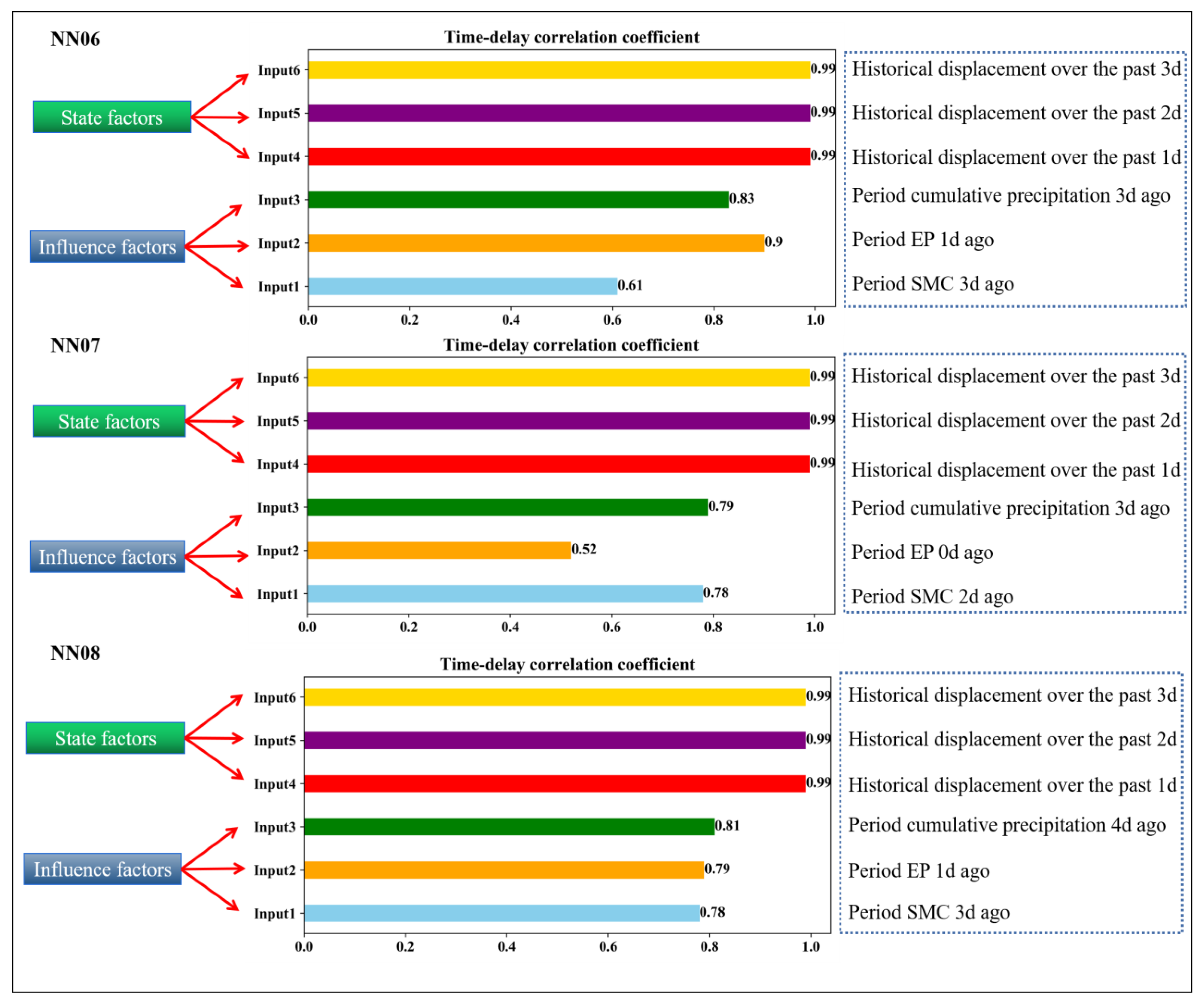
4.2.2. Time Lag Correlation

During the deformation process of an expansive soil landslide induced by rainfall, the soil moisture content and earth pressure first begin to increase, there is a lag time in the corresponding displacement changes, and the lag time is different at several monitoring points. To find the best correlation factor of the landslide displacement for the model training and avoid obvious deviations in the prediction results, the displacement response lag times of each monitoring point were determined by time delay correlation analysis (TDCA). The results are shown in Figure 7 (Unit: d): for the NN06, NN07, and NN08 monitoring points, the time lag parameters of the fluctuation term displacement and soil moisture content, earth pressure, and cumulative rainfall were (3 d, 1 d, 3 d), (2 d, 0 d, 3 d), and (3 d, 1 d, 4 d), respectively.

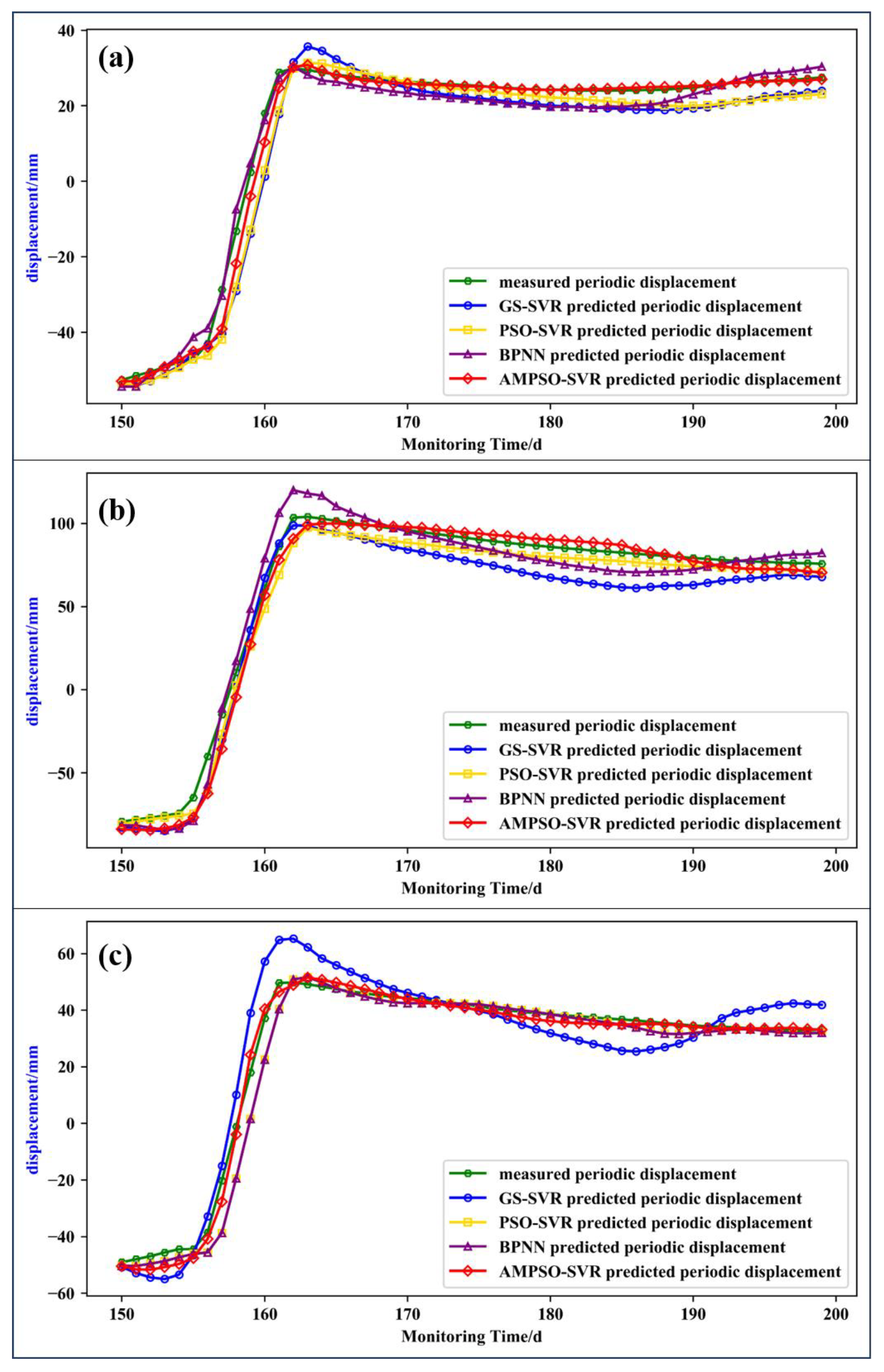
4.2.3. Fluctuation Term Displacement Prediction

Compared with the neural network prediction model, the prediction problem of multi-dimensional features can be solved by SVR more efficiently, and the prediction model is built by combining the AMPSO optimization algorithm. Since each non-periodic step change of the expansive soil slope displacement is greatly impacted by the fluctuation term of the external multi-source factor, the fluctuation term of the influencing factor is extracted by CEEMDAN. The mutation information of the influencing factors can be reflected by the fluctuation term component of the multi-factor, which is strongly related to the mutation of the fluctuation term displacement. Hence, it is more suitable for predicting the wave term displacement. As shown in Figure 8, the blue, green, orange, and red circled curves represent the fluctuation term displacement, fluctuation term cumulative precipitation, fluctuation term soil moisture content, and fluctuation term earth pressure at the monitoring points. The correlation between the wave term displacement and the influence factors sequence was more notable when the time lag was eliminated. It can be seen that the fluctuation term cumulative precipitation, soil moisture content, and fluctuation term periodic earth pressure started to increase, and the fluctuation term displacement showed a sudden increase simultaneously. If the cumulative precipitation, soil moisture content, and earth pressure of the fluctuation items continued to decrease overall, although there was a small local rebound, the corresponding fluctuation term displacement decreased synchronously and rose synchronously again during the next instability. Therefore, the fluctuation term displacement was more consistent with the fluctuation term change trend of external influence factors.

A self-learning AMPSO-SVR displacement prediction model was established based on the libsvm toolkit in matlab2021b software by normalizing the multi-factor association data and displacement data which eliminated the time lag effect. The model in this section was trained on a Hewlett-Packard computer with an Intel core i7-11800H processor (clocked at 2.3 GHz, eight cores, and sixteen threads), an NVIDIA RTX3050 GPU, and 16 G of memory. The fitness function is defined as the mean square error between the predicted and measured displacement values.

Taking into account the different lag times of the displacements for each monitoring point, multi-factor data that eliminated the time lag effect were added to the training model. The multi-factor data to eliminate the delay effect were added to the training model while considering the different lag times of the displacements at each monitoring point. For the NN06 monitoring point, six types of data, including the fluctuation item soil moisture content (SMC), fluctuation item cumulative precipitation 3 days ago, fluctuation item earth pressure (EP) 1 day ago, and historical displacements in the past 1 d, 2 d, and 3 d, were taken as model inputs. Similarly, for the NN07 monitoring point, the fluctuation term soil moisture content 2 days ago, fluctuation term cumulative precipitation 3 days ago, and fluctuation term earth pressure 1 day ago were combined. For the NN08 point, the fluctuation term soil moisture content 3 days ago, cumulative precipitation of the fluctuation term 4 days ago, and earth pressure data of the fluctuation term 2 days ago were input into the model for data training.

However, it is not reliable to predict the displacement by only considering the influencing factors and ignoring the development state of the landslide itself. The historical displacements before 3 d, 2 d, and 1 d were added into the model as predicted state factors. A total of six sequences were taken as inputs to the AMPSO-SVR model (Figure 9). After 150 iterations of parameter optimization, the final displacement prediction value was obtained.

To evaluate the actual performance of the prediction model, the results were compared with the commonly used GS-SVR, PSO-SVR, and BPNN models (see Figure 10). The goodness of fit R², root mean square error RMSE, and mean absolute percentage error MAPE were calculated. The calculation formula is as shown in Equation (10). The calculation results of related indicators are shown in

Table 1. Evaluation indicators of different prediction models.

Monitoring Points	R2	RMSE (mm)	MAPE	Model
NN06	0.9524	5.9	0.3131	GS-SVR
	0.9626	5.2	0.2661	PSO-SVR
	0.9864	3.1	0.1273	BPNN
	0.9907	2.6	0.1017	AMPSO-SVR
NN07	0.9459	13.2	0.1793	GS-SVR
	0.9821	7.6	0.1124	PSO-SVR
	0.9776	8.9	0.1254	BPNN
	0.9857	6.6	0.1181	AMPSO-SVR
NN08	0.9239	8.5	0.3766	GS-SVR
	0.9697	5.3	0.3871	PSO-SVR
	0.9872	3.8	0.2135	BPNN
	0.9934	2.5	0.0964	AMPSO-SVR

. As can be seen from the prediction results in Figure 10, the green circle curve is the measured displacement data of the landslide, the blue circle curve is the prediction result of the GS-SVR model, the yellow square curve is the prediction result of the PSO-SVR model, the purple triangle curve is the prediction result of the BPNN model, and the red diamond curve is the prediction result of the AMPSO-SVR model. Among them, the predicted results of the GS-SVR model at the monitoring points NN06 and NN08 during the instability period were significantly greater than the measured displacement, and the predicted displacement was not stable in the short time after the slope failure, which is not consistent with the characteristics of the displacement tending to be stable after the actual landslide failure. The goodness of fit and root mean square error at point NN06 were 0.9524 and 5.9 mm, respectively. The goodness of fit and root mean square error at point NN07 were 0.9459 and 13.2 mm, respectively. The goodness of fit and root mean square error at point NN08 were 0.9239 and 8.5 mm, respectively. The prediction error was larger among the four prediction models.

The predicted results of PSO-SVR were similar to the measured results, but the goodness of fit and root mean square error were inferior to the results of the AMPSO-SVR model. The BPNN prediction results showed a good performance at points NN06 and NN08, but a poor performance at point NN07. It can be seen that the predicted value at point NN07 was significantly higher than the measured value during the sliding stage, which had significant errors. Therefore, the generalization ability of this model was insufficient.

The AMPSO-SVR prediction results were most consistent with the measured displacements at the three monitoring points. The goodness of fit and root mean square error at point NN06 were 0.9907 and 2.6 mm, respectively. The goodness of fit and root mean square error at point NN07 were 0.9857 and 6.6 mm, respectively. The goodness of fit and root mean square error at point NN08 were 0.9934 and 2.5 mm, respectively. With the maximum goodness of fit and minimum root mean square error, the comprehensive generalization ability of the model was better than that of the other three models. Hence, the prediction performance of the AMPSO-SVR model was superior to other models.

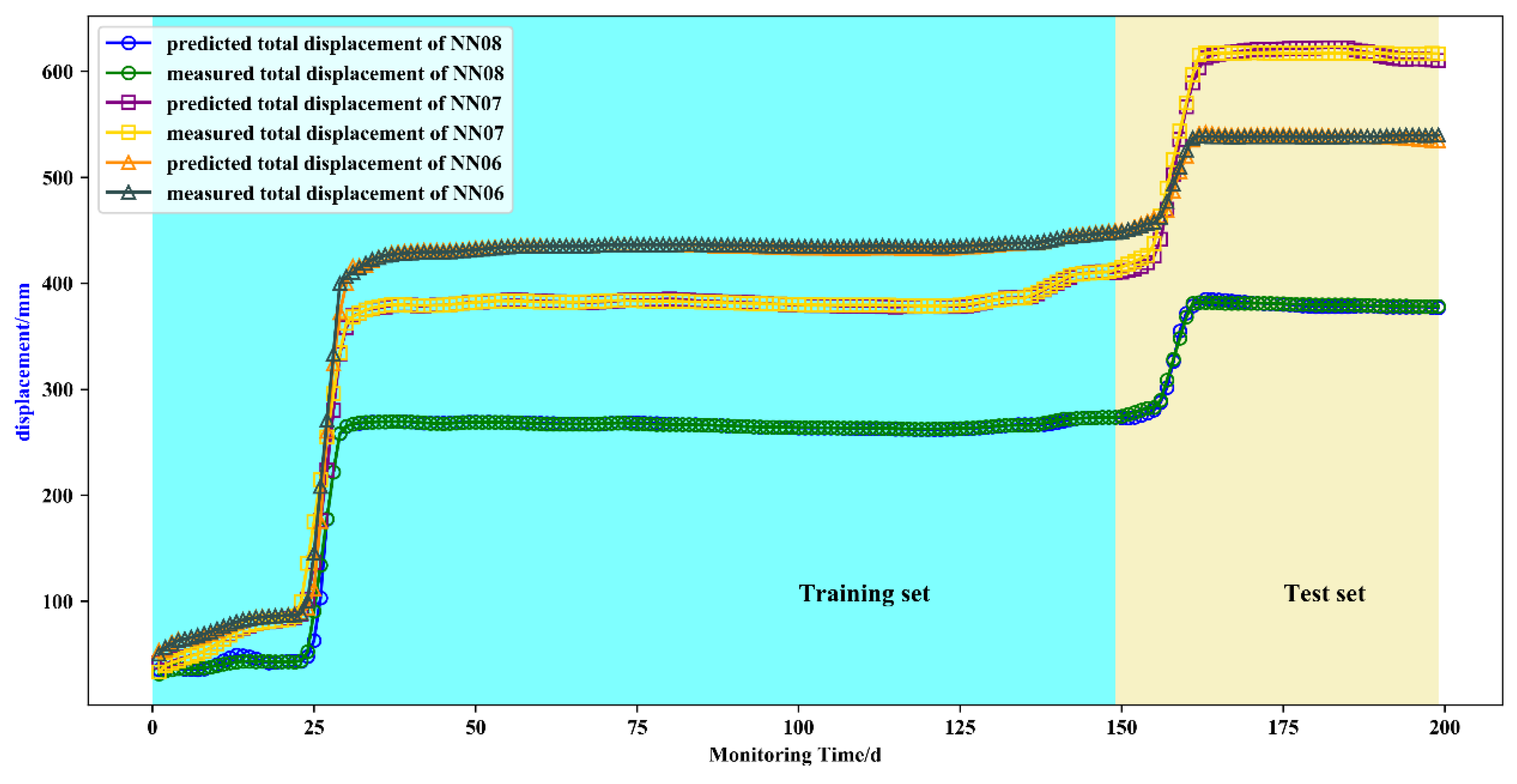
4.3. Total Displacement Prediction and Accuracy Analysis

The predicted value of the total displacement was obtained by superpositioning the predicted value of the displacement of the fluctuation term and the trend term, which was compared with the measurements. The prediction result curves are shown in Figure 11. The goodness of fit R² and RMSE of the predicted and measured displacements of the NN06, NN07, and NN08 monitoring points were 0.99, 2.6 mm, 0.99, 6.6 mm, and 0.99, 2.5 mm, respectively. These prediction results were consistent with the actual measurements, and the accuracy was in the order of millimeters. This indicated that the AMPSO-SVR prediction model can be well applied to multi-factor-driven non-periodic step-like expansive soil landslide displacement prediction.

5. Conclusions

(1)

The characteristics of the “ladder-type” deformation of expansive soil landslides due to their non-periodic repeated instability were recorded and analyzed. The important relationship between key influencing factors such as earth pressure, soil moisture content, and cumulative precipitation with this step displacement were also revealed. Meanwhile, the lag response time of landslide displacement and influencing factors was determined. The GNSS displacement of monitoring points at different parts of the Ningming expansive soil slope was different from the lag time of the influencing factors. The average GNSS displacement lagged behind rainfall, soil moisture content, and earth pressure at 3 d, 2 d, and 1 d, respectively. The GNSS displacement sequence corrected by the lag period was in good agreement with the multi-source influence factor sequence.

(2)

The displacements of the trend term and fluctuation term were obtained by CEEMDAN decomposition. The displacements of the trend term were predicted by cubic polynomial fitting. Taking into account the non-periodic step of the fluctuation displacement of the expansive soil landslide that was affected by multiple external factors, a dynamic prediction model driven by multi-factors was established to predict the displacement of the fluctuation term. The prediction results were in good agreement with the obtained measurements. The average RMSE predicted by AMPSO-SVR was 3.94 mm, compared with the results of the GS-SVR, PSO-SVR, and BPNN models, it was increased by 58.3%, 38.1%, and 25.2%, respectively.

(3)

The proposed model was feasible and reliable in the prediction of step-like and non-periodic expansive soil landslides, and the stepped deformation and external multiple factors could be modeled efficiently, which gives it the potential to be applied to other expansive soil landslide deformation predictions.

In general, the proposed method had a good performance in predicting the step-wise displacement of expansive soil with a strong suddenness, especially expansive soil landslides driven by multiple internal and external factors. However, it is mainly aimed at the instability of expansive soil landslides with relatively short monitoring periods, and further research is needed for the displacement prediction process of expansive soil landslides with longer terms (e.g., more than 5 years). In addition, more complex prediction algorithms such as deep learning models will be tested and evaluated in subsequent research.

References

1. Zheng, J.L.; Zhang, R. Highway Subgrade Construction in Expansive Soil Areas. J. Mater. Civ. Eng. 2009, 21, 154–162. [Google Scholar] [CrossRef]
2. Puppala, A.J.; Congress, S.S.C.; Banerjee, A. Research Advancements in Expansive Soil Characterization, Stabilization and Geoinfrastructure Monitoring. In Frontiers in Geotechnical Engineering: Developments in Geotechnical Engineering; Springer: Berlin/Heidelberg, Germany, 2019. [Google Scholar] [CrossRef]
3. Chen, Z.; Huang, G.W.; Xie, W. GNSS Real-Time Warning Technology for Expansive Soil Landslide—A Case in Ningming Demonstration Area. Remote Sens. 2023, 15, 2772. [Google Scholar] [CrossRef]
4. Huang, G.W.; Chen, Z.; Xu, Y.F. GNSS Real-time Monitoring Technology of Expansive Soil Slope. Acta Geod. Cartogr. Sin. 2023, 52, 1873–1882. [Google Scholar]
5. Chen, Z.; Huang, G.W.; Bai, Z.W.; Zhang, S.C. Monitoring of expansive soil slope based on low-cost millimeter-sized GNSS technology. J. Cent. South Univ. (Sci. Technol.) 2022, 53, 214–224. [Google Scholar]
6. Huang, G.W.; Du, S.; Wang, D. GNSS techniques for real-time monitoring of landslides: A review. Satell. Navig. 2023, 4, 5. [Google Scholar] [CrossRef]
7. Zhang, Q.; Bai, Z.W.; Huang, G.W.; Du, Y.; Wang, D. Review of GNSS Landslide Monitoring and Early Warning. Acta Geod. Et Cartogr. Sin. 2022, 51, 1985–2000. [Google Scholar]
8. Wang, D.; Huang, G.W.; Du, Y. Stability analysis of reference station and compensation for monitoring stations in GNSS landslide monitoring. Satell. Navig. 2023, 4, 29. [Google Scholar] [CrossRef]
9. Miao, L.C.; Liu, S.Y.; Lai, Y.M. Research of soil–water characteristics and shear strength features of Nanyang expansive soil. Eng. Geol. 2002, 65, 261–267. [Google Scholar] [CrossRef]
10. Ma, Z.J.; Mei, G. Machine learning for landslides prevention: A survey. Neural Comput. Appl. 2020, 33, 10881–10907. [Google Scholar] [CrossRef]
11. Shi, B.; Jiang, H.T.; Liu, Z.B. Engineering geological characteristics of expansive soils in China. Eng. Geol. 2002, 67, 63–71. [Google Scholar] [CrossRef]
12. Dai, Z.; Chen, S.; Li, J. The failure characteristics and evolution mechanism of the expansive soil trench slope. 2nd Pan-Am. Conf. Unsaturated Soils 2017, 2017, 196–205. [Google Scholar]
13. Zhu, X. A Hybrid Machine Learning Model Coupling Double Exponential Smoothing and ELM to Predict Multi-Factor Landslide Displacement. Remote Sens. 2022, 14, 3384. [Google Scholar] [CrossRef]
14. Gao, W. Landslide prediction based on a combination intelligent method using the GM and ENN: Two cases of landslides in the Three Gorges Reservoir, China. Landslides 2020, 17, 111–126. [Google Scholar] [CrossRef]
15. Yang, B.B. Time series analysis and long short-term memory neural network to predict landslide displacement. Landslides 2019, 16, 677–694. [Google Scholar] [CrossRef]
16. Miao, F.S.; Wu, Y.P. Prediction of landslide displacement with step-like behavior based on multialgorithm optimization and a support vector regression model. Landslides 2017, 15, 475–488. [Google Scholar] [CrossRef]
17. Xun, Z.; Wen, J.Y.; Chao, W. Prediction Study of Wind Energy Based on AMPSO Algorithm and Neural Network. East China Electric Power. 2011, 39, 0797–0802. [Google Scholar]
18. Cervantes, A.; Galvan, I.M.; Isasi, P. AMPSO: A New Particle Swarm Method for Nearest Neighborhood Classification. IEEE Trans. Syst. Man Cybern. Part B (Cybern.) 2009, 39, 1082–1091. [Google Scholar] [CrossRef]
19. Chae, B.G.; Park, H.J. Landslide prediction, monitoring and early warning: A concise review of state-of-the-art. Geosci. J. 2017, 21, 1033–1070. [Google Scholar] [CrossRef]
20. Wei, X.Y.; Gao, W.W. Forecasting the Failure Time of an Expansive Soil Slope Using Digital Image Correlation under Rainfall Infiltration Conditions. Water 2023, 15, 1328. [Google Scholar] [CrossRef]
21. Zhang, Z.; Jiang, Z.; Meng, X. Research on prediction method of api based on the enhanced moving average method. In Proceedings of the International Conference on Systems and Informatics (ICSAI2012), Yantai, China, 19–20 May 2012; pp. 2388–2392. [Google Scholar]
22. Huang, Y.; Zhao, L. Review on landslide susceptibility mapping using support vector machines. Catena 2018, 165, 520–529. [Google Scholar] [CrossRef]
23. Smola, A.J.; Schölkopf, B. A tutorial on support vector regression. Stat. Comput. 2004, 14, 199–222. [Google Scholar] [CrossRef]
24. Jain, M.; Saihjpal, V.; Singh, N. An overview of variants and advancements of PSO algorithm. Appl. Sci. 2022, 12, 8392. [Google Scholar] [CrossRef]
25. XU, Y.F.; Cheng, Y.; Tang, H.H. Failure characteristics of expansive soil slope and standardization of slope slide prevention by geotextile bag. J. Cent. South Univ. (Sci. Technol.) 2022, 53, 1–20. [Google Scholar]
26. Zhang, Y.; Chen, X.; Liao, R. Research on displacement prediction of step-type landslide under the influence of various environmental factors based on intelligent WCA-ELM in the Three Gorges Reservoir area. Nat. Hazards 2021, 107, 1709–1729. [Google Scholar] [CrossRef]
27. Liu, Y.L.; Li, W.Q.; Zhang, J.W. Research on lateral earth pressure acting on retaining wall in expansive soil considering influences of environmental load. J. Cent. South Univ. (Sci. Technol.) 2022, 53, 150–159. [Google Scholar]
28. Li, T.; Kong, L.; Guo, A. The deformation and microstructure characteristics of expansive soil under freeze–thaw cycles with loads. Cold Reg. Sci. Technol. 2021, 192, 103393. [Google Scholar] [CrossRef]
29. Wang, Y.; Tang, H.; Huang, J. A comparative study of different machine learning methods for reservoir landslide displacement prediction. Eng. Geol. 2022, 298, 106544. [Google Scholar] [CrossRef]
Figure 1. Multi-factor support vector regression displacement prediction flow of expansive soil.
Remotesensing 16 02483 g001
Figure 2. Landslide location and geological overview map. (a,b) the specific location of the landslide; (c) aerial figure of the expansive soil landslide, which is divided into five sections ➀–➄.
Remotesensing 16 02483 g002
Figure 3. Displacement curve of landslide monitoring points.
Remotesensing 16 02483 g003
Figure 4. Shallow instability characteristics of Ningming expansive soil. (ad) The visible cracks near the monitoring station.
Remotesensing 16 02483 g004
Figure 5. GNSS displacement decomposition results ((a) NN06; (b) NN07; (c) NN08).
Remotesensing 16 02483 g005
Figure 6. Fitting results of trend terms at monitoring points ((a) NN06; (b) NN07; (c) NN08).
Remotesensing 16 02483 g006
Figure 7. Time lag parameters of fluctuation term displacement and influencing factors ((a) NN06; (b) NN07; (c) NN08).
Remotesensing 16 02483 g007
Figure 8. Fluctuation displacement and fluctuation term multi-factor sequence at monitoring point ((a) NN06; (b) NN07; (c) NN08).
Remotesensing 16 02483 g008
Figure 9. Input items of CEEMDAN-AMPSO-SVR prediction model.
Remotesensing 16 02483 g009
Figure 10. Comparison of prediction performances of different models ((a) NN06; (b) NN07; (c) NN08).
Remotesensing 16 02483 g010
Figure 11. Total displacement prediction results of NN06/NN07/NN08.
Remotesensing 16 02483 g011