Adaptive Nighttime-Light-Based Building Stock Assessment Framework for Future Environmentally Sustainable Management

Abstract

The accumulation of artificially built environment stock during urbanization processes has been actively involved in altering the material and energy use pattern of human societies. Therefore, an accurate assessment of built environment stock can provide insights for decision makers to implement appropriate environmentally sustainable retrofitting strategies. This study presents a building stock estimation enhancement framework (BSEEF) that leverages nighttime light (NTL) to accurately assess and spatially map building stocks. By innovatively integrating a region classification module with a hybrid region-specified self-optimization module, BSEEF adaptively enhances the estimation accuracy across diverse urban landscapes. A comparative case study of Japan demonstrated that BSEEF significantly outperformed a traditional linear regression model, with improvements ranging from 1.81% to 16.75% across different metrics used for assessment, providing more accurate building stock estimates. BSEEF enhances environment/sustainability studies by enabling precise spatial analysis of built environment stocks, offering a versatile and robust framework that adapts to technological changes and achieves superior accuracy without extensive reliance on complex datasets. These advances will make BSEEF an indispensable tool in strategic planning for urban development, promoting sustainable and resilient communities globally.

1. Introduction

After entering modern society, the development of the economy has led to accelerated urbanization [1,2,3]. The rapid urbanization progress has resulted in a series of environmental and sustainable development issues, such as overpopulation, excessive exploitation of resources, pollution, and greenhouse gas emissions [3,4,5,6,7,8,9]. Meanwhile, as a result of urbanization, the accumulation of artificially built environment stock has been actively involved in shaping the patterns of material and energy use in human societies. From 1900 to 2010, the amount of global stock rose 23-fold and is likely to continue the upward trend, especially in emerging economies, with correspondingly massive energy consumption and environmental pressure, including energy-related CO₂ emissions during construction and daily operation [10,11,12,13]. On the other hand, although these stocks are considered to be long-lived, they are still suffering from deteriorating and gradually approaching their designed service life, increasing the operating energy consumption in the life cycle and eventually generating demolition wastes [10,11,14,15]. Therefore, further in-depth studies of assessing and mapping the quantity and dynamics of the built environment stock can provide researchers and policymakers with insights before implementing appropriate environmentally sustainable retrofitting strategies, such as promoting energy-efficiency standards in the building sector, planning large-scale energy-efficiency and decarbonization schemes, discerning possibilities for decoupling services from economic development, as well as identifying hotspots for the recycling of secondary resources and improving waste-management solutions [10,11,16,17,18].

As an effort to quantify built environment stock, statistics of in-use material stocks over a period of a century have been collected and categorized by “industrial countries”, “China”, and the “rest of the world” [10]. While upward trends and regional variations were identified, these results were not sufficient to provide detailed information beyond the overall overview of stock due to a lack of spatial resolution. In order to capture the distribution of built environment stock at a higher spatial resolution, cadastral-level building and infrastructure data have been adopted in multiple bottom-up studies [11,14,19,20,21,22,23,24,25,26,27,28,29]. Furthermore, as an emerging topic in the field of sustainable development, studies mapping embodied carbon in the building sector also relied on detailed building stock distribution for bottom-up carbon emission calculations [30,31]. However, given the limited coverage and availability nature of cadastral data, most of these bottom-up studies were confined to country or even city scale, with only a few exceptions of global coverage but at the sacrifice of timespan [11,19,28,32,33]. As one of the exceptions, the World Settlement Footprint 3D (WSF3D) dataset released in 2023 integrated satellite imageries (including Sentinel-1/2 and TanDEM-X) and provided detailed quantification of building stock data with 90 m spatial resolution at a global scale [34,35]. Although the wide spatial coverage and relatively high resolution allow for a detailed study of the spatial distribution of the built environment stock, the WSF3D dataset can only provide static results due to the limitation of the timespan of the data source, which limits its application in spatial dynamic or trend studies. Therefore, in order to overcome the main barrier to expanding the built environment stock studies, further improving dataset quality and availability by upgrading the spatial and temporal resolution becomes necessary [11].

In recent years, nighttime light (NTL) imagery has been found to correlate well with human activity intensity as well as obtain a wide spatial coverage with a relatively high spatial resolution; therefore, the brightness of NTL is often used as a proxy to estimate the spatial distribution of multiple socio-economic variables [3,36,37,38,39,40,41]. Recent studies using NTL have addressed topics including population and demographic expansion [42,43,44,45], economic growth and GDP [46,47,48], electricity/energy consumption and corresponding emission [41,49,50,51,52,53,54,55,56], urban microclimate change [57,58], urban expansion and urbanization dynamics [59,60,61,62,63,64], as well as built environment stock [19,32,33,65]. In addition, in the case of the commonly used Visible Infrared Imaging Radiometer Suite (VIIRS) data, due to the short revisit period (~102 min) of the Suomi NPP satellite that mounts the instruments, the VIIRS-based NTL products usually have a high temporal availability, e.g., the Earth Observation Group (EOG)’s monthly and annually NTL mosaics, as well as NASA’s latest daily calibrated, corrected and validated Black Marble suite [38,66,67,68,69,70,71], which show their potential to assist in the studies of the spatial and temporal dynamics of the global built environment stock.

Despite these advantages of using NTL as a proxy variable for accounting built environment stock, region-specific problems of accuracy still persist during the construction and application of the “stock-NTL” relationship, especially in bright urban cores as well as suburban zones surrounding urban areas [19,32,33,36]. One of the well-documented issues of NTL is saturation, which is usually found in urban cores and limits NTL’s ability to record inter- and intra-urban variation [38,62,71,72,73,74,75,76,77]. Although the improved, wider dynamic range and higher radiometric resolution of the VIIRS mitigate the saturation, the brightness variation is still not sufficient to reflect the distribution pattern of built environment stock in urban cores [19,71]. Another issue of NTL is blooming, which occurs primarily in suburban and rural transition areas, caused by light scattering in the atmosphere and exceeding the actual extent of the light source [38,61,71,74,76,78]. To address the saturation and blooming issues, several studies have made efforts to create new indices, such as the Vegetation Adjusted NTL Urban Index (VANUI) and the Vegetation Temperature Light Index (VTLI) [73,74,76,79]. While these new indices were found to be effective in alleviating saturation and blooming to some extent, the creation of these new indices requires other sources of remote sensing datasets, such as the Normalized Difference Vegetation Index (NDVI), and the coverage, spatiotemporal resolution, and quality of the newly created indices will largely depend on these Supplementary Materials sources [73,74,76,79]. In consideration of not increasing data dependency, NTL self-adjusting methods without the use of ancillary data have also been developed accordingly [76]. Based on this concept, Liu et al. designed a convolutional neural network (CNN)-based building stock estimation model that improves the estimation of building stock in blooming-affected areas but is unable to improve the results in saturated areas at the same time [32]. This also brings the inspiration that there is a possibility that the overall building stock estimation accuracy might be further improved if specialized models are designed separately for regions affected by saturation and regions affected by blooming.

To affirm the hypothesis regarding the improvement potential of building stock estimation accuracy, this study innovatively introduces a building stock estimation enhancement framework (BSEEF) comprising a region classification module (RCM) and a hybrid region-specified self-optimization module (HRSM). With the development of BSEEF, this study will also explore the following problems: to what extent BSEEF can mitigate the insufficient prediction accuracy in areas that are more susceptible to saturation and blooming effects when using NTL as an urban environmental assessment proxy; how the effectiveness of the application of BSEEF differs in different areas; as well as what are the advantages of BSEEF over traditional mono-structural models in practical applications. The novelty of BSEEF lies in its comprehensive approach: it autonomously classifies the entire study area based on the unique spatial morphology characteristics of NTL without ancillary datasets, meticulously sifts and evaluates through a series of models, identifies and trains the most appropriate model for each classification group to ensure accurate estimation, and finally aggregates the optimal estimation results from all classification groups. In previous studies on built environmental stock, mono-structural models were usually constructed and were highly dependent on the researcher’s preconceptions. Examples include regression models for quantifying urban land cover [80] and mapping building height [81]; a random forest model with multiple decision trees for predicting road material stocks [82]; gradient boosting for classifying urban land use [83] and modeling building energy consumption [84]; and a multi-layer perceptron neural network for examining the energy performance of buildings [85]. Although clustering had been introduced in the study by Peled and Fishman when estimating building volume, the model type and structure remained unchanged among different clusters [19]. In contrast, the framework in this study innovatively introduces a self-adaptive design in the model selection and construction processes, which greatly enhances the adaptability and flexibility of the model during its utilization. An empirical evaluation was then carried out to compare the estimation accuracy of the BSEEF with the performance of linear regression models previously dominant in building-stock-related studies to determine whether there is a significant improvement in estimation accuracy.

2. Materials and Methods

2.1. Data Sources

The NTL dataset and the floor area dataset were collected for model training and accuracy assessment in this study without involving the use of any other ancillary datasets. The NTL dataset is from NASA’s Black Marble nighttime lights product suite (VNP46) developed from VIIRS, which was considered the current state-of-the-art NTL product, with a spatial resolution of 15 arcsec (~500 m level) [38,69,86]. The currently available Black Marble suite consists of four major products, including the daily VNP46A1 and VNP46A2, the monthly VNP46A3 as well as the annual VNP46A4. VNP46A2 is an improvement on the at-sensor VNP46A1, which corrects the reflectance anisotropy caused by lunar or airglow emissions and employs gap-filling techniques to extend temporal and spatial coverage of data [69,86,87,88,89]. NTL quality varies across the VNP46A2 coverage area since some of the gap-filled values are based on interpolated values rather than actual observations, thus introducing non-negligible biases. Considering that, as a pilot study, this study does not require a high temporal resolution, the annual composite VNP46A4 with more high-quality observations can maximize robustness by eliminating the effects of extraneous artifacts and biases [90,91]. In addition, VNP46A3/A4 provides NTL products with three categories of view zenith angle (near-nadir, off-nadir, and all angles) and two categories of snow conditions (snow-free and snow-covered) [91]. However, since the angular effect is not involved in this study, as well as considering that the snow-free period is dominant in our proposed pilot study area, only the all-angled snow-free VNP46A4 NTL products were selected [86].

The built environment stock dataset used in this study is generated from the average height and building footprint layers of the WSF3D dataset. Utilizing European Space Agency (ESA) Sentinel-1/2 satellite imagery and German Aerospace Center (DLR) TanDEM-X radar imagery, WSF3D provides the three-dimensional spatial distribution of the global building stock by quantifying the building footprint, average building height, and total building volume within a 90 m cell size [34,35]. Since the total floor area (TFA), referring to the floor area of a building measured within the external walls, has been chosen as the unit of urban building stock and used in several studies to calculate material stock, as well as having a close relationship with building energy consumption and carbon emission, the built environment stock of this study is also in the form of TFA [14,15,92,93,94,95,96,97]. Therefore, based on the existing WSF3D building footprint area ($F{A}_{building}$) and average building heights (${\overline{h}}_{building}$), appropriate modifications are required to convert them to TFA, as follows:

$$TFA=\frac{{\overline{h}}_{building}}{{\overline{h}}_{floor}}·F{A}_{building},$$

(1)

where ${\overline{h}}_{floor}$ is the average height for each floor within the pilot study area, which can be obtained from local building standard codes. Since there is no extensive information on the number of floors in a building, this method is able to approximate the number of floors and, hence, calculate TFA. In addition, considering the calculated TFA here still obtains a spatial resolution of 90 m, which differs from the NTL used in this study, we adopted a method of delineating fishnet grids by the spatial extent of NTL, which has the relatively coarse spatial resolution and reduced the resolution of TFA to the same level as NTL for subsequent calculations. To accomplish this, we calculated the sum of TFA values within each fishnet grid using ArcGIS’s zonal statistics function and categorized the 90 m TFA pixels to be summarized using the “have their centers in” criterion, and hence acquired the pixel-level perfectly aligned TFA and NTL layers with same ~500 m spatial resolution.

While the Black Marble VNP46A4 is available from 2012 to 2022, WSF3D is only available as a static product because there is a difference of about 7 years between the two data inputs: the building footprint input data were collected from 2017 to 2019, and the average building height input data were collected from 2011 to 2013 [35]. Therefore, based on the principle of ensuring maximum compatibility and vintage proximity, the 2020 VNP46A4 was adopted in this study.

2.2. Building Stock Estimation Enhancement Framework (BSEEF)

We have developed a new building stock estimation enhancement framework (BSEEF), which automatically differentiates urban core and suburban/rural areas based on regional similarity and uses a sophisticated selection algorithm to identify the most appropriate model for each different region, then trains the selected models to obtain region-specific building stock estimates. To realize the above functions, BSEEF consists of two modules, named “region classification module” (RCM) and “hybrid region-specified self-optimization module” (HRSM), respectively.

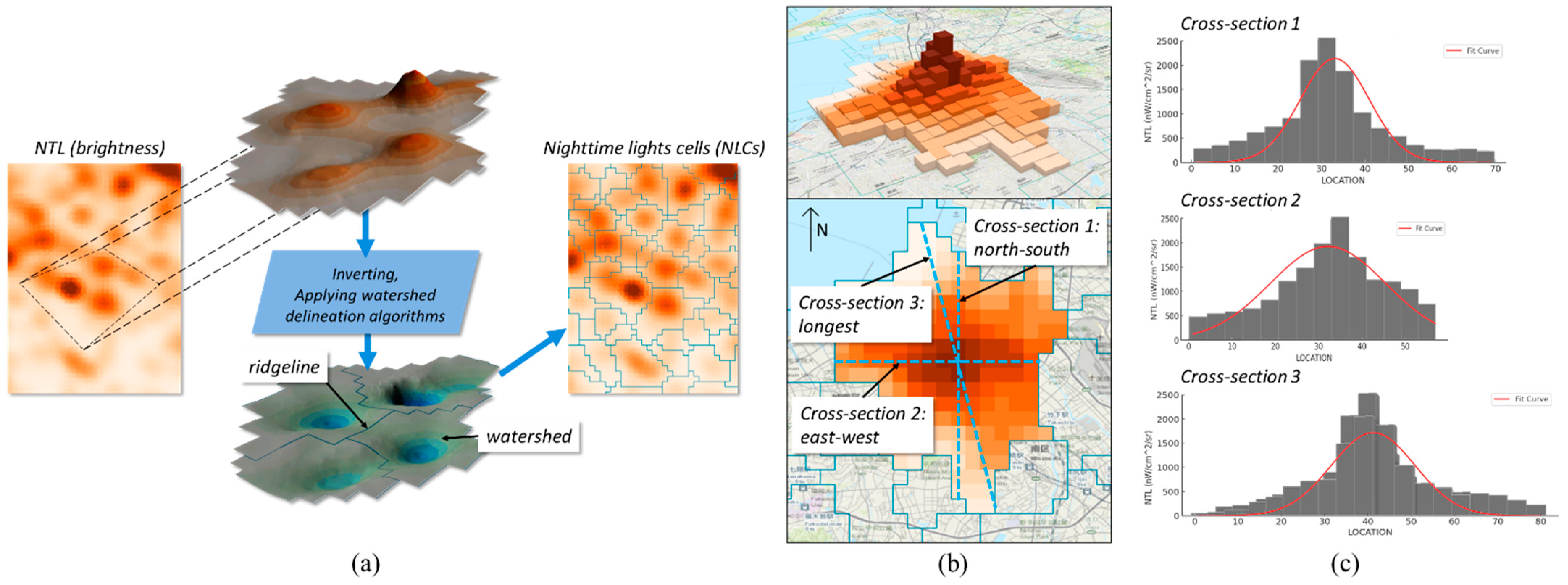
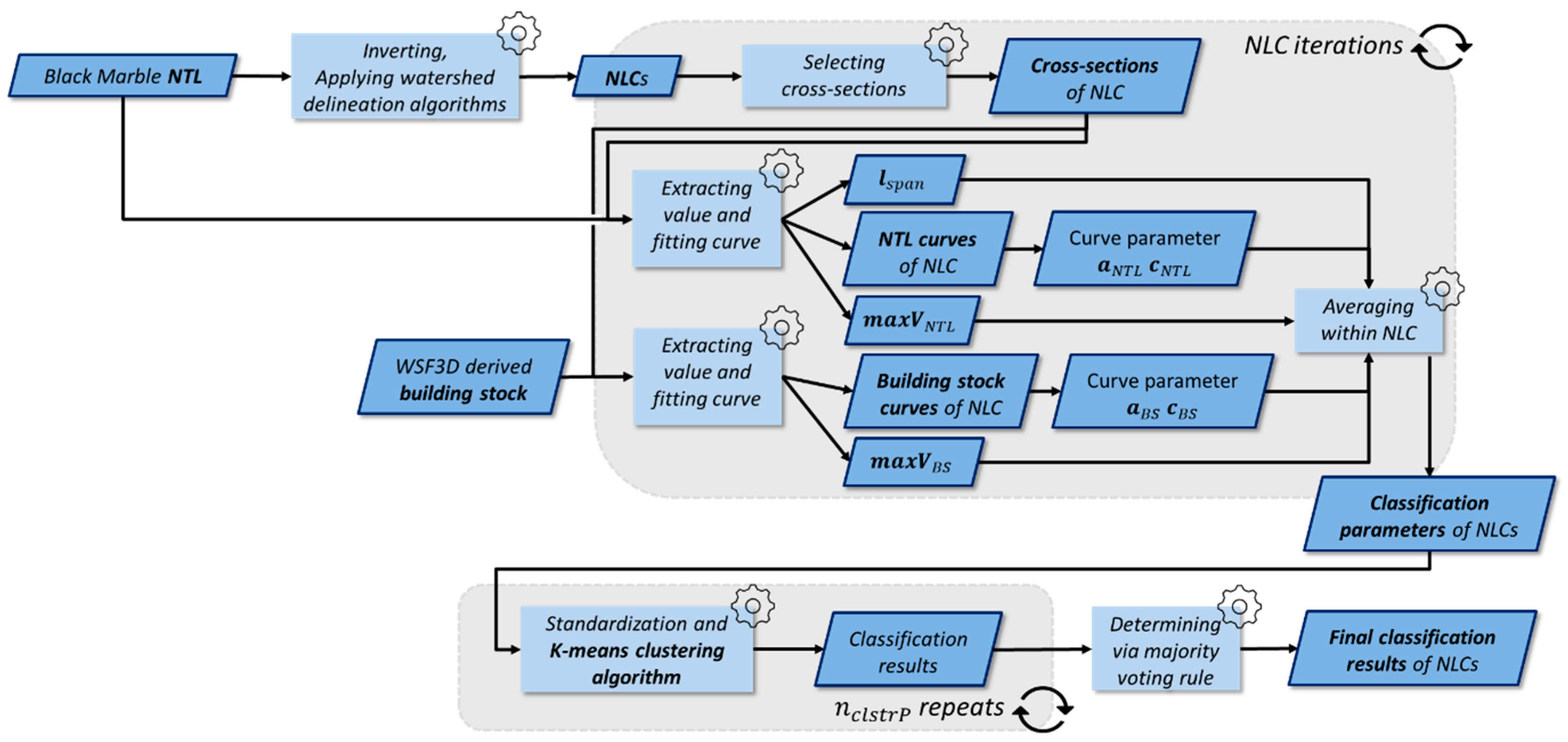
2.2.1. Region Classification Module (RCM)

The objective of BSEEF’s RCM is to distinguish the urban core from other suburban/rural areas. Considering that administrative boundaries may not coincide with the actual extent of urban areas, instead of using administrative units, we opted to use the spatial morphology characteristics of NTL and its similarity to the distribution of building stock as a reference for categorizing and delineating the two types of regions. However, in order to reduce the complexity during characteristic extraction, the basic units of spatial morphological characteristics need to be segmented into dimensions that are close in size with only one vertex value in each unit. Therefore, this study adopted an approach similar to the watershed delineation algorithm commonly used in hydrological analyses, which was first described in Peled and Fishman’s NTL-based study of material stocks in Europe and has also been applied in subsequent studies in other regions [19,65,98]. With the assistance of the SAGA software version 9.0.2 (64 bit), the NTL can be divided into multiple polygons of similar size by inverting (flipping the NTL so that areas with high NTL values are considered as “valleys” and areas with low NTL values are considered as “watershed ridgelines” using a topographical metaphor) and applying watershed delineation algorithms (Figure 1a) [99,100]. Since this step is identical to the one described by Peled and Fishman, we follow their nomenclature and also refer to the delineated polygons as nighttime light cells (NLCs) [19].

With the delineated NLCs, we designed a spatial morphological characteristic extraction method that utilizes the NTL cross-sections within each NLC, as one cross-section is able to provide a relatively accurate representation of the distribution shape of NTLs in a given direction. Considering that NLCs may have different shapes, in order to optimize the computational cost while not missing key characteristics as much as possible, in each NLC, we selected 3 cross-sections oriented in different directions (1. north–south; 2. east–west; 3. longest) and all passing through the vertex pixel with highest NTL value of this NLC (Figure 1b). We then extracted all the pixel values along each cross-section and used these values to fit a curve to obtain the curve parameters (Figure 1c). Here, we assume that the shape of the NTL distribution along the cross-sections is close to the Gaussian function’s bell-shaped curve:

$$f\left(x\right)=a\cdot e^{-\frac{{\left(x-b\right)}^2}{2c^2}} ,$$

(2)

where $a$ is the height of the curve’s peak, $b$ is the position of the peak, and $c$ (Gaussian root-mean-square width or standard deviation) controls the curve width. The average of all curve parameters for the 3 cross-sections was calculated to be used as the NLC classification parameters. However, if different NLCs have similar NTL shapes but different orientations, this can cause the position of the peak to vary with the angle of observation and lead to significant differences during clustering. We, therefore, concluded that the parameter $b$ lacked value for classification purposes and excluded it from the subsequent clustering process. In addition, since the curves are fitted, they may not coincide exactly with the value points on the cross-sections, which may pose another problem, i.e., curve fitting to differently shaped cross-sections from different NLCs may not exclude the possibility of obtaining fitted curves with similar shapes, which may hamper the validity of the classification using the curve parameters. Therefore, as an alternative to the excluded parameter $b$, we added the span length of the longest cross-section ($l_{span}$) and the highest NTL value of this NLC ($max{V}_{NTL}$) as two supplementary parameters for reflecting the shape and size of the cross-sections used to fit curves. The same parameter extraction process was also performed on the distribution of building stock as a reference for checking similarity, resulting in a total of 7 classification parameters: $a_{NTL}$, $c_{NTL}$, $l_{span}$, $max{V}_{NTL}$, $a_{BS}$, $c_{BS}$, and $max{V}_{BS}$.

After extracting the classification parameters, we use an unsupervised approach to classify the NLCs into two clusters based on the parameter similarity between different NLCs. In this step, considering that the cluster count has been determined by the context of this study, we decided to assign each NLC to one of these two pre-determined clusters, excluding the possibility of identifying it as an outlier and assigning it to a new cluster. Therefore, in this step, we adopted the widely used K-means clustering algorithm due to its merits of relative simplicity of implementation, decent performance on large datasets, manual selection of cluster count, and good generalization properties, in contrast to other clustering algorithms, such as density-based spatial clustering of applications with noise (DBSCAN) or agglomerative hierarchical clustering [101,102,103]. However, as the K-means clustering algorithm is sensitive to dataset outliers, which can lead to significant differences in data volume between clusters, in order to minimize such differences and thus alleviate the problem of insufficient samples in the subsequent model training and validation phases, we have also adopted a standardization process prior to executing the K-means clustering algorithm. Finally, in order to improve the robustness of the classification results by minimizing the effects of randomness, we repeated the whole clustering process $n_{clstrP}$ times and determined the final classification results via the majority voting rule [104]. A brief demonstration of the workflow of RCM is shown in Figure 2.

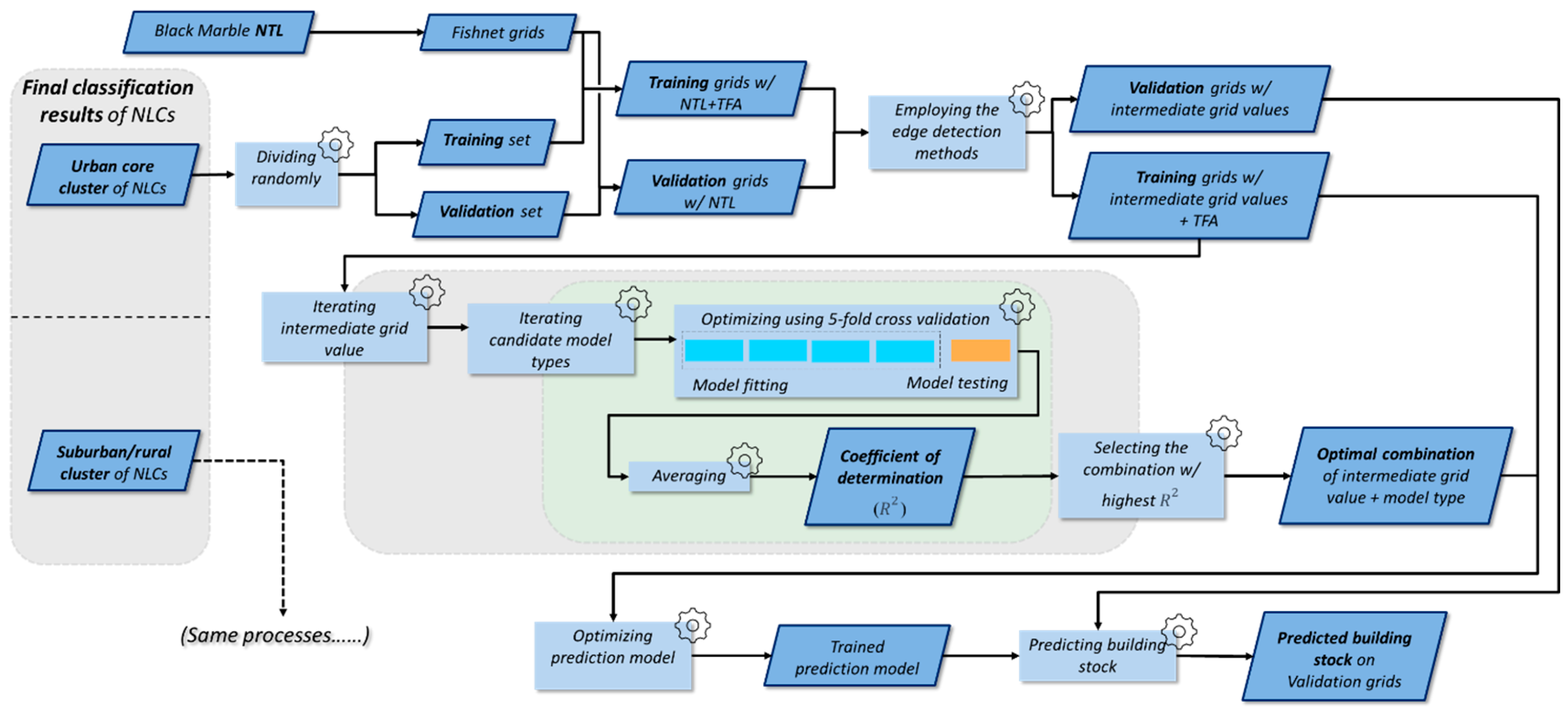
2.2.2. Hybrid Region-Specified Self-Optimization Module (HRSM)

The objective of BSEEF’s HRSM is to screen and identify the optimal model for each area classified by the RCM from a list of candidate models and then train the selected optimal models to obtain region-specific building stock estimates. A brief demonstration of HRSM’s workflow is shown in Figure 3. In the experimental trial using BSEEF, the NLCs within each NLC cluster will be randomly divided into training and validation sets based on a pre-determined ratio ${\theta }_T$, and the fishnet grids delineated by NTL pixel extent will therefore receive a “training” or “validation” label depending on which set they belong to at their location. Each fishnet grid will then obtain an NTL value and a building stock TFA value by inheriting the NTL pixel value and summing the TFA pixel values within its bounds. In addition, inspired by the method of using a moving window to search neighboring pixels for computing the weighted sum in a previous study on eliminating the NTL blooming effect, on the basis of NTL, we also employed the edge detection methods to enhance the connectivity of the neighboring fishnet grids [76]. A series of processed intermediate grid values were obtained and juxtaposed with the original NTL to use as candidate input data for model training, which are shown in Table S1.

With the intermediate grid values and building stock TFA value, the “training” fishnet grids are used in the following model optimization process. Table S2 shows the candidate model types used in this study, which were determined based on a balance of criteria, such as emphasizing variation, reducing computational cost, and code availability. Basically, each intermediate grid value was used for model optimization along with each model type as a grid value–model combination. To evaluate model performance and determine the optimal combination, we adopted a 5-fold cross-validation (CV). In each CV iteration, 4 folds of the “training” fishnet grids were used for preliminary model training, while the remaining 1 fold was used for validation and performance evaluation with a coefficient of determination ($R^2$), as follows:

$$R^2=1-\frac{{{\displaystyle \sum }}_{i=1}^n{\left(y_i-{\widehat{y}}_i\right)}^2}{{{\displaystyle \sum }}_{i=1}^n{\left(y_i-{\overline{y}}_i\right)}^2} ,$$

(3)

where $n$ is the number of samples in the validation fold, $y_i$ is the reference TFA value for the $i$th sample, ${\widehat{y}}_i$ is the predicted TFA value, and ${\overline{y}}_i$ is the average value of the reference TFA. After carrying out all 5 iterations, an average of all 5 $R^2$ values was calculated as the performance score for the current grid value–model combination. Once all combinations have received a performance score, HRSM finds the combination with the highest score and selects it as the optimal combination.

The selected optimal intermediate grid value and building stock TFA values are hereafter used to train and fit an estimation model of the specified optimal type on ‘training’ fishnet grids. The trained estimation model is then applied to the “validation” fishnet grids using the same intermediate grid values for predicting the building stock. Considering that the “validation” fishnet grids only cover $1-{\theta }_T$ portion of the NLCs in each NLC cluster, we repeated HRSM for $n_{HRSM}$ times and performed a spatial-based averaging operation on all the building stock estimation results so that the estimated building stock is able to provide a complete coverage of all the areas of that NLC cluster. By combining the building stock estimation of both NLC clusters, BSEEF’s hybrid region-specified building stock estimation results can hence be obtained.

3. Case Study

The case study area we used in this study to validate BSEEF is Japan. As the mountainous regions account for about three-quarters of its total area, human activities show a highly concentrated pattern, mainly on the scarce plains. Only 5.2% of the total area of Japan (about 1.96 million hectares of the total 37.80 million hectares) is classified as developed land, such as residential and industrial use [105]. A similar concentrated pattern can also be identified on the Black Marble NTL; therefore, we only consider the areas with positive NTL brightness values in this case study. A total of 11161 NLCs have been delineated, with a total area of 11.13 million hectares (29.4% of the total area of Japan), and an average NLC size of 997 hectares. In order to verify whether our BSEEF or one of the stand-alone BSEEF modules can further improve the overall building stock estimation accuracy through NTL, we have designed the following experimental procedures, including trials with side-by-side comparisons using the commonly adopted linear regression-based models. The schematic of the experimental procedures is shown in Figure 4. In order to obtain stable results, avoiding the influence of coincidence, as well as considering the data processing capability of our devices (Ryzen 9 5950X CPU (Advanced Micro Devices, Inc., Santa Clara, CA, USA), DDR4-3200 32GB (16GB×2) F4-3200C16-16GTZRX SDRAM (G.SKILL International Enterprise Co., Ltd., Taipei, China), NVIDIA GeForce RTX 3060 graphics card×2 (Board Manuf. ASUSTeK Computer Inc., Taipei, China)), we set the user-defined parameters to $n_{clstrP}=100$, ${\theta }_T=0.8$ and $n_{HRSM}=330$ to limit the total time cost (approximately 2 h per HRSM run). The average height of each floor ${\overline{h}}_{floor}$ in the case study area was set at 4.1 m with reference to a local commercial building code (Figure S1). To show the differences more intuitively in the results of the trials, we adopt several evaluation indexes, including “Absolute error of total stock ($A{E}_{total}$)” (Equation (4)), “Root mean squared error (RMSE)” (Equation (5)) and “Mean absolute error (MAE)” (Equation (6)), as well as the percentage difference using control trial #3 as a baseline for comparison:

$$A{E}_{total}=\left|{{\displaystyle \sum }}_{i=1}^n{y}_i-{{\displaystyle \sum }}_{i=1}^n{\widehat{y}}_i\right|,$$

(4)

$$RMSE=\sqrt{\frac{1}{n}{{\displaystyle \sum }}_{i=1}^n{\left(y_i-{\widehat{y}}_i\right)}^2},$$

(5)

$$MAE=\frac{1}{n}{{\displaystyle \sum }}_{i=1}^n\left|y_i-{\widehat{y}}_i\right|,$$

(6)

where $n$ in these equations is the sample size of fishnet grids for all of Japan (spatially averaged and merged from all validation sets), $y_i$ is the reference TFA value for the $i$th sample, and ${\widehat{y}}_i$ is the predicted TFA value.

4. Results

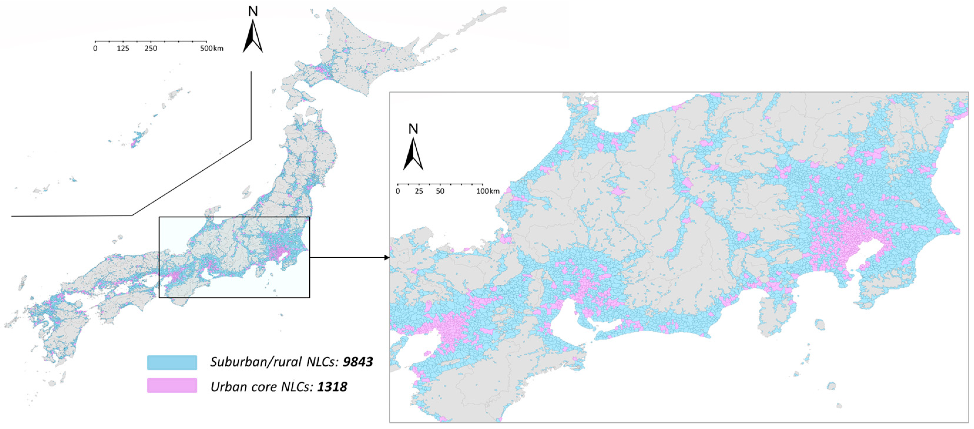
4.1. NLC Classification Results by RCM

In the experimental trial and control trial #1, RCM successfully split all 11161 NLCs into two clusters, including 1318 urban core NLCs and 9843 suburban/rural NLCs. The spatial distributions of the NLCs in these two clusters are shown in Figure 5. The spatial distribution and clustering patterns of urban core NLCs are basically consistent with those of large and medium-sized cities in Japan. For example, the most developed commercial zones in the three major metropolitan areas (Tokyo, Osaka, and Nagoya) and their satellite towns were identified and categorized as urban cores through RCM.

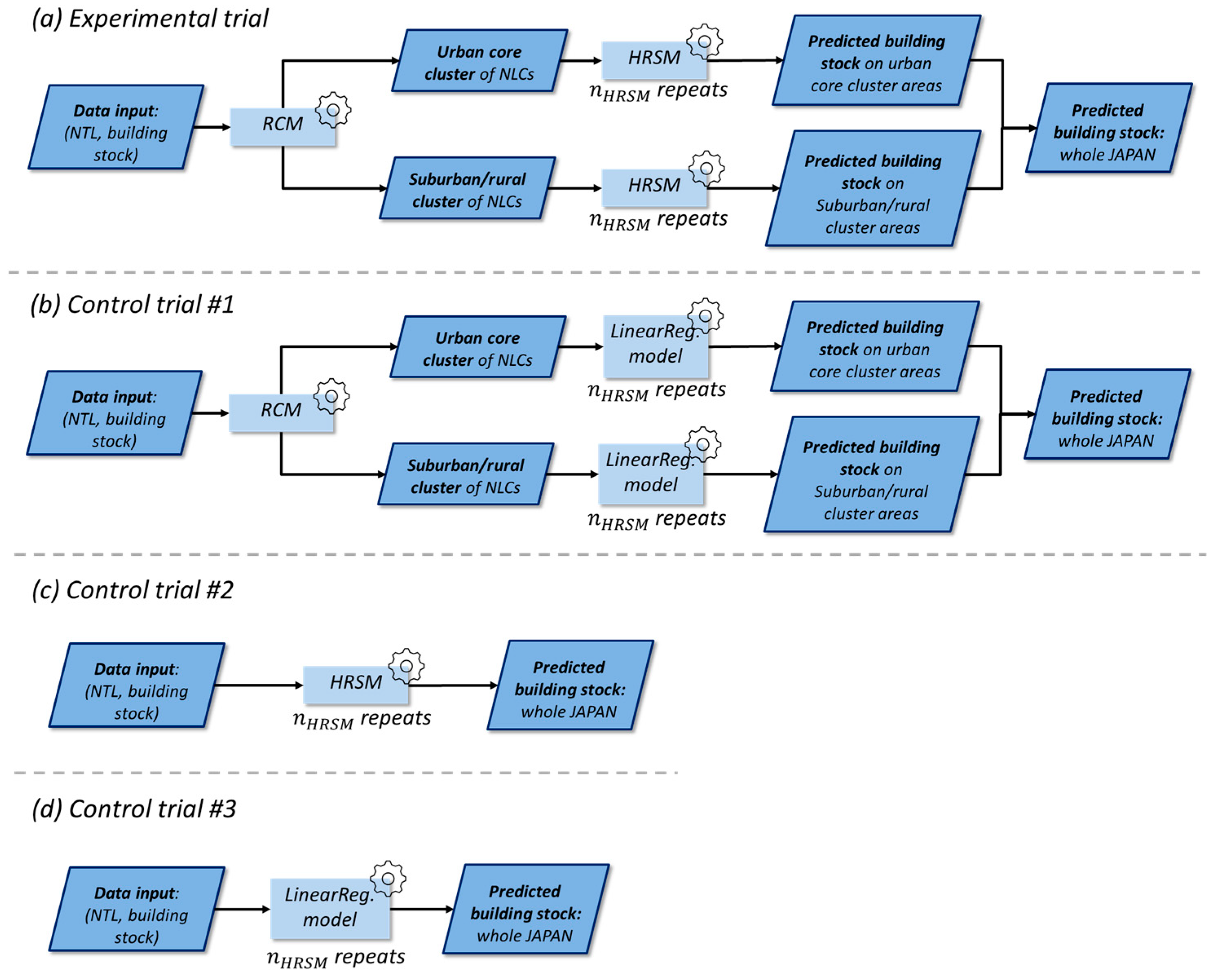
4.2. Building Stock Estimation Results from Experimental and Control Trials

In the experimental trial, for NLCs in the suburban/rural cluster, all 330 repetitions of HRSM selected the gradient boosting regression model type without utilizing any edge detection methods; for NLCs in the urban cluster, the linear regression model type was used in 9 out of 330 repetitions of the HRSM, whereas the gradient-boosted regression model type was selected for all the other repetitions, and no edge detection method was used for all 330 repetitions. In control trial #2, out of the 330 repetitions of HRSM, the multi-layer perceptron regressor model type was used 8 times, while the gradient-boosted regression model type was selected for all other repetitions, and again, edge detection methods were not used for all 330 replications. Table S3 shows the average $R^2$ for the optimized models in all three control trials and the experimental trial, as well as the average $R^2$ by different grid value–model combinations. The building stock estimation results by different trials are shown in

Table 1. The building stock estimation results by different trials, with the percentage difference using control trial #3 as baseline for comparison, reorganized by different regions. (a) Whole Japan (suburban/rural cluster + urban cluster); (b) suburban/rural cluster only; (c) urban cluster only.

(a)
	$\mathrm{Predicted} \mathrm{Building} \mathrm{Stock} \left({\mathrm{m}}^2\right)$	$\mathrm{Absolute} \mathrm{Error} \mathrm{of} \mathrm{Total} \mathrm{Stock} \left(A{E}_{total}\right)$	Root Mean Squared Error (RMSE)	Mean Absolute Error (MAE)
Experimental trial	$9.9457\times {10}^{10}$	$5.9310\times {10}^7$	$2.2968\times {10}^5$	$1.0490\times {10}^5$
		(+16.75%)	(+1.81%)	(+4.81%)
Control trial #1	$9.9481\times {10}^{10}$	$8.3941\times {10}^7$	$2.3378\times {10}^5$	$1.0990\times {10}^5$
		(−17.82%)	(+0.06%)	(+0.28%)
Control trial #2	$9.9424\times {10}^{10}$	$2.6925\times {10}^7$	$2.3022\times {10}^5$	$1.0512\times {10}^5$
		(+62.21%)	(+1.58%)	(+4.62%)
Control trial #3	$9.9469\times {10}^{10}$	$7.1246\times {10}^7$	$2.3392\times {10}^5$	$1.1021\times {10}^5$
Building stock reference (SumTFA)	$9.9397\times {10}^{10}$
(b)
	$\mathrm{Predicted} \mathrm{Building} \mathrm{Stock} \left({\mathrm{m}}^2\right)$	$\mathrm{Absolute} \mathrm{Error} \mathrm{of} \mathrm{Total} \mathrm{Stock} \left(A{E}_{total}\right)$	Root Mean Squared Error (RMSE)	Mean Absolute Error (MAE)
Experimental trial	$5.4710\times {10}^{10}$	$6.2274\times {10}^7$	$1.4428\times {10}^5$	$7.7308\times {10}^4$
		(+95.87%)	(+2.68%)	(+7.19%)
Control trial #1	$5.4703\times {10}^{10}$	$5.5476\times {10}^7$	$1.4818\times {10}^5$	$8.1624\times {10}^4$
		(+96.33%)	(+0.05%)	(+2.00%)
Control trial #2	$5.5625\times {10}^{10}$	$9.7767\times {10}^8$	$1.4508\times {10}^5$	$7.7878\times {10}^4$
		(+35.24%)	(+2.14%)	(+6.50%)
Control trial #3	$5.6157\times {10}^{10}$	$1.5096\times {10}^9$	$1.4826\times {10}^5$	$8.3293\times {10}^4$
Building stock reference (SumTFA)	$5.4647\times {10}^{10}$
(c)
	$\mathrm{Predicted} \mathrm{Building} \mathrm{Stock} \left({\mathrm{m}}^2\right)$	$\mathrm{Absolute} \mathrm{Error} \mathrm{of} \mathrm{total} \mathrm{Stock} \left(A{E}_{total}\right)$	Root Mean Squared Error (RMSE)	Mean Absolute Error (MAE)
Experimental trial	$4.4747\times {10}^{10}$	$2.9645\times {10}^6$	$4.6375\times {10}^5$	$2.4515\times {10}^5$
		(+99.79%)	(+1.37%)	(+0.74%)
Control trial #1	$4.4778\times {10}^{10}$	$2.8465\times {10}^7$	$4.6991\times {10}^5$	$2.5362\times {10}^5$
		(+98.02%)	(+0.06%)	(−2.68%)
Control trial #2	$4.3799\times {10}^{10}$	$9.5075\times {10}^8$	$4.6411\times {10}^5$	$2.4356\times {10}^5$
		(+33.90%)	(+1.30%)	(+1.39%)
Control trial #3	$4.3311\times {10}^{10}$	$1.4384\times {10}^9$	$4.7021\times {10}^5$	$2.4699\times {10}^5$
Building stock reference (SumTFA)	$4.4750\times {10}^{10}$

, which are close in magnitude in terms of the overall results. In addition, the results are also reorganized by different regions (Table 1a: Whole Japan; Table 1b: Suburban/rural cluster NLCs; Table 1c: Urban cluster NLCs) so that the interregional differences in estimation performance can be observed. The results show that the experimental trial has smaller $A{E}_{total}$, RMSE, and MAE values in all regions compared to control trial #3, which indicates that BSEEF is able to improve the accuracy performance of TFA estimation. Moreover, the experimental trial performs better in the suburban/rural cluster than in the urban cluster in terms of RMSE and MAE, whereas the difference in the $A{E}_{total}$ improvement lacks obviousness due to the large magnitude of the reference values in control trial #3.

Control trial #1 and control trial #2 represent the scenario of using stand-alone RCM or HRSM of BSEEF, respectively, in order to verify if there is a specific module primarily contributing to the overall accuracy performance improvement. The results show that control trial #2, using HRSM only, has smaller $A{E}_{total}$, RMSE, and MAE values in all regions compared to control trial #3, which is similar to the results of the experimental trial, but in most cases, the improvement is smaller, suggesting that the use of HRSM alone could not catch up with the performance of full BSEEF. However, in the results of control trial 1, the improvement was not as apparent as in the other trials, with even deterioration in the MAE for the urban cluster and the $A{E}_{total}$ for the whole of Japan observed. This finding suggests that the RCM alone plays a limited role in improving the overall accuracy performance and is less effective than the HRSM.

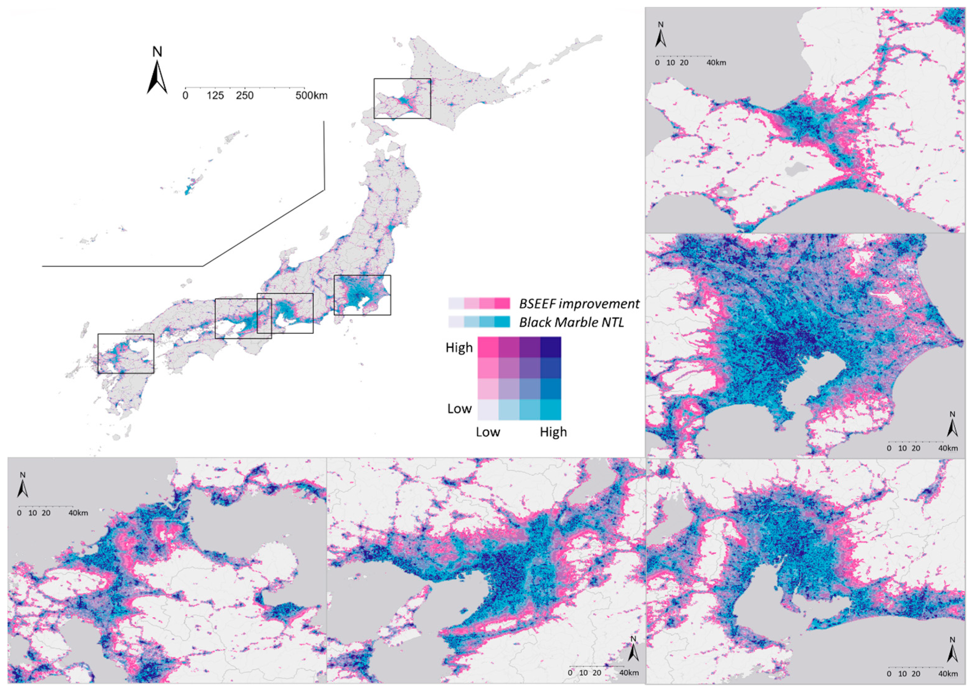
4.3. Spatial Distribution of BSEEF Building Stock Estimation Results

Figure 6a shows the spatial distribution of the building stock predicted by BSEEF. The major metropolitan areas of Japan can be clearly observed from the concentrated areas of building stock, and due to the relatively high spatial resolution, it is possible to identify city subcenters and satellite cities as well. Although this predicted spatial distribution shows a highly similar pattern to that of the reference (Figure S2), in order to further examine the inconsistency between the two distributions, the error in the predicted building stock is also plotted in Figure 6b. In this figure, positive errors representing overestimation are marked in red, while negative errors representing underestimation are marked in blue. Throughout the map, there is more coverage of overestimated areas than underestimated areas, which is consistent with the overestimation trend in the overall results (Table 1a). To better understand the phenomena of over- and underestimation, Figure 6c presents summary pie charts showing the proportion of overestimated and underestimated areas. We established a threshold based on the fishnet grid size to calculate these proportions. Specifically, we set the threshold at 50,000 m², which represents approximately 20–25% of each grid’s area. To account for the need for stricter criteria, we also included half of this threshold (25,000 m²) in the pie charts for a smoother grouping. Across the entire study area, 25.9% of the area is overestimated, while 19.3% is underestimated. In suburban areas, 22.7% is overestimated, and 18.1% is underestimated. In urban areas, overestimation reaches 42.1%, and underestimation is 25.5%. It is clear that the discrepancy in estimation, including both over- and underestimation, which even exceeds two-thirds in urban areas, cannot be ignored.

In addition, the underestimated areas are found mainly in the central parts of metropolitan areas and in small and medium-sized cities with a scattered distribution, while the overestimated areas are primarily located in the urban fringes and suburbs around metropolitan areas, which is also in line with the trends of different regions. However, Hokkaido has an exception in that it overestimates the building stock of decentralized small and medium-sized cities, which may imply that the relationship between NTL and building stock is different here than in other parts of Japan. We also notice that slight overestimations are prevalent in remote rural areas. By simultaneously plotting NTL and building stock reference on a bivariate map (Figure S3), we found that NTL and building stock did not exactly coincide in these areas, as there were illuminated areas that lacked buildings, which may have contributed to the aforementioned overestimation.

To assess the performance of BSEEF in terms of building stock estimation accuracy, we also plot the estimation improvement in BSEEF relative to the basic linear regression model in control trial #3 (Figure 7). The two axes represented in the legend of the bivariate plot represent NTL brightness and BSEEF improvement, respectively. The improvements in BSEEF are mainly distributed in urban core areas (dark blue on the map) and rural/urban fringe areas (dark pink on the map), which implies that our BSEEF is more effective in improving the predictive performance of building stock in these areas compared to linear regression models.

5. Discussion

5.1. Environmental Implications and Opportunities of BSEEF

In the case study of Japan, BSEEF demonstrated that it can noticeably improve the accuracy of building stock estimation using NTL, and this improvement in accuracy can be observed in both urban centers and urban/rural fringes, making BSEEF universally applicable to building stock studies with different study scales and focuses. These more accurate building stock estimations can be further used to foster more refined spatial results related to various environmental and sustainable interests, including circular economy, energy conservation, emission mitigation, waste management, secondary resource recovery, urban planning, and the optimization of resource management strategies [11,106]. Furthermore, in a context where the quality and unavailability of data have emerged as a major impediment to the expansion of studies on built environment stocks [11], BSEEF exhibits less reliance on complex data sources, such as external ancillary data, and necessitates only the use of NTL data and building stock reference data for its modeling processes. Therefore, this characteristic confers a distinct advantage in broadening its application in the field of built environment stock, as it can attain comparatively high accuracy under consistent data source conditions.

As an open framework composed of various sub-modules, the structure of BSEEF is inherently adaptable. It can be customized or progressively refined in response to advances in technology, the specific characteristics of the study area, and the preferences of researchers. This modifiability enables its flexible application across a diverse range of spatial scales and study scopes within built environment stock research. Additionally, it facilitates the integration of potentially applicable cutting-edge technologies and algorithms into these studies, enhancing their breadth and depth. If more advanced datasets become available in the future, the framework can also be accessibly updated based on new data sources to obtain more sophisticated results. For example, considering that NTL typically has a relatively high temporal resolution, the use of dynamic NTL series can facilitate retrospective dynamic built environment stock analyses to identify finer trends and patterns in stock accumulation, support researchers in accurately identifying the underlying drivers behind them, and assist decision makers in authorities to develop appropriate environmental management plans [11,107]. Moreover, BSEEF in this study is not limited to the study of building stock. It also has the potential for modeling, model training, and prediction of any environment and sustainability-related variables (e.g., energy consumption or carbon emissions) that are linked to human activities using NTL within its framework, thus greatly expanding the range of its potential applications.

5.2. Limitations of the BSEEF and Suggestions for Future Improvement

In the process of constructing and applying the BSEEF, we have also identified a number of existing issues and limitations intrinsic to the framework that should be addressed in the future and made some recommendations based on our current understanding of the BSEEF to facilitate more in-depth subsequent research:

• One of the main objectives of developing the BSEEF in this study was to improve the estimation accuracy in urban areas that are susceptible to the saturation effect of NTLs. However, the results did not meet expectations, and the improvement was lower in the urban cluster compared to the suburban cluster. We speculate that this may be due to the clustering setting of the current framework design. To be consistent with the real-world concepts of urban and suburban areas, we categorized all NLCs into two clusters. The suburban cluster consists of NLCs with relatively similar characteristics, while the urban cluster includes all NLCs that are not categorized as suburban. The urban cluster has much greater internal variation, and the current clustering result alone does not adequately reflect these internal differences. This leads to poorer modeling results for urban areas. Theoretically, this problem could be addressed by further subdividing the urban areas into multiple subgroups and fitting a model to each subgroup. However, further subdivision of urban areas is not feasible in practice due to data volume limitations. More subdivisions mean fewer data per group, which may result in insufficient data volume to adequately train the model. Since the urban cluster already has less data volume compared to the suburban cluster, further subdivision for separate model training may result in more accuracy issues. This becomes the most obvious deficiency in the experimental results and needs to be addressed in the future.
• Although BSEEF has a broadly distributed accuracy improvement in predicting building stock in comparison to the fundamental linear regression models, from an overall perspective, the improvement is only a few percentage points per metric. Considering the additional computational cost of using BSEEF, the cost-benefit ratio of obtaining the current improvement in accuracy is not high or even close to marginal. If we had kept the input data types the same and continued to try to iteratively improve the model itself, the costs would likely have continued to increase while the benefits would have gradually diminished. Therefore, in future similar studies, it will be necessary to evaluate the cost of the study and the need for accuracy before executing the entire modeling process. If one is sensitive to computational costs and does not require high predictive accuracy, using a basic linear regression model may be a better choice.
• Some of the errors in the results of this study come from the mismatch between the NTL intensity and the building stock distribution, which is similar to the findings demonstrated in past research on building morphology [108]. With the development of technology and the advancement of observational instruments, the accuracy of the NTL intensity observations is improved, and these mismatches may not simply be categorized as saturation and blooming effects but rather as objective differences. That is, although there is a high correlation between human-induced NTL and building stock, this correlation is not uniformly distributed, and it is weaker in the region of these mismatches. Therefore, the introduction of external ancillary data, such as NDVI, to strengthen the correlation between nighttime lighting and building stock may be necessary to further improve the accuracy [73,74].
• Similarly, due to the existence of differences in the distribution of NTL intensity and building stock, the correlation between these two variables may vary between regions, for example, due to differences in architectural styles or construction standards in different countries or differences in material types or amounts due to different climates, or differences in NTL intensity due to varying levels of economic development and power supply stability. Therefore, when utilizing a single trained BSEEF model for cross-region prediction, differences between regions need to be considered in order to determine the optimal range of applicability of this model. If the similarity between regions cannot be confirmed, further post-prediction verification of the results may be required.
• In this study, the use of the edge detection method in the HRSM module of BSEEF proved to be redundant as the results showed that it did not lead to an improvement in model performance. As this method has been integrated into the model framework process, it adds unnecessary computational cost and weakens the model performance to some extent. A similar situation is likely to occur in future research if more advanced methods are to be incorporated to improve upon the modeling framework of this study. However, trial and error is necessary, and the ensuing computational costs are inevitable.
• One of the main ultimate goals of this study is to enable more convenient snapshot-level building stock estimation, thereby utilizing the high temporal resolution of NTL data to obtain higher temporal resolution maps for the evolution of building stock distribution. Therefore, further experiments are needed after this study to test whether the estimation accuracy of this framework can be reflected at different time scales. If this objective cannot be achieved, further attempts to improve the estimation accuracy are needed.

6. Conclusions

This study explores the possibility of improving existing methods for building stock estimation using remote sensing imagery of NTL. In this study, we designed BSEEF, a novel approach aimed at improving the accuracy of building stock estimation by utilizing NTL images, which can autonomously classify and adaptively optimize models based on regional similarity. The application of BSEEF to a case study in Japan demonstrated its effectiveness in predicting the building stock at a large scale and provided relatively more accurate results, with substantial improvements compared to the traditional linear regression model, especially in the urban core and urban/rural fringe areas that are susceptible to the mismatch between NTL intensity and building stock. BSEEF’s advancement enhances environmental and sustainability research through precise spatial analyses of built environment stocks, offering a flexible, robust framework that adapts easily to technological changes and excels in accuracy without relying heavily on complex datasets. Such advancements would make BSEEF an indispensable tool in strategic urban development planning, fostering sustainable and resilient communities worldwide. Thus, this framework not only addresses current analytical challenges but also sets a foundational methodology for future research endeavors in urban environmental assessments.

References

1. Moomaw, R.L.; Shatter, A.M. Urbanization and Development: A Bias towards Large Cities? J. Urban Econ. 1996, 40, 13–37. [Google Scholar] [CrossRef]
2. Jones, D.W. Urbanization and Energy Use In Economic Development. Energy J. 1989, 10, 29–45. [Google Scholar] [CrossRef]
3. Tang, P.; Huang, J.; Zhou, H.; Fang, C.; Zhan, Y.; Huang, W. Local and telecoupling coordination degree model of urbanization and the eco-environment based on RS and GIS: A case study in the Wuhan urban agglomeration. Sustain. Cities Soc. 2021, 75, 103405. [Google Scholar] [CrossRef]
4. Li, F.; Yigitcanlar, T.; Nepal, M.; Nguyen, K.; Dur, F. Machine learning and remote sensing integration for leveraging urban sustainability: A review and framework. Sustain. Cities Soc. 2023, 96, 104653. [Google Scholar] [CrossRef]
5. Fu, C.; Zhang, Y.; Deng, T.; Daigo, I. The evolution of material stock research: From exploring to rising to hot studies. J. Ind. Ecol. 2022, 26, 462–476. [Google Scholar] [CrossRef]
6. Peng, J.; Pan, Y.; Liu, Y.; Zhao, H.; Wang, Y. Linking ecological degradation risk to identify ecological security patterns in a rapidly urbanizing landscape. Habitat Int. 2018, 71, 110–124. [Google Scholar] [CrossRef]
7. Zhou, Y.; Li, X.; Chen, W.; Meng, L.; Wu, Q.; Gong, P.; Seto, K.C. Satellite mapping of urban built-up heights reveals extreme infrastructure gaps and inequalities in the Global South. Proc. Natl. Acad. Sci. USA 2022, 119, e2214813119. [Google Scholar] [CrossRef]
8. Liang, L.; Wang, Z.; Li, J. The effect of urbanization on environmental pollution in rapidly developing urban agglomerations. J. Clean. Prod. 2019, 237, 117649. [Google Scholar] [CrossRef]
9. Danish; Ulucak, R.; Khan, S.U.D. Determinants of the ecological footprint: Role of renewable energy, natural resources, and urbanization. Sustain. Cities Soc. 2020, 54, 101996. [Google Scholar] [CrossRef]
10. Krausmann, F.; Wiedenhofer, D.; Lauk, C.; Haas, W.; Tanikawa, H.; Fishman, T.; Miatto, A.; Schandl, H.; Haberl, H. Global socioeconomic material stocks rise 23-fold over the 20th century and require half of annual resource use. Proc. Natl. Acad. Sci. USA 2017, 114, 1880–1885. [Google Scholar] [CrossRef]
11. Lanau, M.; Liu, G.; Kral, U.; Wiedenhofer, D.; Keijzer, E.; Yu, C.; Ehlert, C. Taking Stock of Built Environment Stock Studies: Progress and Prospects. Environ. Sci. Technol. 2019, 53, 8499–8515. [Google Scholar] [CrossRef]
12. An, Y.; Chen, T.; Shi, L.; Heng, C.K.; Fan, J. Solar energy potential using GIS-based urban residential environmental data: A case study of Shenzhen, China. Sustain. Cities Soc. 2023, 93, 104547. [Google Scholar] [CrossRef]
13. Dougherty, T.R.; Jain, R.K. Invisible walls: Exploration of microclimate effects on building energy consumption in New York City. Sustain. Cities Soc. 2023, 90, 104364. [Google Scholar] [CrossRef]
14. Tanikawa, H.; Hashimoto, S. Urban stock over time: Spatial material stock analysis using 4d-GIS. Build. Res. Inf. 2009, 37, 483–502. [Google Scholar] [CrossRef]
15. Tanikawa, H.; Fishman, T.; Okuoka, K.; Sugimoto, K. The weight of society over time and space: A comprehensive account of the construction material stock of Japan, 1945–2010. J. Ind. Ecol. 2015, 19, 778–791. [Google Scholar] [CrossRef]
16. Zhang, L.; Plathottam, S.; Reyna, J.; Merket, N.; Sayers, K.; Yang, X.; Reynolds, M.; Parker, A.; Wilson, E.; Fontanini, A.; et al. High-resolution hourly surrogate modeling framework for physics-based large-scale building stock modeling. Sustain. Cities Soc. 2021, 75, 103292. [Google Scholar] [CrossRef]
17. Blázquez, T.; Suárez, R.; Ferrari, S.; Sendra, J.J. Addressing the potential for improvement of urban building stock: A protocol applied to a Mediterranean Spanish case. Sustain. Cities Soc. 2021, 71, 102967. [Google Scholar] [CrossRef]
18. Du, X.; Shen, L.; Wong, S.W.; Meng, C.; Yang, Z. Night-time light data based decoupling relationship analysis between economic growth and carbon emission in 289 Chinese cities. Sustain. Cities Soc. 2021, 73, 103119. [Google Scholar] [CrossRef]
19. Peled, Y.; Fishman, T. Title: Estimation and mapping of the material stocks of buildings of Europe: A novel nighttime lights-based approach. Resour. Conserv. Recycl. 2021, 169, 105509. [Google Scholar] [CrossRef]
20. Guo, J.; Fishman, T.; Wang, Y.; Miatto, A.; Wuyts, W.; Zheng, L.; Wang, H.; Tanikawa, H. Urban development and sustainability challenges chronicled by a century of construction material flows and stocks in Tiexi, China. J. Ind. Ecol. 2021, 25, 162–175. [Google Scholar] [CrossRef]
21. Lanau, M.; Liu, G. Developing an Urban Resource Cadaster for Circular Economy: A Case of Odense, Denmark. Environ. Sci. Technol. 2020, 54, 4675–4685. [Google Scholar] [CrossRef]
22. Mastrucci, A.; Marvuglia, A.; Popovici, E.; Leopold, U.; Benetto, E. Geospatial characterization of building material stocks for the life cycle assessment of end-of-life scenarios at the urban scale. Resour. Conserv. Recycl. 2017, 123, 54–66. [Google Scholar] [CrossRef]
23. Miatto, A.; Schandl, H.; Forlin, L.; Ronzani, F.; Borin, P.; Giordano, A.; Tanikawa, H. A spatial analysis of material stock accumulation and demolition waste potential of buildings: A case study of Padua. Resour. Conserv. Recycl. 2019, 142, 245–256. [Google Scholar] [CrossRef]
24. Miatto, A.; Dawson, D.; Nguyen, P.D.; Kanaoka, K.S.; Tanikawa, H. The urbanisation-environment conflict: Insights from material stock and productivity of transport infrastructure in Hanoi, Vietnam. J. Environ. Manag. 2021, 294, 113007. [Google Scholar] [CrossRef] [PubMed]
25. Kleemann, F.; Lederer, J.; Rechberger, H.; Fellner, J. GIS-based Analysis of Vienna’ s Material Stock in Buildings. J. Ind. Ecol. 2017, 21, 368–380. [Google Scholar] [CrossRef]
26. Tanikawa, H.; Managi, S.; Lwin, C.M. Estimates of Lost Material Stock of Buildings and Roads Due to the Great East Japan Earthquake and Tsunami. J. Ind. Ecol. 2014, 18, 421–431. [Google Scholar] [CrossRef]
27. Mao, R.; Bao, Y.; Huang, Z.; Liu, Q.; Liu, G. High-Resolution Mapping of the Urban Built Environment Stocks in Beijing. Environ. Sci. Technol. 2020, 54, 5345–5355. [Google Scholar] [CrossRef]
28. Wiedenhofer, D.; Baumgart, A.; Matej, S.; Virág, D.; Kalt, G.; Lanau, M.; Tingley, D.D.; Liu, Z.; Guo, J.; Tanikawa, H.; et al. Mapping and modelling global mobility infrastructure stocks, material flows and their embodied greenhouse gas emissions. J. Clean. Prod. 2023, 434, 139742. [Google Scholar] [CrossRef]
29. Ota, Y.; Hiruta, Y.; Yamashita, N.; Shirakawa, H.; Tanikawa, H. Material Stock and Flow Estimation by Identifying the Congruency of Urban Structures between Generations. 2023 Conf. Environ. Inf. Sci. 2023, 37, 195–201. [Google Scholar] [CrossRef]
30. Hu, M. A look at residential building stock in the United States-mapping life cycle embodied carbon emissions and other environmental impact. Sustain. Cities Soc. 2023, 89, 104333. [Google Scholar] [CrossRef]
31. Zhang, N.; Luo, Z.; Liu, Y.; Feng, W.; Zhou, N.; Yang, L. Towards low-carbon cities through building-stock-level carbon emission analysis: A calculating and mapping method. Sustain. Cities Soc. 2022, 78, 103633. [Google Scholar] [CrossRef]
32. Liu, Z.; Saito, R.; Guo, J.; Hirai, C.; Haga, C.; Matsui, T.; Shirakawa, H.; Tanikawa, H. Does Deep Learning Enhance the Estimation for Spatially Explicit Built Environment Stocks through Nighttime Light Data Set? Evidence from Japanese Metropolitans. Environ. Sci. Technol. 2023, 57, 3971–3979. [Google Scholar] [CrossRef] [PubMed]
33. Yu, B.; Deng, S.; Liu, G.; Yang, C.; Chen, Z.; Hill, C.J.; Wu, J. Nighttime Light Images Reveal Spatial-Temporal Dynamics of Global Anthropogenic Resources Accumulation above Ground. Environ. Sci. Technol. 2018, 52, 11520–11527. [Google Scholar] [CrossRef] [PubMed]
34. Esch, T.; Zeidler, J.; Palacios-Lopez, D.; Marconcini, M.; Roth, A.; Mönks, M.; Leutner, B.; Brzoska, E.; Metz-Marconcini, A.; Bachofer, F.; et al. Towards a large-scale 3D modeling of the built environment-joint analysis of tanDEM-X, sentinel-2 and open street map data. Remote Sens. 2020, 12, 2391. [Google Scholar] [CrossRef]
35. Esch, T.; Brzoska, E.; Dech, S.; Leutner, B.; Palacios-Lopez, D.; Metz-Marconcini, A.; Marconcini, M.; Roth, A.; Zeidler, J. World Settlement Footprint 3D-A first three-dimensional survey of the global building stock. Remote Sens. Environ. 2022, 270, 112877. [Google Scholar] [CrossRef]
36. Haberl, H.; Wiedenhofer, D.; Schug, F.; Frantz, D.; Virag, D.; Plutzar, C.; Gruhler, K.; Lederer, J.; Schiller, G.; Fishman, T.; et al. High-Resolution Maps of Material Stocks in Buildings and Infrastructures in Austria and Germany. Environ. Sci. Technol. 2021, 55, 3368–3379. [Google Scholar] [CrossRef] [PubMed]
37. Schug, F.; Frantz, D.; Wiedenhofer, D.; Haberl, H.; Virág, D.; van der Linden, S.; Hostert, P. High-resolution mapping of 33 years of material stock and population growth in Germany using Earth Observation data. J. Ind. Ecol. 2023, 27, 110–124. [Google Scholar] [CrossRef]
38. Levin, N.; Kyba, C.C.M.; Zhang, Q.; Sánchez de Miguel, A.; Román, M.O.; Li, X.; Portnov, B.A.; Molthan, A.L.; Jechow, A.; Miller, S.D.; et al. Remote sensing of night lights: A review and an outlook for the future. Remote Sens. Environ. 2020, 237, 111443. [Google Scholar] [CrossRef]
39. Bao, Y.; Huang, Z.; Wang, H.; Yin, G.; Zhou, X.; Gao, Y. High-resolution quantification of building stock using multi-source remote sensing imagery and deep learning. J. Ind. Ecol. 2023, 27, 350–361. [Google Scholar] [CrossRef]
40. Wu, B.; Huang, H.; Wang, Y.; Shi, S.; Wu, J.; Yu, B. Global spatial patterns between nighttime light intensity and urban building morphology. Int. J. Appl. Earth Obs. Geoinf. 2023, 124, 103495. [Google Scholar] [CrossRef]
41. Wang, G.; Hu, Q.; He, L.; Guo, J.; Huang, J.; Zhong, L. The estimation of building carbon emission using nighttime light images: A comparative study at various spatial scales. Sustain. Cities Soc. 2024, 101, 105066. [Google Scholar] [CrossRef]
42. Zhuo, L.; Ichinose, T.; Zheng, J.; Chen, J.; Shi, P.J.; Li, X. Modelling the population density of China at the pixel level based on DMSP/OLS non-radiance-calibrated night-time light images. Int. J. Remote Sens. 2009, 30, 1003–1018. [Google Scholar] [CrossRef]
43. Bagan, H.; Yamagata, Y. Analysis of urban growth and estimating population density using satellite images of nighttime lights and land-use and population data. GIScience Remote Sens. 2015, 52, 765–780. [Google Scholar] [CrossRef]
44. Anderson, S.J.; Tuttle, B.T.; Powell, R.L.; Sutton, P.C. Characterizing relationships between population density and nighttime imagery for Denver, Colorado: Issues of scale and representation. Int. J. Remote Sens. 2010, 31, 5733–5746. [Google Scholar] [CrossRef]
45. Wang, L.; Fan, H.; Wang, Y. Improving population mapping using Luojia 1-01 nighttime light image and location-based social media data. Sci. Total Environ. 2020, 730, 139148. [Google Scholar] [CrossRef]
46. Mellander, C.; Lobo, J.; Stolarick, K.; Matheson, Z. Night-time light data: A good proxy measure for economic activity? PLoS ONE 2015, 10, e0139779. [Google Scholar] [CrossRef]
47. Doll, C.N.H.; Muller, J.P.; Morley, J.G. Mapping regional economic activity from night-time light satellite imagery. Ecol. Econ. 2006, 57, 75–92. [Google Scholar] [CrossRef]
48. Chen, Z.; Yu, S.; You, X.; Yang, C.; Wang, C.; Lin, J.; Wu, W.; Yu, B. New nighttime light landscape metrics for analyzing urban-rural differentiation in economic development at township: A case study of Fujian province, China. Appl. Geogr. 2023, 150, 102841. [Google Scholar] [CrossRef]
49. Zhang, X.; Cai, Z.; Song, W.; Yang, D. Mapping the spatial-temporal changes in energy consumption-related carbon emissions in the Beijing-Tianjin-Hebei region via nighttime light data. Sustain. Cities Soc. 2023, 94, 104476. [Google Scholar] [CrossRef]
50. Liu, X.; Li, X. Luojia nighttime light data with a 130m spatial resolution providing a better measurement of gridded anthropogenic heat flux than VIIRS. Sustain. Cities Soc. 2023, 94, 104565. [Google Scholar] [CrossRef]
51. Wan, R.; Qian, S.; Ruan, J.; Zhang, L.; Zhang, Z.; Zhu, S.; Jia, M.; Cai, B.; Li, L.; Wu, J.; et al. Modelling monthly-gridded carbon emissions based on nighttime light data. J. Environ. Manag. 2024, 354, 120391. [Google Scholar] [CrossRef] [PubMed]
52. Yang, S.; Yang, X.; Gao, X.; Zhang, J. Spatial and temporal distribution characteristics of carbon emissions and their drivers in shrinking cities in China: Empirical evidence based on the NPP/VIIRS nighttime lighting index. J. Environ. Manag. 2022, 322, 116082. [Google Scholar] [CrossRef]
53. Wang, M.; Wang, Y.; Teng, F.; Ji, Y. The spatiotemporal evolution and impact mechanism of energy consumption carbon emissions in China from 2010 to 2020 by integrating multisource remote sensing data. J. Environ. Manag. 2023, 346, 119054. [Google Scholar] [CrossRef]
54. Wang, M.; Li, R.; Zhang, M.; Chen, L.; Zhang, F.; Huang, C. Mapping high-resolution energy consumption CO2 emissions in China by integrating nighttime lights and point source locations. Sci. Total Environ. 2023, 900, 165829. [Google Scholar] [CrossRef] [PubMed]
55. Guo, W.; Li, Y.; Li, P.; Zhao, X.; Zhang, J. Using a combination of nighttime light and MODIS data to estimate spatiotemporal patterns of CO2 emissions at multiple scales. Sci. Total Environ. 2022, 848, 157630. [Google Scholar] [CrossRef]
56. Han, J.; Meng, X.; Liang, H.; Cao, Z.; Dong, L.; Huang, C. An improved nightlight-based method for modeling urban CO2 emissions. Environ. Model. Softw. 2018, 107, 307–320. [Google Scholar] [CrossRef]
57. Sun, Y.; Wang, S.; Wang, Y. Estimating local-scale urban heat island intensity using nighttime light satellite imageries. Sustain. Cities Soc. 2020, 57, 102125. [Google Scholar] [CrossRef]
58. Liu, Y.; Xu, Y.; Weng, F.; Zhang, F.; Shu, W. Impacts of urban spatial layout and scale on local climate: A case study in Beijing. Sustain. Cities Soc. 2021, 68, 102767. [Google Scholar] [CrossRef]
59. Gong, P.; Li, X.; Wang, J.; Bai, Y.; Chen, B.; Hu, T.; Liu, X.; Xu, B.; Yang, J.; Zhang, W.; et al. Annual maps of global artificial impervious area (GAIA) between 1985 and 2018. Remote Sens. Environ. 2020, 236, 111510. [Google Scholar] [CrossRef]
60. Huang, C.; Zhuang, Q.; Meng, X.; Guo, H.; Han, J. An improved nightlight threshold method for revealing the spatiotemporal dynamics and driving forces of urban expansion in China. J. Environ. Manag. 2021, 289, 112574. [Google Scholar] [CrossRef]
61. Zheng, Y.; He, Y.; Zhou, Q.; Wang, H. Quantitative Evaluation of Urban Expansion using NPP-VIIRS Nighttime Light and Landsat Spectral Data. Sustain. Cities Soc. 2022, 76, 103338. [Google Scholar] [CrossRef]
62. Zhang, Q.; Seto, K.C. Mapping urbanization dynamics at regional and global scales using multi-temporal DMSP/OLS nighttime light data. Remote Sens. Environ. 2011, 115, 2320–2329. [Google Scholar] [CrossRef]
63. Ma, Q.; He, C.; Wu, J.; Liu, Z.; Zhang, Q.; Sun, Z. Quantifying spatiotemporal patterns of urban impervious surfaces in China: An improved assessment using nighttime light data. Landsc. Urban Plan. 2014, 130, 36–49. [Google Scholar] [CrossRef]
64. Huang, X.; Schneider, A.; Friedl, M.A. Mapping sub-pixel urban expansion in China using MODIS and DMSP/OLS nighttime lights. Remote Sens. Environ. 2016, 175, 92–108. [Google Scholar] [CrossRef]
65. Zhao, F.; Wu, H.; Zhu, S.; Zeng, H.; Zhao, Z.; Yang, X.; Zhang, S. Material stock analysis of urban road from nighttime light data based on a bottom-up approach. Environ. Res. 2023, 228, 115902. [Google Scholar] [CrossRef] [PubMed]
66. National Polar Orbiting Operational Environmental Satellite System (NPOESS) Preparatory Project Science Team; National Aeronautics and Space Administration; Earth Observing System Project Science Office. NPP NPOESS Preparatory Project: Building a Bridge to a New Era of Earth Observations. 2011; p. 15. Available online: https://www.nasa.gov/pdf/596329main_NPP_Brochure_ForWeb.pdf (accessed on 25 December 2023).
67. Elvidge, C.D.; Baugh, K.; Zhizhin, M.; Hsu, F.C.; Ghosh, T. VIIRS night-time lights. Int. J. Remote Sens. 2017, 38, 5860–5879. [Google Scholar] [CrossRef]
68. Elvidge, C.D.; Zhizhin, M.; Ghosh, T.; Hsu, F.C.; Taneja, J. Annual time series of global viirs nighttime lights derived from monthly averages: 2012 to 2019. Remote Sens. 2021, 13, 922. [Google Scholar] [CrossRef]
69. Román, M.O.; Wang, Z.; Sun, Q.; Kalb, V.; Miller, S.D.; Molthan, A.; Schultz, L.; Bell, J.; Stokes, E.C.; Pandey, B.; et al. NASA’s Black Marble nighttime lights product suite. Remote Sens. Environ. 2018, 210, 113–143. [Google Scholar] [CrossRef]
70. Levin, N.; Zhang, Q. A global analysis of factors controlling VIIRS nighttime light levels from densely populated areas. Remote Sens. Environ. 2017, 190, 366–382. [Google Scholar] [CrossRef]
71. Zhao, M.; Zhou, Y.; Li, X.; Cao, W.; He, C.; Yu, B.; Li, X.; Elvidge, C.D.; Cheng, W.; Zhou, C. Applications of satellite remote sensing of nighttime light observations: Advances, challenges, and perspectives. Remote Sens. 2019, 11, 1971. [Google Scholar] [CrossRef]
72. Elvidge, C.D.; Cinzano, P.; Pettit, D.R.; Arvesen, J.; Sutton, P.; Small, C.; Nemani, R.; Longcore, T.; Rich, C.; Safran, J.; et al. The nightsat mission concept. Int. J. Remote Sens. 2007, 28, 2645–2670. [Google Scholar] [CrossRef]
73. Zhang, Q.; Schaaf, C.; Seto, K.C. The Vegetation adjusted NTL Urban Index: A new approach to reduce saturation and increase variation in nighttime luminosity. Remote Sens. Environ. 2013, 129, 32–41. [Google Scholar] [CrossRef]
74. Zhuo, L.; Zheng, J.; Zhang, X.; Li, J.; Liu, L. An improved method of night-time light saturation reduction based on EVI. Int. J. Remote Sens. 2015, 36, 4114–4130. [Google Scholar] [CrossRef]
75. Ma, L.; Wu, J.; Li, W.; Peng, J.; Liu, H. Evaluating saturation correction methods for DMSP/OLS nighttime light data: A case study from China’s cities. Remote Sens. 2014, 6, 9853–9872. [Google Scholar] [CrossRef]
76. Cao, X.; Hu, Y.; Zhu, X.; Shi, F.; Zhuo, L.; Chen, J. A simple self-adjusting model for correcting the blooming effects in DMSP-OLS nighttime light images. Remote Sens. Environ. 2019, 224, 401–411. [Google Scholar] [CrossRef]
77. Luo, Z.; Wu, Y.; Zhou, L.; Sun, Q.; Yu, X.; Zhu, L.; Zhang, X.; Fang, Q.; Yang, X.; Yang, J.; et al. Trade-off between vegetation CO2 sequestration and fossil fuel-related CO2 emissions: A case study of the Guangdong–Hong Kong–Macao Greater Bay Area of China. Sustain. Cities Soc. 2021, 74, 103195. [Google Scholar] [CrossRef]
78. Liu, Z.; Liu, S. Urban shrinkage in a developing context: Rethinking China’s present and future trends. Sustain. Cities Soc. 2022, 80, 103779. [Google Scholar] [CrossRef]
79. Hao, R.; Yu, D.; Sun, Y.; Cao, Q.; Liu, Y.; Liu, Y. Integrating multiple source data to enhance variation and weaken the blooming effect of DMSP-OLS light. Remote Sens. 2015, 7, 1422–1440. [Google Scholar] [CrossRef]
80. Okujeni, A.; van der Linden, S.; Jakimow, B.; Rabe, A.; Verrelst, J.; Hostert, P. A comparison of advanced regression algorithms for quantifying urban land cover. Remote Sens. 2014, 6, 6324–6346. [Google Scholar] [CrossRef]
81. Frantz, D.; Schug, F.; Okujeni, A.; Navacchi, C.; Wagner, W.; van der Linden, S.; Hostert, P. National-scale mapping of building height using Sentinel-1 and Sentinel-2 time series. Remote Sens. Environ. 2021, 252, 112128. [Google Scholar] [CrossRef]
82. Zhang, R.; Yamashita, N.; Liu, Z.; Guo, J.; Hiruta, Y.; Shirakawa, H.; Tanikawa, H. Paving the way to the future: Mapping historical patterns and future trends of road material stock in Japan. Sci. Total Environ. 2023, 903, 166632. [Google Scholar] [CrossRef]
83. Georganos, S.; Grippa, T.; Vanhuysse, S.; Lennert, M.; Shimoni, M.; Wolff, E. Very High Resolution Object-Based Land Use-Land Cover Urban Classification Using Extreme Gradient Boosting. IEEE Geosci. Remote Sens. Lett. 2018, 15, 607–611. [Google Scholar] [CrossRef]
84. Touzani, S.; Granderson, J.; Fernandes, S. Gradient boosting machine for modeling the energy consumption of commercial buildings. Energy Build. 2018, 158, 1533–1543. [Google Scholar] [CrossRef]
85. Xu, Y.; Li, F.; Asgari, A. Prediction and optimization of heating and cooling loads in a residential building based on multi-layer perceptron neural network and different optimization algorithms. Energy 2022, 240, 122692. [Google Scholar] [CrossRef]
86. Tan, X.; Zhu, X.; Chen, J.; Chen, R. Modeling the direction and magnitude of angular effects in nighttime light remote sensing. Remote Sens. Environ. 2022, 269, 112834. [Google Scholar] [CrossRef]
87. Zheng, Q.; Weng, Q.; Zhou, Y.; Dong, B. Impact of temporal compositing on nighttime light data and its applications. Remote Sens. Environ. 2022, 274, 113016. [Google Scholar] [CrossRef]
88. Wang, Z.; Román, M.O.; Kalb, V.L.; Miller, S.D.; Zhang, J.; Shrestha, R.M. Quantifying uncertainties in nighttime light retrievals from Suomi-NPP and NOAA-20 VIIRS Day/Night Band data. Remote Sens. Environ. 2021, 263, 112557. [Google Scholar] [CrossRef]
89. Hao, X.; Liu, J.; Heiskanen, J.; Maeda, E.E.; Gao, S.; Hao, X.; Liu, J.; Heiskanen, J.; Eiji, E.; Gao, S.; et al. A robust gap-filling method for predicting missing observations in daily Black Marble nighttime light data A robust gap-filling method for predicting missing observations in daily Black. GIScience Remote Sens. 2023, 60, 2282238. [Google Scholar] [CrossRef]
90. NASA Level 1 and Atmosphere Archive and Distribution System Distributed Active Archive Center. NASA VIIRS Land Science Investigator-Led Processing System. VNP46A4-VIIRS/NPP Lunar BRDF-Adjusted Nighttime Lights Yearly L3 Global 15 arc second Linear Lat Lon Grid. 2021. Available online: https://ladsweb.modaps.eosdis.nasa.gov/missions-and-measurements/products/VNP46A4/#overview (accessed on 28 January 2024).
91. Wang, Z.; Shrestha, R.M.; Roman, M.O.; Kalb, V.L. NASA’s Black Marble Multiangle Nighttime Lights Temporal Composites. IEEE Geosci. Remote Sens. Lett. 2022, 19, 2505105. [Google Scholar] [CrossRef]
92. Liu, M.; Ma, J.; Zhou, R.; Li, C.; Li, D.; Hu, Y. High-resolution mapping of mainland China’s urban floor area. Landsc. Urban Plan. 2021, 214, 104187. [Google Scholar] [CrossRef]
93. Heeren, N.; Hellweg, S. Tracking Construction Material over Space and Time: Prospective and Geo-referenced Modeling of Building Stocks and Construction Material Flows. J. Ind. Ecol. 2019, 23, 253–267. [Google Scholar] [CrossRef]
94. Müller, D.B. Stock dynamics for forecasting material flows-Case study for housing in The Netherlands Dynamic modelling Prospects for resource demand Waste management Vintage effects Diffusion processes. Ecol. Econ. 2005, 9, 142–156. [Google Scholar] [CrossRef]
95. Brady, L.; Abdellatif, M. Assessment of energy consumption in existing buildings. Energy Build. 2017, 149, 142–150. [Google Scholar] [CrossRef]
96. Guo, J.; Miatto, A.; Shi, F.; Tanikawa, H. Spatially explicit material stock analysis of buildings in Eastern China metropoles. Resour. Conserv. Recycl. 2019, 146, 45–54. [Google Scholar] [CrossRef]
97. Pérez-Lombard, L.; Ortiz, J.; Pout, C. A review on buildings energy consumption information. Energy Build. 2008, 40, 394–398. [Google Scholar] [CrossRef]
98. Liang, H.; Bian, X.; Dong, L. Towards net zero carbon buildings: Accounting the building embodied carbon and life cycle-based policy design for Greater Bay Area, China. Geosci. Front. 2024, 15, 101760. [Google Scholar] [CrossRef]
99. Conrad, O.; Bechtel, B.; Bock, M.; Dietrich, H.; Fischer, E.; Gerlitz, L.; Wehberg, J.; Wichmann, V.; Böhner, J. System for Automated Geoscientific Analyses (SAGA) v. 2.1.4. Geosci. Model Dev. 2015, 8, 1991–2007. [Google Scholar] [CrossRef]
100. Chen, Z.; Yu, B.; Song, W.; Liu, H.; Wu, Q.; Shi, K.; Wu, J. A New Approach for Detecting Urban Centers and Their Spatial Structure with Nighttime Light Remote Sensing. IEEE Trans. Geosci. Remote Sens. 2017, 55, 6305–6319. [Google Scholar] [CrossRef]
101. Kanungo, T.; Mount, D.M.; Netanyahu, N.S.; Piatko, C.D.; Silverman, R.; Wu, A.Y. An Efficient k-Means Clustering Algorithm: Analysis and Implementation. IEEE Trans. Pattern Anal. Mach. Intell. 2002, 24, 881–892. [Google Scholar] [CrossRef]
102. Jain, A.K. Data clustering: 50 years beyond K-means. Pattern Recognit. Lett. 2010, 31, 651–666. [Google Scholar] [CrossRef]
103. Google for Developers. K-Means Advantages and Disadvantages. Machine Learning, Advanced Courses, Clustering. 2022. Available online: https://developers.google.com/machine-learning/clustering/algorithm/advantages-disadvantages (accessed on 4 February 2024).
104. Ballabio, D.; Todeschini, R.; Consonni, V. Recent Advances in High-Level Fusion Methods to Classify Multiple Analytical Chemical Data. Data Handl. Sci. Technol. 2019, 31, 129–155. [Google Scholar] [CrossRef]
105. Statistics Bureau, Ministry of Internal Affairs and Communications, Japan. Statistical Handbook of Japan 2022. 2022. Available online: https://www.stat.go.jp/english/data/handbook/pdf/2020all.pdf (accessed on 28 February 2024).
106. Wang, K.; Aktas, Y.D.; Malki-Epshtein, L.; Wu, D.; Ammar Bin Abdullah, M.F. Mapping the city scale anthropogenic heat emissions from buildings in Kuala Lumpur through a top-down and a bottom-up approach. Sustain. Cities Soc. 2022, 76, 103443. [Google Scholar] [CrossRef]
107. Kapur, A.; Keoleian, G.; Kendall, A.; Kesler, S.E. Dynamic modeling of in-use cement stocks in the United States. J. Ind. Ecol. 2008, 12, 539–556. [Google Scholar] [CrossRef]
108. Xu, G.; Su, J.; Xia, C.; Li, X.; Xiao, R. Spatial mismatches between nighttime light intensity and building morphology in Shanghai, China. Sustain. Cities Soc. 2022, 81, 103851. [Google Scholar] [CrossRef]
Figure 1. (a) A schematic demonstration of the division of nighttime light cells (NLCs) with watershed delineation algorithms. (b) The selection of 3 cross-sections orienting in different directions. (c) Pixel value extraction along each cross-section and curve fitting.
Remotesensing 16 02495 g001
Figure 2. A schematic demonstration of the workflow of RCM.
Remotesensing 16 02495 g002
Figure 3. A schematic demonstration of the workflow of HRSM.
Remotesensing 16 02495 g003
Figure 4. A schematic of the experimental procedures in the case study, including (a) experimental trial with both RCM and HRSM applied; (b) control trial #1 with RCM applied but without HRSM; (c) control trial #2 with HRSM applied but without RCM; and (d) control trial #3 with neither RCM nor HRSM applied.
Remotesensing 16 02495 g004
Figure 5. Spatial distribution of suburban/rural NLCs and urban core NLCs throughout Japan, including zoomed-in maps of the major metropolitan areas.
Remotesensing 16 02495 g005
Figure 6. (a) Spatial distribution of BSEEF predicted building stock results. (b) Error in the predicted building stock. (c) Pie charts with proportions of overestimated and underestimated areas in different regions.
Remotesensing 16 02495 g006aRemotesensing 16 02495 g006bRemotesensing 16 02495 g006c
Figure 7. Spatial distribution of BSEEF estimation improvement over the basic linear regression model.
Remotesensing 16 02495 g007