Abstract
In this paper, a technology named SCM−ANN combining physical scattering mechanisms and artificial intelligence is proposed to realize radar cross-section (RCS) extrapolation of non-cooperative conductor targets with higher efficiency. Firstly, an adaptive scattering center (SC) extraction algorithm is used to construct the scattering center model (SCM) for non-cooperative targets from radar echoes in the low-frequency band (LFB). Secondly, an artificial neural network (ANN) is constructed to capture the nonlinear relationship between the real LFB echoes and those reconstructed from the SCM. Finally, the SCM is used to reconstruct echoes in the high-frequency band (HFB), and these reconstructions, together with the trained ANN, optimize the extrapolated HFB RCS. For the SCM−ANN technology, physical mechanistic modes are used for trend prediction, and artificial intelligence is used for regression optimization based on trend prediction. Simulation results show that the proposed method can achieve a 50% frequency extrapolation range, with an average prediction error reduction of up to 40% compared with the traditional scheme. By incorporating physical mechanisms, this proposed approach offers improved accuracy and an extended extrapolation range compared with the RCS extrapolation techniques relying solely on numerical prediction.
1. Introduction
Automatic Target Recognition (ATR) technology based on target characteristic databases has been increasingly applied in the field of national defense and security [1,2]. The typical approach involves comparing the radar echoes of a target with those stored in the database and improving the radar’s recognition rate and tracking capability through the similarity with the template. However, constructing such a target characteristic database demands massive computational resources and time due to the intensive sampling that must be performed in the frequency and angular domains. In such a context, efficiently acquiring target features becomes one of the most critical considerations.
Many techniques have been developed focusing on accelerating the process of acquiring target scattering characteristics, which can be generally divided into algorithmic acceleration and numerical prediction. In terms of algorithm acceleration, high-frequency algorithms [3], hybrid algorithms [4], and parallel techniques [5] have been intensively studied and widely used as representative schemes. For example, high-frequency methods such as Shooting and Bouncing Ray (SBR) [6] and Physical Optics (PO) [7] are considered to be preferred solutions for quickly solving the scattering characteristics of electrically large targets. Several studies have shown that the algorithm efficiency can be further enhanced by operating ray tubes [8], constructing tree structures [9,10], and parallel computing. However, these methods remain resource-intensive in terms of time and resource consumption, particularly when dealing with the computation of a large number of entries during intensive sampling. In contrast, numerical prediction techniques achieve accelerated computation mainly by reducing the number of simulations [11,12], which mainly include angular domain interpolation and frequency domain extrapolation. In particular, artificial intelligence is regarded as a special kind of predictive technology that is favored by researchers due to its excellent nonlinear representation. For example, Chen [13] applied machine learning technology to solve the polarized bistatic scattering characteristics from a finite medium cylinder. Xiao [14] developed a hybrid model incorporating PO, support vector regression, and experimental design for analyzing the monostatic RCS of a conducting target. Jacobs and Du Plessis [15] established a Gaussian process regression to predict the electromagnetic response of radar targets. It cannot be ignored that the prediction accuracy of such techniques is overly dependent on the training samples. The prediction effect will be greatly reduced when the training samples have low similarity, which will lead to a limited frequency extrapolation range, weak broadband prediction, etc. Considering the limitations of the above solutions, it is necessary to develop new technologies.
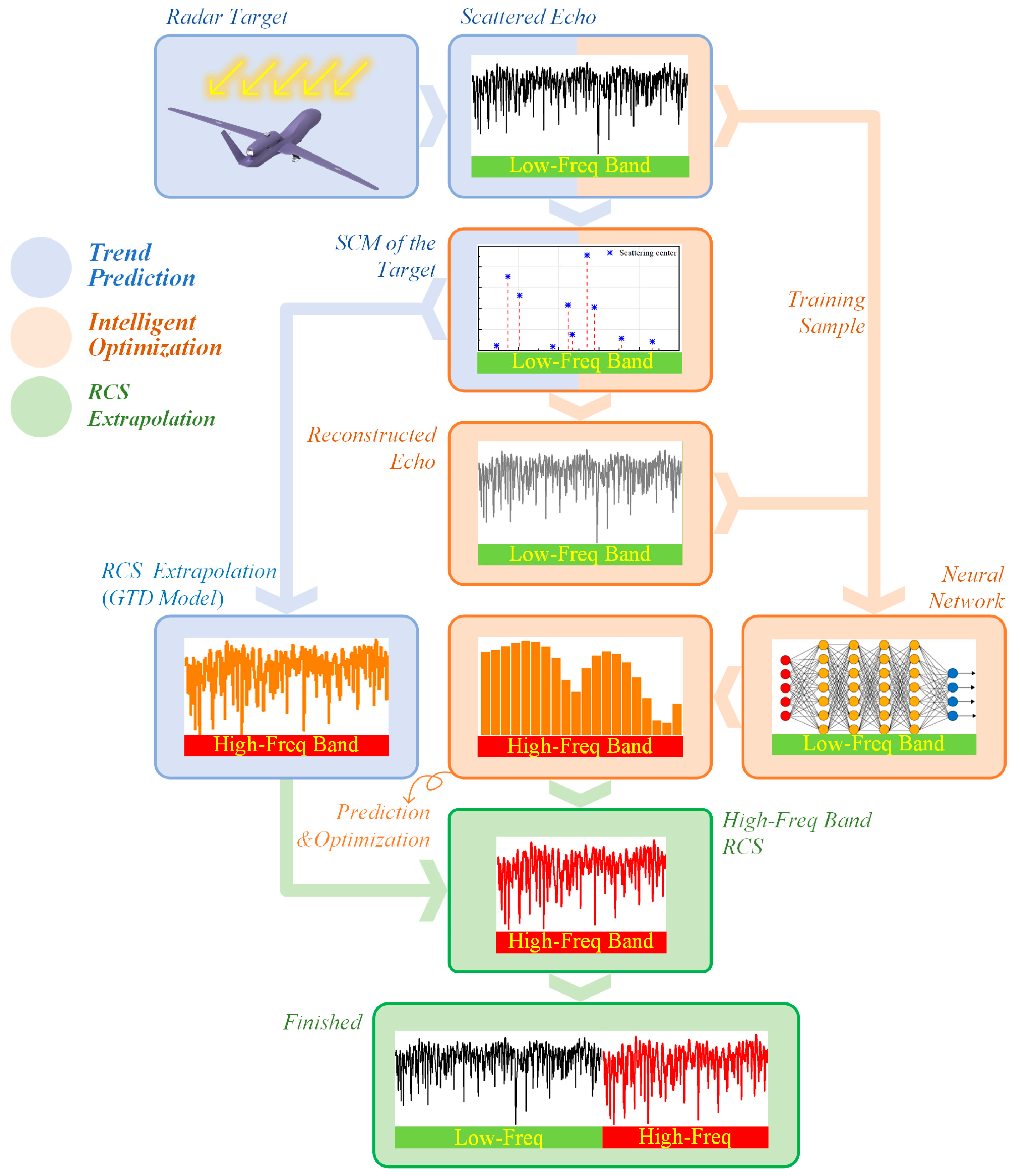
In this paper, an RCS extrapolation technology (named SCM−ANN) based on SCM and ANN is proposed to further improve the prediction effect of target scattering characteristics. The significant difference between the developed method and the proposed method is that the proposed method provides trend prediction guided by physical mechanisms to improve the limitations present in numerical prediction. Certainly, it is feasible and beneficial to incorporate physical mechanisms as a priori information into artificial intelligence, which has become the consensus of many scholars [16,17]. The schematic of SCM−ANN is shown in Figure 1. As depicted in Figure 1, the proposed method is structured into three key sections, each represented by a distinct color: trend prediction (blue), intelligent optimization (orange), and RCS extrapolation (green). In the trend prediction section, the primary objective is to develop the SCM in the LFB and predict the trend of HFB echoes by leveraging the established SCM. Within the framework of SCM−ANN technology, an adaptive parameter estimation method is employed to formulate the parameterized model of the target from an inverse perspective. In contrast to forward modeling methods [18,19], the proposed method estimates the SC [20,21,22] of the target directly from the scattered echoes without requiring knowledge of the target’s geometrical structures. Furthermore, compared to previous work [23,24] that requires the number of SCs as an antecedent input parameter, the proposed method enables the estimation of the number of SCs. This means that the proposed SCM−ANN technology is particularly suitable for non-cooperative targets. It should be noted that the trend prediction is based on the basic approximation that the SCM will remain relatively stable when the incident frequency changes slightly. In the intelligent optimization section, the core goal is to construct a mapping network between reconstructed echoes and real echoes using ANN [25,26] to reduce errors introduced by the trend prediction stage. In contrast to existing works, the SCM-ANN technology achieves RCS extrapolation solely based on LFB echoes. This provides a viable solution for acquiring scattering echoes in frequency bands that are challenging to measure due to constraints such as time, cost, or hardware limitations. Furthermore, the proposed method demonstrates an enhanced capability to address complex targets, attributed to its more precise trend prediction, which is derived from the physical mechanism and surpasses predictions obtained through purely numerical training. The SCM-ANN technology exhibits a wide applicability range that can effectively handle echoes obtained from measurements, EM simulations, and GTD models. Both simulation and real measurement results validate this perspective. The innovative aspects of this paper include the following: (1) an RCS extrapolation technique called SCM−ANN is proposed for non-cooperative targets; (2) the SCM of the target is adaptively constructed, which is further utilized for trend prediction in the RCS extrapolated bands; (3) an ANN incorporating physical mechanisms is developed, and the trend prediction is used as a priori information to improve the prediction accuracy of the network; and (4) the use of numerical simulation and measurement results to validate the effectiveness of the proposed method.
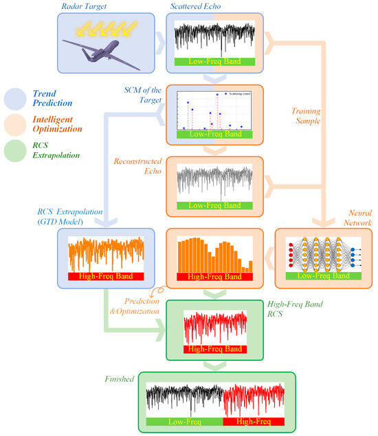
Figure 1.
Schematic representation of SCM−ANN.
The rest of the paper is organized as follows: In Section 2, the SCM of the target is established, and the trend prediction of extrapolation bands based on GTD is proposed. In Section 3, an intelligent optimization network based on ANN is established to reduce the prediction error. In Section 4, simulation and measurement results are used to validate the effectiveness of SCM−ANN. Section 5 discusses the advantages and limitations of SCM−ANN technology. Finally, Section 6 is devoted to the conclusions of this paper.
2. Construction of SCM Based on Radar Echoes
2.1. Acquisition of Target Scattering Echoes
SBR is one of the most powerful solutions for obtaining electromagnetic scattering echoes from electrically large targets since it has excellent computational accuracy and clear physical concepts. By integrating the backward ray tracing acceleration technique into SBR, an improved SBR-PO/PTD algorithm is proposed [27], and the efficiency of echo acquisition is further enhanced while maintaining accuracy. The improved SBR-PO/PTD algorithm is structured into three steps: ray path tracing, ray field strength tracing, and far-field integration. Initially, a series of ray tubes are employed to simulate the incidence of electromagnetic waves upon the target surface. Subsequently, geometrical optics [28] is used to model the multiple reflections of the ray tubes as they interact with the target surface. Finally, the PO and PTD are introduced to solve for the scattered field when the ray tubes depart from the object’s surface. In the execution of the algorithm, the target is discretized into a large number of triangular patches.
As shown in (1), the total scattered field can be obtained by the vector superposition of the PO-generated scattered component contributed by each triangular patch and the PTD-generated diffracted component contributed by the edges.
where ; ; and is the diffraction field of the edges. The number of triangular patches is denoted by . is defined as the unit vector in the scattering direction, is the current density, and is the distance from the triangle patch to the observation point. and are as follows:
where and denote the incident electric and magnetic fields, respectively. is the angle between the incident direction and the edge; represents the angle between the scattering direction and the edge. is the tangent vector of the edge. , , and represent the diffraction coefficient; η represents the spatial wave impedance.
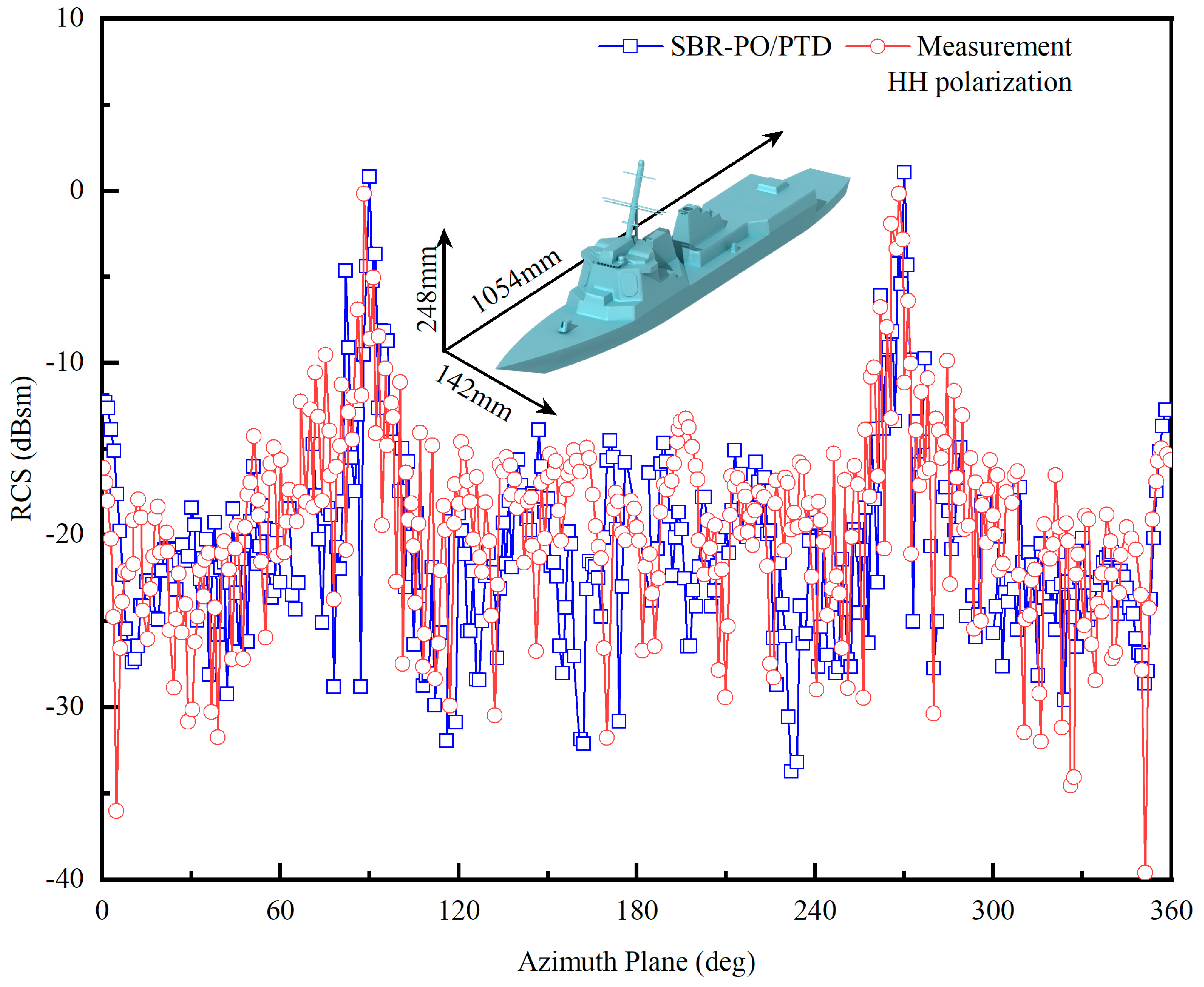
The accuracy and validity of the improved SBR-PO/PTD method are evaluated in this example to ensure the accuracy of the generated target echoes used in the following SCM constructions. The RCS of a PEC ship model (1054 mm × 142 mm × 248 mm) derived from the improved SBR-PO/PTD method is compared with the measurement result in [29], as shown in Figure 2. The ship model has 75,290 patches. The incident frequency is set to 10 GHz, and the simulation results are basically consistent with the measurement data, indicating that SBR-PO/PTD is a suitable strategy for acquiring target echoes.

Figure 2.
SBR-PO/PTD algorithm validation.
In the follow-up process, the radar echoes generated by the SBR-PO/PTD method are further utilized to construct the SCM of the target. Based on the consideration of real-time and echo analysis, the SCM constructed in this work is one-dimensional (2D and 3D SCM are mostly used for image processing).
2.2. Parameter Extraction of SCs
- Mathematical model of SCs
In the optical region of a radar, the scattered field of the target can be effectively modified as the sum of the scattering contributions arising from multiple strong scattering points (also called SCs). Many mathematical models have been established to describe the frequency domain scattering characteristics of individual SCs, such as the ideal point model, the GTD model, and the attribute scattering center model. The ideal point model assumes that the scattering characteristics of each SC remain invariant with respect to both frequency and incidence angle. This model is simple in form but fails to comprehensively capture the full scattering laws of complex targets. The attributed scattering center model extends the traditional notion of “scattering point” by introducing the description of distributed scattering sources. Such methods pull into additional parameters such as geometry and orientation, which, however, pose challenges for the direct extraction of echoes from non-cooperative targets. The GTD model establishes a direct correlation between the frequency dependence factor and the power exponent, wherein the value of the latter depends on the particular scattering structure (as shown in Table 1). This ensures that the GTD model possesses a clear physical meaning. Consequently, the GTD is used to construct the SCM of the targets in this paper with the corresponding radar echo represented in (1).

Table 1.
Typical values of scattering structure.
In (3), represents the number of SCs, and is the amplitude of the SC. represents the step frequency, is the starting frequency of the radar pulse for each operating cycle, is the frequency hopping interval, and is the number of frequency steps, then we have . is defined as the position of the SC relative to the origin of the phase reference. denotes the type of the SC. is the speed of light, and represents the additive complex Gaussian white noise. In this way, the SCM can be completely described by the parameter set .
The presence of exponential and power functions in (3) makes it necessary to reformulate the equation to satisfy the requirements of the spectral estimation model before feature extraction.
Perform a Taylor series expansion at , one can obtain the following:
Perform the binomial expansion for :
Comparing (4) and (5), under the condition of , higher-order terms can be ignored:
Radar echoes are approximately written in a form consistent with spectral estimation techniques [30,31,32]:
in which
Next, the SC parameters can be extracted from the echoes according to the adaptive TLS-ESPRIT algorithm [33].
- B.
- Estimating the position and type of SCs
In the adaptive TLS-ESPRIT algorithm, the eigenvalues are solved by performing a singular value decomposition on . Let :
Next, construct the 1D echo data into a matrix with Hankel form, in which .
Calculate the autocorrelation and cross-correlation matrices of formulas and , denoted as and . Perform singular value decomposition on .
Obviously, , , and correspond to the signal subspace; , , and correspond to the noise subspace. The eigenvalues of the signal subspace can be solved, and the detailed steps can be referred to [33]. Further, the position of the SCs can be determined by (15). By dissecting the approximation obtained for (16) according to Table 1, the type of SC can be determined.
- C.
- Extracting the amplitude of the SCs
The amplitude of the SCs is obtained by a least squares solution [34], using the type and location of the identified SCs by (15) and (16), where is the 1D vector form consisting of the echo signal . The matrix is the amplitude to be solved of the SCs.
- D.
- Simulation examples based on the GTD model
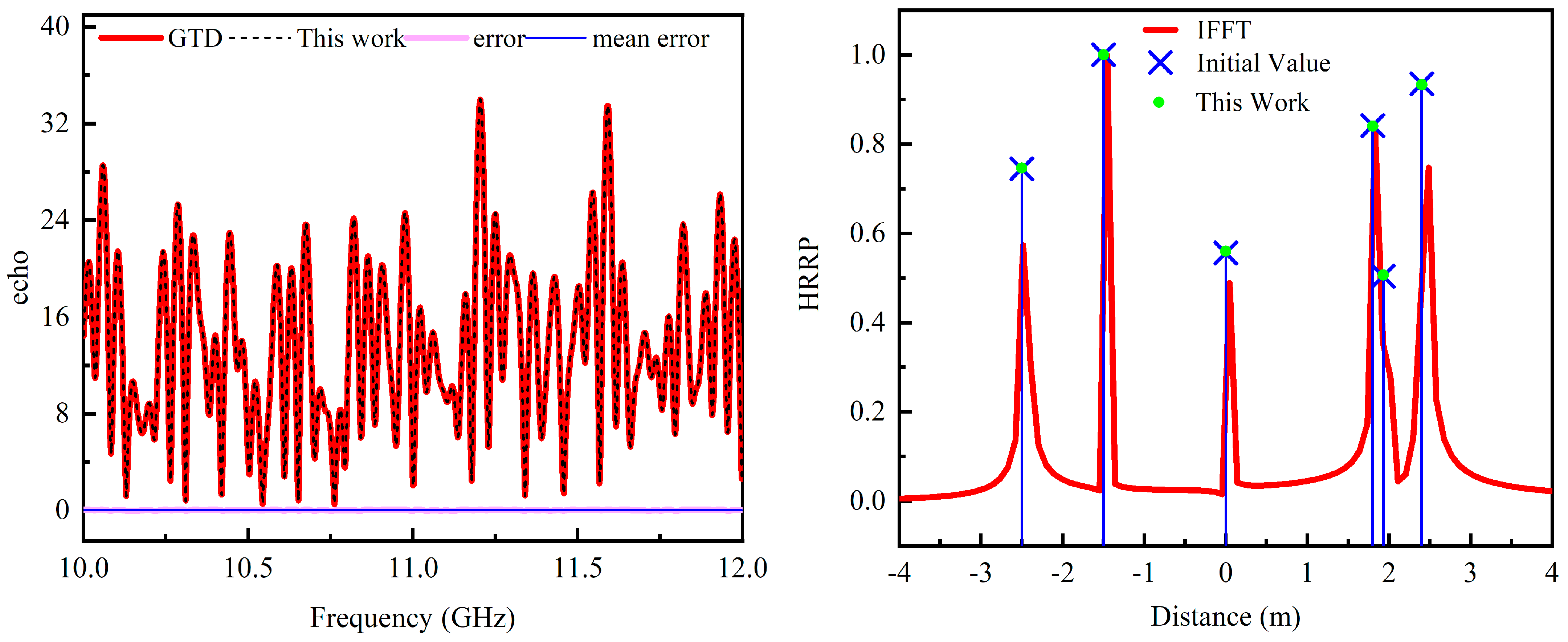
A simulation example is presented in this section to verify the effectiveness of the parameter extraction algorithm. The radar echo is generated by substituting the SCs information (as shown in Group A, Table 2), including amplitude, position, and type, into Equation (7). Subsequently, the adaptive TLS-ESPRIT algorithm is used to extract SC information (as shown in Group B) from the simulated radar echo. The starting frequency of the radar was set to 10 GHz with a frequency step of 1.6 MHz and a frequency point of 1000. The effectiveness of the adaptive TLS-ESPRIT algorithm is verified by comparing the preset SCs information (Group A) with the extracted information (Group B). Furthermore, the radar echo and HRRP results are displayed in Figure 3. It can be seen that the two sets of echo data are almost identical, with an average error of 0.04. In addition, the HRRP result is provided in Figure 3 in order to verify that the SCM can accurately represent the total scattered field from another perspective. The simulation results reveal the limitations of the IFFT method in effectively extracting SCs residing within the same resolution unit. Conversely, the adaptive TLS-ESPRIT method exhibits higher extraction accuracy when dealing with dense SCs, offering a significant advantage over traditional methods.
Table 2.
Extracted SC information.
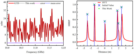
Figure 3.
Validation of the effectiveness of the adaptive TLS-ESPRIT algorithm.
3. RCS Intelligent Extrapolation Technology Guided by Physical Mechanisms
3.1. The Challenges Faced by SCM in Application
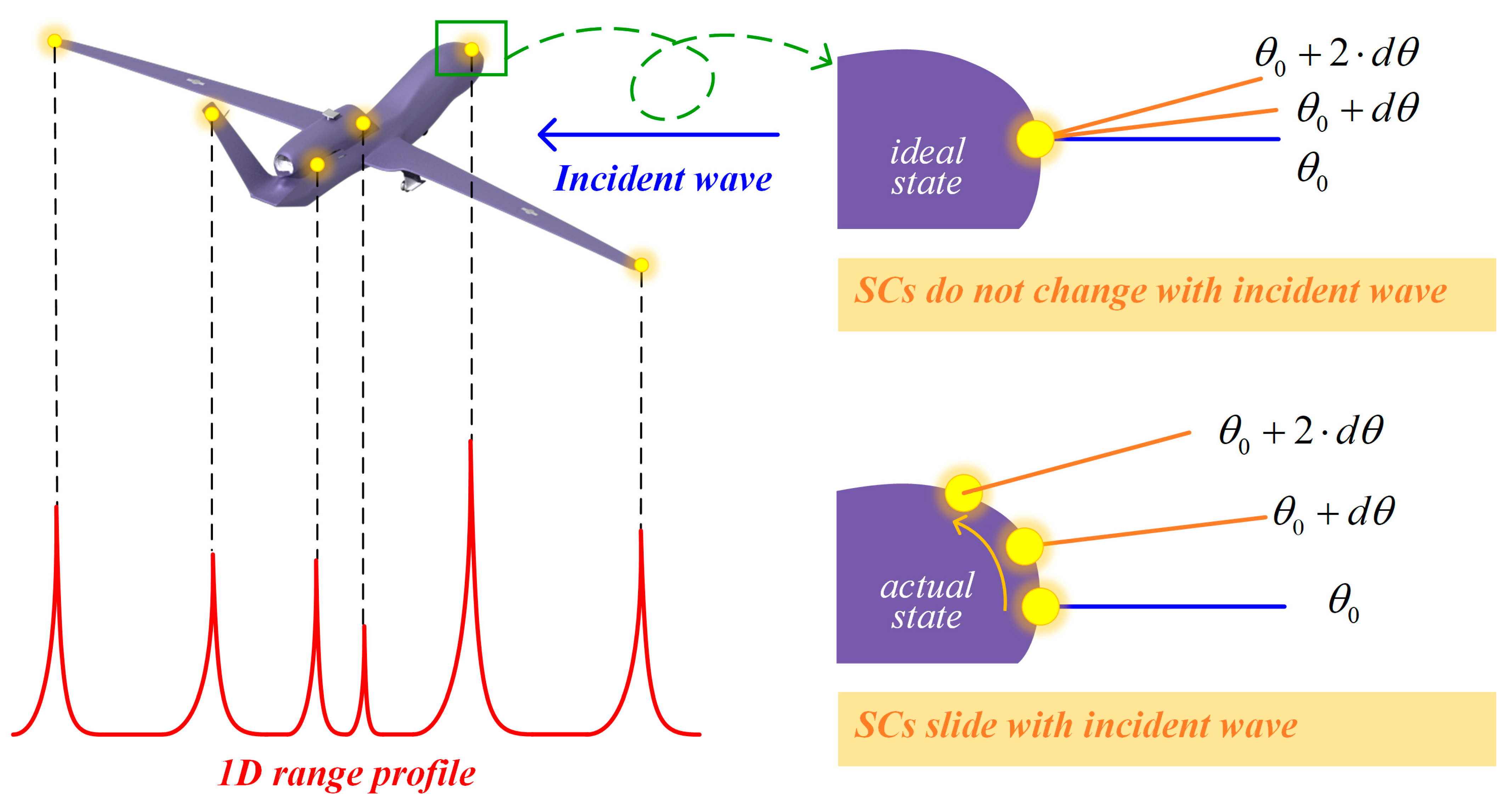
In Section 2, the scattered echoes of the target are succinctly represented by the SCM. However, practical RCS extrapolation using SCM encounters challenges, as illustrated in Figure 4. A direct relationship exists between the scattering echo of a target and the corresponding SCM when illuminated by an incident wave. At this point, the 1D ranging profile can be acquired, which reflects the position and amplitude of the SCs in the radar line-of-sight direction. Ideally, the SCs of the target exhibit invariance with respect to both the operating frequency and incident angle of the illuminating wave. Our goal of RCS extrapolation can be readily achieved if this assumption holds: construct the SCM of the target from easily accessible LFB echoes and generate the RCS in the HFB directly based on the established SCM and GTD theory. However, in reality, the position of the SCs will change when the angle (the case shown in Figure 4) or the operating frequency is changed, especially in smooth regions such as the nose and engine of an aircraft. Consequently, the position of the SCs may exhibit a slight slide on the target surface with variations in frequency or angle. This phenomenon renders the SCM constructed from the LFB data unsuitable as a direct substitute for the SCM in the HFB. Even minor discrepancies between the two models can introduce non-negligible errors in HFB RCS extrapolation using this approach.
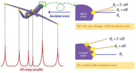
Figure 4.
Positional shift of scattering center with incident angle.
3.2. Artificial Neural Networks Incorporating Physical Mechanism
Considering that the SCs will slide on the target surface as the incident wave conditions change. Analytically determining the “slide value” by geometry relationships or radar parameters is challenging. This section will focus on strategies to address the challenges encountered. As shown in Figure 4, for the SC, we define the sliding value as , caused by the change in incident wave angle. The parameter sets of the SCs before and after this change are defined as and , respectively, and the correlation of SC parameters can be expressed as (20).
Similarly, a slight slide of SCs on the target surface will happen with a decrease in radar wavelength in the frequency domain of RCS extrapolation.
In (21), the corner labels HFB and LFB stand for the high-frequency bands and low-frequency bands, respectively, and represents the extrapolated band. It should be noted that in the complete radar sight, is a definite value, while is a random value, and is much smaller than . Based on this analysis, an intelligent RCS extrapolation technology that incorporates trend prediction and intelligent optimization is proposed in this paper, where is used as an approximate for in trend prediction, which is clearly feasible due to the minor differences between them. To account for the error introduced by this approximation, denoted as , an ANN is introduced in the intelligent optimization process. The specific technical route is outlined as follows.
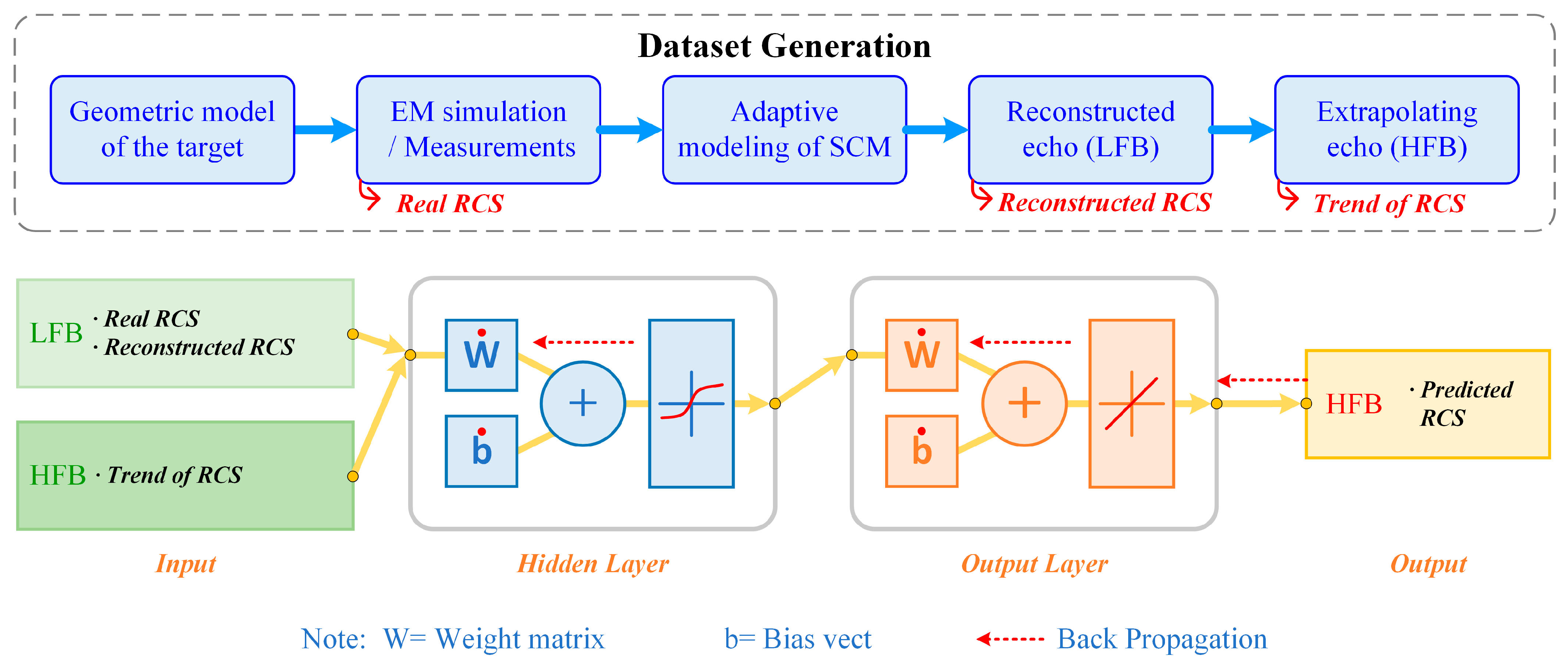
- Dataset Generation
To effectively train the neural network component of the SCM−ANN, we need to define the sample form and generate a comprehensive dataset. The supervised learning approach is chosen for this task because it allows us to leverage known relationships between inputs and outputs. In supervised learning tasks, samples consist of input features and corresponding outputs. The neural network gradually adjusts its parameters to improve prediction accuracy by learning multiple samples from the dataset. In this work, to incorporate the physical mechanism into the ANN, the input features of each sample are expanded to include the ordinal number, frequency, real RCS (obtained from SBR-PO/PTD or measurements), and reconstructed RCS (calculated using the LFB SCM), all within LFB. The corresponding output features consist of the frequency and extrapolated RCS within HFB. These RCS data can be obtained by (22)–(24).
According to the GTD, the radar echoes in the LFB can be reconstructed using the target’s SCM obtained from Section 2.2.
where represents the reconstructed echo by using SCM in the LFB. Furthermore, the SCM constructed from the LFB echoes is transplanted to the HFB, thus enabling the trend prediction of the scattered echoes in the HFB.
where is the trend of the target’s echo predicted by SCM, is the number of frequency points in HFB. The RCS of the target in the frequency domain can be acquired based on the scattered echoes by (23).
where is scattered echoes. Taking an echo obtained by SBR, , and into (24), the real RCS of the target, the reconstructed RCS in LFB, and the trend of RCS in HFB can be obtained, respectively.
These data will be used as samples for training networks. The construction of the dataset relies on intensive sampling from targets, frequencies, and angles. Table 3 illustrates an example of generating datasets, which will be used for numerical simulations and algorithm validation in Section 4. The dataset consists of HH-polarized RCS data with an angular interval of 0.5° along and .
Table 3.
Database construction.
- B.
- Bayesian Regularization ANN
The LFB dataset is constructed as described in A in the Section 3.2. In this section, machine learning technology that minimizes the loss function is used to build a training network for extrapolating the RCS in HFB.
Among the various types of machine learning algorithms, Bayesian regularization ANN was selected in this paper for its strong generalization capabilities and suitability for parallel computation. Specifically, a two-layer feedforward network with sigmoid hidden neurons and linear output neurons is constructed, as shown in Figure 5. Its structure ensures that the network can effectively address the multidimensional mapping problem with a sufficient number of samples and hidden layer neurons. Meanwhile, the adopted Bayesian regularization ANN utilizes the Levenberg–Marquardt algorithm to perform error backpropagation between the network output and the actual labels (Figure 5, red dashed line). The feedforward network facilitates the forward propagation of information, and the backpropagation algorithm adjusts the weights and biases collectively, enabling the training and learning of the neural network. The steps involved in constructing a Bayesian regularization ANN that incorporates physical mechanisms are as follows:

Figure 5.
The structure of neural networks.
Step 1: Initial settings. In this step, the initial settings of the network are determined in order to manage the intelligent optimization process. In this work, the number of iterations is set to 1000, and the number of neurons is 20. The mean square error (MSE) is used as the loss function, whose calculation formula is shown in (25).
where is the actual value and represents the predicted value.
Step 2: Import training data. In this step, a dataset consisting of a certain number of samples is used to train the Bayesian regularization ANN. This dataset includes real echoes, reconstructed echoes, and corresponding frequencies, etc. The purpose of this step is to establish a nonlinear mapping between the real RCS and the reconstructed RCS of the target in LFB.
Step 3: Train the network. The imported data are randomly decomposed into training, validation, and testing sets, comprising 70%, 15%, and 15% of the total data, respectively. These proportions are commonly used as defaults in ANN applications as a standard practice. Adjusting the number of neurons allows for a balance between the computational resource consumption and the nonlinear representation capability of the ANN when the ideal network is not acquired.
Step 4: RCS intelligent extrapolation. By utilizing the fully trained Bayesian regularization ANN network to predict the trend of RCS in HFB, the network will intelligently extrapolate the RCS values for HFB, relying on the established nonlinear relationships.
- C.
- Network Optimization
Network optimization is carried out throughout the construction of the dataset and the tuning of the training parameters to ensure sufficient prediction accuracy. Trend prediction data, incorporating physical mechanisms, are integrated into the training samples. This enables the ANN to obtain suitable initial solutions quickly. Optimizing the predictive power of ANN can be achieved by iterating through the network training process (steps 1 to 4). Potential actions during this strategy include retraining the network, increasing the number of hidden neurons, or expanding the training dataset. Nevertheless, ANN still must confront the issue of overfitting.
In this paper, Bayesian regularization [35] is used for network training due to its effectiveness in improving generalization, even in scenarios with limited data and high noise levels. The Bayesian framework offers a robust approach to preventing overfitting by incorporating prior distributions on the network weights. The first layer within this framework is as follows:
and the second layer of the Bayesian framework is as follows:
in which is a vector that contains all the ownership and bias values in the network; denotes the training dataset; and represent the parameters related to the density function; and represents the selected network structure.
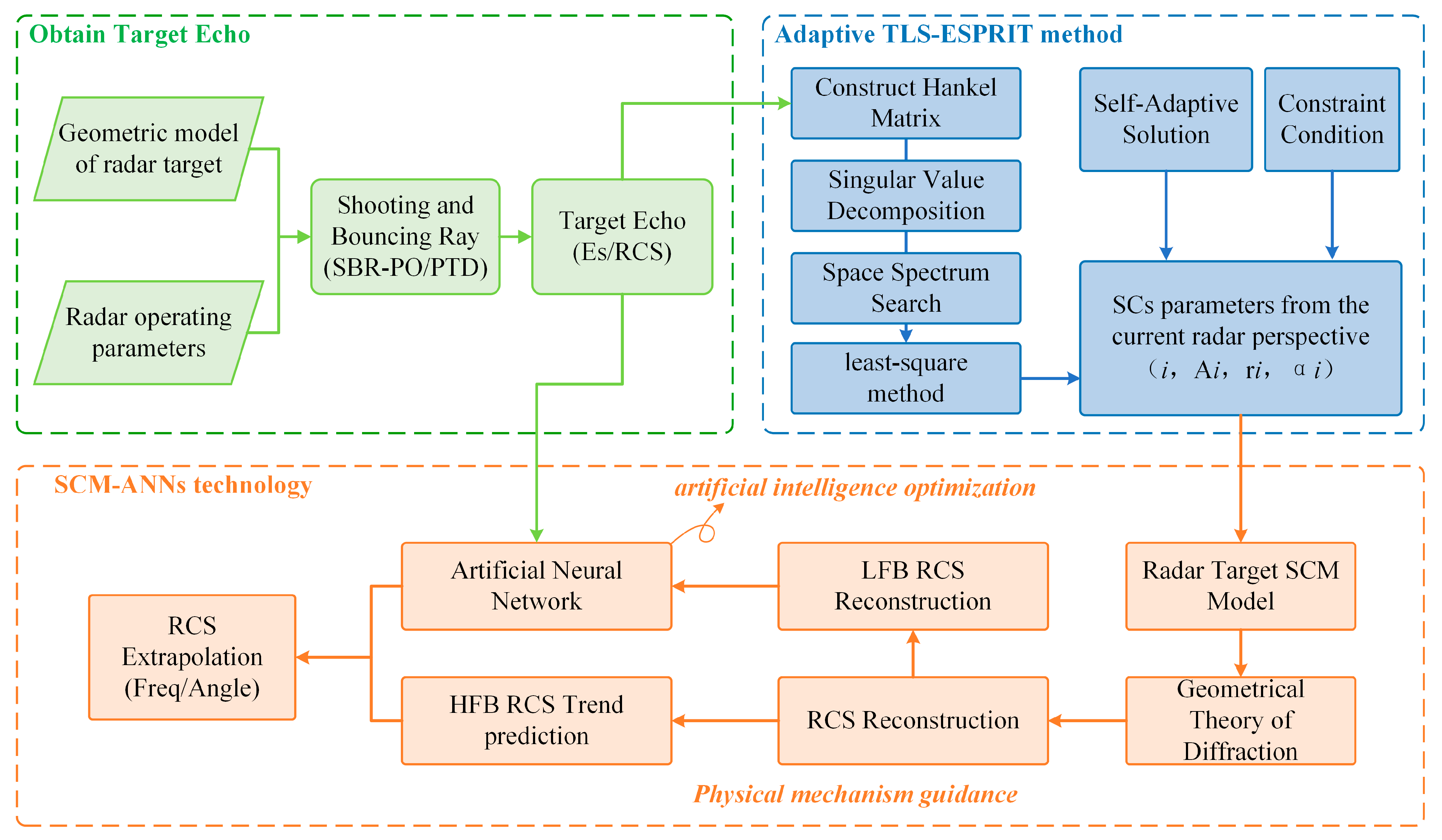
Implemented neural networks are optimized by combining physical mechanisms with Bayesian regularization, effectively resolving the overfitting problem encountered during training. The detailed technical framework of the SCM−ANN technology is illustrated in Figure 6, which is expanded from Figure 1.

Figure 6.
Technical route of SCM−ANN technology.
4. Numerical Simulation and Actual Measurement Verification
Numerical simulation and experimental measurement results are used to validate the effectiveness of the proposed SCM−ANN technology for RCS extrapolation in this section. The simulation examples encompass a variety of targets, angles of incidence, and radar operating bands.
4.1. Electromagnetic Simulation Verification
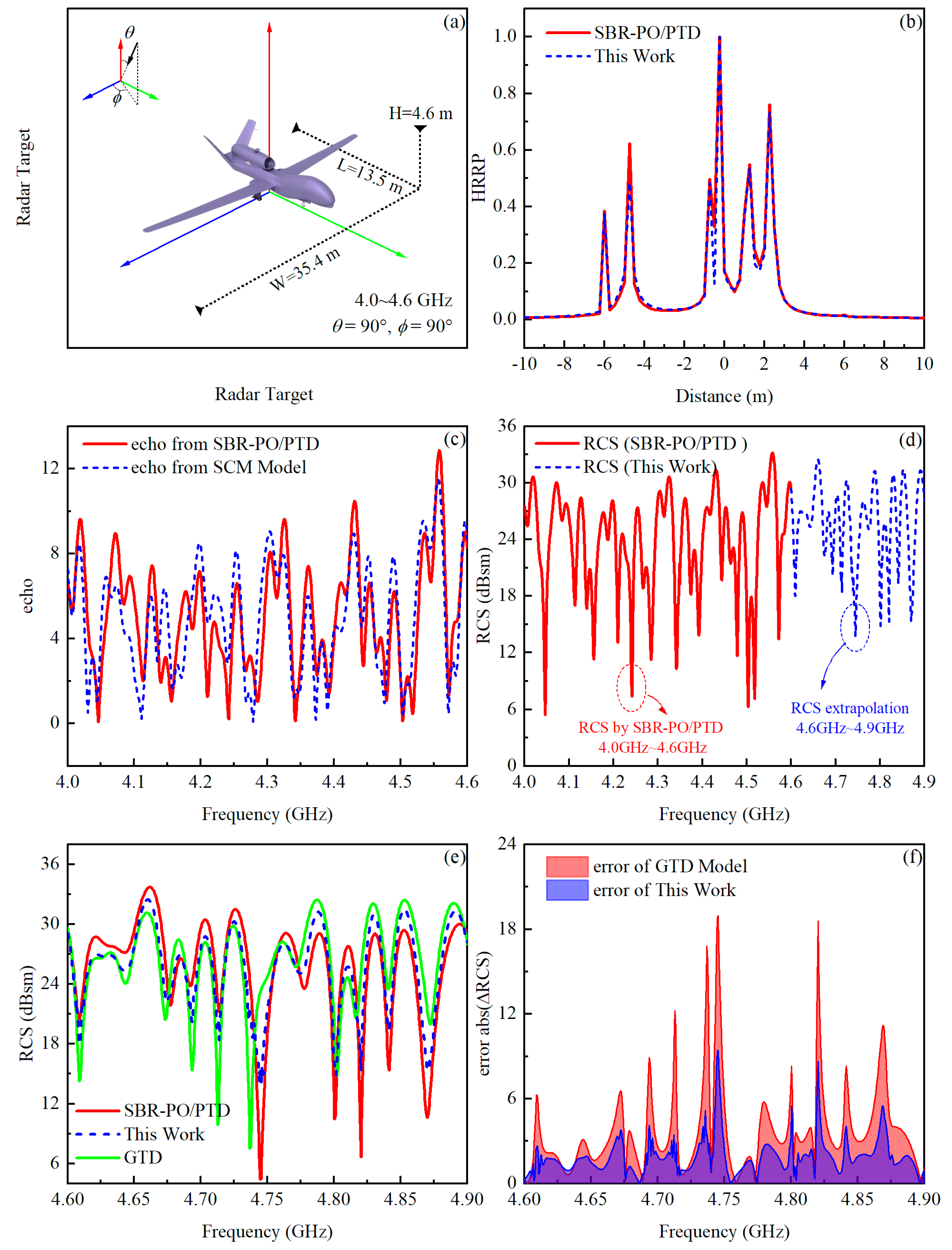
In the following, an aircraft model (13.5 m × 35.4 m × 4.6 m) is used to evaluate the effectiveness of the proposed method. The target material is PEC, which consists of 351,778 triangular patches. Figure 7, Figure 8, Figure 9 and Figure 10 display the simulation results, including the radar echoes from the SBR, the RCS extrapolation results obtained from the proposed SCM-ANN technology, and absolute errors, in which the absolute error is defined as follows:
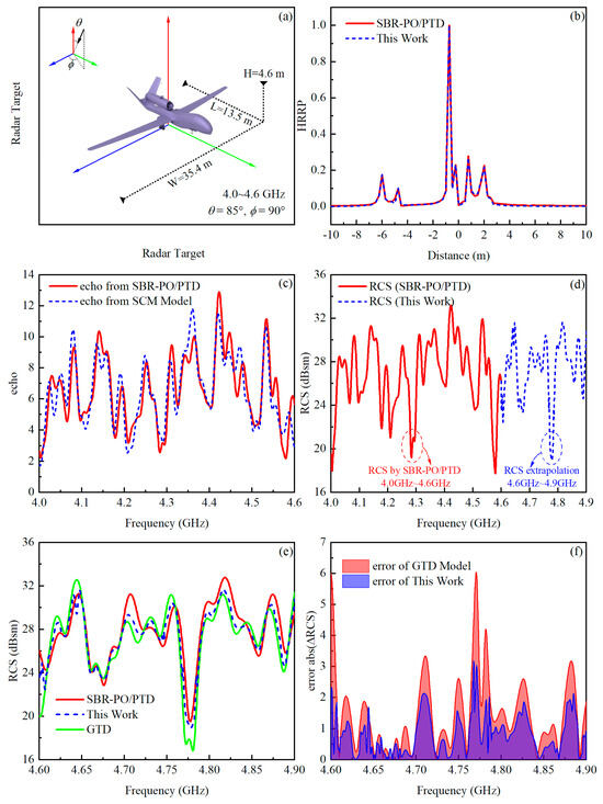
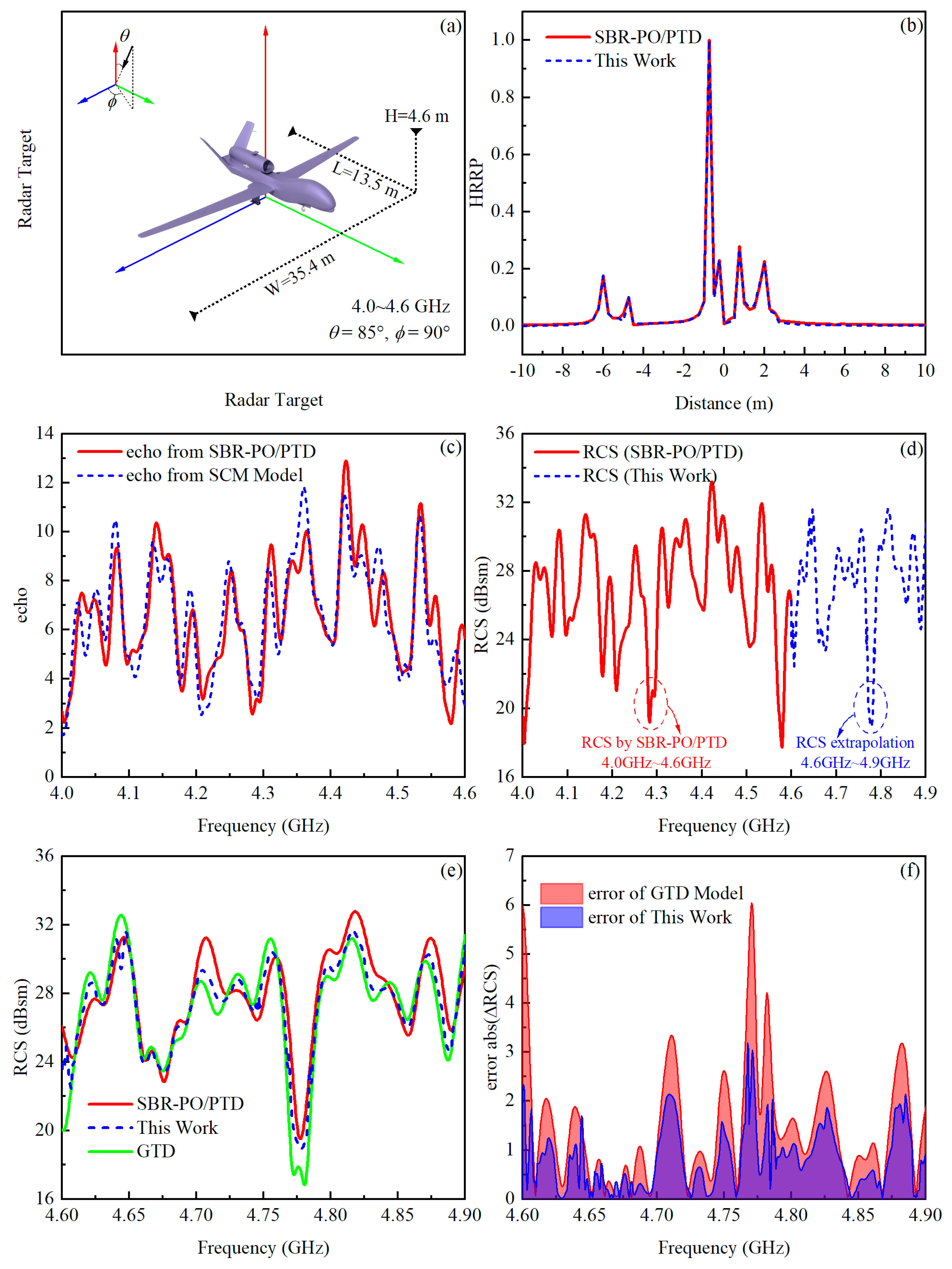
Figure 7.
Numerical simulation results of the SCM−ANN technology. (a) Geometry of the target; (b) comparison of the target’s HRRP; (c) comparison of radar echo in the LFB; (d) RCS extrapolation results; (e) comparison of RCS extrapolation results in the HFB; (f) comparison of errors of RCS extrapolation.
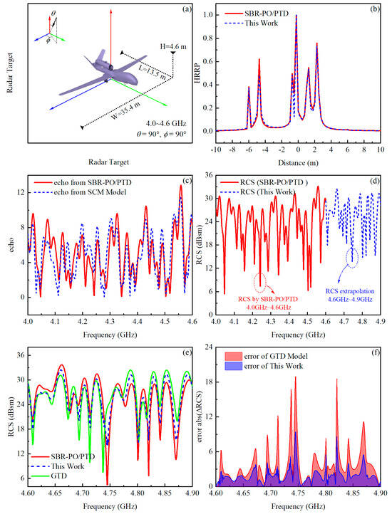
Figure 8.
Numerical simulation results of the SCM−ANN technology. (a) Geometry of the target; (b) comparison of the target’s HRRP; (c) comparison of radar echo in the LFB; (d) RCS extrapolation results; (e) comparison of RCS extrapolation results in the HFB; (f) comparison of errors of RCS extrapolation.
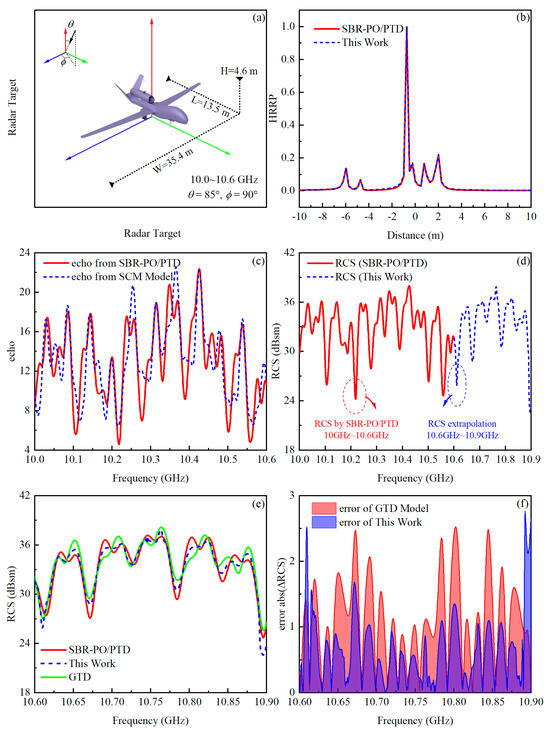
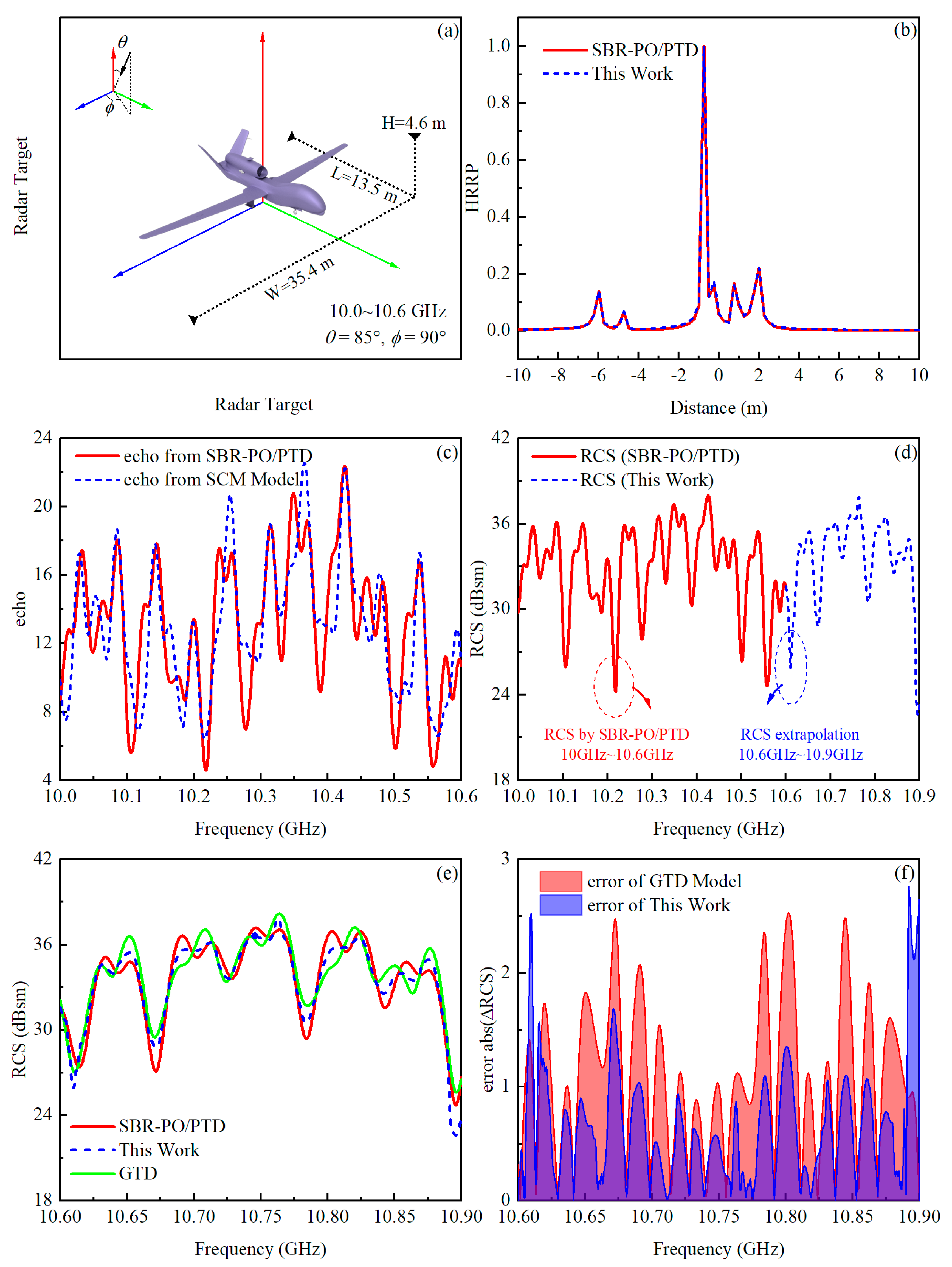
Figure 9.
Numerical simulation results of the SCM−ANN technology. (a) Geometry of the target; (b) comparison of the target’s HRRP; (c) comparison of radar echo in the LFB; (d) RCS extrapolation results; (e) comparison of RCS extrapolation results in the HFB; (f) comparison of errors of RCS extrapolation.
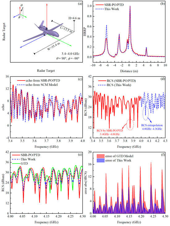
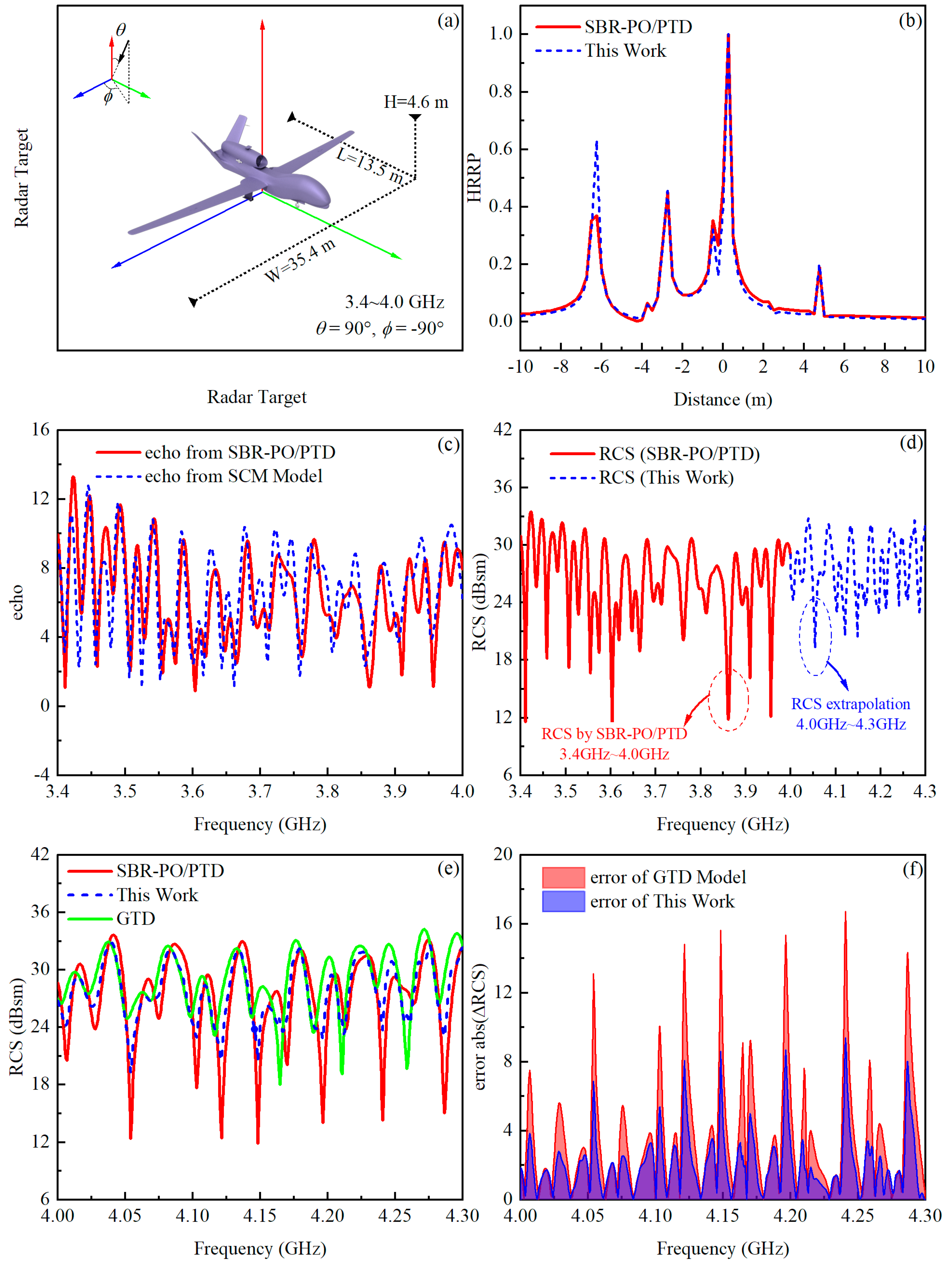
Figure 10.
Numerical simulation results of the SCM−ANN technology. (a) Geometry of the target; (b) comparison of the target’s HRRP; (c) comparison of radar echo in the LFB; (d) RCS extrapolation results; (e) comparison of RCS extrapolation results in the HFB; (f) comparison of errors of RCS extrapolation.
In Figure 7, Figure 8, Figure 9 and Figure 10, subfigure (a) illustrates the target geometry and incident wave parameters, and subfigure (b) presents the HRRP results derived from both the radar and reconstructed echoes. Subfigure (c) compares the radar echoes obtained by the aforementioned two methods. Subfigures (b) and (c) provide different perspectives to verify the GTD model’s ability to accurately represent the scattered field. Subfigure (d) in Figure 7, Figure 8, Figure 9 and Figure 10 demonstrates the RCS extrapolation results using the proposed SCM−ANN technology. The approach can successfully achieve a 50% frequency extrapolation range based on the LFB scattering characteristics. Subfigure (e) presents a comparison of the RCS results in the extrapolated frequency band. Subfigure (f) shows the error associated with both the GTD model alone and the proposed SCM−ANN technology. The results clearly demonstrate a significant reduction in RCS extrapolation error when employing the SCM−ANN approach.
Figure 7 shows the simulation results of RCS extrapolation for an incident wave frequency range of 4.0~4.6 GHz, an incidence angle of . The LFB scattering characteristics were obtained by the SBR-PO/PTD algorithm, which is considered the real radar echo in this simulation, and served as the foundation for extrapolating the RCS to a higher-frequency band of 4.6~4.9 GHz with the frequency increment of 0.6 MHz.
Figure 8 shows the simulation results of RCS extrapolation for an incidence angle of , and the other simulation parameters are consistent with Figure 7. At this time, the incident wave was shining on the head of the airplane. In subfigure (b) of the HRRP results, the amplitude characteristics of the strong scattering points are significantly different between Figure 7 and Figure 8.
Figure 9 shows the simulation results of RCS extrapolation with different frequency bands. The incident wave frequency is 10~10.6 GHz, and the incident angle is . The RCS extrapolation frequency band is 10.6~10.9 GHz with a frequency step of 0.6 MHz.
Figure 10 shows the simulation results of RCS extrapolation for an incident wave frequency range of 3.4~4.0 GHz, an incidence angle of . The incident wave is shining on the tail of the airplane. The extrapolation band of RCS is 4.0~4.3 GHz, with the frequency step being 0.6 MHz. Simulation results show that the proposed method can also execute RCS extrapolation at lower-frequency bands.
It should be noted that there exist a few frequency points exhibiting negative optimization cases in subfigure (e) of Figure 7, Figure 8, Figure 9 and Figure 10 (especially Figure 9). These instances arise due to the influence of extreme values or inflection points in the training samples, which can interfere with the prediction of the ANN and lead to increased error. Removing the impact of such extreme points will be treated as a follow-up.
The simulation specifics for the four examples are elaborated in Table 4. The “echo of GTD” signifies the average error between the reconstructed echo and the real echo, while the “echo of SCM−ANN” denotes the average error between the echo obtained through SCM−ANN technology and the real echo. The results demonstrate that the intelligent extrapolation technology, SCM−ANN, inspired by the physical mechanism, achieves a remarkable reduction in error exceeding 40% for RCS extrapolation. These simulation results verify the effectiveness of the proposed method.
Table 4.
Numerical simulation results.
4.2. Field Testing and Verification
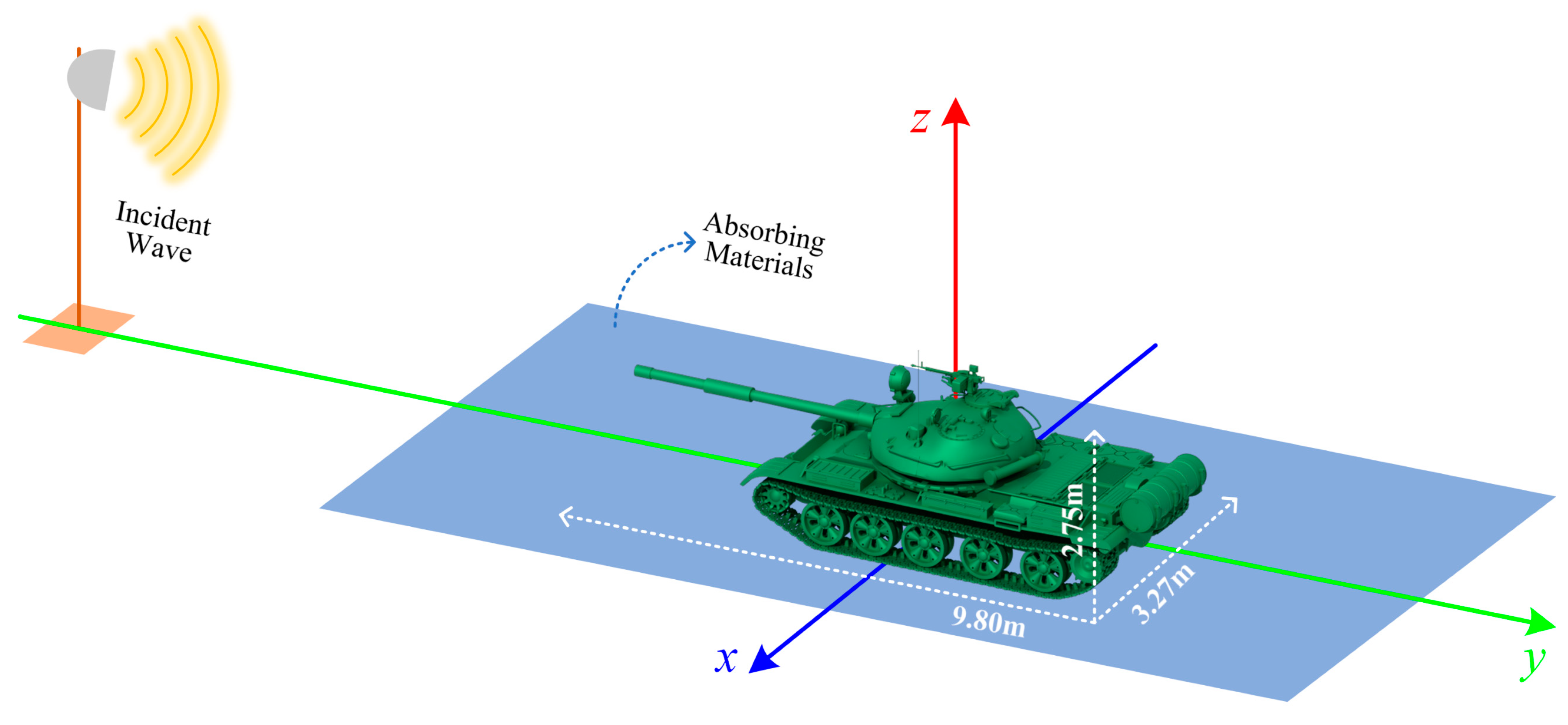
In this section, measurement data from real tank targets are employed to validate the feasibility of the proposed method. The schematic diagram of the measurement system is shown in Figure 11. Absorbing materials are densely placed around the target to ensure the acquisition of scattered echoes with minimal background radiation. In this example, the polar angle is 30 degrees, and the azimuth angle is 270 degrees. The LFB is set as 1.0~1.666 GHz.
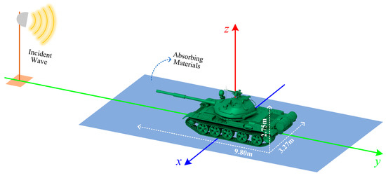
Figure 11.
Schematic of low radiation background measurement system.
Figure 12a,b show the HRRP and echo results obtained from the measured data and reconstructed echoes, respectively. These subfigures further confirm that the GTD model can represent the scattered field well in the LFB. Figure 12c,d present the RCS extrapolation results and the corresponding error distribution of the GTD model and the proposed SCM−ANN. Notably, as depicted in Figure 12d, the application of SCM−ANN leads to a reduction in the average error from 5.4 dB to 3.7 dB, and the proposed method successfully achieves a notable reduction in extrapolation error.
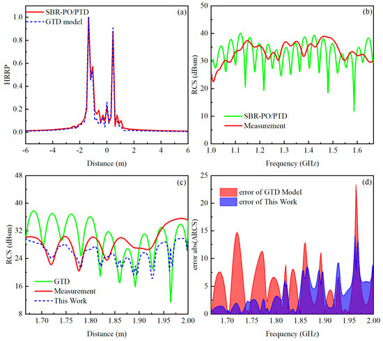
Figure 12.
Measurement results of SCM−ANN technology. (a) Comparison of the target’s HRRP; (b) comparison of RCS in LFB; (c) RCS extrapolation results; (d) error of RCS extrapolation.
5. Discussion
In this paper, an RCS extrapolation technology named SCM−ANN, which incorporates physical mechanisms and neural networks, is proposed and validated to achieve accurate HFB RCS prediction using limited LFB data. The proposed method demonstrates significant performance improvements, achieving 50% bandwidth RCS extrapolation and 40% error reduction compared to traditional methods. Furthermore, benefiting from the SC adaptive modeling capability, the SCM−ANN technology is particularly suitable for non-cooperative targets. These findings showcase the potential of SCM−ANN for reliable RCS prediction across a wide frequency range. Further analysis of the results reveals the following limitations of the SCM−ANN technology:
(a) Negative optimization was observed at certain frequency points, particularly in Figure 9e. These instances arise due to the influence of extreme values or inflection points in the training samples, which can interfere with the prediction of the ANN’s prediction and lead to increased error;
(b) Compared to the numerical simulation, the error reduction rate (from 40% to 35%) and the number of negative optimization points in the field test deteriorate slightly. This is primarily attributed to the inherent spurious interference in the measurement system. Obviously, background noise and system errors deviate from the idealized assumptions of the GTD model, introducing disturbances during the SCM construction process.
Addressing the performance limitations highlighted above will be a priority in our subsequent research. Further investigation and improvements are needed to mitigate the effects of negative optimization and spurious interference in real-world applications.
6. Conclusions
An SCM−ANN technology is proposed in this paper for intelligent RCS extrapolation of non-cooperative radar targets. By incorporating physical mechanisms driven by SCM as a priori information, the proposed method achieves enhanced efficiency and accuracy in RCS extrapolation. Compared to numerical prediction methods that are highly dependent on captured data, the proposed method utilizes GTD to provide physically guided trend prediction, enabling its application to more complex radar targets and wider frequency extrapolation ranges. In addition, the introduction of a neural optimization network in the proposed method results in a remarkable error reduction of over 35% compared to the traditional SCM-based RCS extrapolation method. Simulation and measured examples with various targets, frequency bands, and incidence angles validate the effectiveness of the proposed method. The proposed SCM−ANN provides a feasible technology solution for extrapolating the HFB RCS information of a target. Its potential application extends to various domains, including the characterization of scattering behavior in non-measurable frequency bands, the rapidly constructing target database for radar system design and analysis, and the development of advanced target recognition and classification techniques.
Author Contributions
Writing—original draft preparation, F.-Y.Z. and S.-R.C.; methodology, F.-Y.Z. and L.-X.G.; investigation, Z.-X.H. and S.-R.C.; validation, Y.-F.Z., F.-Y.Z. and L.-X.G. All authors have read and agreed to the published version of the manuscript.
Funding
This work was supported in part by the National Natural Science Foundation of China (grant nos. 62231021, U21A20457, 62201435), in part by the Natural Science Basic Research Program of Shaanxi (grant no. 2023-JC-YB-537), in part by the Fundamental Research Funds for the Central Universities (grant nos. QTZX23010, ZYTS23068, YJSJ24005), and in part by the Aeronautical Science Foundation of China (grant no. 20172081009).
Data Availability Statement
The raw data supporting the conclusions of this article will be made available by the authors on request.
Conflicts of Interest
The authors declare no conflicts of interest.
References
- Martorella, M.; Giusti, E.; Demi, L.; Zhou, Z.; Cacciamano, A.; Berizzi, F.; Bates, B. Target Recognition by Means of Polarimetric ISAR Images. Trans. Aerosp. Electron. Syst. 2011, 47, 225–239. [Google Scholar] [CrossRef]
- Novak, L.M.; Halversen, S.D.; Owirka, G.; Hiett, M. Effects of polarization and resolution on SAR ATR. Trans. Aerosp. Electron. Syst. 1997, 33, 102–116. [Google Scholar] [CrossRef]
- Wang, H.; Wei, B.; Liu, H. A Fast Method for SBR-Based Multiaspect Radar Cross Section Simulation of Electrically Large Targets. IEEE Antennas Wirel. Propag. Lett. 2022, 21, 1920–1924. [Google Scholar] [CrossRef]
- Fan, T.Q.; Guo, L.X.; Liu, W. A Novel OpenGL-Based MoM/SBR Hybrid Method for Radiation Pattern Analysis of an Antenna Above an Electrically Large Complicated Platform. IEEE Trans. Antennas Propag. 2016, 64, 201–209. [Google Scholar] [CrossRef]
- He, W.J.; Liu, X.D.; Wu, B.Y.; Yang, M.L.; Sheng, X.Q. High-Performance Simulation of Electromagnetic Scattering by 3D Objects Using the GPU-accelerated Parallel MLFMA. In Proceedings of the 2023 International Applied Computational Electromagnetics Society Symposium (ACES-China), Hangzhou, China, 16–18 August 2023; pp. 1–2. [Google Scholar]
- Ling, H.; Chou, R.C.; Lee, S.W. Shooting and bouncing rays: Calculating the RCS of an arbitrarily shaped cavity. IEEE Trans. Antennas Propag. 1989, 37, 194–205. [Google Scholar] [CrossRef]
- Shah, M.A.; Tokgöz, Ç.; Salau, B.A. Radar Cross Section Prediction Using Iterative Physical Optics with Physical Theory of Diffraction. IEEE Trans. Antennas Propag. 2022, 70, 4683–4690. [Google Scholar] [CrossRef]
- Kasdorf, S.; Troksa, B.; Key, C.; Harmon, J.; Notaroš, B.M. Advancing Accuracy of Shooting and Bouncing Rays Method for Ray-Tracing Propagation Modeling Based on Novel Approaches to Ray Cone Angle Calculation. IEEE Trans. Antennas Propag. 2021, 69, 4808–4815. [Google Scholar] [CrossRef]
- Aguilar, A.G.; Van Tonder, J.; Jakobus, U.; Illenseer, F. Overview of recent advances in the electromagnetic field solver FEKO. In Proceedings of the 2015 9th European Conference on Antennas and Propagation (EuCAP), Lisbon, Portugal, 13–17 April 2015; pp. 1–5. [Google Scholar]
- Tao, Y.B.; Lin, H.; Bao, H. KD-tree based fast ray tracing for RCS prediction. Prog. Electromagn. Res. 2008, 81, 329–341. [Google Scholar] [CrossRef]
- Mansukhani, J.; Penchalaiah, D.; Bhattacharyya, A. Rcs based target classification using deep learning methods. In Proceedings of the 2021 2nd International Conference on Range Technology (ICORT), Balasore, India, 5–6 August 2021; pp. 1–5. [Google Scholar]
- Zhao, J.C.; Zhang, K.; Yang, Z.; Li, Y. Research on Radar Cross Section Scaling Relation based on Neural Network. In Proceedings of the 2022 IEEE Conference on Antenna Measurements and Applications (CAMA), Guangzhou, China, 14–17 December 2022; pp. 1–4. [Google Scholar]
- Chen, H.; Yang, C.; Du, Y. Machine learning-assisted analysis of polarimetric scattering from cylindrical components of vegetation. IEEE Trans. Geosci. Remote Sens. 2018, 57, 155–165. [Google Scholar] [CrossRef]
- Xiao, D.H.; Guo, L.X.; Liu, W.; Hou, M.Y. Efficient RCS prediction of the conducting target based on physics-inspired machine learning and experimental design. IEEE Antennas Wirel. Propag. Lett. 2020, 69, 2274–2289. [Google Scholar] [CrossRef]
- Jacobs, J.P.; Du Plessis, W. Efficient modeling of missile RCS magnitude responses by Gaussian processes. IEEE Antennas Wirel. Propag. Lett. 2017, 16, 3228–3231. [Google Scholar] [CrossRef]
- Lee, S.Y.; Park, C.S.; Park, K.; Lee, H.J.; Lee, S. A Physics-informed and data-driven deep learning approach for wave propagation and its scattering characteristics. Eng. Comput.-Ger. 2023, 39, 2609–2625. [Google Scholar] [CrossRef]
- Wei, Z.; Chen, X.D. Deep-learning schemes for full-wave nonlinear inverse scattering problems. IEEE Trans. Geosci. Remote Sens. 2018, 57, 1849–1860. [Google Scholar] [CrossRef]
- Liu, J.; He, S.Y.; Zhang, L.; Zhang, Y.H.; Zhu, G.Q.; Yin, H.C.; Yan, H. An Automatic and Forward Method to Establish 3-D Parametric Scattering Center Models of Complex Targets for Target Recognition. IEEE Trans. Geosci. Remote Sens. 2020, 58, 8701–8716. [Google Scholar] [CrossRef]
- He, S.Y.; Hua, M.B.; Zhang, Y.H.; Du, X.Y.; Zhang, F. Forward Modeling of Scattering Centers From Coated Target on Rough Ground for Remote Sensing Target Recognition Applications. IEEE T. Geosci. Remote. 2024, 62, 1–17. [Google Scholar] [CrossRef]
- Cui, S.; Li, S.; Yan, H. A method of 3-D scattering center extraction based on ISAR images. In Proceedings of the 2016 IEEE International Conference on Electronic Information and Communication Technology (ICEICT), Harbin, China, 20–22 August 2016; pp. 439–442. [Google Scholar]
- Qu, Q.Y.; Guo, K.Y.; Sheng, X.Q. Scattering Centers Induced by Creeping Waves on Cone-Shaped Targets in Bistatic Mode. IEEE T. Antenn. Propag. 2015, 63, 3257–3262. [Google Scholar] [CrossRef]
- Huang, K.; He, S.Y.; Zhang, Y.H.; Yin, H.C.; Bian, Z.D.; Zhu, G.Q. Composite Scattering Analysis of the Ship on a Rough Surface Based on the Forward Parametric Scattering Center Modeling Method. IEEE Antennas Wirel. Propag. Lett. 2019, 18, 2493–2497. [Google Scholar] [CrossRef]
- Wang, J.; Zhou, J.J. Modified MEMP method for 2D scattering center measurement based on GTD model. In Proceedings of the 2008 International Conference on Microwave and Millimeter Wave Technology (ICMMT), Nanjing, China, 21–24 April 2008; pp. 987–990. [Google Scholar]
- Zheng, S.Y.; Zhang, X.K.; Guo, Y.D.; Zong, B.F.; Xu, J.H. An improved 2D-TLS-ESPRIT algorithm of GTD model parameter estimation. J. Beijing Univ. Aeronaut. Astronaut. 2020, 46, 1982–1989. [Google Scholar]
- Yun, D.J.; Jung, H.; Kang, H.; Kim, J.; Park, I.Y.; Lee, H.R.; Kim, Y.D. Scattering Center Extraction for ISAR Image using Deep Neural Network. In Proceedings of the 2023 20th European Radar Conference (EuRAD), Berlin, Germany, 20–22 September 2023; pp. 177–180. [Google Scholar]
- Wei, Y.; Li, J.; Gu, C. Study on two-dimensional electromagnetic scattering based on BP neural network. In Proceedings of the 2022 IEEE 4th International Conference on Civil Aviation Safety and Information Technology (ICCASIT), Dali, China, 12–14 October 2022; pp. 888–891. [Google Scholar]
- Fan, T.Q.; Guo, L.X.; Lv, B.; Liu, W. An Improved Backward SBR-PO/PTD Hybrid Method for the Backward Scattering Prediction of an Electrically Large Target. IEEE Antennas Wirel. Propag. Lett. 2016, 15, 512–515. [Google Scholar] [CrossRef]
- Ando, M.; Lu, P. Geometrical optics and diffraction extracted from Physical Optics by surface to line integral reduction using modified edge representation. In Proceedings of the Asia-Pacific Microwave Conference 2011, Melbourne, Australia, 5–8 December 2011; pp. 1937–1940. [Google Scholar]
- Jin, K.S.; Suh, T.I.; Suk, S.H.; Kim, B.C.; Kim, H.T. Fast Ray Tracing Using A Space-Division Algorithm for RCS Prediction. J. Electromagnet. Wave 2006, 20, 119–126. [Google Scholar] [CrossRef]
- Guo, W.; Yang, M.; Chen, B.; Zheng, G. Joint DOA and polarization estimation using MUSIC method in polarimetric MIMO radar. In Proceedings of the IET International Conference on Radar Systems (Radar 2012), Glasgow, UK, 22–25 October 2012; pp. 1–4. [Google Scholar]
- Ning, Y.M.; Ma, S.; Meng, F.Y.; Wu, Q. DOA Estimation Based on ESPRIT Algorithm Method for Frequency Scanning LWA. IEEE Commun. Lett. 2020, 24, 1441–1445. [Google Scholar] [CrossRef]
- Sahnoun, S.; Usevich, K.; Comon, P. Multidimensional ESPRIT for Damped and Undamped Signals: Algorithm, Computations, and Perturbation Analysis. IEEE Trans. Signal Process. 2017, 65, 5897–5910. [Google Scholar] [CrossRef]
- Zhu, F.Y.; Chai, S.R.; Zou, Y.F.; He, Z.X.; Guo, L.X. An Efficient and Accurate RCS Reconstruction Technique Using Adaptive TLS-ESPRIT Algorithm. IEEE Antennas Wirel. Propag. Lett. 2024, 23, 49–53. [Google Scholar] [CrossRef]
- Zheng, S.Y.; Zhang, X.K.; Zong, B.F.; Li, J. GTD Model Parameters Estimation Based on Improved LS-ESPRIT Algorithm. In Proceedings of the 2019 Photonics & Electromagnetics Research Symposium (PIERS), Xiamen, China, 17–20 December 2019; pp. 2282–2289. [Google Scholar]
- Fiorentini, N.; Pellegrini, D.; Losa, M. Overfitting prevention in accident prediction models: Bayesian regularization of artificial neural networks. Transp. Res. Rec. 2023, 2677, 1455–1470. [Google Scholar] [CrossRef]

Disclaimer/Publisher’s Note: The statements, opinions and data contained in all publications are solely those of the individual author(s) and contributor(s) and not of MDPI and/or the editor(s). MDPI and/or the editor(s) disclaim responsibility for any injury to people or property resulting from any ideas, methods, instructions or products referred to in the content. |
© 2024 by the authors. Licensee MDPI, Basel, Switzerland. This article is an open access article distributed under the terms and conditions of the Creative Commons Attribution (CC BY) license (https://creativecommons.org/licenses/by/4.0/).