
An Improved Underwater Visual SLAM through Image Enhancement and Sonar Fusion


Abstract
:1. Introduction
- Image-Level Enhancements: The proposed method integrates image brightness enhancement and suspended particulate removal techniques. This significantly increases the probability of the successful detection of visual feature points after application.
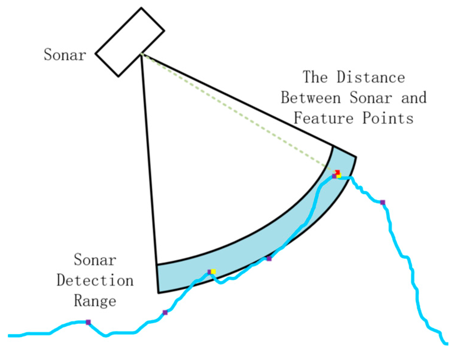
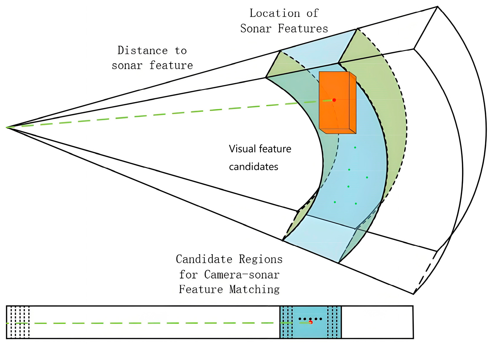
- Geometric Feature Association: From a spatial geometry perspective, a feature-association method that integrates sonar acoustic features with visual features is proposed, enabling visual features to obtain depth information.
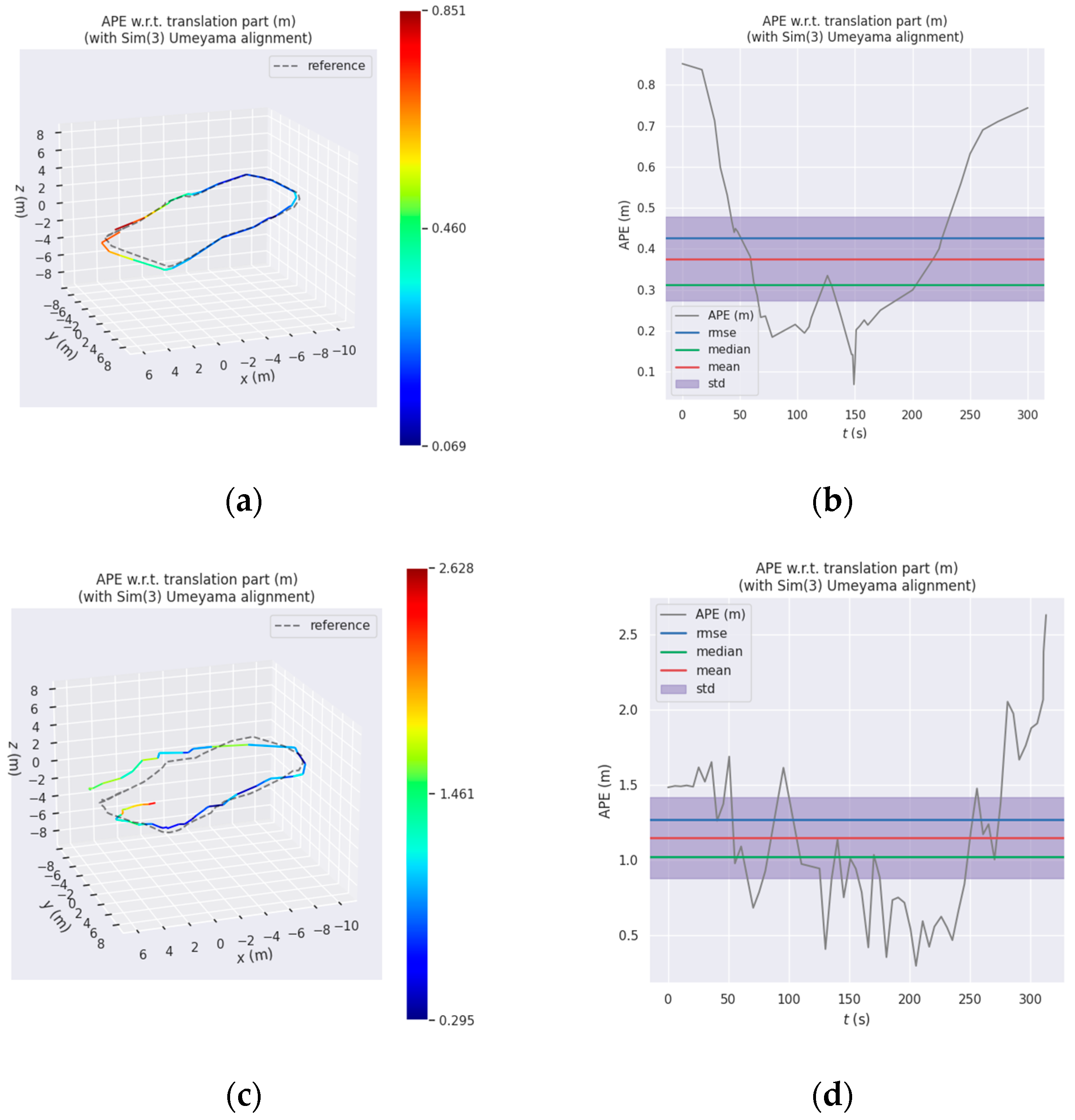
- Benchmarking with AFRL Dataset: A comparative analysis is conducted using the AFRL dataset against the classical OKVIS visual SLAM framework. This tests the limitations of traditional frameworks in underwater datasets and demonstrates the feasibility of the proposed method.
2. Related Work
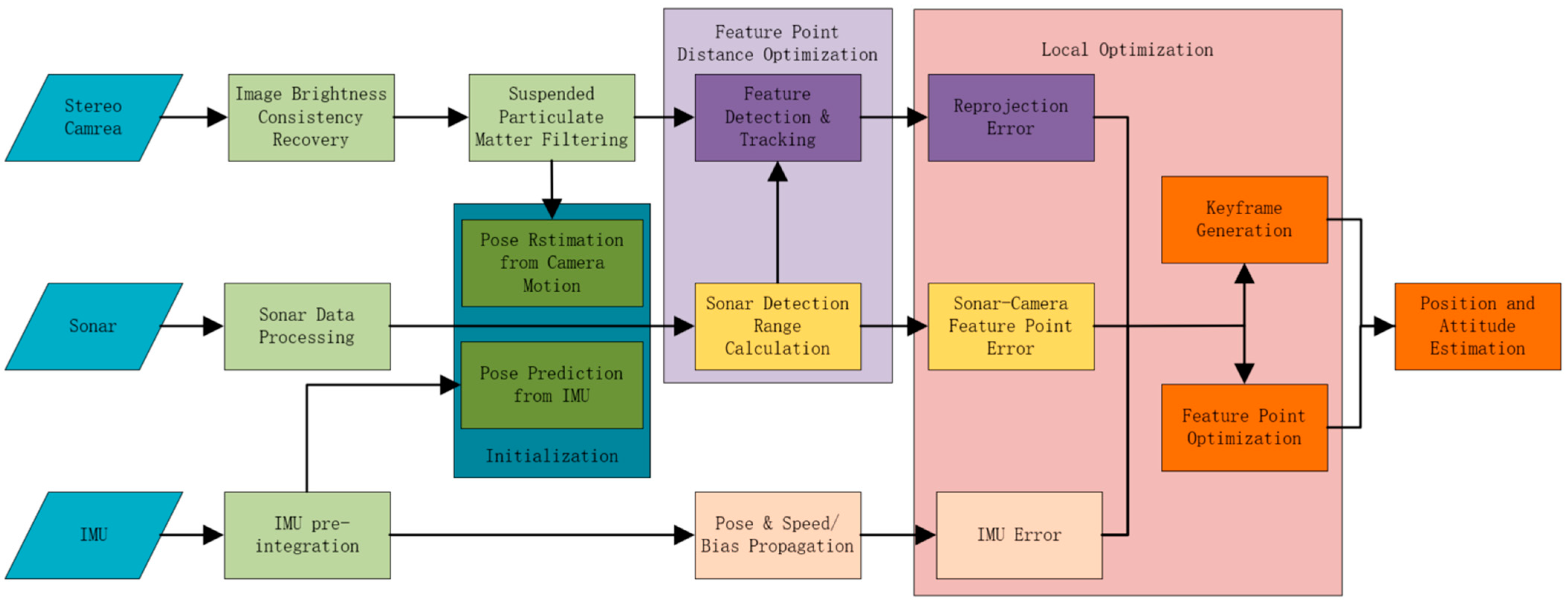
3. System Overview
4. Proposed Method
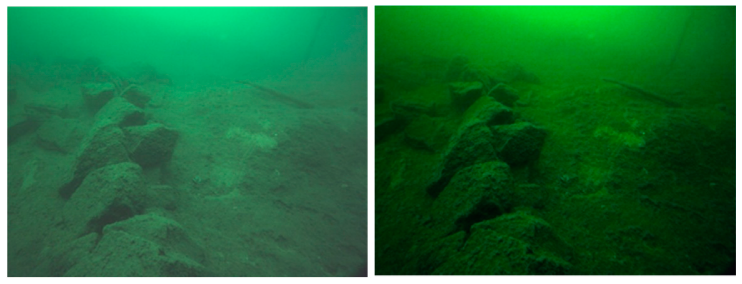
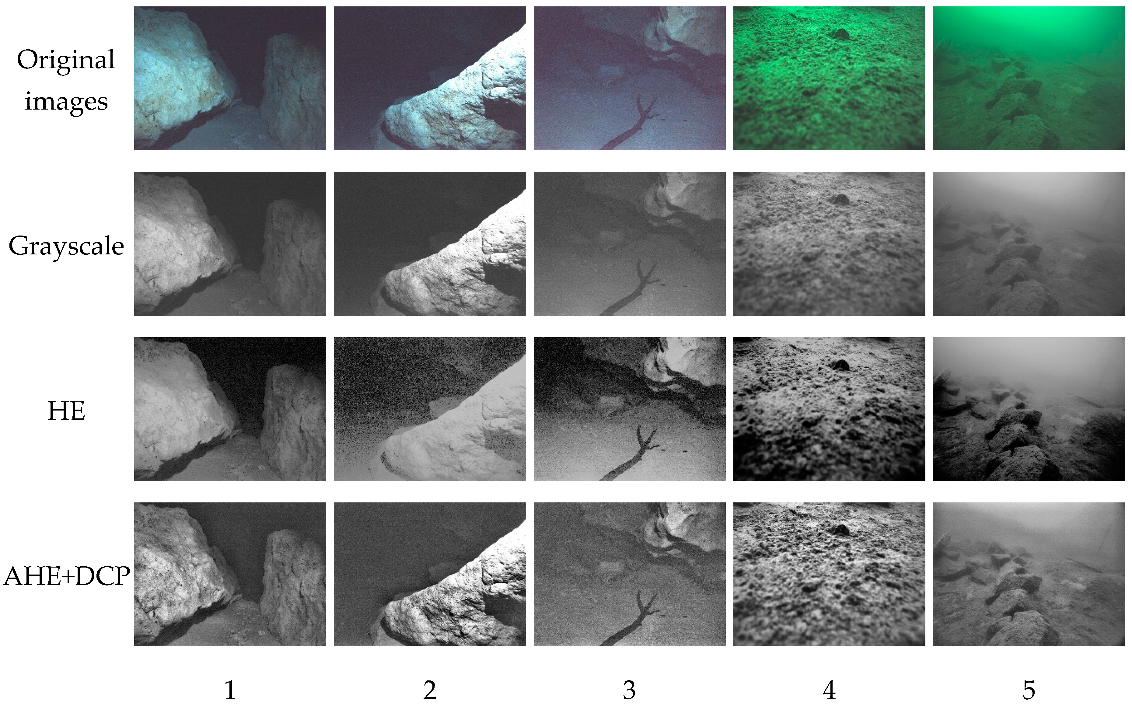
4.1. Underwater Image Brightness-Consistency Recovery
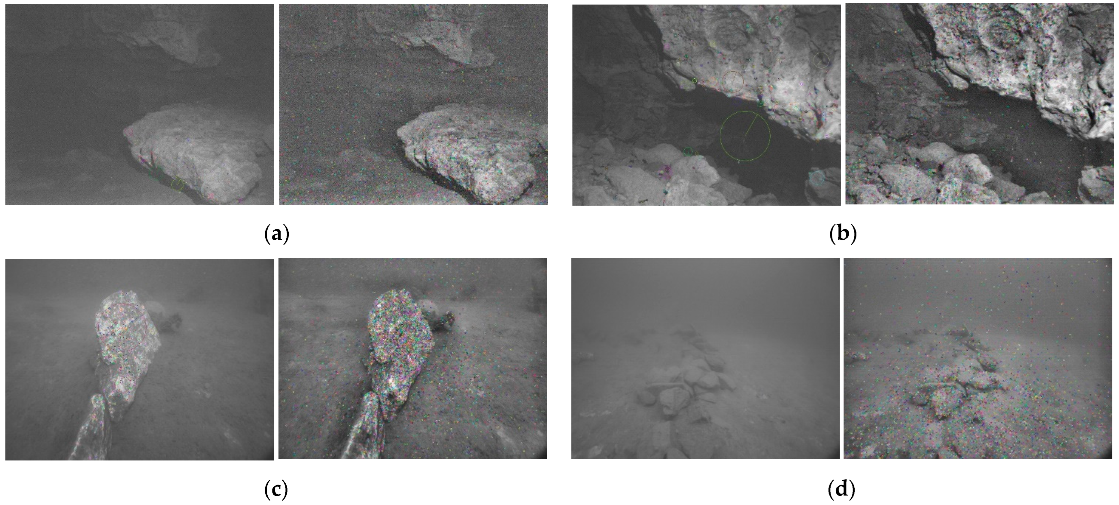
4.2. Underwater Suspended Particulate Filtration
4.3. Acoustic and Visual Feature Association for Depth Recovery
5. Results and Experiments
6. Conclusions
Author Contributions
Funding
Data Availability Statement
Acknowledgments
Conflicts of Interest
References
- Wang, X.; Fan, X.; Shi, P.; Ni, J.; Zhou, Z. An overview of key SLAM technologies for underwater scenes. Remote Sens. 2023, 15, 2496. [Google Scholar] [CrossRef]
- Davison, A.J.; Reid, I.D.; Molton, N.D.; Stasse, O. MonoSLAM: Real-time single camera SLAM. IEEE Trans. Pattern Anal. Mach. Intell. 2007, 29, 1052–1067. [Google Scholar] [CrossRef] [PubMed]
- Taketomi, T.; Uchiyama, H.; Ikeda, S. Visual SLAM algorithms: A survey from 2010 to 2016. IPSJ Trans. Comput. Vis. Appl. 2017, 9, 16. [Google Scholar] [CrossRef]
- Köser, K.; Frese, U. Challenges in underwater visual navigation and SLAM. AI Technol. Underw. Robot. 2020, 96, 125–135. [Google Scholar]
- Cho, Y.; Kim, A. Visibility enhancement for underwater visual SLAM based on underwater light scattering model. In Proceedings of the 2017 IEEE International Conference on Robotics and Automation (ICRA), Singapore, 29 May 2017–3 June 2017; pp. 710–717. [Google Scholar]
- Hidalgo, F.; Bräunl, T. Evaluation of several feature detectors/extractors on underwater images towards vSLAM. Sensors 2020, 20, 4343. [Google Scholar] [CrossRef]
- Zhang, J.; Han, F.; Han, D.; Yang, J.; Zhao, W.; Li, H. Integration of Sonar and Visual Inertial Systems for SLAM in Underwater Environments. IEEE Sens. J. 2024, 24, 16792–16804. [Google Scholar] [CrossRef]
- Leutenegger, S.; Lynen, S.; Bosse, M.; Siegwart, R.; Furgale, P. Keyframe-based visual–inertial odometry using nonlinear optimization. Int. J. Robot. Res. 2015, 34, 314–334. [Google Scholar] [CrossRef]
- Qin, T.; Li, P.; Shen, S. Vins-mono: A robust and versatile monocular visual-inertial state estimator. IEEE Trans. Robot. 2018, 34, 1004–1020. [Google Scholar] [CrossRef]
- Geneva, P.; Eckenhoff, K.; Lee, W.; Yang, Y.; Huang, G. Openvins: A research platform for visual-inertial estimation. In Proceedings of the 2020 IEEE International Conference on Robotics and Automation (ICRA), Paris, France, 31 May–31 August 2020; pp. 4666–4672. [Google Scholar]
- Hidalgo, F.; Kahlefendt, C.; Bräunl, T. Monocular ORB-SLAM application in underwater scenarios. In Proceedings of the 2018 OCEANS-MTS/IEEE Kobe Techno-Oceans (OTO), Kobe, Japan, 28–31 May 2018; pp. 1–4. [Google Scholar]
- Ferrera, M.; Moras, J.; Trouvé-Peloux, P.; Creuze, V. Real-time monocular visual odometry for turbid and dynamic underwater environments. Sensors 2019, 19, 687. [Google Scholar] [CrossRef]
- Kim, A.; Eustice, R. Pose-graph Visual SLAM with Geometric Model Selection for Autonomous Underwater Ship Hull Inspection. In Proceedings of the 2009 IEEE/RSJ International Conference on Intelligent Robots and Systems, St. Louis, MO, USA, 10–15 October 2009. [Google Scholar]
- Miao, R.; Qian, J.; Song, Y.; Ying, R.; Liu, P. UniVIO: Unified direct and feature-based underwater stereo visual-inertial odometry. IEEE Trans. Instrum. Meas. 2021, 71, 8501214. [Google Scholar] [CrossRef]
- Palomer, A.; Ridao, P.; Ribas, D. Multibeam 3D underwater SLAM with probabilistic registration. Sensors 2016, 16, 560. [Google Scholar] [CrossRef] [PubMed]
- Suresh, S.; Sodhi, P.; Mangelson, J.G.; Wettergreen, D.; Kaess, M. Active SLAM using 3D submap saliency for underwater volumetric exploration. In Proceedings of the 2020 IEEE International Conference on Robotics and Automation (ICRA), Paris, France, 31 May–31 August 2020; pp. 3132–3138. [Google Scholar]
- Palomeras, N.; Carreras, M.; Andrade-Cetto, J. Active SLAM for autonomous underwater exploration. Remote Sens. 2019, 11, 2827. [Google Scholar] [CrossRef]
- Huang, C.; Zhao, J.; Zhang, H.; Yu, Y. Seg2Sonar: A Full-Class Sample Synthesis Method Applied to Underwater Sonar Image Target Detection, Recognition, and Segmentation Tasks. IEEE Trans. Geosci. Remote Sens. 2024, 62, 5909319. [Google Scholar] [CrossRef]
- Zhou, T.; Si, J.; Wang, L.; Xu, C.; Yu, X. Automatic Detection of Underwater Small Targets Using Forward-Looking Sonar Images. IEEE Trans. Geosci. Remote Sens. 2022, 60, 4207912. [Google Scholar] [CrossRef]
- Abu, A.; Diamant, R. A SLAM Approach to Combine Optical and Sonar Information from an AUV. IEEE Trans. Mob. Comput. 2023, 23, 7714–7724. [Google Scholar] [CrossRef]
- Cheung, M.Y.; Fourie, D.; Rypkema, N.R.; Teixeira, P.V.; Schmidt, H.; Leonard, J. Non-gaussian slam utilizing synthetic aperture sonar. In Proceedings of the 2019 International Conference on Robotics and Automation (ICRA), Montreal, QC, Canada, 20–24 May 2019; pp. 3457–3463. [Google Scholar]
- Ribas, D.; Ridao, P.; Tardós, J.D.; Neira, J. Underwater SLAM in man-made structured environments. J. Field Robot. 2008, 25, 898–921. [Google Scholar] [CrossRef]
- Joshi, B.; Rahman, S.; Kalaitzakis, M.; Cain, B.; Johnson, J.; Xanthidis, M.; Karapetyan, N.; Hernandez, A.; Li, A.Q.; Vitzilaios, N.; et al. Experimental comparison of open source visual-inertial-based state estimation algorithms in the underwater domain. In Proceedings of the 2019 IEEE/RSJ International Conference on Intelligent Robots and Systems (IROS), Macau, China, 3–8 November 2019; pp. 7227–7233. [Google Scholar]
- Rahman, S.; Quattrini Li, A.; Rekleitis, I. SVIn2: A multi-sensor fusion-based underwater SLAM system. Int. J. Robot. Res. 2022, 41, 1022–1042. [Google Scholar] [CrossRef]
- Ancuti, C.; Ancuti, C.O.; Haber, T.; Bekaert, P. Enhancing underwater images and videos by fusion. In Proceedings of the 2012 IEEE Conference on Computer Vision and Pattern Recognition, Providence, RI, USA, 16–21 June 2012; pp. 81–88. [Google Scholar]
- Barros, W.; Nascimento, E.R.; Barbosa, W.V.; Campos, M.F.M. Single-shot underwater image restoration: A visual quality-aware method based on light propagation model. J. Vis. Commun. Image Represent. 2018, 55, 363–373. [Google Scholar] [CrossRef]
- Schettini, R.; Corchs, S. Underwater image processing: State of the art of restoration and image enhancement methods. EURASIP J. Adv. Signal Process. 2010, 2010, 746052. [Google Scholar] [CrossRef]
- Vargas, E.; Scona, R.; Willners, J.S.; Luczynski, T.; Cao, Y.; Wang, S.; Yvan, R. Petillot Robust underwater visual SLAM fusing acoustic sensing. In Proceedings of the 2021 IEEE International Conference on Robotics and Automation (ICRA), Xi’an, China, 30 May–5 June 2021; pp. 2140–2146. [Google Scholar]
- Nalli, P.K.; Kadali, K.S.; Bhukya, R.; Palleswari, Y.T.R.; Siva, A.; Pragaspathy, S. Design of exponentially weighted median filter cascaded with adaptive median filter. J. Phys. Conf. Series. IOP Publ. 2021, 2089, 012020. [Google Scholar] [CrossRef]
- Çelebi, A.T.; Ertürk, S. Visual enhancement of underwater images using empirical mode decomposition. Expert Syst. Appl. 2012, 39, 800–805. [Google Scholar] [CrossRef]
- Prabhakar, C.J.; Kumar, P.U.P. Underwater image denoising using adaptive wavelet subband thresholding. In Proceedings of the 2010 International Conference on Signal and Image Processing, Chennai, India, 15–17 December 2010; pp. 322–327. [Google Scholar]
- Available online: https://afrl.cse.sc.edu/afrl/resources/datasets/ (accessed on 16 May 2024).


| Sensor | Specifications |
|---|---|
| Cameras (IDS UI-3251LE) | 15 frames per second Resolution: 1600 × 1400 |
| Sonar (IMAGENEX 831L) | Angular resolution: 0.9° Maximum detection distance: 6 m Scanning period: 4 s Effective intensity range: 6 to 255 |
| IMU (Microstrain 3DM-GX4-15) | Frequency: 100 Hz Noise density: 0.005°/s/√Hz Drift: 10°/h |
| Pressure Sensor (Bluerobotics Bar30) | Frequency: 15 Hz Maxdepth: 300 M |
| Sensor | Ros Topic | Data |
|---|---|---|
| Camera | /slave1/image_raw/compressed | Left camera image |
| /slave2/image_raw/compressed | Right camera image | |
| IMU | /imu/imu | Angular velocity and acceleration data |
| Sonar | /imagenex831l/range_raw | Acoustic image |
| Pressure sensor | /bar30/depth | Bathymetric data |
| Method | 1 | 2 | 3 | 4 | 5 | |
|---|---|---|---|---|---|---|
| HE | SNR | 8.04 dB | 6.53 dB | 9.64 dB | 6.26 dB | 6.61 dB |
| MSE | 2591.091 | 3618.180 | 1767.297 | 3846.195 | 3552.464 | |
| PSNR | 13.9961 dB | 12.5461 dB | 15.6538 dB | 12.2856 dB | 12.6368 dB | |
| Time | 0.0963 s | 0.0681 s | 0.1383 s | 0.5485 s | 0.5774 s | |
| AHE+DCP | SNR | 9.15 dB | 7.95 dB | 13.31 dB | 6.34 dB | 6.69 dB |
| MSE | 1979.318 | 2606.236 | 757.346 | 3778.759 | 3565.582 | |
| PSNR | 14.3877 dB | 13.975 dB | 19.346 dB | 12.369 dB | 12.715 dB | |
| Time | 0.0823 s | 0.0573 s | 0.1454 s | 0.5758 s | 0.5758 s |
| 1 | 2 | 3 | 4 | |
|---|---|---|---|---|
| Original Image | 103 | 351 | 806 | 2 |
| HE | 135 | 460 | 821 | 288 |
| AHE+DCP | 198 | 682 | 1125 | 523 |
| 1 | 2 | 3 | 4 | |
|---|---|---|---|---|
| Original Image | 85 | 321 | 613 | 0 |
| Enhanced Image | 125 | 456 | 746 | 233 |
| The Improved Visual SLAM Results Compared with the Ground Truth | OKVIS Results Compared with the Ground Truth | |
|---|---|---|
| max | 0.829411 | 2.627724 |
| mean | 0.366091 | 1.148321 |
| median | 0.309184 | 1.020354 |
| min | 0.077178 | 0.295083 |
| rmse | 0.420158 | 1.267575 |
| sse | 7.414390 | 93.191309 |
| std | 0.206181 | 0.536756 |
Disclaimer/Publisher’s Note: The statements, opinions and data contained in all publications are solely those of the individual author(s) and contributor(s) and not of MDPI and/or the editor(s). MDPI and/or the editor(s) disclaim responsibility for any injury to people or property resulting from any ideas, methods, instructions or products referred to in the content. |
© 2024 by the authors. Licensee MDPI, Basel, Switzerland. This article is an open access article distributed under the terms and conditions of the Creative Commons Attribution (CC BY) license (https://creativecommons.org/licenses/by/4.0/).
Share and Cite
Qiu, H.; Tang, Y.; Wang, H.; Wang, L.; Xiang, D.; Xiao, M. An Improved Underwater Visual SLAM through Image Enhancement and Sonar Fusion. Remote Sens. 2024, 16, 2512. https://doi.org/10.3390/rs16142512
Qiu H, Tang Y, Wang H, Wang L, Xiang D, Xiao M. An Improved Underwater Visual SLAM through Image Enhancement and Sonar Fusion. Remote Sensing. 2024; 16(14):2512. https://doi.org/10.3390/rs16142512
Chicago/Turabian StyleQiu, Haiyang, Yijie Tang, Hui Wang, Lei Wang, Dan Xiang, and Mingming Xiao. 2024. "An Improved Underwater Visual SLAM through Image Enhancement and Sonar Fusion" Remote Sensing 16, no. 14: 2512. https://doi.org/10.3390/rs16142512
APA StyleQiu, H., Tang, Y., Wang, H., Wang, L., Xiang, D., & Xiao, M. (2024). An Improved Underwater Visual SLAM through Image Enhancement and Sonar Fusion. Remote Sensing, 16(14), 2512. https://doi.org/10.3390/rs16142512