Abstract
Lake ice thickness (LIT) is a sensitive indicator of climate change, identified as a thematic variable of Lakes as an Essential Climate Variable (ECV) by the Global Climate Observing System (GCOS). Here, we present a novel and efficient analytically based retracking approach for estimating LIT from high-resolution Ku-band (13.6 GHz) synthetic-aperture radar (SAR) altimetry data. The retracker method is based on the analytical modeling of the SAR radar echoes over ice-covered lakes that show a characteristic double-peak feature attributed to the reflection of the Ku-band radar waves at the snow–ice and ice–water interfaces. The method is applied to Sentinel-6 Unfocused SAR (UFSAR) and Fully Focused SAR (FFSAR) data, with their corresponding tailored waveform model, referred to as the SAR_LIT and FFSAR_LIT retracker, respectively. We found that LIT retrievals from Sentinel-6 high-resolution SAR data at different posting rates are fully consistent with the LIT estimations obtained from thermodynamic lake ice model simulations and from low-resolution mode (LRM) Sentinel-6 and Jason-3 data over two ice seasons during the tandem phase of the two satellites, demonstrating the continuity between LRM and SAR LIT retrievals. By comparing the Sentinel-6 SAR LIT estimates to optical/radar images, we found that the Sentinel-6 LIT measurements are fully consistent with the evolution of the lake surface conditions, accurately capturing the seasonal transitions of ice formation and melt. The uncertainty in the LIT estimates obtained with Sentinel-6 UFSAR data at 20 Hz is in the order of 5 cm, meeting the GCOS requirements for LIT measurements. This uncertainty is significantly smaller, by a factor of 2 to 3 times, than the uncertainty obtained with LRM data. The FFSAR processing at 140 Hz provides even better LIT estimates, with 20% smaller uncertainties. The LIT retracker analysis performed on data at the higher posting rate (140 Hz) shows increased performance in comparison to the 20 Hz data, especially during the melt transition period, due to the increased statistics. The LIT analysis has been performed over two representative lakes, Great Slave Lake and Baker Lake (Canada), demonstrating that the results are robust and hold for lake targets that differ in terms of size, bathymetry, snow/ice properties, and seasonal evolution of LIT. The SAR LIT retrackers presented are promising tools for monitoring the inter-annual variability and trends in LIT from current and future SAR altimetry missions.
1. Introduction
Lake ice thickness (LIT) is a sensitive indicator of climate change recognized as a thematic variable of Lakes as an Essential Climate Variable (ECV) by the Global Climate Observing System (GCOS) of the World Meteorological Organization (WMO) [1]. LIT also plays a significant role in the economy of northern regions through its influence on transportation, travel, fishing, and recreation activities [2]. The thickness of lake ice has been decreasing with climate warming and is expected to further decrease in the foreseeable future [3]. Yet, continuous monitoring of LIT is limited as field measurements are sparse in both geographical coverage and time, and have been decreasing over the last few decades [4]. Remote sensing can help to fill this gap, ensuring global monitoring, but, to date, the number of studies exploring the potential of satellite-based LIT measurements has been limited and the GCOS requirements regarding spatial and temporal resolutions, measurement uncertainty, and stability (change in bias over time) for LIT monitoring have not been fully met. According to GCOS [1], the minimum requirement (or threshold) LIT is a spatial resolution of 10 km, temporal resolution of 365 days (measurement at the time of maximum ice thickness), uncertainty of 15 cm (in units of 2 standard deviations), and stability of 10 cm. The GCOS ECVs’ requirements document indicates that a significant improvement (or breakthrough) would be achieved with a spatial resolution of 1 km, temporal resolution of 30 days, uncertainty of 10 cm (in units of 2 standard deviations), and an unspecified stability.
A recent review of radar remote sensing of lake ice that includes a review of algorithms and future directions for the retrieval of LIT is given in [4]. In previous studies, refs. [5,6] demonstrated the high sensitivity of passive microwave brightness temperature satellite measurements to ice growth and the potential of AMSR-E’s 18.7 GHz (v-pol) channel to estimate LIT with uncertainties in the order of 20 cm on a 10 km grid (below the GCOS minimum requirement of 15 cm for uncertainty but on par with the 10 km requirement for spatial resolution). Radar altimetry currently has great potential to provide long LIT time series (20–30 years), as needed for climate monitoring at the breakthrough level defined by GCOS as indicated above. Ref. [7] showed the potential of estimating LIT from the varying peak separation, linked to the ice growth, of Cryosat-2 Ku-band synthetic-aperture radar (SAR) waveforms, but achieving RMSE values ranging from 20 cm to 41 cm when compared to in situ measurements from Great Slave Lake and Great Bear Lake, Canada. More recently, ref. [8] proposed improving this approach by using ICESat-2 data to increase the accuracy of the Cryosat-2 peak selection, obtaining LIT estimates with an RMSE of 0.14 cm when compared to field measurements. It is worth noting here that assessing the accuracy of satellite-based LIT retrievals by using in situ measurements can be somewhat misleading as these are usually collected operationally near the shore of the lakes, while the satellite ground track segments used for the LIT estimates are taken over the lakes, far away from the shore, to avoid land contamination. Care should therefore be taken when evaluating along-track satellite altimetry retrievals of LIT against in situ measurements since the snow/ice properties and ice thickness can be quite different over distances that can be of the order of several tens of kilometers between the two sets of measurements.
Other recent studies [9,10,11,12] have exploited radar waveforms for LIT estimation from different missions (both low-resolution mode or LRM, and SAR mode), mainly focusing on the estimation of the bias introduced by the presence of ice in winter on lake water level (LWL) measurements, more than on obtaining an accurate LIT estimation. Additionally, the studies mentioned above make use of empirical methods and/or retrackers that cannot correctly account for the specific waveform shape over ice-covered lakes and also depend on threshold settings that are not accurate enough to follow the LIT evolution, in particular, at the seasonal transitions when the LIT signature is less discernible in the radar waveforms, leading to biased and sub-optimal LIT estimation. Significant improvements in LIT estimation have recently been reported by [13] through the implementation of a physical-based analytical retracker for the analysis of Ku-band LRM waveform data. The method provides a robust way to assess the accuracy of LIT retrievals that does not rely on in situ measurements. It provides estimates of LIT with an uncertainty of the order of 10 cm. Also, ref. [13] demonstrated the capability of the analytical retracker to consistently capture the seasonal transitions of LIT during the freeze-up and break-up periods and ice growth over different winter seasons, making it a powerful and promising tool for monitoring the inter-annual variability and trends in LIT. The method has recently been implemented within the ESA Lakes_cci project (https://climate.esa.int/en/projects/lakes/, accessed on 28 June 2024) to generate long (20+ years) LIT time series from radar altimetry over different lake targets. The LIT time series are publicly available through the project portal according to the data release schedule. While [13] paved the way towards fulfilling the ambitious GCOS requirements for LIT, further improvements can still be achieved by using data at higher spatial resolution, that is, SAR altimetry data.
In this paper, we present a novel LIT analytical retracker tailored for the analysis of Ku-band SAR waveforms from both unfocused (UFSAR) [14] and fully focused (FFSAR) [15] modes that allows for a robust estimation of LIT and that significantly improves the precision of LIT retrievals with respect to previous studies, opening the possibility of accurate LIT monitoring from current and future SAR altimetry missions. The paper focuses on the analysis of Sentinel-6 SAR data, publicly available, at nominal 20 Hz sampling. It also explores the benefit for LIT analysis of processed Sentinel-6 data at a higher posting rate (140 Hz) for both UFSAR and FFSAR modes. The SAR LIT analysis is evaluated through comparison with LIT thermodynamics model simulations [16] and LIT estimates obtained from Sentinel-6 and Jason-3 LRM data for the same lake targets and dates, during the tandem phase of the two satellites. Assessing the consistency between SAR-based and LRM-based LIT retrievals is important to ensure the continuity of the measurements issued from past, current and, eventually, future radar altimetry missions for climate monitoring.
The paper is organized as follows. Section 2 describes the LIT signature in Ku-band SAR waveforms in the case of UFSAR at 20 Hz as well as UFSAR and FFSAR at 140 Hz, showing how the signal evolves during a typical ice season. Section 3 presents the mathematical formalism of the SAR_LIT and FFSAR_LIT retrackers, detailing the analytical modeling of the SAR radar waveforms with the LIT signature for UFSAR and FFSAR data, and describing the parameter estimation method. Details on the Sentinel-6 system and sensor settings used in the retrackers are given in the Appendix A. Section 4 presents the altimetry data used for the LIT analysis and the thermodynamic lake ice model simulations. It also describes the target lakes considered. Section 5 describes the results and assessment of the LIT analysis. Finally, Section 6 summarizes the key findings of the study and provides avenues for future research.
2. Lake Ice Thickness Signature in SAR Radar Echograms and Waveforms
The presence of snow and ice modifies the propagation of the radar waves, and their penetration depends on the frequency of the incident signal and the properties of the different layers crossed. In the case of Ku-band (12–18 GHz), a specific signature is observed in radar altimetry waveforms consisting of a step-like break on the leading edge of LRM waveforms (see, e.g., [13]) and a double peak in high-resolution SAR waveforms in both unfocused and fully focused modes (see, e.g., [7,9] for UFSAR). The width of the step and the separation between the two peaks, respectively, is directly linked to LIT. This specific signature is related to the double backscattering of the radar waves at (i) the snow–ice interface and (ii) the ice–water interface [7,17], which is particularly noticeable in the case of dry snow overlaying clear freshwater ice. In this paper, we focus on the analysis and modeling of high-resolution radar waveforms data (UFSAR and FFSAR) over ice-covered lakes, with the aim of exploiting the double-peak signature to obtain robust LIT estimates of higher accuracy compared to those retrieved from LRM data and in previous studies that make use of empirical methods (as, e.g., [7,8,9,10]).
An illustrative example of the evolution of the double-peak signature related to LIT in the case of 20 Hz Sentinel-6 UFSAR data from Great Slave Lake, Canada, is provided in Figure 1. The plots in the left column of the figure show Sentinel-6 UFSAR echograms, while those in the right column display the corresponding stacked waveforms, with, in black, the mean waveform at different periods: at the beginning of the ice season in December 2021 (top row), when the ice is well established on the lake in February 2021 (second row), when the ice is still present but the snow/ice interface is less discernible at the end of April 2021 (third row), and at the beginning of the melt period in May 2021 (bottom row). As can be seen in the figure, the LIT signature in radar waveforms evolves according to changes in the snow and ice conditions and thickness during the ice season. In December, the ice is thin and heterogeneous over the RoI, the peak separation is small with a slightly smaller amplitude of the first peak. In February, when the ice is well established on the lake, the bimodal signature is clearly visible and the two peaks have a comparable amplitude. At the end of April, the double-peak signature is again less perceptible, with a lower amplitude for the first peak. Finally, in mid-May, the bimodal feature is no longer present and this is likely due to the fact that surface (snow) melt has begun, which leads to a highly reflective surface where the two interfaces are no longer discernible. These features are in line with the ESA LIAM project (https://www.h2ogeomatics.com/lake-ice-from-altimetry-missions-li, accessed on 28 June 2024) findings that support the lack of a peak at the start of the season, then a bigger step as the season progresses and snow is more prominent, then, later in the season, a loss of the peak. This evolution is primarily tied to the surface roughness but more exploratory work is needed to confirm this aspect of the waveform.
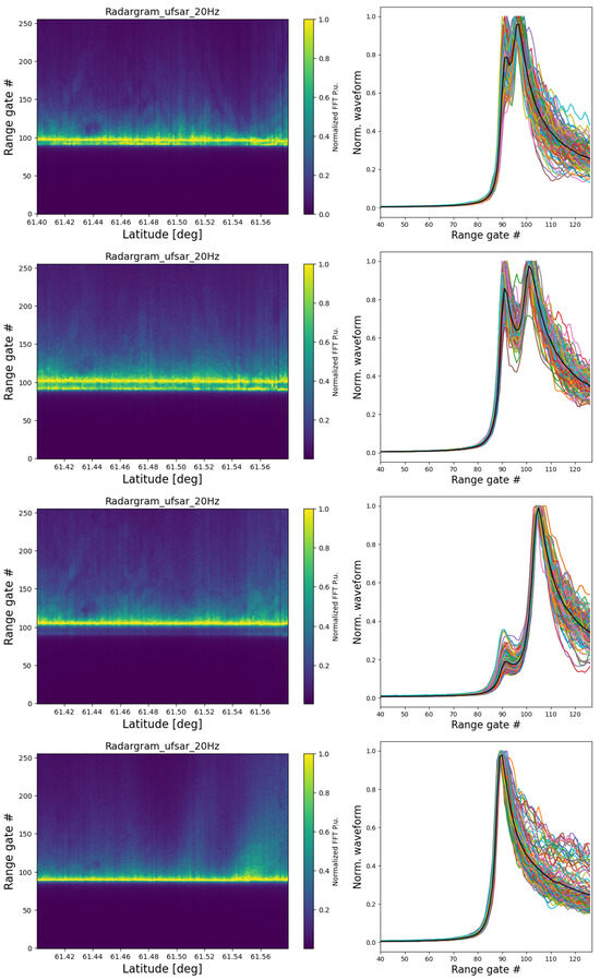
Figure 1.
Illustration of the evolution of the bimodal lake ice thickness signature in Sentinel-6 UFSAR radargrams (left column) and the normalized waveforms (right column) at 20 Hz resolution at Great Slave Lake in December 2021 (top), February 2021 (second row), end of April 2021 (third row), and May 2021 (bottom). The black line in the plots of the right column corresponds to the mean waveform in the selected region of the lake.
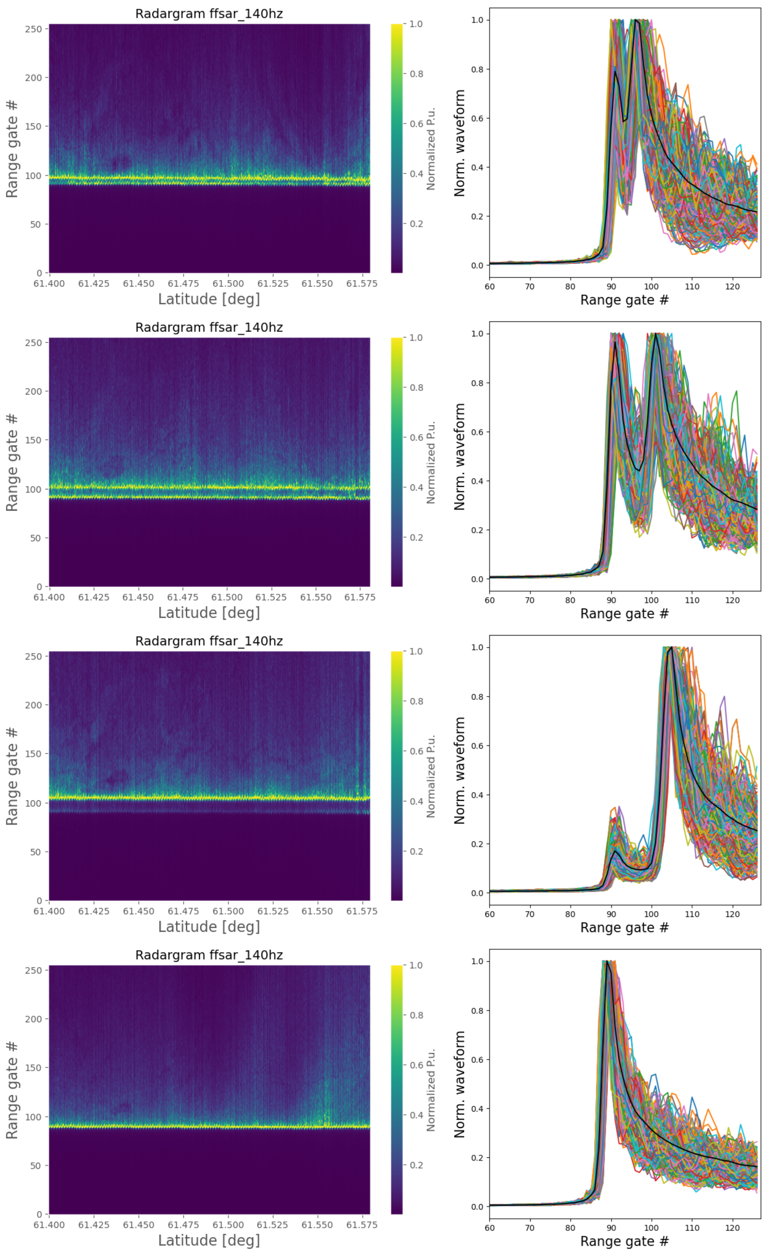
The radargrams of the 140 Hz rate Sentinel-6 FFSAR data for the same lake target and dates are shown in Figure 2, revealing similar features as the UFSAR radargrams of Figure 1 but with increased resolution. The evolution of the LIT signature, being related to the properties of the lake surface, is visible in both the UFSAR and FFSAR radargrams. The two peaks on the leading edge of the FFSAR waveforms appear, however, to be better resolved compared to those from UFSAR, suggesting possible improvements to be gained in the retrieval of LIT. Also, radar backscatter from off-nadir water surfaces is more clearly observed on the trailing edge of the Sentinel-6 FFSAR waveforms, better reflecting the complex nature of the surface within the radar footprint. This information can be very useful, for example, in gaining better insight into the evolution of LIT, especially in the seasonal transition, when the surface is not homogeneous.
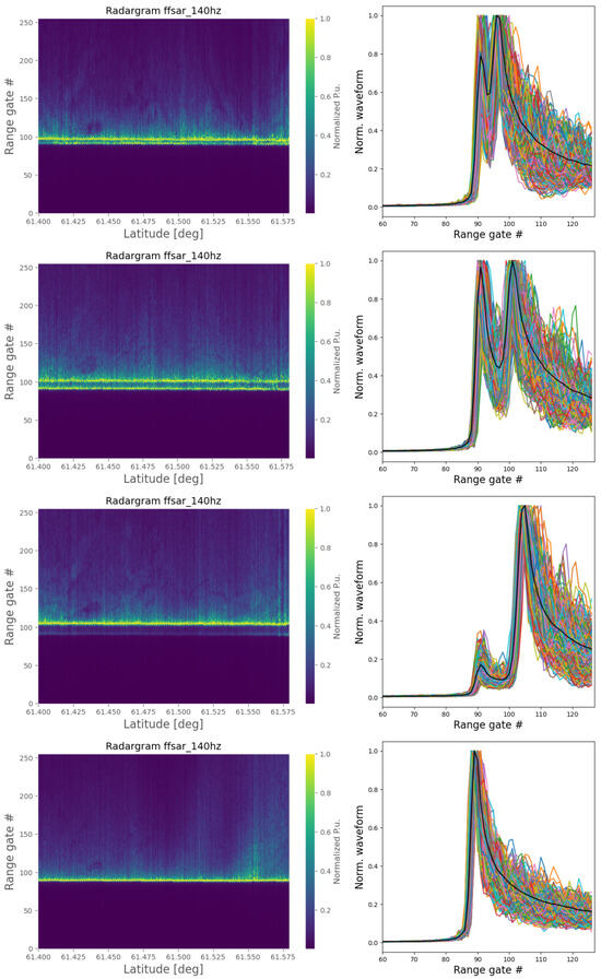
Figure 2.
Illustration of the evolution of the bimodal lake ice thickness signature in Sentinel-6 FFSAR radargrams (left column) and the normalized waveforms (right column) at 140 Hz posting rate at Great Slave Lake in December 2021 (top), February 2021 (second row), end of April 2021 (third row), and May 2021 (bottom). The black line in the plots of the right column corresponds to the mean waveform in the selected region of the lake.
Given the specific LIT signature in the high-resolution Ku-band SAR waveforms described above, we developed a retracking approach based on the physical modeling of the signal and specific for the detection of LIT that allows for the analytical modeling of the LIT signal and its evolution in the case of UFSAR and FFSAR waveforms, as detailed in the following section.
3. Analytical Retrackers for the Estimation of LIT from High-Resolution SAR Data
In this section, we provide details on the analytical retrackers developed to estimate LIT from the UFSAR and FFSAR data that are referred to hereafter as the SAR_LIT retracker and the FFSAR_LIT retracker, respectively.
3.1. SAR_LIT Waveform Model
In order to reproduce the double-peak signature related to LIT, the SAR waveform of ice-covered lakes can be analytically modeled as the sum of two SAR waveforms. Making use of the formalism of [18,19], the resulting radar waveform for a single beam, , and as a function of the range gate bin x and the parameter vector , takes the following form (because the analysis is specific to ice-covered lakes, the significant wave height (SWH) is assumed to be zero, and therefore, in the following, we assume that the terms related to SWH can be neglected):
where is the look angle for the ℓ beam,
is the parameter related to the amplitude of the first peak, is the amplitude of the second peak, and
where is the central gate, corresponding to the epoch of the first echo, is the ice thickness parameter (in unit of range gates) that quantifies the peak separation. In the case of ice-covered lakes, the term related to the significant wave height can be neglected, and the term can be approximated by
where is the PTR bandwidth in range gate unit, and
with
where h is the nominal orbit height, is the Earth’s radius, is the along track resolution and is the vertical resolution, respectively, defined as
with the sampling frequency, c the speed of light, the pulse repetition frequency, the nominal satellite velocity, the center frequency, and the number of pulses per burst. Following [19], the function can be expressed analytically as
with and
with the modified Bessel function of the first kind and order . In the case of no mispointing (), the function can be written as
where is the attenuation parameter defined as the inverse of the mean square slope parameter s as in [19], and
with and the half-power beam widths, along track and across track, respectively.
Finally, the multi-look SAR waveform over ice-covered lakes takes the form
where L is the total number of Doppler beams and is the parameters vector:
Equation (15) defines the SAR_LIT retracker’s waveform model. The values of the parameters related to the instrument in the SAR_LIT retracker model for Sentinel-6 [20] used for the analysis of the SAR data from this mission are reported in Table A1. The ice thickness, , in units of meters, is defined by applying the following conversion from range gates to meters:
where is the sampling frequency, and is the speed of light in the ice, with c the speed of light in the vacuum and the refractive index of ice (=1.7861). Note that a factor of four appears in the denominator of Equation (17), accounting for the factor of two related to the travel time and the factor of two related to the range gate oversampling of the SAR waveform.
3.2. FFSAR_LIT Waveform Model
The FFSAR LIT waveform model shares the same formalism described in Section 3.1. However, for the Sentinel-6 mission, the FFSAR model is less complex and more computationally efficient than that for UFSAR. Unlike missions operating in closed-burst mode (or lacunar sampling) such as Cryosat-2 and Sentinel-3, the Sentinel-6 altimeter uses an interleaved measurement mode (open-burst mode) that significantly reduces the level of grating lobes in the Sentinel-6 FFSAR impulse response [15,20]. Consequently, the Sentinel-6 FFSAR waveforms are narrower than UFSAR waveforms and can be retracked with the zero-Doppler UFSAR beam model, as reported in [21]. The analytical formulation of the Sentinel-6 FFSAR waveform model is thus given by the single-looked echo of the central beam , taking the form
where is given in Equation (1). This formulation is not valid for missions operating in closed-burst mode. Their grating lobes are strong and distort the altimeter’s impulse response, which makes the FFSAR waveforms resemble those of UFSAR, thus giving them similar resolution. In this case, the FFSAR waveform model can be directly emulated from the UFSAR model [21].
3.3. Parameter Estimation
The parameter estimation method is chosen with the goal of building consistent LIT time series with the associated uncertainty that can be exploited for LIT climatology. For this purpose, for each data cycle over a target lake, the LIT retracker analysis, for both UFSAR and FFSAR, is performed within a region of interest (RoI) defined as a segment of the satellite ground track with a latitude cut chosen to minimize land contamination, thus consisting in the part of the track furthest from the shore, and sufficiently large to include enough statistics to obtain robust and reliable estimates. The LIT analysis consists of two steps: (1) the optimization step, that is, the retracker analysis, involving the waveform fit with the corresponding LIT waveform model; and (2) the estimation of the parameters’ means and standard deviations.
The optimization step consists in performing a least square Levenberg–Marquardt weighted fit of each waveform in the chosen RoI with the waveform model described in Section 3. As in [13], the weights are defined as the data variance within the RoI, ensuring an optimal parameter estimation (it can be demonstrated that in the case of a Gaussian likelihood function, a weighted least square estimator with weights defined as the data (co)variance, is equivalent to a maximum likelihood estimator, thus providing an optimal parameter estimation). In practice, the function to be minimized is
where is the vector of residuals between the data, , and the waveform model , and is the diagonal noise covariance matrix, with computed as the standard deviation of the echoes within the LIT analysis window. Weighting the fit by allows for the waveform noise to be accounted for.
The second step of the retracking analysis is the parameter estimation, which provides, as the main output, the LIT estimate with the associated uncertainty. The estimation is performed by computing the mean and standard deviation of the fitted parameters for each overpass (data cycle) in the RoI. To obtain the parameter constraints with the corresponding uncertainties, for each data cycle, the histograms of the five fitted parameters are computed and a Gaussian fit provides the mean and standard deviation for each parameter. In order to exclude possible outliers, data editing is applied before computing the histograms, selecting the physical LIT values < 4 m and the LIT estimations within a window of 1 m centered on the mean, which is a conservative choice considering that, for a conservative LIT uncertainty around 15 cm, this corresponds to a window centered within ~3.
The LIT uncertainty, being calculated as the standard deviation of the LIT estimates in the LIT analysis window over the target lake, includes contributions related to the retracked radar waveform’s noise and the spatial variation in the LIT estimates within the RoI. In the case of homogeneous ice cover, the dispersion of the LIT measurements (i.e., the width of the histogram) is essentially due to the waveform noise, as is typically the case in the middle of the ice season when the ice is well established and the spatial variations in LIT are small. However, at the seasonal transitions, when the ice is initially forming or is melting, the lake surface is no longer homogeneous, leading to significant variability in the LIT signature in the radar waveforms. This translates into significant spatial variation in the retrieved ice thickness which dominates the error budget, resulting in an increased uncertainty in LIT with respect to the uncertainty expected when considering the waveform noise contribution only.
4. Target Lakes and Data
The lakes selected for the LIT analysis are described in Section 4.1. The data used for the LIT analysis are high-resolution UFSAR and FFSAR mode data from the Sentinel-6 mission (Section 4.2.1) and LRM data from the Sentinel-6 and Jason-3 missions (Section 4.2.2). The analysis is performed over two ice seasons (2020–2021 and 2021–2022) during the tandem phase of the Sentinel-6 and Jason-3 satellites (December 2020 to April 2022) to ensure the consistency of the LIT estimates between the two missions, and also to assess the continuity between the LRM and SAR modes for the estimation of LIT. The thermodynamic ice model simulations of LIT time series [16] used for comparison with estimates from the retrackers are described in Section 4.3. It should be noted that in situ LIT measurements are not used for the validation of radar altimetry LIT estimates; no measurements are available for Great Slave Lake during the study period and the few from Baker Lake were collected close to the shore by local authorities at a distance of 30 km from the altimeter track (Figure 3). As previously indicated by [13], in situ LIT measurements gathered as part of the environmental monitoring programs of government agencies are usually taken near the lake shores, while the retrievals from altimetry are performed using data from a segment of the satellite’s ground track chosen to be far away from the shore to avoid land contamination, thus a very different location in terms of bathymetry, wind exposure, snow coverage, and depth. These factors play a significant role on the timing of ice formation and the evolution of ice thickness, and this can lead to LIT differences on the order of tens of centimeters (e.g., [16,22]), making in situ data of limited use for a precise validation of the satellite-based LIT estimates.
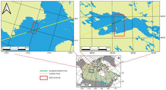
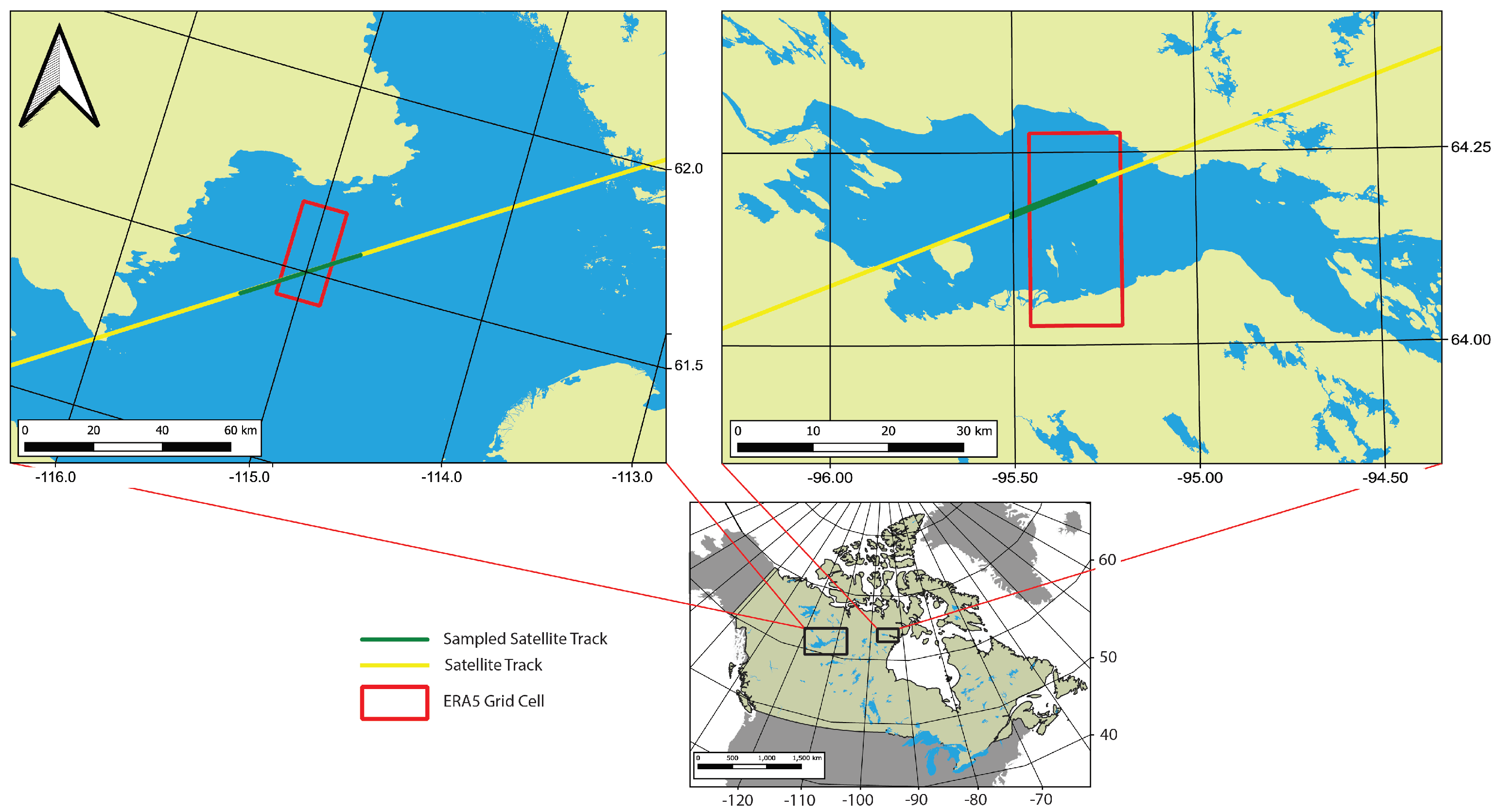
Figure 3.
The target lakes of the LIT analysis, Great Slave Lake and Baker Lake, Canada, are shown on the map (bottom) and with the satellite ground tracks superimposed on the lakes (upper left and right, respectively).
4.1. Target Lakes
The two target lakes selected for the LIT analysis are Great Slave Lake and Baker Lake, both located in the subarctic continental climate zone of Canada (Figure 3). Great Slave Lake is the second largest lake in Canada, covering an area of ≃28,000 km2, with mean and maximum depths of 41 and 614 m, respectively. Baker Lake is located at a higher latitude (64°09′N) than Great Slave (61°40′N), it is also smaller, covering an area of ≃1887 km2, thus making it a more challenging target for LIT estimation with altimetry data, in particular in LRM, because of the unavoidable land contamination given the size of the footprint which is on the order of 10 km for LRM data. The two lakes are characterized by different environmental conditions that lead to varied snow and ice properties and evolution, making them interesting case studies for the LIT analysis. It is important to note that there are missing data in the SAR HR mode for several cycles over Baker Lake during the first ice season considered for the LIT analysis (2020–2021). This is due to the fact that at the beginning of the mission, the operational acquisition mode was set to LRM with specific masks that included Baker Lake.
4.2. Altimetry Data
4.2.1. High-Resolution Data
The Sentinel-6 UFSAR waveform data at 20 Hz are provided by the Payload Data Acquisition and Processing (PDAP) component of the mission ground segment and are publicly available. Additional Sentinel-6 UFSAR and FFSAR waveform data were generated at a higher posting rate (140 Hz) using an updated version of the SMAP code [23], to assess the potential improvements brought by these new Doppler processing configurations on the LIT estimation. By increasing the posting rate of the altimeter observations beyond the standard 20 Hz, which corresponds on the ground to the UFSAR altimeter resolution, more measurements are made along the satellite track to possibly extract more information. The along-track ground spacing is reduced from 350 m to 50 m. However, in contrast to FFSAR, the spatial resolution of the UFSAR data remains unchanged and is equal to that of the 20 Hz UFSAR whatever the posting rate used.
4.2.2. Low-Resolution Data
The data used in the analysis are the 20 Hz LRM waveform data from the Jason-3 mission (SGDR L2 products available from the Aviso+ portal (https://www.aviso.altimetry.fr/, accessed on 28 June 2024)) and the Sentinel-6 PDAP LRM waveform data provided by the Sentinel-6 ground segment, which are also publicly available.
4.3. Lake Ice Model Simulations
Lake ice models provide an alternative to in situ measurements that are scarce in space and in time. Such models are particularly valuable for the development of new remote sensing-based LIT retrieval algorithms and their evaluation since in situ measurements that match the timing and locations of overpasses are most often not available or limited in terms of coverage (i.e., area covered and temporal frequency of measurements). Using lake ice models, ice thickness can be simulated on a daily basis for areas of differing water depth, snow density, and snow depth. The Canadian Lake Ice Model (CLIMo, [16]) has been used regularly in development of remote sensing algorithms as well as interpreting remote sensing signals [6,17,24,25,26]. CLIMo has also been used to investigate the impact of contemporary and future climate conditions on ice phenology (freeze-up, break-up, and ice duration), LIT, and the types of ice (snow ice and clear ice) (e.g., [3,22,27]). CLIMo is used in this study to simulate LIT for comparisons with retrievals from the altimetry data for the areas of Great Slave Lake and Baker Lake highlighted in Figure 3. CLIMo is a 1-D thermodynamic ice model and is forced using meteorological variables that can be provided from weather stations, atmospheric reanalysis, or climate model gridded products. Input data for CLIMo is provided daily and consists of 2 m air temperature, relatively humidity, cloud cover, wind speed, and snowfall (or snow depth from a nearby land site when available). Additionally, a fixed mixed layer depth and average snow density is required for the lakes of interest. The outputs from CLIMo include energy/radiation balance components, on-ice snow depth (both accumulation and melt), the temperature profile at specified depths within the snow/ice, and ice thickness. The model also provides the freeze-up and break-up dates for the lake of interest.
For this study, 2 m air temperature, wind speed, relative humidity, and cloud cover were retrieved from the ERA5 atmospheric reanalysis product from the European Centre for Medium-Range Weather Forecasts (ECMWF). Snow depth data were not used from ERA5 and were instead acquired from Environment and Climate Change Canada weather stations on the shores of GSL and Bake Lake. For GSL, the Hay River weather station was used (115.78°W, 60.84°N) and for Baker Lake the Baker Lake station was used (96.08°W, 64.3°N). Simulations were performed for the years corresponding to the altimetry acquisitions, with a mixing depth of 30 m for GSL and 20 m for Baker Lake. Average snow density for GSL was set to 300 kg m−3, which has been used for previous simulations of this lake (e.g., [6]). For Baker Lake, simulations were run at varying snow densities (200, 250, 300, and 350 kg m−3) as fewer past simulations have been conducted for this lake and this will account for variations in the snow cover. To account for variations in snow drifting on the lake ice surface CLIMo was run with four sets of snow depth scenarios: no snow, 25, 50, and 75%. From the simulation results, on-ice snow depth, ice thickness, and melt onset were retained to evaluate the estimates obtained from the altimetry data. From past simulations of LIT using CLIMo, RMSE values have been reported between 5 and 17 cm when compared to in situ measurements collected near Yellowknife [22,26]; similar errors are expected in this study.
5. Results and Discussion
This section presents the results of the LIT analysis performed with the data described in Section 4. The results focus on the LIT retrievals obtained with the SAR_LIT retracker applied to the Sentinel-6 UFSAR data at 20 Hz, which are compared to the LIT estimates obtained with Sentinel-6 data at higher resolution, that is, the UFSAR and FFSAR data processed at 140 Hz (Section 5.1). The assessment of the SAR_LIT analysis, consisting of the comparison with the LIT analysis performed on LRM data from both Sentinel-6 and Jason-3 missions and with the output of the thermodynamic CLIMo simulations of the same targets and periods, is presented in Section 5.2. Consistency checks of the LIT retrievals from radar altimetry with satellite images are also shown in this section.
5.1. LIT Analysis of Sentinel-6 High-Resolution Data
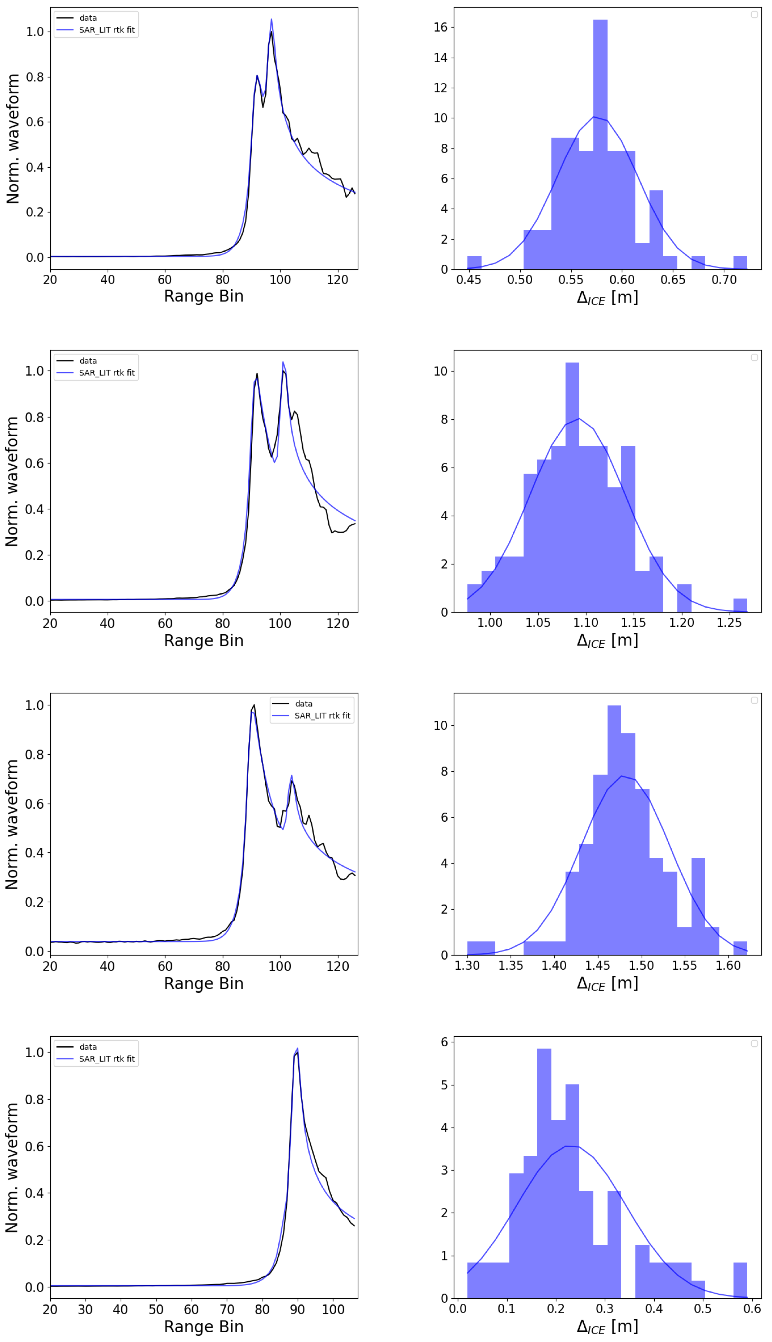
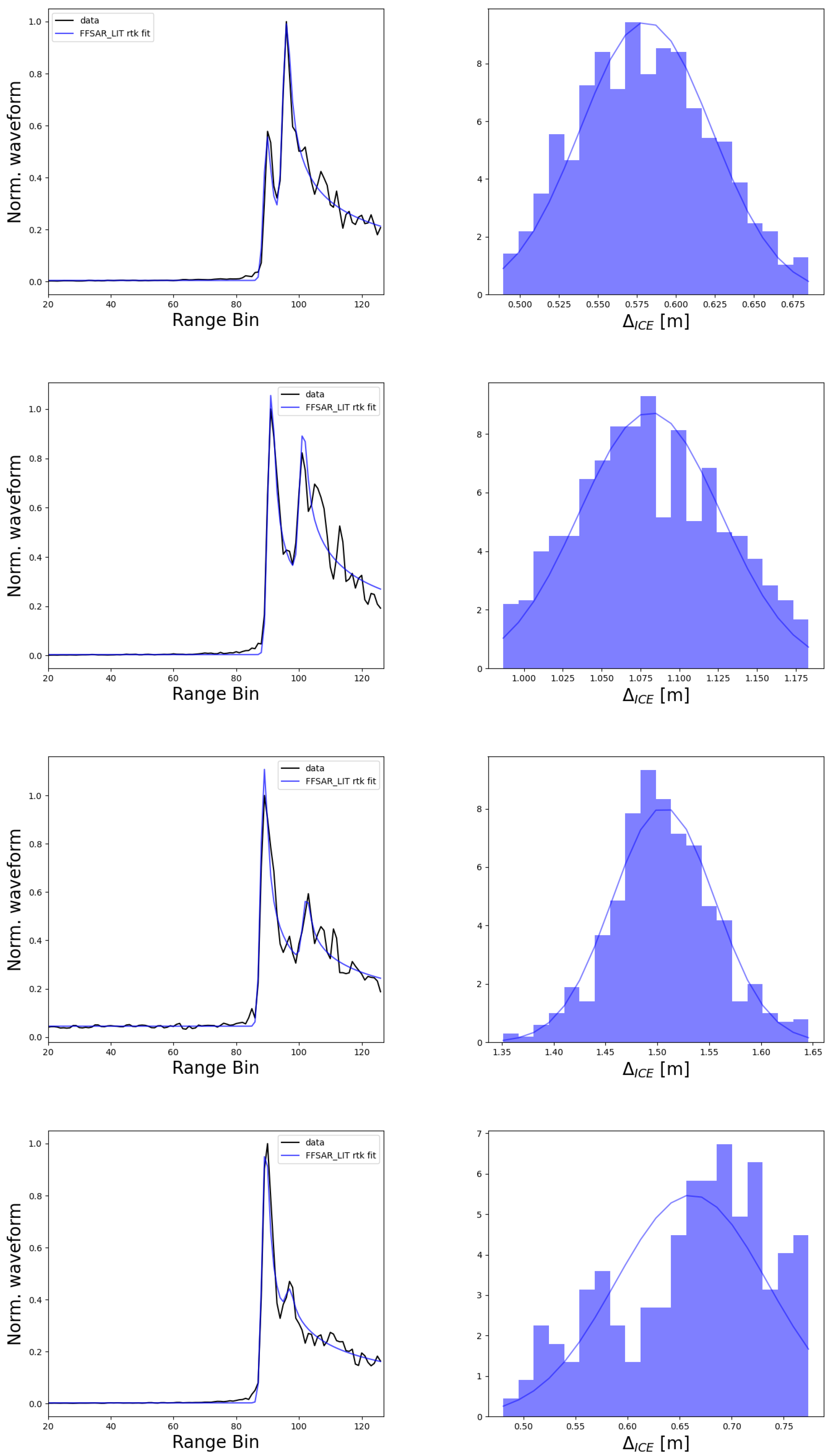
An illustrative example of the SAR_LIT analysis of high-resolution Sentinel-6 UFSAR data at 20 Hz and of the FFSAR_LIT analysis of Sentinel-6 FFSAR data at 140 Hz for Great Slave Lake during the 2020–2021 ice season is given in Figure 4 and Figure 5, respectively. Examples of Sentinel-6 waveform data (in black) with, in blue, the SAR_LIT fit (Figure 4) and the FFSAR_LIT fit (Figure 5) are shown in the left columns. In both figures, from top to bottom the plots correspond to December 2020, February 2021, April 2021, and mid-May 2021. The evolution of the bimodal LIT signature is clearly visible in the UFSAR and FFSAR waveforms, starting with a small peak separation during the ice formation period, which increases through the winter, indicating thickening of the ice, and then, disappears at the beginning of the melt period in May 2021 in the case of UFSAR data. The signature is still present on the same date on most of FFSAR waveforms, as shown in the bottom left panel of Figure 5, allowing the melting transition to be followed for longer than with UFSAR data because of the higher spatial resolution. The plots in the right column of Figure 4 and Figure 5 show the histograms of the LIT measurements obtained with the SAR_LIT and the FFSAR_LIT retrackers, respectively, in the same lake RoI and on the same dates. The blue curve corresponds to the Gaussian fit of the histograms. The changes in the histograms’ distributions and means reflect the evolution of the ice thickness within the considered region and during the ice season. The LIT standard deviation ranges from 3.6 cm to 5.9 cm for UFSAR and from 2.99 to 5.06 for FFSAR, during the ice season. During the melt period, the LIT uncertainty is bigger, on the order of 15 cm for UFSAR and 9 cm for FFSAR, due to the limited penetration depth of the signal and higher spatial variation in the ice surface within the RoI. In fact, because of the melting snow/ice, most of the UFSAR waveforms do not contain the LIT signature any longer (as in the bottom left plot example in Figure 4); yet, some waveforms still have it, as the ice is still present and the melting is not homogeneous over the considered region. In this case, the spatial variation of the LIT is higher, thus resulting in a higher standard deviation of the LIT measurements within the RoI. This holds true also for FFSAR but to a smaller extent as the lake surface is more homogeneous within the reduced FFSAR footprint and the LIT signature is present and detected for a longer period during the melting transition with respect to the UFSAR, as mentioned above.

Figure 4.
Examples of Sentinel-6 UFSAR waveform with, in blue, the SAR_LIT fit (left column) and LIT histograms, with the corresponding Gaussian fits (right column), in the RoI of Great Slave Lake at the end of December 2020 (top row), in February 2021 (second row), in April 2021 (third row), and mid-May 2021 (bottom row).
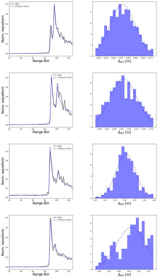
Figure 5.
Examples of Sentinel-6 FFSAR waveforms with, in blue, the FFSAR_LIT fit (left column) and LIT histograms, with the corresponding Gaussian fits (right column), in the RoI of Great Slave Lake at the end of December 2020 (top row), in February 2021 (second row), in April 2021 (third row), and mid-May 2021 (bottom row).
Similar performances and behavior of the LIT evolution are obtained for Baker Lake. A representative example showing the spatial evolution of LIT from UFSAR at 20 Hz data at Great Slave and Baker lakes in February 2021 is given in the left and right upper plots of Figure 6, respectively. The gray lines in the bottom panels show the evolution of the reduced statistics (Equation (19)) at the best fit, providing a goodness of fit metric. The fit performances are good for both lake targets, showing an overall reduced of one, meaning that the model and the data are in agreement within the variance. It can be noted that for Baker Lake there are less data points in contrast to Great Slave Lake, as it is a smaller lake, and thus, the ground track segment considered for the LIT analysis is shorter (see Figure 3), including only ~40 waveforms instead of ~120 waveforms in the RoI of Great Slave. This shows the limitation of building reliable LIT time series from small target lakes by using 20 Hz data. A possible solution to overcome this limitation is to perform the LIT analysis on the mean waveform in the RoI, instead of fitting the individual waveforms. Yet, if the number of exploitable waveform data is too small (<10/20 waveforms) this could also lead to less robust LIT estimates. Another possibility is to process the data at a posting rate higher than 20 Hz to increase the statistics, as shown, for instance, in [19,28]. With respect to this, performing the LIT analysis on Sentinel-6 SAR data processed at 140 Hz has indeed the advantage of increasing the number of waveforms in the RoI, and thus, the spatial sampling of the surface, by a factor of seven in comparison to the 20 Hz data. An illustrative example of the LIT spatial evolution obtained from FFSAR data at 140 Hz at the Great Slave and Baker lakes in February 2021 is given in the left and right bottom plots of Figure 6, respectively. The increased spatial sampling with respect to the LIT estimations obtained with the UFSAR data at 20 Hz (showed in the upper row plots of Figure 6) is clearly visible. Also, because of the higher resolution of the FFSAR data, the estimation of the LIT uncertainties is improved, yielding, for Great Slave Lake, = 1.081 ± 0.045 m, ~%10 better than the UFSAR at 20 Hz LIT estimation = 1.091 ± 0.05 m. For Baker Lake the FFSAR LIT estimation is = 1.232 ± 0.045 m, ~35% better than the 20 Hz UFSAR estimation of = 1.223 ± 0.063 m. The performances of the FFSAR_LIT retracker are good for both the lakes, with a reduced around one, as shown by the gray lines in the bottom panels of Figure 6.
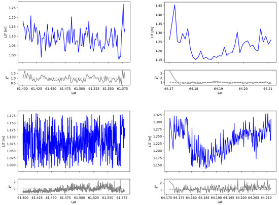
Figure 6.
Example of the spatial evolution of the LIT estimates at Great Slave Lake (left column) and Baker Lake (right column) in February 2021. The top row plots show the results for the Sentinel-6 UFSAR data at 20 Hz, while the bottom row plots for the Sentinel-6 FFSAR data at 140 Hz. The gray lines in the bottom panels of the figures show the evolution of the reduced goodness of fit metric.
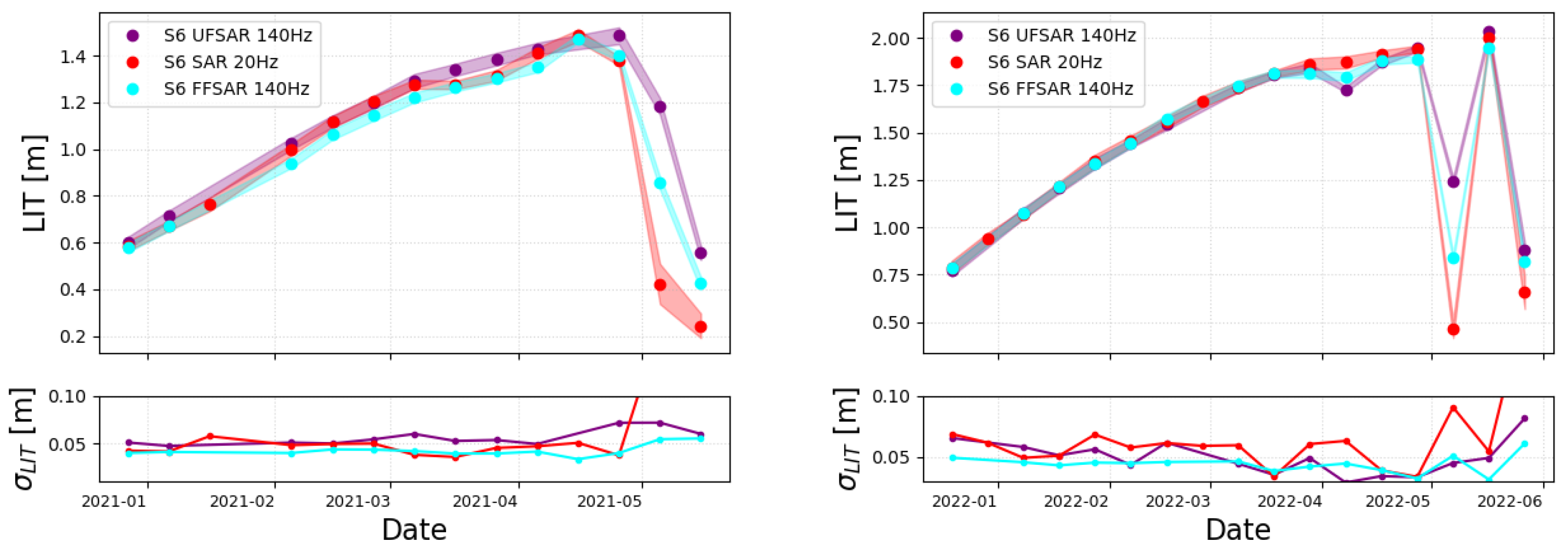
Figure 7 shows representative results of the LIT estimation obtained with high-resolution Sentinel-6 data for a complete ice season at Great Slave (left plot) and Baker (right plot) lakes. The red circles correspond to the LIT estimates obtained with the Sentinel-6 UFSAR data at 20 Hz, the purple circles to the UFSAR data at 140 Hz, and the cyan circles to the FFSAR data at 140 Hz. The shaded regions in the upper panels and the lines in the bottom panels correspond to the LIT 1 uncertainties. Overall, there is a good consistency in the LIT estimates obtained with the three datasets for both lake targets. As shown in Table 1, the mean bias error (MBE) and the root mean square error (RMSE) of Sentinel-6 UFSAR at 20 Hz and FFSAR at 140 Hz estimates are 4.1 cm and 4.5 cm, respectively, for Great Slave Lake and 0.4 cm and 3.2 cm, respectively, for Baker Lake. In the case of the UFSAR at 140 Hz, the MBE and RMSE are −2.8 cm and 3.7 cm for Great Slave Lake and 1.4 cm and 4.5 cm for Baker Lake. The LIT mean in the middle of the ice season and the LIT maximum, with the corresponding dates, are fully compatible among the three datasets, with differences within a few centimeters. As expected, the LIT retracker analysis performed on data at a higher posting rate (140 Hz) shows an increased performance with respect to the 20 Hz data, especially at the melt transition, because of the increased statistics (a factor of seven more data points, and therefore, a higher spatial sampling of the surface). Also, at an equivalent posting rate, the FFSAR data allow for a better accuracy of the LIT estimates, overall yielding ~20% smaller uncertainties, in particular in the middle of the ice season, once the ice is well established on the lakes. This is related to the increased spatial resolution of the FFSAR data resulting in a smaller and more homogeneous footprint from which the LIT estimates are retrieved. Finally, noteworthy is that a drop in LIT is noticeable in the three datasets at Baker Lake, at the beginning of May 2022, before the final transition into the melt period, which is due to the temporary melt followed by refreezing of the snow on the ice surface, as discussed in more details in the next section.
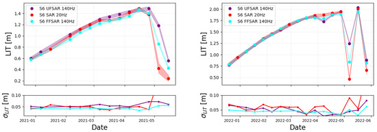
Figure 7.
Comparison of the LIT estimates obtained with Sentinel-6 high-resolution SAR data for one ice season at Great Slave Lake (left) and Baker Lake (right). The curves refer to UFSAR at 20 Hz (red), UFSAR at 140 Hz (purple), and FFSAR at 140 Hz (cyan).

Table 1.
Comparison of the LIT results from radar altimetry data and thermodynamic CLIMo simulations. The table summarizes the following indicators: the maximum LIT estimates, , with the corresponding date, the LIT mean, , the MBE and RMSE between the LIT estimates from Sentinel-6 UFSAR at 20 Hz and the other datasets (see details in the text of Section 5).
Overall, the results show a significant improvement in the precision of LIT estimates in comparison to previous analysis, in particular when using conventional altimetry data, thanks to the higher resolution of the Sentinel-6 SAR data.
5.2. Evaluation and Consistency
The evaluation of the SAR_LIT retracker analysis is performed by quantitatively comparing the Sentinel-6 UFSAR 20 Hz LIT estimates to those obtained from the thermodynamic simulations (CLIMo), described in Section 4.3, and to the LIT estimates derived from the LRM_LIT analysis [13] of low-resolution-mode (LRM) data of both Sentinel-6 and Jason-3 during their tandem phase. Assessing the consistency between the SAR and LRM estimates is particularly important to ensure the stability of the LIT measurements between current and future altimetry missions. The LIT indicators and metrics used for the comparison are, as summarized in Table 1 for both lake targets, the LIT maximum and the corresponding date, the mean LIT in the middle of the ice season when the ice is well established on the lakes (1st February to mid-April), with the associated uncertainty, the mean bias error (MBE), and the root mean square error (RMSE) between the Sentinel-6 UFSAR 20 Hz and the other datasets. It is worth noting here that in the Table 1 the LIT indicators are reported for the 2020–2021 season for Great Slave and for the 2021–2022 season for Baker due to a fair amount of missing waveform data in the other ice seasons (missing input data for cycles for Great Slave in the 2021–2022 season and missing input data for 10 cycles for Baker in the 2020–2021 season). As shown in Figure 8 and Figure 9, despite the missing data, the LIT evolution is consistently captured for both seasons and lakes, and the LIT indicators reported are, therefore, representative of a typical ice season.
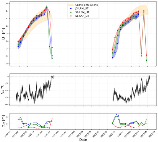
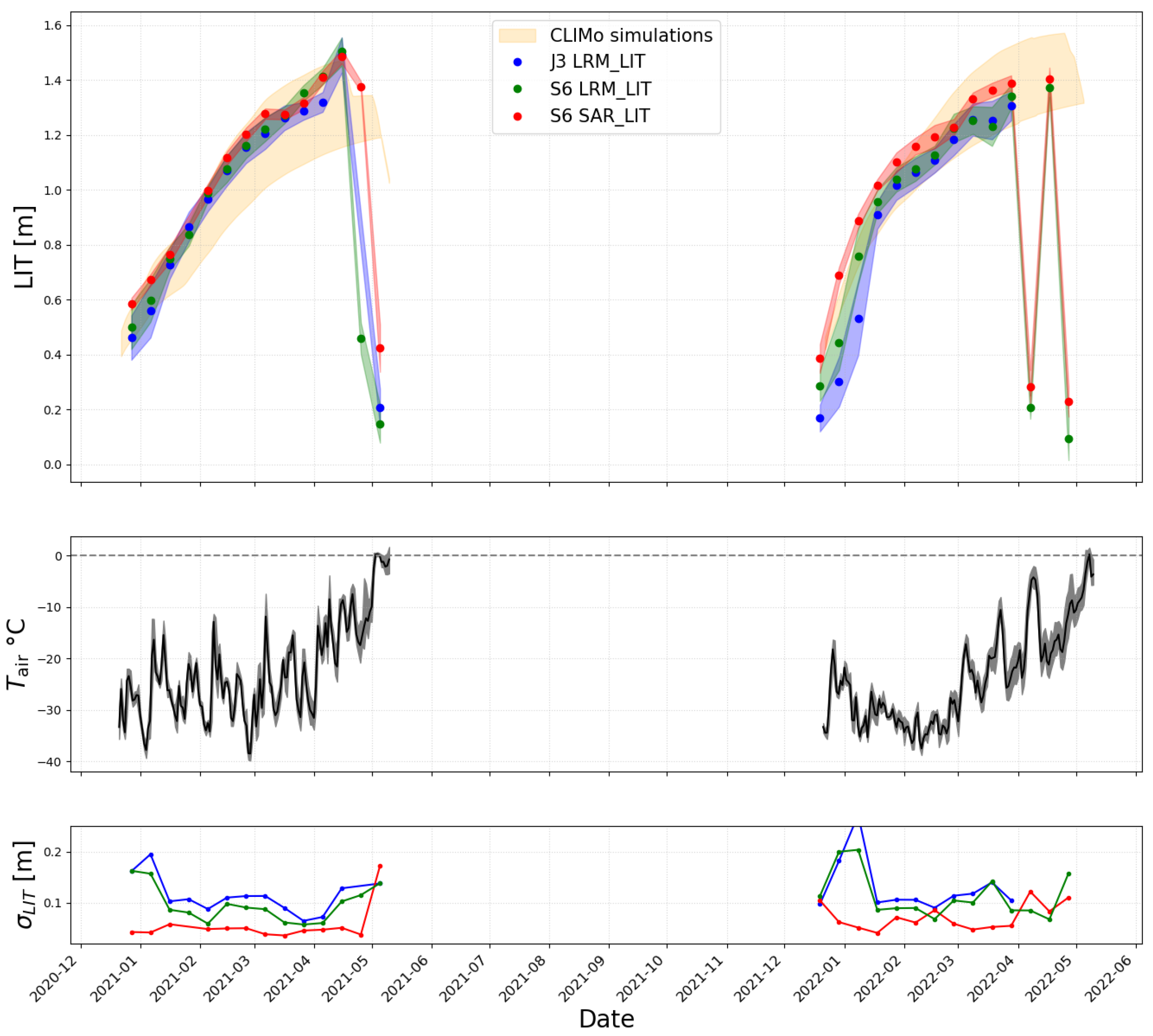
Figure 8.
Evolution of LIT estimates at Great Slave Lake obtained with Sentinel-6 UFSAR at 20 Hz data (red), Sentinel-6 LRM data (green) and Jason-3 data (blue) for the 2020–2021 and 2021–2022 ice seasons (upper panel). The shaded regions of the corresponding colors refer to the LIT error envelopes at 1 for each case. The orange shaded area shows the evolution of LIT obtained from CLIMo thermodynamic simulations with different on-ice snow scenarios (see text in Section 4.3 for details). The middle panel shows the evolution of the mean 2 m air temperature (black) with the minimum and maximum values (gray shading) extracted from ERA5 data. The bottom panel shows the evolution of the 1 LIT uncertainties for the three datasets.
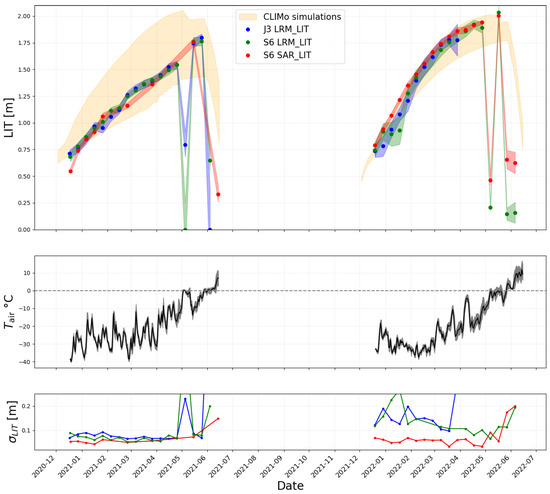
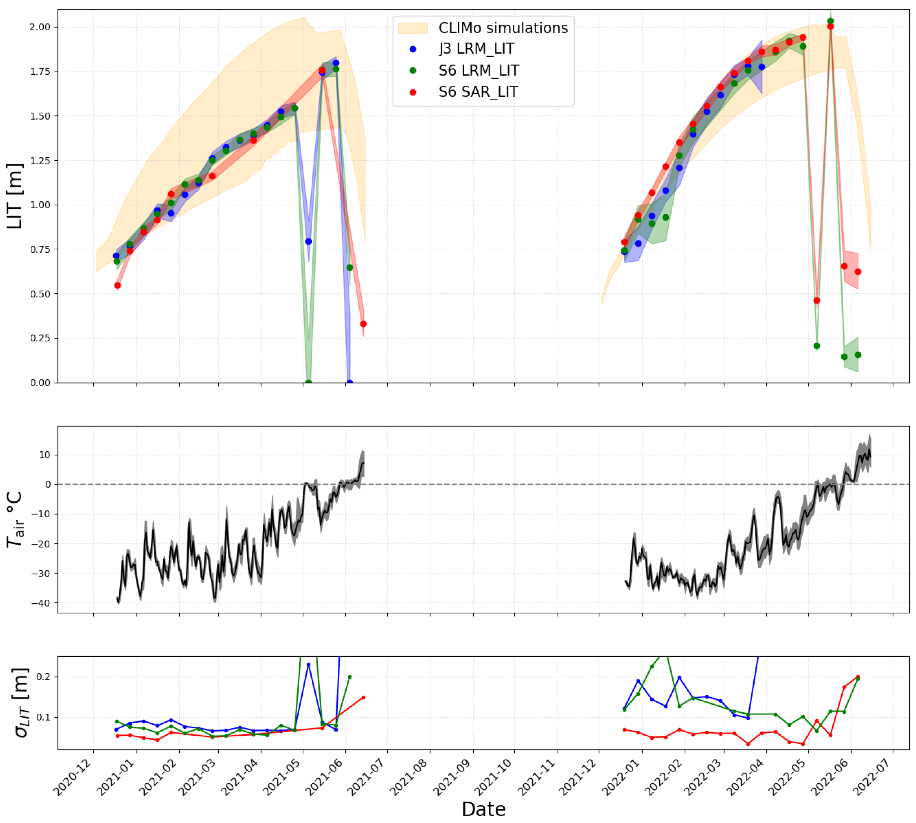
Figure 9.
Evolution of the LIT estimates at Baker Lake obtained with different datasets (see the caption of Figure 8 for details).
Figure 8 and Figure 9 summarize the comparison of LIT among the different datasets for Great Slave Lake and Baker Lake, respectively. In both figures, the top panel shows LIT estimates obtained with the Sentinel-6 UFSAR at 20 Hz data (red), the Sentinel-6 LRM data (green) and the Jason-3 data (blue) for the 2020–2021 and 2021–2022 ice seasons during the Sentinel-6 and Jason-3 tandem phase (December 2020–April 2022). The shaded regions of the corresponding colors refer to the LIT error envelopes at 1 for each case. The orange shaded area shows the evolution of LIT obtained with the CLIMo thermodynamic simulations with different snow-on-ice scenarios: the upper bound refers to the simulations without snow on the ice surface, while the lower bound to the simulations with 75% of snow with respect to snow depth measured at nearby meteorological stations on land (see Section 4.3 for details). The middle panel in both figures shows the evolution of the mean 2 m daily air temperature (black line) with the gray shaded area delineating the minimum and maximum daily temperatures extracted from ERA5 hourly data. Plotting air temperature measurements along with the LIT estimates is useful since it provides some information about the status of the lake surface, revealing snow-on-ice melt when the air temperature is near or greater than 0 °C, and refreeze when temperatures drop again below 0 °C during the spring transition period. Finally, the bottom panel highlights the evolution of the LIT standard deviation derived from the three datasets (same legend as in the top panel).
Overall, there is a very good consistency among the SAR and LRM LIT results. The MBE and RMSE of Sentinel-6 SAR and LRM LIT estimates are 1.7 cm and 3.3 cm, respectively, for Great Slave Lake and 2.3 cm and 3.2 cm, respectively, for Baker Lake. The agreement with Jason-3 is also very appreciable, with MBE and RMSE of 4 cm for Great Slave and 7 cm for Baker. The maximum LIT and the LIT mean are also estimated consistently within a few centimeters difference among the different datasets. The dates of maximum LIT are also fully consistent between the SAR and LRM. The LIT evolution is in agreement with the output of the CLIMo simulations, within the uncertainty envelope given by the different snow-on-ice scenarios used as input. For both lake targets and for the seasons considered for the quantitative analysis, the satellite-based LIT estimates seem to be more in agreement with a small amount of snow (25%) or no snow on ice in terms of LIT maximum (values and date) and mean, and with MBE and RMSE values that are the smallest for the simulations with no snow on the ice, being −7 cm and 8 cm, respectively, for Great Slave and −3 cm and 5 cm, respectively, for Baker Lake.
As shown in the figures, LIT drops are detected right before the maximum is reached, at the end of the ice season, during the 2021–2022 season for Great Slave and during both seasons for Baker Lake. These drops are expected and are similar to those observed in previous studies (e.g., [7,13]). It can happen in fact that the snow/ice on the lake surface starts to melt due to an increase in temperatures, as discussed above, in which case the LIT signature is no longer present in the radar waveforms, so no, or a very small, LIT is retrieved. Then, with refreezing, the LIT signature is again detectable. As shown in the middle panels of Figure 8 and Figure 9, a clear correlation can in fact be seen between the detected LIT drops and the rise in the air temperature near or above 0 °C, supporting this explanation. As pointed out in [13], it is worth reiterating here that radar altimetry LIT retrackers can indeed capture the seasonal transitions of ice forming and melting but cannot precisely follow the ice evolution at the transitions because of the difficulty in retracking heterogeneous surfaces when the ice is too thin (fall freeze-up period) and when the snow on the ice surface begins to melt (spring break-up period). For this reason, as can be seen in the figures, the satellite-based LIT estimates drop at the beginning of melt, thus earlier with respect to the thermodynamic CLIMo simulations, that realistically generate LIT estimates throughout the whole melt period.
It can be noted that the LIT evolution is different at Great Slave and Baker, which is expected since the lakes are located at different latitudes and have distinct characteristics, as indicated earlier. For instance, the LIT maximum measured with Sentinel-6 20 Hz UFSAR occurs on 15 April and is m at Great Slave Lake, while for Baker Lake it generally occurs roughly one month later, on 17 May, and is 50 cm greater, reaching m. Also, the mean LIT in the middle of the ice season (as measured from February to April) is lower at Great Slave ( m) compared to Baker ( m). These results show that the SAR_LIT retracker can precisely follow the LIT evolution on different target lakes.
As expected, and as shown in the bottom panel of Figure 8 and Figure 9, the LIT estimates obtained from SAR data, because of the improved spatial resolution, show a significantly smaller dispersion with respect to the LIT estimates obtained with LRM data, thus yielding an LIT uncertainty that is a factor of ~2, up to 3, times smaller, depending on the season and target, with respect to the LRM estimates. For instance, as detailed in Table 1, the uncertainty in the maximum LIT estimation during the 2020–2021 season at Great Slave Lake with Sentinel-6 SAR data is 2.5 cm, compared to 5.1 cm with Sentinel-6 LRM data and 6.4 cm with Jason-3 LRM data, thus a factor of 2 and 2.6 smaller, respectively.
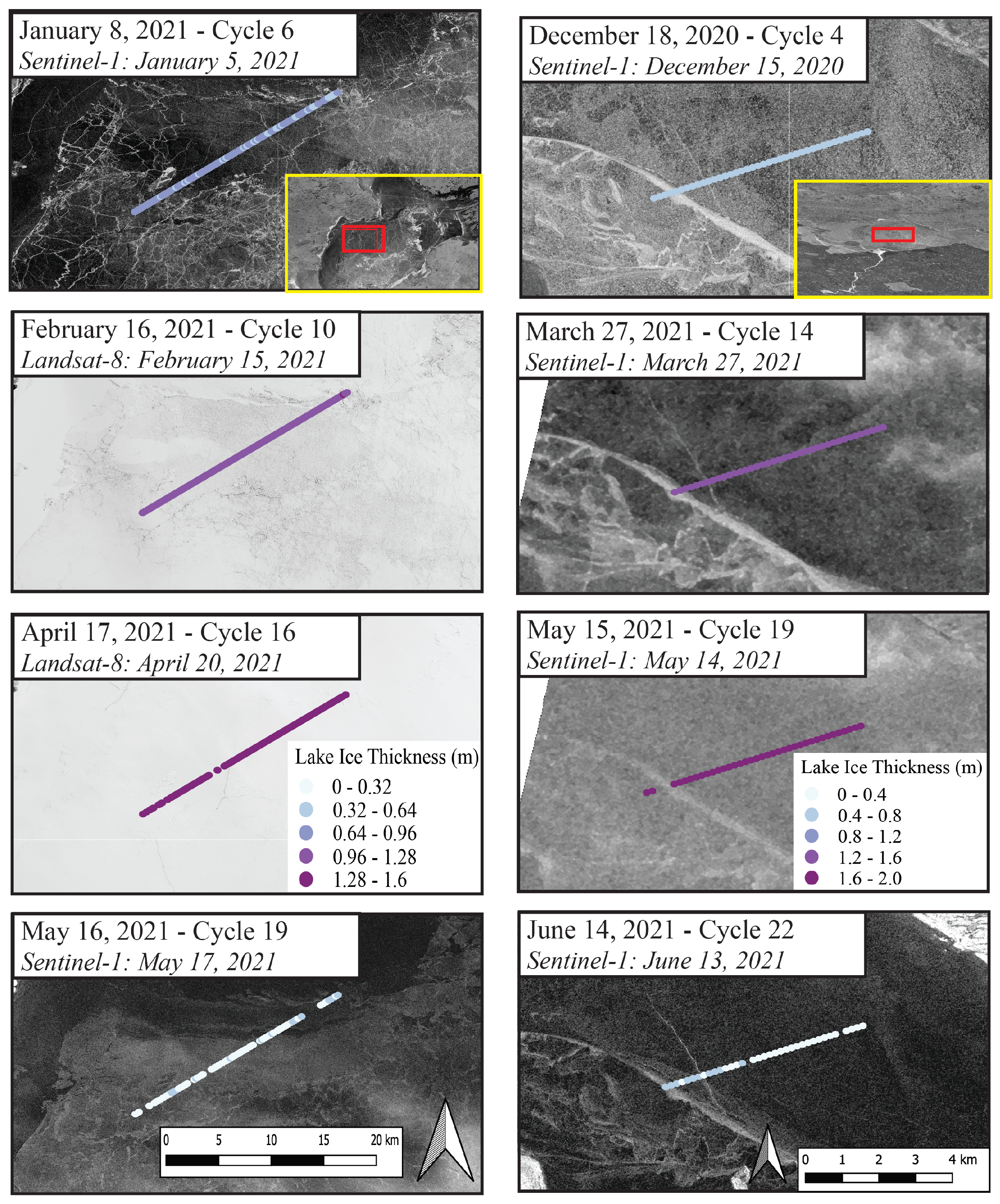
Finally, we performed consistency checks by superimposing the LIT estimates obtained with the SAR_LIT retracker applied to Sentinel-6 20 Hz UFSAR data onto optical (Landsat-8) or radar (Sentinel-1) images, according to the images availability on the Sentinel-6 flyover dates over the two lakes. This is illustrated in Figure 10 for Great Slave Lake (left) and Baker Lake (right), where the Sentinel-6 LIT estimates along the ROI track segment are overlaid on the images and color coded, ranging from 0 to 1.6 m for Great Slave and from 0 to 2 m for Baker. The images and LIT estimates are shown for representative dates following the typical duration of the ice season for the two lake targets, from January to May for the Great Slave lake and from December to June for the Baker lake. Overall, there is a very good consistency between the LIT estimates and the lake surface conditions for both target lakes, with thinner ice detection at the beginning of the ice season when the images show a heterogeneous surface of initial ice formation and open water (top panels), consistently growing LIT in the middle of the ice season when the snow/ice cover uniform over the lake surface (second and third panels), and drop in the LIT estimates to small values at the end of the season with snow melt, as shown in the bottom panels.
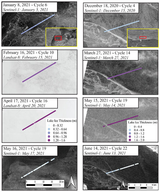
Figure 10.
Sentinel–6 20 Hz UFSAR LIT estimates superimposed on radar/optical images taken on the same dates for Great Slave Lake (left) and Baker Lake (right) on the lake area shown in the red boxes in the top row panels.
6. Conclusions and Outlook
In this paper, we presented a novel, efficient, analytically based retracking approach for the estimation of LIT from high-resolution Ku-band SAR (FFSAR and UFSAR) altimetry data. We carried out the LIT analysis with Sentinel-6 UFSAR data at 20 Hz and with UFSAR and FFSAR data at 140 Hz. We evaluated the SAR_LIT and FFSAR_LIT retracker analysis with LIT obtained from numerical lake ice model simulations and estimates from Sentinel-6 and Jason-3 conventional LRM altimetry data at 20 Hz for two ice seasons during the tandem phase of the two satellites. We performed consistency checks by superimposing the along-track Sentinel-6 LIT estimates on optical and radar images. We performed the LIT analysis and assessment for Great Slave Lake and Baker Lake (Canada), two lakes that differ in terms of their size, bathymetry, and snow/ice properties. The results demonstrate the ability of the SAR_LIT and FFSAR_LIT retrackers to retrieve robust LIT estimates over different ice seasons and for lakes of varied characteristics. The estimates are in high agreement with those obtained from LRM data, ensuring the continuity of LIT measurements and time series from conventional altimetry missions as well as current and future SAR altimetry missions. The typical LIT uncertainty obtained with the SAR_LIT retracker is of the order of 5 cm when the ice is well established on the lake, representing a significant improvement with respect to previous studies (as, e.g., [7,8,9,10,11]). As expected, the estimated LIT uncertainties are significantly smaller, by a factor of 2 to 3, when using Sentinel-6 UFSAR data at 20 Hz in contrast to LRM data due to increased resolution. The FFSAR processing at 140 Hz provides even better LIT estimates with 20% smaller uncertainties. The LIT retracker analysis performed on data at the higher posting rate (140 Hz) shows increased performance in comparison to the 20 Hz data, especially during the melt transition period, due to the increased statistics (a factor of seven times more data points, and therefore, a higher spatial sampling of the lake surface).
As previously reported by [13], the main limitation of LIT retrackers based on Ku-band waveform data is that they work well if the ice-related signature, that is, the double-peak feature in the Ku-band radar waveforms, is present. Indeed, the freshwater ice signature depends on the properties and thickness of the snowpack and the ice cover. The double-peak feature in the waveform may be absent if some conditions are not met, for instance, in the case of melting snow on the ice surface or snow-free lake ice. For this reason, the SAR_LIT and FFSAR_LIT retrackers can capture snow/ice melt onset on a lake, but they cannot precisely follow the evolution of LIT during melt periods since the radar waves are reflected by the surface (i.e., they do not penetrate through wet snow and ice). Also, there may be lakes for which the ice signature is not clearly visible or not present, as is the case for snow-free areas on lakes. In such a situation, consistent LIT estimates and time series cannot be generated for these lake targets. Overall, as long as the LIT signature is present in the radar waveforms, the SAR_LIT and FFSAR_LIT retrackers can precisely capture the seasonal evolution and the inter-annual variability in LIT, making them powerful tools for obtaining robust LIT estimates required for climate monitoring.
This research has identified several topics that merit further investigation. First, Ku-band SAR LIT time series should be generated for different lake targets and from different SAR altimetry missions, for instance, Sentinel-6, Cryosat-2, and Sentinel-3, enriching the LIT time series datasets currently being generated within the ESA Lakes_cci project, which consists of LIT long time series generated from LRM data (the LIT product over one target, the Great Slave lake, has been publicly released at the end of 2023, LIT products for more lakes will be released in 2025). Sentinel-3 is of particular interest since it allows for the inclusion of lakes located at latitudes higher (above 66 deg N) than is possible from Jason/Sentinel-6 altimetry missions, enabling a broader spatial coverage of LIT monitoring. Another key topic is understanding the propagation of radar waves through snow and ice of various properties at different frequencies (e.g., Ka and Ku-band).
Radiative transfer modeling experiments on the impact of ice and overlying snow properties on altimeter waveforms (Ka/Ku-band) at several lake sites are needed in parallel, building on the recent ESA LIAM project [29] that established a modeling framework that integrates the Snow Microwave Radiative Transfer (SMRT) model and the lake ice model CLIMo with simulations that can currently be performed in LRM, but that should be extended to SAR mode. A multi-sensor/frequency approach is also needed to assess the possibility of retrieving on-ice snow depth. This topic is particularly relevant in view of the future Copernicus Polar Ice and Snow Topography Altimeter (CRISTAL) mission (https://www.eoportal.org/satellite-missions/cristal-copernicus-polar-ice-and-snow-topography-altimeter-#overview, accessed on 28 June 2024), planned for launch in 2027, that will carry a dual-frequency Ku/Ka-band radar altimeter [30]. In the case of freshwater lake ice covered by dry snow, Ka and Ku-band radar waves may be reflected at the air/snow (or at other interfaces within the snowpack) and snow/ice interfaces, and the snow/ice and ice/water interfaces, respectively. However, the propagation of the radar waves at different frequencies depends on the properties of ice and overlying snow properties (e.g., ice type, snow density, and surface roughness) and is not fully understood yet. Field campaigns offer an opportunity to improve characterization of the Ka/Ku-bands through monitoring of ice/snow properties. This can be useful for parameterizing radiative transfer models to better understand the impact of these properties on radar waveforms from ice cover. Additionally, future work should investigate the impact of changing ice roughness on the retrieval by retrackers. The roughness of interfaces within the ice and snow column has been an area of interest in recent years and further investigation could provide better insights into the impact of these properties on radar waves and could be further supported by radiative transfer models such as SMRT. The lakes could be considered as cal/val sites for regular monitoring and assessing the performance of the dual-band measurements of the CRISTAL upcoming mission. A SAR_LIT retracker, based on the work presented in this paper and tailored for the CRISTAL mission, is currently being developed and validated within the ESA CLE2VER project and will be implemented in the CRISTAL prototype processor.
Author Contributions
Conceptualization, A.M.; methodology, A.M.; software, A.M., C.R.D., J.M., T.M., S.A. and J.S.M.; validation, A.M., C.R.D., J.M. and J.S.M.; formal analysis, A.M., investigation, A.M., C.R.D., J.M., J.S.M., T.M., S.A. and P.T.; data curation, A.M., C.R.D., J.M., T.M. and S.A.; writing—original draft preparation, A.M.; writing—review and editing, A.M., C.R.D., J.M. and T.M.; funding acquisition, C.D. All authors have read and agreed to the published version of the manuscript.
Funding
This research was funded by the European Space Agency (ESA), under ESA Contract No. 4000134346/21/NL/AD.
Data Availability Statement
The data supporting the findings of this study are publicly available and can be downloaded from the EUMETSAT Data Centre at https://user.eumetsat.int/data-access/data-centre, accessed on 28 June 2024.
Conflicts of Interest
Authors Claude R. Duguay, Justin Murfitt and Jaya Sree Mugunthan were employed by the company H2O Geomatics, Author Samira Amraoui was employed by the company Bioceanor. The remaining authors declare that the research was conducted in the absence of any commercial or financial relationships that could be construed as a potential conflict of interest.
Appendix A. Sentinel-6 System and Sensor Parameters
The Sentinel-6 system and sensor parameters used in the SAR_LIT and the FFSAR_LIT waveform models are summarized in Table A1.
Table A1.
System and sensor parameters for Sentinel-6.
Table A1.
System and sensor parameters for Sentinel-6.
| Symbol | Description | Value |
|---|---|---|
| Central frequency | 13.575 GHz | |
| PTR time width | 0.8846 | |
| h | Nominal orbit height | 1347 km |
| Nominal satellite velocity | 6965 m/s | |
| Number of pulses per burst | 64 | |
| Pulse repetition frequency | 9175 Hz | |
| Half-power along track beam width | 1.33 deg | |
| Half-power across track beam width | 1.33 deg | |
| L | Total number of Doppler beams | 448 |
| B | Bandwidth | 320 MHz |
| Sampling frequency | 395 MHz |
References
- World Meteorological Organization. The 2022 GCOS ECVs Requirements (GCOS-245); World Meteorological Organization: Geneva, Switzerland, 2022; 244p. [Google Scholar]
- Ghiasi, Y.; Duguay, C.; Murfitt, J.; van der Sanden, J.; Thompson, A.; Drouin, H.; Prévost, C. Application of GNSS interferometric reflectometry for the estimation of lake ice thickness. Remote Sens. 2020, 12, 2721. [Google Scholar] [CrossRef]
- Brown, L.C.; Duguay, C.R. The fate of lake ice in the North American Arctic. Cryosphere Discuss. 2011, 5, 1775–1834. [Google Scholar] [CrossRef]
- Murfitt, J.; Duguay, C.R. 50 years of lake ice research from active microwave remote sensing: Progress and prospects. Remote Sens. Environ. 2021, 264, 112616. [Google Scholar] [CrossRef]
- Kang, K.K.; Duguay, C.R.; Howell, S.E.L.; Derksen, C.; Kelly, R. Sensitivity of AMSR-E brightness temperatures to the seasonal evolution of lake ice thickness. IEEE Geosci. Remote Sens. Lett. 2010, 7, 751–755. [Google Scholar] [CrossRef]
- Kang, K.K.; Duguay, C.; Lemmetyinen, J.; Gel, Y. Estimation of ice thickness on large northern lakes from AMSR-E brightness temperature measurements. Remote Sens. Environ. 2014, 150, 1–19. [Google Scholar] [CrossRef]
- Beckers, J.F.; Alec Casey, J.; Haas, C. Retrievals of lake ice thickness from Great Slave Lake and Great Bear Lake using CryoSat-2. IEEE Trans. Geosci. Remote Sens. 2017, 55, 3708–3720. [Google Scholar] [CrossRef]
- Ye, H.; Jin, G.; Zhang, H.; Xiong, X.; Li, J.; Wang, J. Lake ice thickness retrieval method with ICESat-2-assisted CyroSat-2 echo peak selection. Remote Sens. 2024, 16, 546. [Google Scholar] [CrossRef]
- Shu, S.; Liu, H.; Beck, R.A.; Frappart, F.; Korhonen, J.; Xu, M.; Yang, B.; Hinkel, K.M.; Huang, Y.; Yu, B. Analysis of Sentinel-3 SAR altimetry waveform retracking algorithms for deriving temporally consistent water levels over ice-covered lakes. Remote Sens. Environ. 2020, 239, 111643. [Google Scholar] [CrossRef]
- Yang, Y.; Moore, P.; Li, Z.; Li, F. Lake level change from satellite altimetry over seasonally ice-covered lakes in the Mackenzie River Basin. IEEE Trans. Geosci. Remote Sens. 2021, 59, 8143–8152. [Google Scholar] [CrossRef]
- Li, X.; Long, D.; Huang, Q.; Zhao, F. The state and fate of lake ice thickness in the Northern Hemisphere. Sci. Bull. 2022, 67, 537–546. [Google Scholar] [CrossRef]
- Li, X.; Long, D.; Cui, Y.; Liu, T.; Lu, J.; Hamouda, M.A.; Mohamed, M.M. Ice thickness and water level estimation for ice-covered lakes with satellite altimetry waveforms and backscattering coefficients. Cryosphere 2023, 17, 349–369. [Google Scholar] [CrossRef]
- Mangilli, A.; Thibaut, P.; Duguay, C.R.; Murfitt, J. A New approach for the estimation of lake ice thickness from conventional radar altimetry. IEEE Trans. Geosci. Remote Sens. 2022, 60, 4305515. [Google Scholar] [CrossRef]
- Raney, R. The delay/Doppler radar altimeter. IEEE Trans. Geosci. Remote Sens. 1998, 36, 1578–1588. [Google Scholar] [CrossRef]
- Egido, A.; Smith, W.H.F. Fully focused SAR altimetry: Theory and applications. IEEE Trans. Geosci. Remote Sens. 2017, 55, 392–406. [Google Scholar] [CrossRef]
- Duguay, C.; Flato, G.; Jeffries, M.; Menard, P.; Morris, K.; Rouse, W. Ice cover variability on shallow lakes at high latitudes: Model simulations and observations. Hydrol. Process. 2003, 17, 3465–3483. [Google Scholar] [CrossRef]
- Gunn, G.; Duguay, C.; Brown, L.; King, J.; Atwood, D.; Kasurak, A. Freshwater lake ice thickness derived using surface-based X- and Ku-band FMCW scatterometers. Cold Reg. Sci. Technol. 2015, 120, 115–126. [Google Scholar] [CrossRef]
- Ray, C.; Martin-Puig, C.; Clarizia, M.P.; Ruffini, G.; Dinardo, S.; Gommenginger, C.; Benveniste, J. SAR altimeter backscattered waveform model. IEEE Trans. Geosci. Remote Sens. 2015, 53, 911–919. [Google Scholar] [CrossRef]
- Dinardo, S. Techniques and Applications for Satellite SAR Altimetry over Water, Land and Ice. Ph.D. Thesis, Technische Universität, Darmstadt, Germany, 2020. [Google Scholar] [CrossRef]
- Donlon, C.; Cullen, R.; Giulicchi, L.; Fornari, M.; Vuilleumier, P. Copernicus Sentinel-6 Michael Freilich satellite mission: Overview and preliminary in orbit results. In Proceedings of the 2021 IEEE International Geoscience and Remote Sensing Symposium IGARSS, Brussels, Belgium, 11–16 July 2021; pp. 7732–7735. [Google Scholar] [CrossRef]
- Ehlers, F.; Schlembach, F.; Kleinherenbrink, M.; Slobbe, C. Validity assessment of SAMOSA retracking for fully-focused SAR altimeter waveforms. Adv. Space Res. 2023, 71, 1377–1396. [Google Scholar] [CrossRef]
- Ménard, P.; Duguay, C.R.; Flato, G.M.; Rouse, W.R. Simulation of ice phenology on Great Slave Lake, Northwest Territories, Canada. Hydrol. Process. 2002, 16, 3691–3706. [Google Scholar] [CrossRef]
- Rieu, P.; Amraoui, S.; Restano, M. SMAP (Standalone Multimission Altimetry Processor). 2021. Available online: https://github.com/cls-obsnadir-dev/SMAP-FFSAR (accessed on 24 June 2024).
- Murfitt, J.; Duguay, C.; Picard, G.; Gunn, G. Forward modelling of synthetic aperture radar backscatter from lake ice over Canadian Subarctic Lakes. Remote Sens. Environ. 2023, 286, 113424. [Google Scholar] [CrossRef]
- Surdu, C.M.; Duguay, C.R.; Brown, L.C.; Fernández Prieto, D. Response of ice cover on shallow lakes of the North Slope of Alaska to contemporary climate conditions (1950–2011): Radar remote-sensing and numerical modeling data analysis. Cryosphere 2014, 8, 167–180. [Google Scholar] [CrossRef]
- Kheyrollah Pour, H.; Duguay, C.R.; Scott, K.A.; Kang, K.K. Improvement of lake ice thickness retrieval from MODIS satellite data using a thermodynamic model. IEEE Trans. Geosci. Remote Sens. 2017, 55, 5956–5965. [Google Scholar] [CrossRef]
- Antonova, S.; Duguay, C.R.; Kääb, A.; Heim, B.; Langer, M.; Westermann, S.; Boike, J. Monitoring bedfast ice and ice phenology in lakes of the Lena River Delta using TerraSAR-X backscatter and coherence time series. Remote Sens. 2016, 8, 903. [Google Scholar] [CrossRef]
- Egido, A.; Dinardo, S.; Ray, C. The case for increasing the posting rate in delay/Doppler altimeters. Adv. Space Res. 2021, 68, 930–936. [Google Scholar] [CrossRef]
- Murfitt, J.; Duguay, C.R.; Picard, G.; Gunn, G.E. Investigating the effect of lake ice properties on multifrequency backscatter using the Snow Microwave Radiative Transfer Model. IEEE Trans. Geosci. Remote Sens. 2022, 60, 4305623. [Google Scholar] [CrossRef]
- Kern, M.; Cullen, R.; Berruti, B.; Bouffard, J.; Casal, T.; Drinkwater, M.R.; Gabriele, A.; Lecuyot, A.; Ludwig, M.; Midthassel, R.; et al. The Copernicus Polar Ice and Snow Topography Altimeter (CRISTAL) high-priority candidate mission. Cryosphere 2020, 14, 2235–2251. [Google Scholar] [CrossRef]


Disclaimer/Publisher’s Note: The statements, opinions and data contained in all publications are solely those of the individual author(s) and contributor(s) and not of MDPI and/or the editor(s). MDPI and/or the editor(s) disclaim responsibility for any injury to people or property resulting from any ideas, methods, instructions or products referred to in the content. |
© 2024 by the authors. Licensee MDPI, Basel, Switzerland. This article is an open access article distributed under the terms and conditions of the Creative Commons Attribution (CC BY) license (https://creativecommons.org/licenses/by/4.0/).