
Comment on Yu et al. Land Surface Temperature Retrieval from Landsat 8 TIRS—Comparison between Radiative Transfer Equation-Based Method, Split Window Algorithm and Single Channel Method. Remote Sens. 2014, 6, 9829–9852


Abstract
:1. Introduction
2. Comments about the Results and Correction
- K1_CONSTANT_BAND_10 = 774.8853 (W·m−2·μm−1)
- K2_CONSTANT_BAND_10 = 1321.0789 (K)
- K1_CONSTANT_BAND_11 = 480.8883 (W·m−2·μm−1)
- K2_CONSTANT_BAND_11 = 1201.1442 (K)
- is the thermal radiance measured at the top of the atmosphere;
- is the atmospheric transmittance for specific wavelengths;
- is the surface emissivity at specific wavelengths;
- are the downwelling and upwelling radiance, respectively, at specific wavelengths (the contribution of the atmosphere);
- is the thermal radiance at the Earth’s surface.
3. Conclusions
Author Contributions
Funding
Data Availability Statement
Acknowledgments
Conflicts of Interest
References
- Yu, X.; Guo, X.; Wu, Z. Land Surface Temperature Retrieval from Landsat 8 TIRS—Comparison between Radiative Transfer Equation-Based Method, Split Window Algorithm and Single Channel Method. Remote Sens. 2014, 6, 9829–9852. [Google Scholar] [CrossRef]
- United States Geological Survey (USGS). Available online: https://www.usgs.gov/landsat-missions/using-usgs-landsat-level-1-data-product (accessed on 5 January 2023).
- MAO, K.; Qin, Z.; Shi, J.; Gong, P. The research of split-window algorithm on the MODIS. Geomat. Inf. Sci. Wuhan Univ. 2005, 30, 703–707. [Google Scholar]
- Spectral Characteristics Viewer. Available online: https://landsat.usgs.gov/spectral-characteristics-viewer (accessed on 15 June 2023).
- Jiménez-Muñoz, J.C.; Sobrino, J.A. A Generalized Single-Channel Method for Retrieving Land Surface Temperature from Remote Sensing Data. J. Geophys. Res. Atmos. 2003, 109, 8112. [Google Scholar] [CrossRef]
- Qin, Z.; Karnieli, A.; Berliner, P. A mono-window algorithm for retrieving land surface temperature from Landsat TM data and its application to the Israel-Egypt border region. Int. J. Remote Sens. 2001, 22, 3719–3746. [Google Scholar] [CrossRef]


| Bands | (μm) |
|---|---|
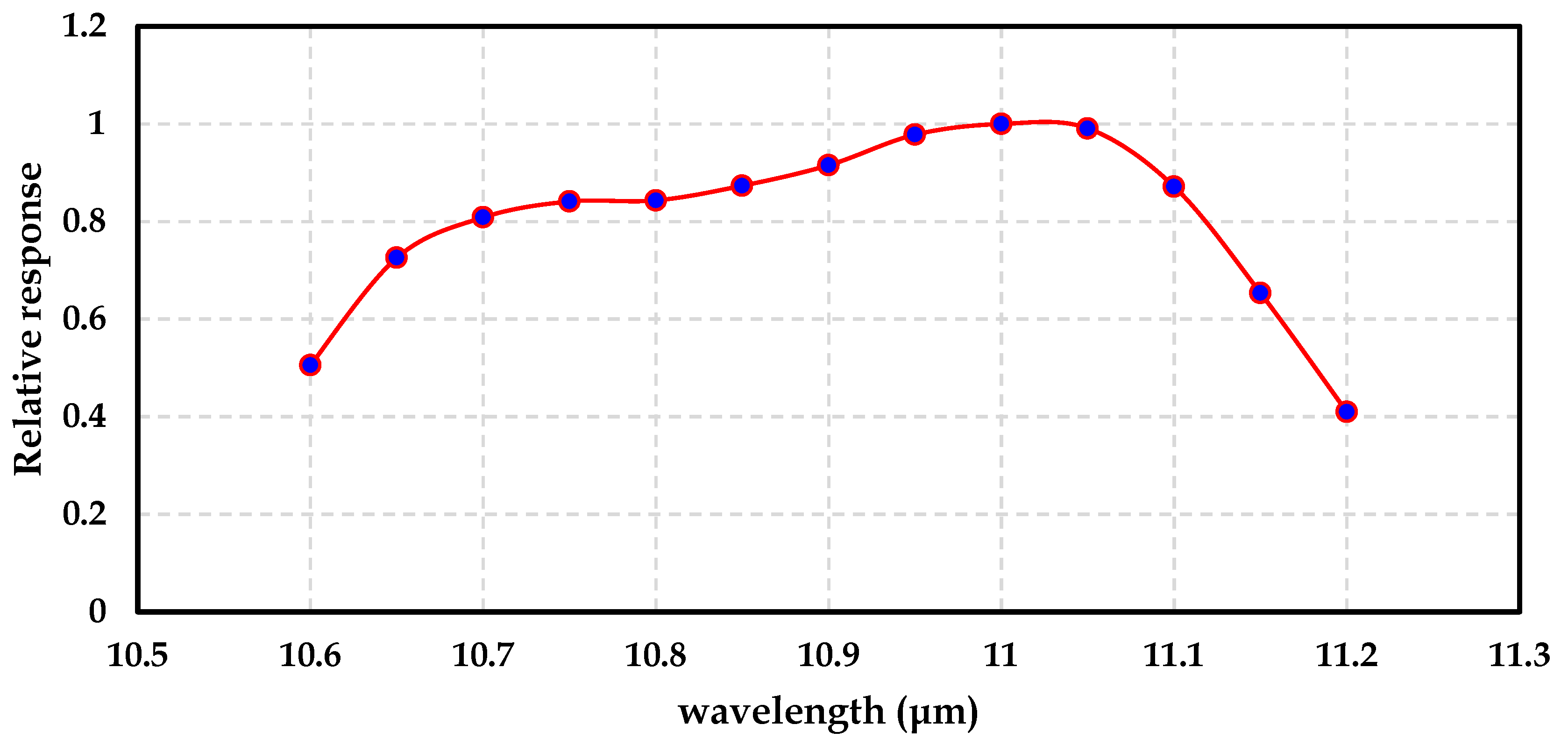
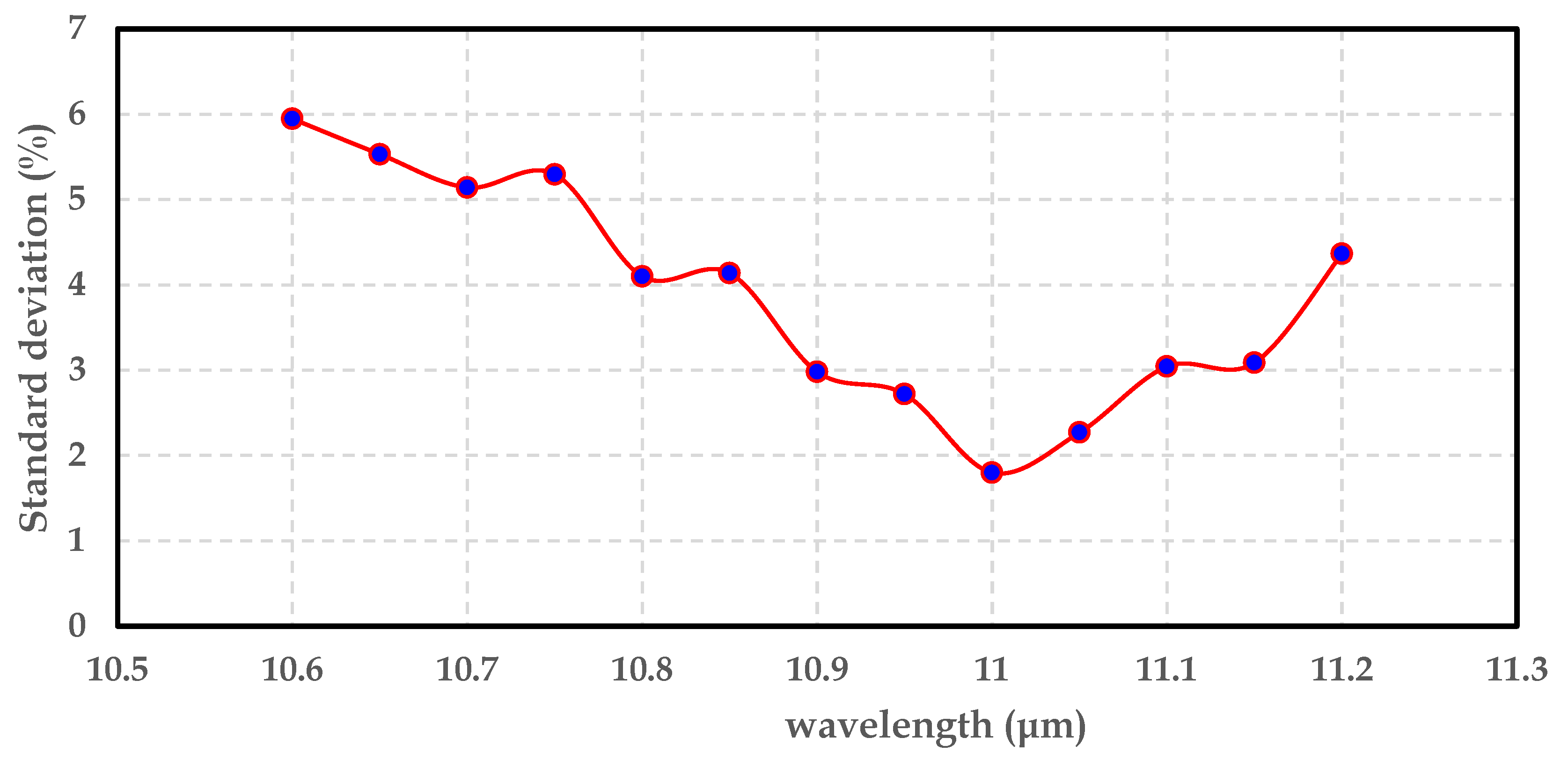
| L8 (Band 10) | 10.8909 |
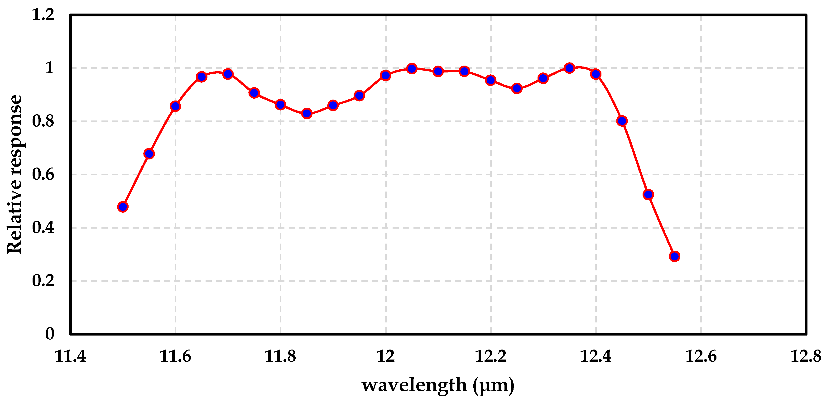
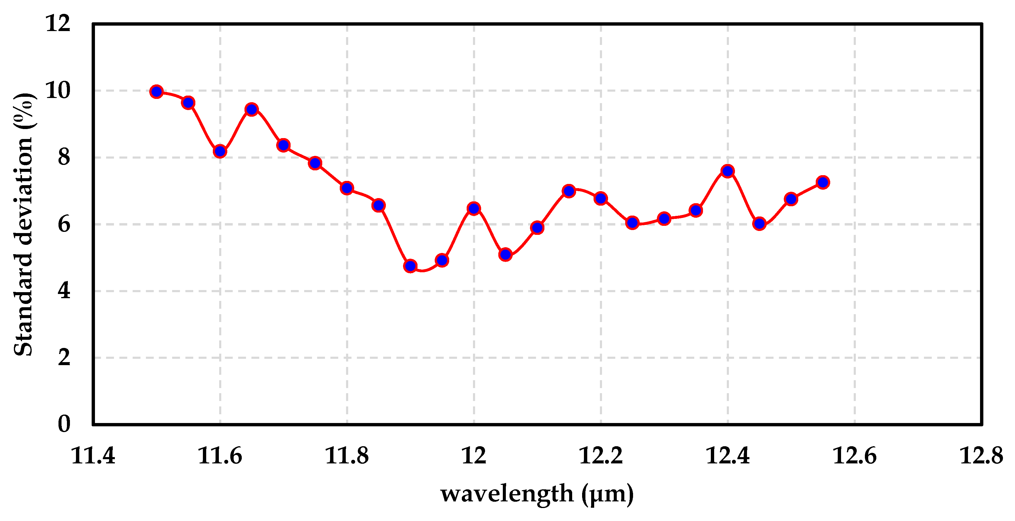
| L8 (Band 11) | 11.9784 |
| Bands | (μm) |
|---|---|
| L8 (Band 10) | 10.8977 |
| L8 (Band 11) | 11.9888 |
| Band | μm |
|---|---|
| L8 (Band 10) | 10.814 |
| L8 (Band 11) | 12.013 |
| Parameters | Spectral Functions |
|---|---|
| 0.00090 − 0.01638 + 0.04745 + 0.27436 | |
| 0.00032 − 0.06148 + 1.2021 − 6.2051 | |
| 0.00986 − 0.23672 + 1.7133 − 3.2199 | |
| −0.15431 + 5.2757 − 60.1170 + 229.3139 | |
| −0.02883 + 0.87181 − 8.82712 + 29.9092 | |
| 0.13515 − 4.1171 + 41.8295 − 142.2782 | |
| −0.22765 + 6.8606 − 69.2577 − 233.0722 | |
| 0.41868 − 14.3299 + 163.6681 − 623.53 | |
| 0.00182 − 0.04519 + 0.32652 − 0.60030 | |
| −0.00744 + 0.11431 + 0.17560 − 5.4588 | |
| −0.00269 + 0.31395 − 5.5916 + 27.9913 | |
| −0.07972 + 2.8396 − 33.6843 + 132.9798 |
Disclaimer/Publisher’s Note: The statements, opinions and data contained in all publications are solely those of the individual author(s) and contributor(s) and not of MDPI and/or the editor(s). MDPI and/or the editor(s) disclaim responsibility for any injury to people or property resulting from any ideas, methods, instructions or products referred to in the content. |
© 2024 by the authors. Licensee MDPI, Basel, Switzerland. This article is an open access article distributed under the terms and conditions of the Creative Commons Attribution (CC BY) license (https://creativecommons.org/licenses/by/4.0/).
Share and Cite
Ayek, A.A.E.; Zerouali, B. Comment on Yu et al. Land Surface Temperature Retrieval from Landsat 8 TIRS—Comparison between Radiative Transfer Equation-Based Method, Split Window Algorithm and Single Channel Method. Remote Sens. 2014, 6, 9829–9852. Remote Sens. 2024, 16, 2514. https://doi.org/10.3390/rs16142514
Ayek AAE, Zerouali B. Comment on Yu et al. Land Surface Temperature Retrieval from Landsat 8 TIRS—Comparison between Radiative Transfer Equation-Based Method, Split Window Algorithm and Single Channel Method. Remote Sens. 2014, 6, 9829–9852. Remote Sensing. 2024; 16(14):2514. https://doi.org/10.3390/rs16142514
Chicago/Turabian StyleAyek, Almustafa Abd Elkader, and Bilel Zerouali. 2024. "Comment on Yu et al. Land Surface Temperature Retrieval from Landsat 8 TIRS—Comparison between Radiative Transfer Equation-Based Method, Split Window Algorithm and Single Channel Method. Remote Sens. 2014, 6, 9829–9852" Remote Sensing 16, no. 14: 2514. https://doi.org/10.3390/rs16142514