Research on Inter-Satellite Laser Ranging Scale Factor Estimation Methods for Next-Generation Gravity Satellites

Abstract

The scale factor serves as a ruler for converting raw phase measurements into physical displacements and significantly impacts the preprocessing of data from the Laser Ranging Interferometer (LRI) in laser ranging systems. In the current GRACE Follow-On (GRACE-FO) mission for low–low tracking gravity satellites, most of the existing LRI scale factor estimation algorithms heavily rely on cross-calibration between instantaneous/biased ranges from the Ka-Band Ranging Interferometer (KBR) and the LRI. However, due to the nonlinearity of the objective function (which includes terms involving the product of scale and time shifts), the scale factor estimation may absorb errors from timing noise. Moreover, future gravity missions or gravity detection tasks may no longer incorporate KBR ranging instruments. To address these challenges, this paper proposes an energy-based method for scale factor estimation using inter-satellite baseline solutions. Comparative analysis indicates that the proposed method effectively disentangles two parameters in the objective function and can be applied in scenarios where KBR data are unavailable, demonstrating promising prospects for practical application. The experimental results show that when the KBR validation residuals are lower than 0.8 mm, the SYSU LRI1B V01 products exhibit residuals below the payload design accuracy thresholds in the frequency band of 2 mHz to 0.1 Hz. Additionally, the stability of the scale factors obtained from the baseline can reach 10⁻⁷. Although this is still below the required precision of better than 10⁻⁸ for the laser frequency stability in next-generation gravity satellites, advancements in orbit determination technology and the enhanced stability of GPS receivers offer potential for future precision improvements. Currently, this method appears suitable for roughly extracting the scale factor as a stochastic mean over several months or serving as a backup validation strategy for future missions, but it is not well suited to measure day-to-day variations.

1. Introduction

The GRACE-FO satellites, successfully launched by the United States and Germany in May 2018 at the California launch site, orbit at an average altitude of 491.5 km, with an inter-satellite distance of 216.7 km [1]. Over the past six years, they have accumulated a substantial amount of observational data on the Earth’s gravity field. In addition to the MWI carried by their predecessor, the GRACE satellites, GRACE-FOs are equipped with the LRI for the first time. This new instrument demonstrates the next generation of inter-satellite ranging technology [2]. Both the microwave instrument and the LRI provide highly precise measurements of distance changes. Through these differential measurements, the high-frequency content of the Earth’s gravitational signal is amplified, significantly enhancing the estimation of higher-resolution features of the Earth’s gravity field. Current on-orbit results from GRACE-FO demonstrate that the LRI can provide ranging data with an accuracy two or three orders of magnitude better than that of the KBR, with a ranging precision of up to 10 nanometers, thus holding significant potential for obtaining high-precision Earth gravity fields and advancing satellite gravity technology for scientific applications [3]. As a technological demonstrator, the LRI has successfully demonstrated the feasibility of inter-satellite laser interferometry in future geodetic missions. To further improve the observation accuracy and spatial–temporal resolution of the Earth’s gravity field and enhance its scientific value, China, Europe, the United States, and other countries are all actively promoting next-generation gravity satellite programs. Examples include the NGGM gravity satellite program [4] and the TianQin2 experimental satellite [5]. In the next generation of gravity missions, the laser interferometer is expected to replace the MWI as the primary scientific instrument [6].

The preprocessing techniques for LRI data encompass several critical steps, including phase unwrapping, time correction, phase jump handling, scale factor estimation, and light time correction [7]. Effective handling of these steps significantly enhances the practicality of LRI data and holds paramount importance in the initial data processing stages of scientific experiments [8]. Among these steps, phase jump handling and scale factor correction still present technical challenges. Phase jump handling techniques are discussed in detail in [9,10,11], while this paper primarily focuses on scale factor estimation research.

The formula ($\rho =c/\nu \cdot \phi$) can be used to calculate the inter-satellite distance. However, the laser frequency can experience fluctuations and drift over time due to thermal noise and stress variations in the frequency stabilization cavity, which cannot be directly measured in orbit [10]. Currently, the accuracy of distance measurements is improved by correcting the laser frequency through estimating the LRI scale factor. There are several main methods for estimating the scale factor, including the following: (1) cross-calibration estimation: This method utilizes cross-calibration between the KBR and LRI ranges to obtain the LRI scale factor [8,11]; (2) the exponential model method: The AEI utilizes the cross-calibration estimation method to generate daily scale factor values over multiple years and fits an exponential model by analyzing the characteristics of historical scale factors [12]; (3) a telemetry-based laser frequency model: This method is less dependent on the KBR instrument, which may be used in the future geodesy missions [9,12]; (4) absolute frequency readouts derived from the ULE cavity method: This method is independent of the KBR instrument, but it requires the installation of SFU hardware on board, which introduces minimal additional parts to the flight heritage GRACE-FO LRI baseline design [13]; (5) the joint gravity field estimation method: The AEI proposes a conceptual approach to determining the frequency from in-flight telemetry, which is to co-estimate it during gravity field recovery, as this is usually applied to the accelerometer scales and biases [12,14]. Among these methods, the cross-calibration estimation method is the most mature.

Due to the nonlinearity between the scale factor and time shift (this daily estimated time offset seeks to capture any unknown bias between the LRI and Receiver Time outside of the known data bias and filter delays [8]) in the objective function of cross-calibration, the scale factor estimation may absorb the errors from timing noise. Moreover, future gravity missions or gravity detection tasks may no longer incorporate KBR ranging instruments. To address these two issues, this paper proposes a frequency domain scale factor estimation method using inter-satellite baseline solutions. This method separates the estimation of the scale factor and time shift by determining the scale factor in the frequency domain. Subsequently, after applying the scale factor, the time shift is estimated by solving linear equations. The new method is applied to the comparison of GPS-derived baseline estimates with LRI data due to the non-existence of the KBR in future gravity missions. In most cases, the residuals between the SYSU LRI1B V01 product generated using this method and AEI V50 are below the payload design accuracy thresholds within the LRI’s design noise frequency band of 2 mHz to 0.1 Hz, satisfying the precision requirements for gravity field inversion.

2. Current Methods

Since this study involves data analysis for the LRI using publicly available data, we will focus on discussing cross-calibration here. Both JPL and AEI V50 utilize the criterion of the minimum RMSE based on the distances between the LRI and KBR for cross-calibration to obtain the scale factor and time shift. However, they differ in their approaches: JPL employs least squares cross-calibration using instantaneous ranges from JPL LRI and JPL KBR1B, while the AEI uses biased ranges from AEI LRI and JPL KBR1B for cross-calibration. The two methods will be illustrated in detail as follows.

2.1. Cross-Calibration by JPL

In JPL, a daily multiplicative scale correction of the range quantity and its time derivatives is estimated via least-squares estimation that seeks to minimize the difference between the LRI and KBR instantaneous, i.e., corrected, ranges, that is

$$\min \left|\right|{\rho }_{\mathrm{LRI}\text{\_}\mathrm{inst}}(t+\Delta t)\cdot s-{\rho }_{\mathrm{KBR}\text{\_}\mathrm{inst}}(t)\left|\right|$$

(1)

Since Δt is very small, we can expand it using Taylor series to obtain

$$\cong \min \left|\right|s\cdot {\rho }_{\mathrm{LRI}\text{\_}\mathrm{inst}}(t)+s\cdot \Delta t\cdot {\dot{\rho }}_{\mathrm{LRI}\text{\_}\mathrm{inst}}(t)-{\rho }_{\mathrm{KBR}\text{\_}\mathrm{inst}}(t)\left|\right|$$

(2)

where ${\rho }_{\mathrm{LRI}\text{\_}\mathrm{inst}}(t)$ is the instantaneous range of the LRI (the LRI instantaneous range used as input for this estimation has first been corrected for the Receiver-to-GPS Time CLK1B offsets and the datation bias, as well as an onboard phase measurement filter delay of 28,802,038 clock ticks = 28,802,038/(8 × USO frequency) seconds in LRI time). ${\rho }_{\mathrm{KBR}\text{\_}\mathrm{inst}}(t)$ is the instantaneous range of the KBR, and ${\dot{\rho }}_{\mathrm{LRI}\text{\_}\mathrm{inst}}(t)$ is the first derivative of the LRI instantaneous range, also known as the range rate, which is generated after the CRN filter. The instantaneous ranges ${\rho }_{\mathrm{LRI}\text{\_}\mathrm{inst}}(t)$ and ${\rho }_{\mathrm{KBR}\text{\_}\mathrm{inst}}(t)$ can be expanded as follows:

$$\begin{array}{l}{\rho }_{\mathrm{LRI}\text{\_}\mathrm{inst}}(t)={\rho }_{\mathrm{LRI}\text{\_}\mathrm{TWR}}(t)+{\rho }_{\mathrm{LRI}\text{\_}\mathrm{LTC}}(t)\\ {\rho }_{\mathrm{KBR}\text{\_}\mathrm{inst}}(t)={\rho }_{\mathrm{KBR}\text{\_}\mathrm{DOWR}}(t)+{\rho }_{\mathrm{KBR}\text{\_}\mathrm{LTC}}(t)+{\rho }_{\mathrm{KBR}\text{\_}\mathrm{AOC}}(t)\end{array}$$

(3)

where ${\rho }_{\mathrm{LRI}\text{\_}\mathrm{TWR}}(t)$ is the biased range of the LRI, ${\rho }_{\mathrm{KBR}\text{\_}\mathrm{DOWR}}(t)$ is the biased range of the KBR, which is based on the so-called DOWR combination, ${\rho }_{\mathrm{LRI}\text{\_}\mathrm{LTC}}(t)$ is the LRI light time correction, ${\rho }_{\mathrm{KBR}\text{\_}\mathrm{LTC}}(t)$ is the KBR light time correction, and ${\rho }_{\mathrm{KBR}\text{\_}\mathrm{AOC}}(t)$ is the KBR antenna offset.

From Equation (2), it is evident that the objective function contains a product term of the two parameters to be estimated. When the parameters being estimated are nonlinear, least squares estimation may lead to biased results. Typically, least squares assumes a linear relationship between the model parameters and the parameters being estimated. If this relationship is nonlinear, least squares may fail to accurately capture the complex interplay between the parameters, resulting in inaccurate estimates. Moreover, nonlinear parameters can slow down the convergence of least squares, requiring more iterations to achieve convergence. It should be noted that effects inside the KBR data could be coupled into the LRI data via the scale factor and time shift when using this cross-calibration approach [15].

2.2. Cross-Calibration by the AEI

Unlike JPL, the AEI estimates the time shift and scale factor based on the principle of the minimized root mean square of the biased range of the LRI and the so-called two-way-ranging instantaneous range of the KBR. The AEI iteratively solves numerical differential equations and performs estimation on the LRI before applying CRN filtering. Due to this pre-estimation before CRN filtering, there is a filtering delay $\Delta t_{\mathrm{CRN}}$ between the biased range data of the LRI and KBR1B.

$$\begin{array}{c}\min \left|\right|{\rho }_{\mathrm{LRI}\text{\_}\mathrm{TWR}}(t+\Delta t)\cdot s-{\rho }_{\mathrm{KBR}\text{\_}\mathrm{TWR}}(t)\left|\right|\\ \approx \min \left|\right|s\cdot {\rho }_{\mathrm{LRI}\text{\_}\mathrm{TWR}}(t)+s\cdot \Delta t\cdot {\dot{\rho }}_{\mathrm{LRI}\text{\_}\mathrm{TWR}}(t)-{\rho }_{\mathrm{KBR}\text{\_}\mathrm{TWR}}(t)\left|\right|\end{array}$$

(4)

where ${\rho }_{\mathrm{LRI}\text{\_}\mathrm{TWR}}(t)$ is the biased range of the LRI, and ${\rho }_{\mathrm{KBR}\text{\_}\mathrm{TWR}}(t)$ is defined as follows:

$${\rho }_{\mathrm{KBR}\text{\_}\mathrm{TWR}}={\rho }_{\mathrm{KBR}\text{\_}\mathrm{DOWR}}+{\rho }_{\mathrm{KBR}\text{\_}\mathrm{LTC}}+{\rho }_{\mathrm{KBR}\text{\_}\mathrm{AOC}}-{\rho }_{\mathrm{LRI}\text{\_}\mathrm{LTC}}={\rho }_{\mathrm{LRI}\text{\_}\mathrm{TWR}}+const.$$

(5)

where ${\rho }_{\mathrm{KBR}\text{\_}\mathrm{DOWR}}(t)$ is the biased range of the KBR, ${\rho }_{\mathrm{LRI}\text{\_}\mathrm{LTC}}(t)$ is the LRI light time correction, ${\rho }_{\mathrm{KBR}\text{\_}\mathrm{LTC}}(t)$ is the KBR light time correction, and ${\rho }_{\mathrm{KBR}\text{\_}\mathrm{AOC}}(t)$ is the KBR antenna offset.

Unlike JPL, the AEI does not utilize CRN filter coefficients to compute the time derivatives of the LRI. Instead, the AEI employs central five-point numerical differentiation for this purpose [11]. By iteratively solving a system of linear equations using MATLAB’s “mldivide” operator to obtain the estimated parameters p, the AEI determines the scale factor and time shift. Essentially, this is a form of least squares estimation [11]. The specific iterative formula is as follows:

$$\begin{array}{l}\begin{array}{l}{f}_i=\frac{f_{i-1}}{scal{e}_i}\Rightarrow {\rho }_{\mathrm{LRI}\text{\_}\mathrm{TWR}}^i\left(t\right)=\frac{c_0}{2\cdot f_i}\cdot {\phi }_{\mathrm{LRI}\text{\_}\mathrm{TWR}}^i\left(t_{LRI\_TWR}^i\right)\hfill \\ t_{\mathrm{LRI}\text{\_}\mathrm{TWR}}^i=t_{\mathrm{M}}-\Delta t_i-\Delta t_{\mathrm{CRN}}\hfill \end{array}\\ p^i=\mathrm{mldivide}([{\rho }_{\mathrm{LRI}\text{\_}\mathrm{TWR}}^i\left(t_{\mathrm{LRI}\text{\_}\mathrm{TWR}}^i\right),{\dot{\rho }}_{\mathrm{LRI}\text{\_}\mathrm{TWR}}^i\left(t_{\mathrm{LRI}\text{\_}\mathrm{TWR}}^i\right)],{\rho }_{\mathrm{KBR}\text{\_}\mathrm{TWR}}\left(t\right))\\ scal{e}_i=p_1^i;\Delta t_i=p_2^i/p_1^i;\end{array}$$

(6)

Here, $t_{\mathrm{LRI}\text{\_}\mathrm{TWR}}^i$ denotes the GPS time tags of the LRI phase or range observations, which contain the fitted offset between the KBR and LRI and an offset of $\Delta t_{\mathrm{CRN}}$, which is produced by the CRN filter, $\Delta t_{\mathrm{CRN}}=({\mathrm{N}}_{\mathrm{f}}-1)/f_{\mathrm{s}}\approx 38.59 \mathrm{s}$. All these steps are repeated until the estimated time shift difference satisfies $|\Delta t_i-\Delta t_{i-1}|<{10}^{-10}$ or six iterations (i = 1…6) have been completed. In the very beginning, $f_0$ = 281,759,829 MHz, $scal{e}_0=1$, $\Delta t=0$ s. Then, the AEI interpolates the scale factor and time shift on a daily basis to a 10 Hz rate to mitigate discontinuities at the daily boundaries.

After a detailed analysis of the aforementioned primary methods, it becomes evident that despite significant advancements in the data preprocessing research, the nonlinear nature of scale factor estimation may absorb errors from the timing noise. Furthermore, these methods heavily rely on KBR data, which may not be available in future next-generation gravity satellite tasks. In this paper, we propose a frequency domain based method using inter-satellite baseline solutions for estimating laser frequency scale factors. This method involves estimating the scale factor and the time shift in two steps to eliminate the nonlinearity. Additionally, it utilizes baseline products to estimate the scale factor for the next generation of gravity satellites. The baseline products can be obtained easily, without any additional equipment costs or reliance on ground facilities. The results closely match the scale factor values provided by JPL and the AEI, underscoring the method’s advantages.

3. An Energy-Based Scale Factor Estimation Method Using POD and PBD Solutions

Currently, the precision of inter-satellite ranging using PBD can reach sub-millimeter levels. While this accuracy falls short of the micrometer-level precision of the KBR, in situations where KBR data are unavailable, orbit products can be utilized to estimate the scale factor.

Figure 1 outlines the steps for using POD and PBD solutions to estimate the scale factor. There are four main steps: First, we obtain high-precision absolute orbital positions using reduced dynamics POD and PBD solutions. Next, we need to convert the absolute orbital positions from the previous step into inter-satellite instantaneous ranges. Then, we transform these instantaneous ranges, obtained from the POD and PBD solutions and the LRI, into the frequency domain to derive the scale factor. Once the scale factor is determined, we proceed to calculate the time shift.

The scale factor and time shift have been weighted according to the segment length, where a day is split into segments due to instrument reboots [11].

3.1. Precise Orbit and Baseline Determination

Step 1 of the proposed method involves conducting different reduced dynamics POD and PBD strategies to obtain the instantaneous absolute orbital positions of the two satellites. This paper utilized three different orbit products. The GNV1B product was obtained through double-difference processing of satellite and ground observation data [16], which is essentially single-satellite POD [8]. In this study, GNV1B provided by the JPL RL04 product was directly employed, without generating it separately. The other two relative orbit determination products were obtained using the dual-satellite PBD method. Dual-satellite PBD itself has been demonstrated in [16], and a small summary of the method is given in the following paragraph.

The two dual-satellite PBD products were obtained using inter-satellite double-difference methods, relying on non-gravitational force models and accelerometer measurements. We will refer to these as model-based and accelerometer-based approaches, respectively [16]. We will refer to the two dual-satellite PBD products as baseline products.

Both the model-based and accelerometer-based approaches are calculated within a dynamic framework, and many common errors can be eliminated through direct inter-satellite differencing. Therefore, theoretically, they offer higher precision than GNV1B. The model-based approach involves adding numerous empirical acceleration parameters to compensate for errors in the dynamic model, particularly the non-conservative force model. On the other hand, satellite accelerometers directly measure variations in the non-conservative perturbation accelerations acting on the satellite. Due to the high precision and resolution advantages of these measured data, which cannot be matched by empirical models, theoretically, the accelerometer-based approach offers the highest precision among the three methods when determining satellite orbits using joint accelerometer data.

3.2. Generating Inter-Satellite Ranges from Absolute Orbital Positions

Step 2 of our method involves converting the absolute orbital positions of the two satellites into inter-satellite instantaneous ranges. The range is given by [17]:

$$\rho \left(t\right)=\parallel r_{\mathrm{B}}\left(t\right)-r_{\mathrm{A}}\left(t\right)\parallel =e_{\mathrm{AB}}\left(t\right)\cdot r_{\mathrm{AB}}\left(t\right)$$

(7)

with $r_{AB}=r_B-r_A$ and the unit vector in the LOS direction:

$$e_{AB}=\frac{r_{\mathrm{AB}}}{\parallel r_{\mathrm{AB}}\parallel }=\frac{r_{\mathrm{AB}}}{\rho }$$

(8)

Range rates and range accelerations are obtained by differentiation:

$$\begin{array}{l}\dot{\rho }=e_{\mathrm{AB}}\cdot {\dot{r}}_{\mathrm{AB}}+{\dot{e}}_{\mathrm{AB}}\cdot r_{\mathrm{AB}}=e_{\mathrm{AB}}\cdot {\dot{r}}_{\mathrm{AB}}\\ \ddot{\rho }=e_{\mathrm{AB}}\cdot {\ddot{r}}_{\mathrm{AB}}+{\dot{e}}_{\mathrm{AB}}\cdot {\dot{r}}_{\mathrm{AB}}=e_{\mathrm{AB}}\cdot {\ddot{r}}_{\mathrm{AB}}+\frac{1}{\rho }\left({\dot{r}}_{\mathrm{AB}}^2-{\dot{\rho }}^2\right)\end{array}$$

(9)

with the derivative of the unit vector:

$${\dot{e}}_{\mathrm{AB}}=\frac{d}{dt}\left(\frac{r_{\mathrm{AB}}}{\rho }\right)=\frac{{\dot{r}}_{\mathrm{AB}}}{\rho }-\frac{\dot{\rho }\cdot r_{\mathrm{AB}}}{{\rho }^2}=\frac{1}{\rho }\left({\dot{r}}_{\mathrm{AB}}-\dot{\rho }\cdot e_{\mathrm{AB}}\right).$$

(10)

After generating the inter-satellite distance through this step, we can validate the actual accuracy of the three orbit determination products using KBR measurements. The KBR validation residual is calculated by subtracting the ranges obtained from the POD/PBD solutions from the ranges obtained from the KBR measurements.

$$res={\rho }_{\mathrm{KBR}\text{\_}\mathrm{inst}}(t)-{\rho }_{POD/PBD}(t)-mean({\rho }_{\mathrm{KBR}\text{\_}\mathrm{inst}}(t)-{\rho }_{POD/PBD}(t))$$

(11)

where ${\rho }_{\mathrm{KBR}\text{\_}\mathrm{inst}}(t)$ represent the ranges from the KBR measurements as defined by Equation (3), and ${\rho }_{POD/PBD}$ represent the ranges from the POD/PBD solutions. We subtract the mean range bias from each continuous KBR arc to eliminate the impact of KBR ambiguity.

3.3. The Energy-Based Scale Factor Estimation Method

Step 3 of our method utilizes the LRI data and the instantaneous ranges generated in step 2 to estimate the scale factor using the energy method described as follows:

Equation (1) shows that the reference range is the product of the scale factor and the LRI range, with a small time shift. The scale factor primarily adjusts the amplitude of the LRI range. In signal processing, the normalization theorem suggests that if two signals have a linear relationship in the time domain, their amplitude spectra in the frequency domain will also exhibit a proportional relationship. Consequently, by identifying the maximum values in the frequency amplitude spectra and dividing them, the coefficient of proportionality between the signals can be estimated [18]. Additionally, the time shift property of the Fourier transform implies that shifting a signal in time affects only its phase, not its magnitude, when it is transformed into the frequency domain. Based on these two theorems, we propose a new method for estimating the scale factor in this paper. This method, known as the energy method, selects the amplitude ratio of the strongest spectral energy at 1 CPR to determine the scale factor. It is worth mentioning that at this particular frequency, tone errors may have a significant influence on the measurement, especially in a differential way between the LRI and KBR/GPS [12]. In our subsequent research, we will conduct an in-depth analysis of the impact of tone errors on the energy method.

The specific procedure involves first transforming the LRI instantaneous/biased range data and the KBR/GPS instantaneous/biased range data from the time domain into the frequency domain using a fast Fourier transform. Then, the respective amplitude spectra are plotted, and the scale parameter for the LRI is determined according to the ratio of the peak amplitude spectrum values at the strongest signal point 1 CPR for the KBR/GPS instantaneous range to the LRI instantaneous range. This method eliminates the nonlinearity of the objective function, and it does not require consideration of filtering delays, allowing for rapid results using either instantaneous or biased ranges.

$$s\approx \frac{A_{ref}(f=1 cpr)}{A_{LRI\_unscaled}(f=1 cpr)}-1$$

(12)

where $A_{ref}(f=1 cpr)$ and $A_{LRI\_unscaled}(f=1 cpr)$ represent the max amplitude peak in the spectrum of the reference dataset and the LRI instantaneous range at 1 CPR, respectively.

We choose to compare values at 1 CPR because the gravity field signals observed by GRACE-FO have the largest amplitudes at 1 CPR and 2 CPR. Signals at 1 CPR and 2 CPR mainly reflect information about the Earth’s center-of-mass motion and the Earth’s oblateness, corresponding to the first-order spherical harmonic coefficients and C20 [19,20]. As the peak in the spectrum strongly depends on the data segment length and the windowing function of the FFT, we select segments larger than 6 hours because the correlation over shorter segments is less reliable [11]. The Nuttall4 window is used. We use cubic spline interpolation to resample the high-frequency LRI signal to match the lower-frequency reference signal. This ensures that both signals have the same number of samples and equal sampling intervals before performing the amplitude spectrum transformation. All subsequent spectrum diagrams, unless otherwise specified, will use the Hamming window and the same interpolation strategy; this will not be further described.

3.4. Time Shift Estimation

Based on the scale factor obtained in step 3, we can disentangle the scale factor and time shift. Once the objective function is reformulated as a linear system of equations, several methods become available for its solution. The options include employing techniques such as the least squares approach, LU decomposition, or QR decomposition. Given Equation (1) involves the estimation of only one parameter, higher-order Taylor expansions could be explored to enhance the precision.

It is worth emphasizing that the precision of time shift estimation is intricately tied to the employed time correction algorithm. The AEI and SYSU employ Equation (14) for the time shift estimation, while JPL relies on the Equation (13) approach. It should be noted that the datation bias from the SOE file [8] or the DTR offset from the LHK1A file, which should remain constant until the next LRP or IPU restart-up [11], do not consistently follow the same pattern of change.

$$\mathrm{GPS} \mathrm{time}=\mathrm{LRI} \mathrm{time}+\mathrm{CLK}1\mathrm{B} \mathrm{time}-\mathrm{datation} \mathrm{bias}(\mathrm{from} \mathrm{soe})-\Delta t_{\mathrm{filter}}$$

(13)

$$\mathrm{GPS} \mathrm{time}=\mathrm{LRI} \mathrm{time}+{\mathrm{CLK}1\mathrm{B} \mathrm{time}-\mathrm{DTR}}_{\mathrm{offset}}(\mathrm{from} \mathrm{LHK}1\mathrm{A})-\mathrm{TIM}1\mathrm{B} \mathrm{time}-\Delta t_{\mathrm{filter}}$$

(14)

4. Discussion

Our analysis is divided into three distinct sections. The first section employs JPL KBR1B RL04 data (downloaded from ftp://isdcftp.gfz-potsdam.de/grace-fo/Level-1B/JPL/INSTRUMENT/RL04/, accessed on 12 August 2023) to evaluate the accuracy of three orbit solutions in determining instantaneous distances. In the second section, we aim to validate the correction of the energy-based scale factor estimation method, also relying on KBR1B data. This validation involves comparing publicly available scale factor and time shift data from JPL LRI1B RL04 (downloaded from ftp://isdcftp.gfz-potsdam.de/grace-fo/Level-1B/JPL/INSTRUMENT/RL04/, accessed on 12 August 2023), AEI LRI1B V50 (https://www.aei.mpg.de/grace-fo-ranging-datasets, accessed on 12 August 2023), and AEI LRI1B V54 (downloaded from https://www.aei.mpg.de/grace-fo-ranging-datasets, accessed on 28 May 2024). The third section applies the proposed method to the derived baseline datasets to generate a KBR-free scale factor.

4.1. Analysis of Inter-Satellite Ranges Using Precise Orbit and Baseline Determination

The comparison results for three types of instantaneous ranges generated by different orbit determination methods in November 2019 with external independent data on the KBR and LRI are presented below.

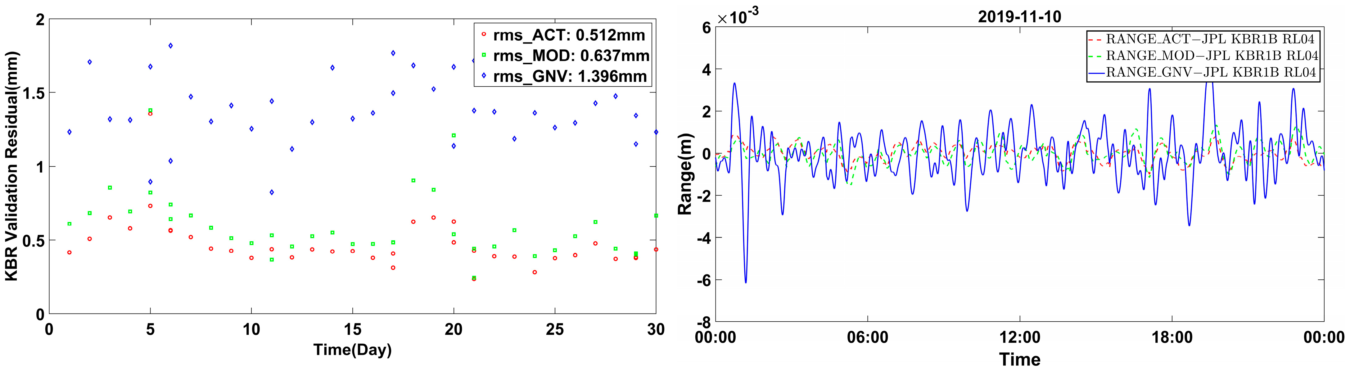
4.1.1. Comparison Analysis of Inter-Satellite Ranges Using Precise Orbit and Baseline Determination in the Time Domain

Figure 2 presents the KBR validation residuals using POD and PBD for November 2019. The left figure shows the daily RMS values, while the right figure details the KBR validation residuals from 10 November 2019. Throughout the month, the ACT method consistently yields the smallest KBR validation residuals, closely followed by the MOD method, with the GNV method performing the worst. The daily RMS of the KBR validation residuals for GNV is twice as large as those for ACT and MOD. The right figure highlights the distinct orbital periodicity in the KBR validation residuals of ACT and MOD, which is absent in the GNV method. Additionally, the KBR validation residuals on November 5th are notably higher compared to those from other days, as shown in the left figure.

4.1.2. Comparison Analysis of Inter-Satellite Ranges Using Precise Orbit and Baseline Determination in the Frequency Domain

Figure 3 illustrates spectral plots of the differences in the inter-satellite distances generated by three different orbit determination strategies compared to those measured by the KBR/LRI on 10 November 2019. RANGE_GNV represents the inter-satellite distance determined by the POD method, while RANGE_ACT and RANGE_MOD correspond to the inter-satellite distances obtained using the PBD method. From the figures, we observe that the energy distribution of the GNV method is more scattered. In contrast, the spectra of the ACT and MOD solutions exhibit distinct orbital periodicity characteristics. They outperform the GNV solution mainly between the orbital frequency and 2 mHz. Additionally, the right figure shows that the spectra of the three orbital products and the KBR, after subtracting the unscaled LRI distance data, all exhibit a significant peak of a nearly equal magnitude at 1 CPR. The Nuttall4 window is used for the LRI NO SCALE curve to adhere to the high dynamic range of LRI data products.

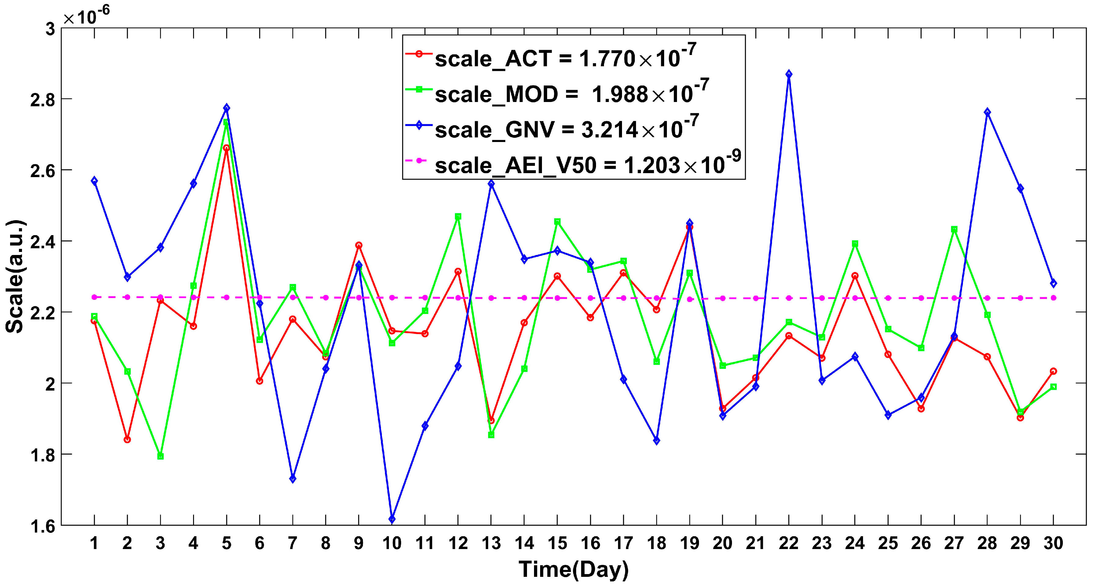
4.2. Analysis of the Energy-Based Scale Factor Estimation Method

4.2.1. Comparison Analysis of the Scale Factor

The scale factor estimations for November 2019 are illustrated in Figure 4, comprising estimates from SYSU, AEI, and JPL. SYSU employs energy-based methods for scale factor estimation, while AEI V50 and JPL rely on the cross-calibration approach and AEI V54 uses an exponent model. In the figure, the red curve denotes the scale factor estimated by SYSU, and the green, blue, and magenta curves, respectively, represent the scale factor values from JPL, AEI V50, and AEI V54. All three institutions use their own LRI1B data along with the KBR1B data generated by JPL for estimation. It can be observed from the graph that the overall consistency of the scale factor estimates from the three institutions is good, with the magnitude of the scale factor being roughly similar, except for on 24 November 2019. This is attributed to the occurrence of mega phase jumps in the LRI data on 24 November 2019, which JPL failed to adequately handle. In contrast, SYSU and AEI both eliminated these outliers, resulting in a more stable scale factor value. There is also a noticeable fluctuation in the scale factor on 19 November 2019, particularly pronounced in AEI’s V50 data. AEI refers that some noise from timing couples into the scale factor estimation [15]. In contrast, SYSU uses the spectral method, which decouples the scale and time delay, ensuring that the scale estimation remains unaffected. In summary, the energy-based scale factor estimation method has been proven effective. The scale factors estimated by the energy-based method are generally stable.

We randomly select three additional months of data to validate the energy method.

Table 1. Comparisons of scale factors from SYSU and AEI V50.

Month	Mean_SYSU_FREQ	Mean_AEI_V50	STD_SYSU	STD_AEI_V50
2020-10	2.235 × 10−6	2.235 × 10−6	4.983 × 10−9	3.153 × 10−9
2021-09	2.226 × 10−6	2.226 × 10−6	3.922 × 10−9	3.551 × 10−9
2022-06	2.588 × 10−6	2.590 × 10−6	9.759 × 10−9	8.747 × 10−9

shows that the scale factor values estimated using the energy method are highly consistent with the AEI V50 product, confirming the method’s effectiveness.

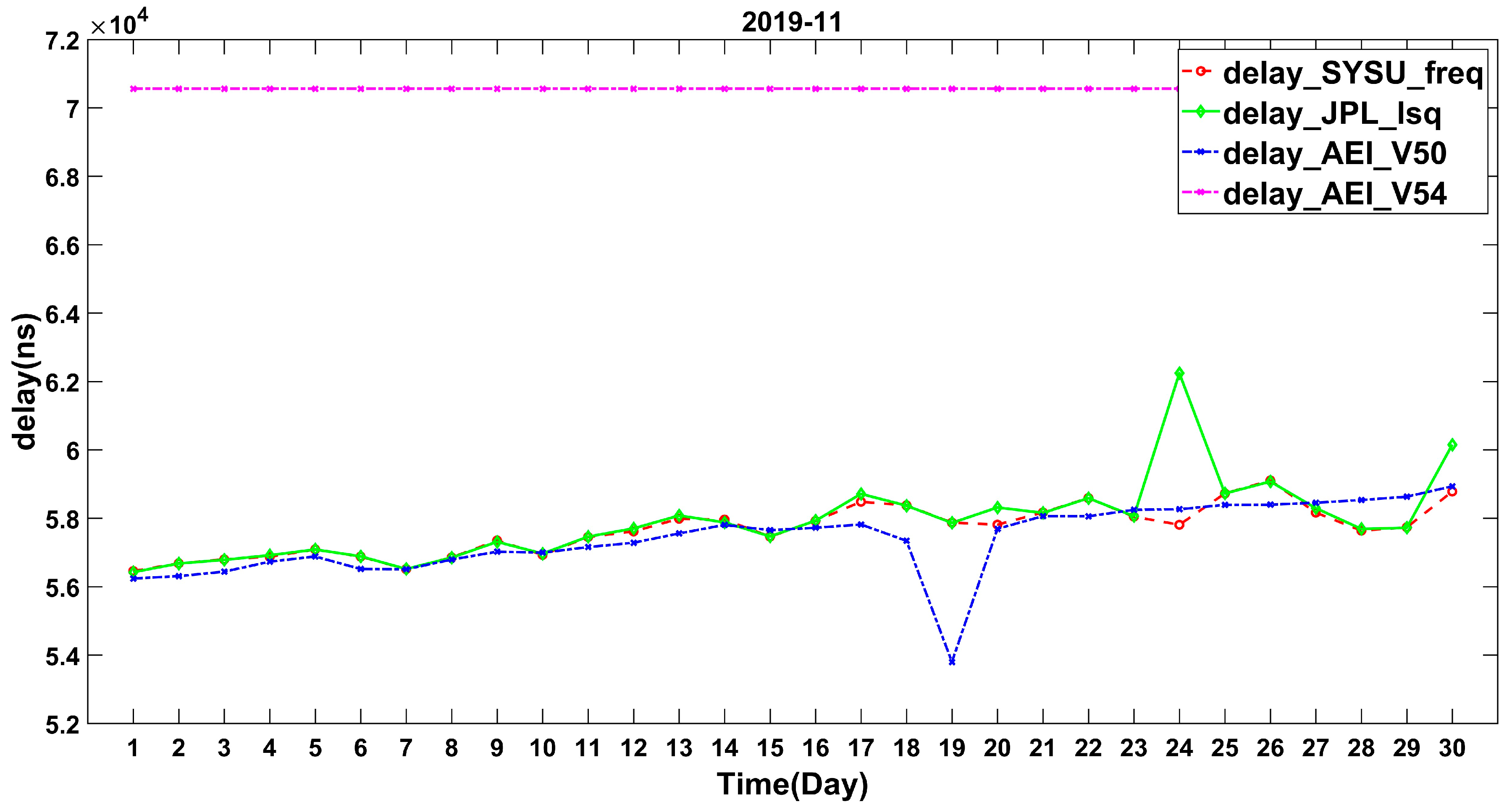
4.2.2. Comparison Analysis of the Time Shift

The time shift estimation for the entire month of November 2019 is illustrated in Figure 5, comprising estimates from SYSU, AEI, and JPL. In the figure, the red, green, blue, and magenta curves, respectively, represent the time shift values from SYSU, JPL, AEI V50, and AEI V54. The first three products use their own LRI1B data along with the KBR1B data generated by JPL to estimate the time shift. In contrast, AEI V54 uses a constant time shift of 70.54 µs because there is no physical or technical reason for the LRI time tags to vary with the KBR, as both are driven by the same USO clock [15]. It can be observed from the graph that overall consistency in the delay estimation is observed except for on 19 November 2019 and 24 November 2019. The time smooth algorithm used by AEI results in slight discrepancies compared to the estimates of JPL and SYSU. On the 24th, a mega jump occurs, driven by the sensitivity of the least squares method to outliers, thereby impacting the accuracy of the time shift estimation. The estimated time delay for AEI on 19 November 2019 also exhibits abrupt variations akin to those observed in the scale factor. The specific reasons for this were analyzed in the previous section.

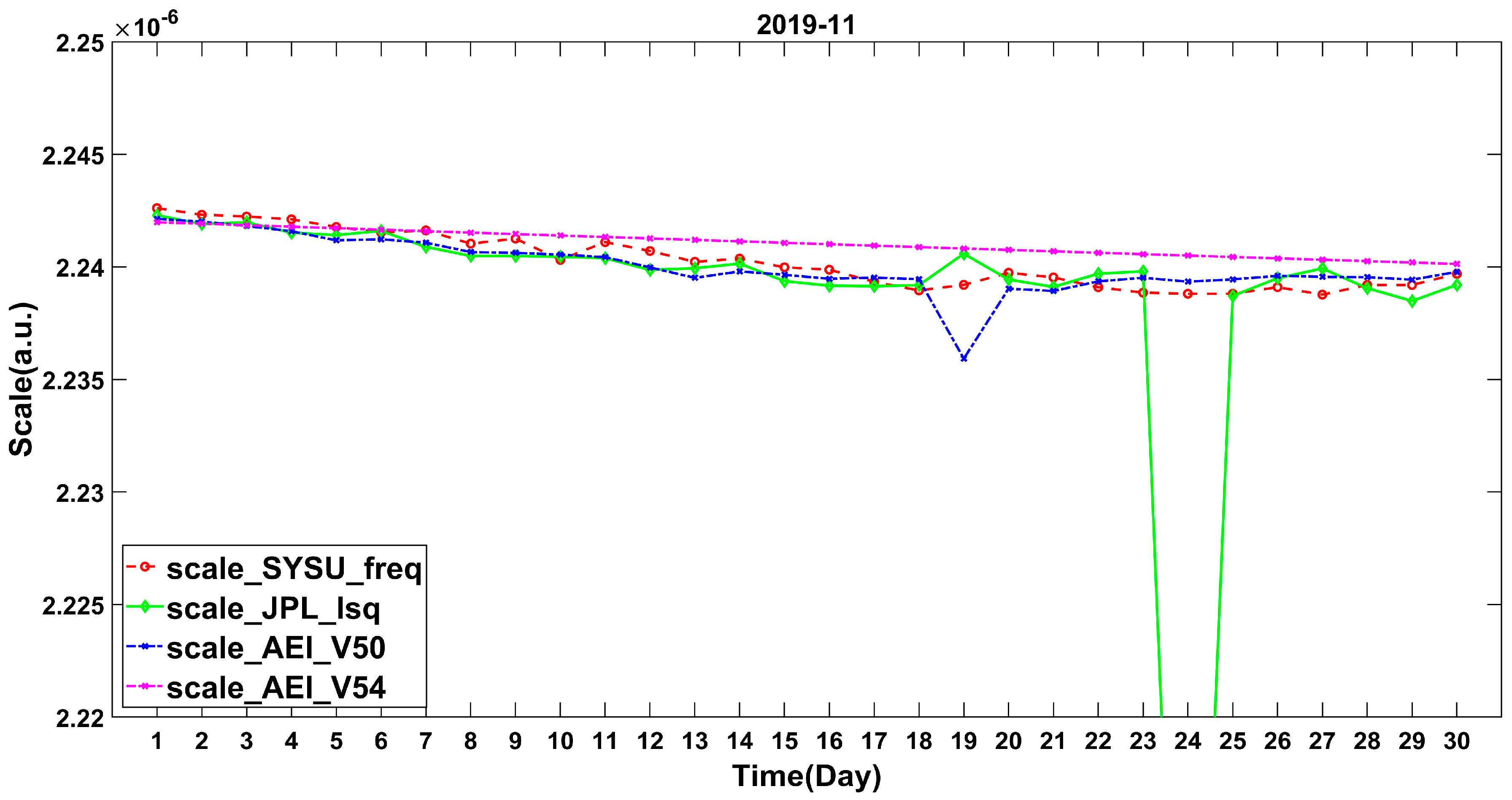
4.3. Comparison Analysis of the Proposed Method

Based on the proposed method, the SYSU LRI1B V01 datasets are produced. To validate the effectiveness of the proposed data preprocessing method, three comparative analyses are conducted on the estimation results of the scale factor and the instantaneous range.

4.3.1. Comparison Analysis of the Scale Factor

Figure 6 illustrates the results of the scale factor estimation using POD and PBD solutions for orbit determination in November 2019 based on the proposed method. The magenta curve represents the scale factor estimated by AEI LRI1B V50. The red curve, labeled as scale_ACT, represents the scale factor estimated by the energy method using instantaneous ranges obtained from relative orbit determination with accelerometer data. The green curve, labeled as scale_MOD, represents the scale factor estimated by the energy method using instantaneous ranges obtained from relative orbit determination with prior model data. The blue curve, labeled as scale_GNV, represents the scale factor estimated by the energy method using instantaneous ranges obtained from the JPL GNV1B RL04 data.

From the graph, it can be observed that the STD of scale factors from the POD and PBD products are two orders of magnitude higher than that of scale_AEI. The scale factors estimated using the GNV1B method exhibit apparently larger outlier values compared to the scale factors estimated from the two baseline products on days 7, 10, 22, and 28. Additionally, the STD of the scale factors obtained from the GNV1B method is approximately 1.5 times higher than those from the baseline products. Among these two baseline methods, the scale factors estimated using the ACT approach show slightly higher precision compared to those estimated by the MOD method.

Furthermore, there is good overall consistency in scale factor estimation using orbit baseline solutions, generally within an order of magnitude of (2.2 ± 0.2) × 10⁻⁶. In theory, smaller KBR residuals signify a higher orbit quality, leading to scale factor estimates closer to those published by AEI. Conversely, larger KBR residuals typically indicate poorer scale factors. While this holds true in most cases, there are examples such as that on 5 November 2019, where the baseline product KBR residuals exceeded 0.8 mm (as depicted in Figure 2), resulting in the poorest scale factor estimates. The accuracy of scale factor estimation is not strictly proportional to the baseline product KBR residuals. For instance, on 13 November 2019, the KBR residuals for the ACT method were 0.4 mm, and for the MOD method, they were 0.5 mm, yet the scale factor estimation only reached 1.89 × 10⁻⁶. This discrepancy stems from lower orbit precision, introducing some uncertainty when jointly estimating with high-precision LRIs. Consequently, data fluctuations near theoretical values may occur.

Currently, the scale factor uncertainty obtained from our baseline products can only reach 10⁻⁷, which does not yet meet the requirement for the laser frequency stability to be better than 10⁻⁸ for the next generation of gravity satellites. However, with further advancements in orbit determination technology and the stability of the GPS receiver improving, there is potential for this precision to be improved in the future.

4.3.2. Comparison Analysis of Instantaneous Ranges with AEI LRI1B

This study compares the LRI instantaneous ranges obtained from the proposed method by SYSU, JPL, and AEI in both the time and frequency domains. Figure 7 illustrates this comparison for three specific days: 1 November, 5 November, and 7 November. The selection of 5 November was due to the poor quality of orbit data on that day, while 1 November and 7 November were chosen because all the products (JPL, AEI, and SYSU) actually do agree on that day. Such an analysis has been performed to set the baseline of the comparison of the three.

The comparative results in both the time and frequency domains between the LRI1B products derived from two different orbits and those provided by the AEI/JPL are presented above, with frequency domain comparisons on the right and time domain comparisons on the left. The black curve represents the design noise level of the GRACE-FO LRI. Due to the poor quality of the scale factor obtained from JPL GNV1B, we excluded it from further comparisons. To differentiate between SYSU’s original data preprocessing quality and those of JPL and AEI, we use the SYSU_FREQ curve, which employs a scale factor derived from the energy method applied to the LRI1B and KBR1B. For the frequency domain, we utilize an amplitude spectrum, which is in units of [m].

We plot the corresponding noise curves according to the relationship between the ASD and AS [21]. The FFT points are equal to the total length of the input data. For LRI1B data at a 0.5 Hz data rate, the ENBW is approximately = 1.5 (for Hamming window) × 0.5/43,200 = 17.36 µHz.

From the time domain plots, it is evident that the instantaneous range differences caused by the scale factors are minimal. On 5 November, the day with the highest KBR validation residuals, the instantaneous range differences are an order of magnitude worse than the differences between the JPL and AEI instantaneous ranges. However, on the other two days, the differences are relatively small. Although the scale factor estimation error affects all the spectral frequencies equally, the differences are more pronounced in the low-frequency range. The high-frequency spectra of the SYSU products exhibit more spikes compared to the AEI products, likely due to the less refined phase jump handling by SYSU. However, this paper does not focus on phase jump processing.

Table 2. Comparison of scale factors and KBR residuals from baseline methods. On 5 November, there are two values recorded due to breaks in the KBR phase on that day.

Date	Scale_ACT	Scale_MOD	RMS_ACT (mm)	RMS_MOD (mm)
1 November 2019	2.175 × 10−6	2.185 × 10−6	0.4	0.6
5 November 2019	2.661 × 10−6	2.734 × 10−6	0.8/1.3	1.6/0.8
7 November 2019	2.180 × 10−6	2.270 × 10−6	0.5	0.6

lists some example dates of the estimated scale factors and the corresponding RMS values of the KBR validation residuals. Referencing Table 2 and Figure 7, we find that when the KBR validation residuals are lower than 0.8 mm, the accuracy of the baseline product generally consistently meets the LRI’s design noise requirements in the frequency band of 2 mHz to 0.1 Hz. However, on occasions when the KBR validation residuals are larger than 0.8 mm, such as on 5 November 2019, the estimated scale factor deviation fails to meet the design noise curve standards at the lowest frequency in the designed noise band.

4.3.3. Comparison Analysis of Instantaneous Ranges with JPL KBR1B

From the previous section, it is evident that the scale factors estimated using orbit data have little impact on the high-frequency range. Given that the scale factor is necessary at low frequencies, we examined its impact on the low-frequency range by subtracting the LRI product from the KBR1B RL04 product. The reason for subtracting the KBR is that the KBR ranging signal is more accurate at low frequencies compared to the LRI ranging signal because the KBR frequency is generated by multiplying the USO frequency, and the USO frequency variations can be obtained from the CLK1B product, derived from precise orbit determination. Similarly, we selected data from November 2019 and plotted their time domain and frequency domain representations below.

Figure 8 shows that SYSU_FREQ and JPL LRI1B exhibit a consistent time domain performance. Compared to the KBR residuals of the AEI LRI, the KBR residuals of SYSU_FREQ/the JPL LRI show a crossing characteristic centered at noon, suggesting that AEI V50 uses a smoothing interpolation of the scale factor and the time shift at noon each day. Additionally, the residuals show pronounced 1 CPR and 2 CPR oscillations in JPL LRI1B/SYSU_FREQ and LRI1B V50 with an amplitude of a few microns [22], while the baseline product exhibits only 1 CPR oscillations with a large amplitude of residuals in the time domain.

In the frequency domain, the difference between the baseline products and the other products at 1 CPR is significant, diminishes markedly at 2 CPR, and is noticeable only on the day when the baseline quality is at its worst after 2 CPR. Under normal baseline quality conditions, the spectral amplitudes of the baseline products are less than two orders of magnitude higher at 1 CPR and less than one order of magnitude higher at 2 CPR compared to the other LRI products. However, on days when the baseline LRI product quality is at its worst, the spectral amplitudes of the baseline products exceed those of the other LRI products by more than two orders of magnitude at 1 CPR, while at 2 CPR, the difference is one order of magnitude.

The scale factors of SYSU_ACT and SYSU_MOD are estimated from the baseline products. Due to the baseline’s insufficient accuracy, these estimated scale factors are not precise. Consequently, after subtracting KBR1B from SYSU_ACT and SYSU_MOD, a residual 1 CPR signal remains, resulting in a visible 1 CPR oscillation in both the time and frequency domains. In contrast, SYSU_FREQ, JPL, and AEI V50 have more accurate scale factors, which effectively weaken the 1 CPR signal after subtracting KBR1B.

Before 2 CPR, both the JPL and AEI’s LRI1B products, compared to the baseline products, exhibit smaller noise but still fail to meet the noise design requirements. GRACE-like datasets are currently too noisy at such low frequencies due to tone errors, temperature, and other effects. Currently, the influence of 1 CPR variations can only be mitigated through kinematic empirical parameters during gravity field recovery [23].

5. Conclusions

This study explores data preprocessing methods from LRI1A to LRI1B based on the GRACE-FO LRI’s actual measurements. It addresses issues in scale factor estimation such as the nonlinearity of the objective function, as well as the model’s inability to be entirely independent of the KBR. Our proposed energy-based scale factor estimation method using inter-satellite baseline solutions aims to address these challenges, which is suited to roughly extracting the scale factor as a stochastic mean over several months. We conducted a comprehensive comparison of this method with JPL and AEI’s LRI1B products regarding the scale factor and instantaneous ranges of LRI1B, leading to the following conclusions:

The accuracy of scale factor estimation depends on the correctness of the data preprocessing procedure. Failure to remove mega jumps and outliers properly can result in significant deviations in the scale factor estimation. JPL’s scale factor contained outliers mainly due to inadequate handling of mega phase jumps.

The prevalent method currently used to cross-calibrate scale factors and time shifts relies on Taylor expansion of inter-satellite range differences. However, nonlinear terms in this approach may result in the absorption of some errors from the KBR/GPS system due to timing noise. Our proposed method tackles these challenges by estimating scale and time shifts step by step. Initially, we estimate the scale factor in the frequency domain, followed by an estimation of the time shift based on this factor. Notably, our method disentangles the scale and a potential time tag offset between the LRI and KBR data. Comparison with the AEI and JPL’s scale factors indicates that our method is both simple and effective.

With the next generation of gravity satellites no longer equipped with KBR microwave instruments, there is the need to resolve the issue of scale factor estimation methods relying on KBR data. We utilize both POD and PBD methods to calculate inter-satellite distances. Our findings indicate that PBD methods exhibit distinct orbital periodic variations in the frequency domain, and the scale factors estimated from inter-satellite distances obtained via the POD method have slightly higher uncertainty compared to those from the PBD method. We suggest using PBD solutions to estimate LRI scale factors. In most cases, when the KBR validation residuals are lower than 0.8 mm, the SYSU LRI1B baseline products exhibit residuals below the payload design accuracy thresholds in the frequency band of 2 mHz to 0.1 Hz, meeting the precision requirements for gravity field inversion. Nevertheless, the results from a month of data comparison demonstrate the scale factor uncertainty obtained from our baseline products can only reach 10⁻⁷, which does not yet meet the requirement for the laser frequency stability to be better than 10⁻⁸ for the next generation of gravity satellites. However, with further advancements in orbit determination technology and the stability of the GPS receiver improving, there is potential for this precision to be improved in the future. Currently, this method appears to be suitable for roughly extracting the scale factor as a stochastic mean over several months or serving as a backup validation strategy for future missions.

In summary, our research on LRI data preprocessing, particularly the treatment of scale factors, holds significant implications for the data processing, gravity field inversion, and scientific applications of GRACE-FO and future gravity satellite missions.

References

1. Kornfeld, R.P.; Arnold, B.W.; Gross, M.A.; Dahya, N.T.; Klipstein, W.M.; Gath, P.F.; Bettadpur, S. GRACE-FO: The Gravity Recovery and Climate Experiment Follow-On Mission. J. Spacecr. Rocket. 2019, 56, 931–951. [Google Scholar] [CrossRef]
2. Sheard, B.S.; Heinzel, G.; Danzmann, K.; Shaddock, D.A.; Klipstein, W.M.; Folkner, W.M. Intersatellite laser ranging instrument for the GRACE follow-on mission. J. Geod. 2012, 86, 1083–1095. [Google Scholar] [CrossRef]
3. Flechtner, F.; Neumayer, K.-H.; Dahle, C.; Dobslaw, H.; Fagiolini, E.; Raimondo, J.-C.; Güntner, A. What Can be Expected from the GRACE-FO Laser Ranging Interferometer for Earth Science Applications? Surv. Geophys. 2016, 37, 453–470. [Google Scholar] [CrossRef]
4. Massotti, L.; Di Cara, D.; del Amo, J.; Haagmans, R.; Jost, M.; Siemes, C.; Silvestrin, P. The ESA Earth Observation Programmes Activities for the Preparation of the Next Generation Gravity Mission. In Proceedings of the AIAA Guidance, Navigation, and Control (GNC) Conference, Guidance, Navigation, and Control and Co-located Conferences, Boston, MA, USA, 19–22 August 2013; American Institute of Aeronautics and Astronautics: Reston, VA, USA, 2013. [Google Scholar] [CrossRef]
5. Gong, Y.; Luo, J.; Wang, B. Concepts and status of Chinese space gravitational wave detection projects. Nat. Astron. 2021, 5, 881–889. [Google Scholar] [CrossRef]
6. Dionisio, S.; Anselmi, A.; Bonino, L.; Cesare, S.; Massotti, L.; Silvestrin, P. The “Next Generation Gravity Mission”: Challenges and consolidation of the system concepts and technological innovations. In Proceedings of the 2018 SpaceOps Conference, Marseille, France, 28 May–1 June 2018. [Google Scholar] [CrossRef]
7. Yan, Y.; Müller, V.; Heinzel, G.; Zhong, M. Revisiting the light time correction in gravimetric missions like GRACE and GRACE follow-on. J. Geod. 2021, 95, 48. [Google Scholar] [CrossRef]
8. Wen, H.Y.; Kruizinga, G.; Paik, M.; Landerer, F.; Bertiger, W.; Sakumura, C.; Bandikova, T.; Mccullough, C. Gravity Recovery and Climate Experiment (GRACE) Follow-On (GRACE-FO) Level-1 Data Product User Handbook; JPL: Pasadena, CA, USA, 2019; Volume D-56935. [Google Scholar]
9. Misfeldt, M.; Müller, V.; Heinzel, G.; Danzmann, K. Alternative Level 1A to 1B Processing of GRACE Follow-On LRI data. In Proceedings of the Copernicus Meetings, Online, 3–8 May 2020; p. 15569. [Google Scholar]
10. Misfeldt, M. Data Processing and Investigations for the GRACE Follow-On Laser Ranging Interferometer. Master’s Thesis, Leibniz University Hannover, Hanover, Germany, 2019. [Google Scholar]
11. Müller, L. Generation of Level 1 Data Products and Validating the Correctness of Currently Available Release 04 Data for the GRACE Follow-on Laser Ranging Interferometer. Master’s Thesis, Leibniz Universität Hannover, Hannover, Germany, 2021. [Google Scholar]
12. Misfeldt, M.; Müller, V.; Müller, L.; Wegener, H.; Heinzel, G. Scale Factor Determination for the GRACE Follow-On Laser Ranging Interferometer Including Thermal Coupling. Remote Sens. 2023, 15, 570. [Google Scholar] [CrossRef]
13. Rees, E.R.; Wade, A.R.; Sutton, A.J.; Spero, R.E.; Shaddock, D.A.; McKenzie, K. Absolute frequency readout derived from ULE cavity for next generation geodesy missions. Opt. Express 2021, 29, 26014–26027. [Google Scholar] [CrossRef] [PubMed]
14. Klinger, B.; Mayer-Gürr, T.A.A.A.B. The role of accelerometer data calibration within GRACE gravity field recovery: Results from ITSG-Grace2016. Adv. Space Res. 2016, 58, 1597–1609. [Google Scholar] [CrossRef]
15. Malte Misfeldt, L.M.; Müller, V. AEI LRI1B and RTC1B Release Notes; Max-Planck Institute for Gravitational Physics (Albert Einstein Institute): Hanover, Germany, 2022. [Google Scholar]
16. Wei, C.; Shao, K.; Gu, D.; Zhang, Z.; Zhu, J.; An, Z.; Wang, J. Enhanced orbit and baseline determination for formation-flying LEO satellites with spaceborne accelerometer measurements. J. Geod. 2023, 97, 64. [Google Scholar] [CrossRef]
17. Mayer-Guerr, T.; Behzadpour, S.; Eicker, A.; Ellmer, M.; Koch, B.; Krauss, S.; Pock, C.; Rieser, D.; Strasser, S.; Suesser-Rechberger, B.; et al. GROOPS: A software toolkit for gravity field recovery and GNSS processing. Comput. Geosci. 2021, 155, 104864. [Google Scholar] [CrossRef]
18. Proakis, J.G.; Manolakis, D.G. Digital Signal Processing Principles, Algorithms and Applications; Pearson Education: New Delhi, India, 2003. [Google Scholar]
19. Sun, Y.; Ditmar, P.; Riva, R. Observed changes in the Earth’s dynamic oblateness from GRACE data and geophysical models. J. Geod. 2016, 90, 81–89. [Google Scholar] [CrossRef] [PubMed]
20. Peidou, A.; Landerer, F.; Wiese, D.; Ellmer, M.; Fahnestock, E.; McCullough, C.; Spero, R.; Yuan, D.N. Spatiotemporal Characterization of Geophysical Signal Detection Capabilities of GRACE-FO. Geophys. Res. Lett. 2021, 49, e2021GL095157. [Google Scholar] [CrossRef]
21. Heinzel, G.; Rüdiger, A.; Schilling, R. Spectrum and Spectral Density Estimation by the Discrete Fourier Transform (DFT), Including a Comprehensive List of Window Functions and Some New Flat-Top Windows; Max Planck Institutes: Hannover, Germany, 2002; Volume 12. [Google Scholar]
22. Müller, V.; Hauk, M.; Misfeldt, M.; Müller, L.; Wegener, H.; Yan, Y.; Heinzel, G. Comparing GRACE-FO KBR and LRI Ranging Data with Focus on Carrier Frequency Variations. Remote Sens. 2022, 14, 4335. [Google Scholar] [CrossRef]
23. Zhou, H.; Luo, Z.; Zhou, Z.; Li, Q.; Zhong, B.; Lu, B.; Hsu, H. Impact of Different Kinematic Empirical Parameters Processing Strategies on Temporal Gravity Field Model Determination. J. Geophys. Res. Solid Earth 2018, 123, 10252–10276. [Google Scholar] [CrossRef]
Figure 1. Schematic diagram of POD and PBD solutions for scale factor estimation.
Remotesensing 16 02523 g001
Figure 2. Daily RMS of KBR validation residuals in November 2019 (left) and KBR validation residuals on November 10 (right). The blue dots and curve represent the daily RMS of KBR validation residuals per arc and KBR validation residuals generated by JPL’s GNV1B orbit product and KBR, respectively. The green dots and curve are generated by the empirical non-conservative force model. The red dots and curve are generated by accelerometer measurements. In the left figure, some dates have multiple points due to breaks in the KBR phase on those days, with each segment producing its own RMS value.
Remotesensing 16 02523 g002
Figure 3. Comparison of three types of inter-satellite instantaneous ranges obtained by POD and PBD with KBR instantaneous range (left) and unscaled LRI range (right) in the frequency domain.
Remotesensing 16 02523 g003
Figure 4. Comparison of scale factor estimation results from SYSU, AEI, and JPL. It is notable that AEI estimates time shifts and scale factors daily, which are then interpolated to a 10 Hz rate. During this comparison, we opted for the daily average values of scale factor and time shift provided by the AEI. We obtained the AEI scale factor using the formula 1 − (c/(mean (AEILRI1B.iono_corr) × 2)/fM). The mean values of the scale factors derived from SYSU, JPL, AEI V50, and AEI V54 are 2.240 × 10⁻⁶, 2.238 × 10⁻⁶, 2.240 × 10⁻⁶, and 2.241 × 10⁻⁶ in November 2019, respectively. The STD values of the scale factors derived from SYSU, JPL, AEI V50, and AEI V54 in November 2019 are 1.549 × 10⁻⁹, 8.873 × 10⁻⁹, 1.203 × 10⁻⁹, and 5.621 × 10⁻¹⁰.
Remotesensing 16 02523 g004
Figure 5. Comparison of time shift estimation results from SYSU, the AEI, and JPL. We obtained the JPL time shift by subtracting CLK1B.eps_time from LLK1B.eps_time and then taking the average.
Remotesensing 16 02523 g005
Figure 6. Scale factors obtained from POD and PBD solutions compared with the AEI’s scale factors. It is worth noting that POD and PBD can sometimes introduce anomalies in orbit due to carrier-phase ambiguity fixing errors. These errors can affect the accuracy of scale factor estimation, necessitating the exclusion of periods with carrier-phase ambiguity fixing errors before scale factor estimation. The mean values of the scale factors derived from SYSU_ACT, SYSU_MOD, JPL_GNV, and AEI V50 are 2.147 × 10⁻⁶, 2.186 × 10⁻⁶, 2.227 × 10⁻⁶, and 2.240 × 10⁻⁶, respectively. The STD values of the scale factors derived from SYSU_ACT, SYSU_MOD, JPL_GNV, and AEI V50 are 1.770 × 10⁻⁷, 1.988 × 10⁻⁷, 3.214 × 10⁻⁷, and 1.203 × 10⁻⁹.
Remotesensing 16 02523 g006
Figure 7. Time (left) and frequency (right) comparisons of LRI1B instantaneous range from SYSU, JPL, and AEI. The dots denote a 1 µm tone amplitude, being the tone error requirement for the LRI at specific frequencies.
Remotesensing 16 02523 g007aRemotesensing 16 02523 g007b
Figure 8. Time (left) and frequency (right) comparisons of LRI1B instantaneous range difference from JPL KBR1B.
Remotesensing 16 02523 g008