Article

An Efficient Sparse Recovery STAP Algorithm for Airborne Bistatic Radars Based on Atomic Selection under the Bayesian Framework

National Key Laboratory of Radar Signal Processing, Xidian University, Xi’an 710071, China
*
Author to whom correspondence should be addressed.
Remote Sens. 2024, 16(14), 2534; https://doi.org/10.3390/rs16142534
Submission received: 9 May 2024 / Revised: 27 June 2024 / Accepted: 8 July 2024 / Published: 10 July 2024

Abstract

:
The traditional sparse recovery (SR) space-time adaptive processing (STAP) algorithms are greatly affected by grid mismatch, leading to poor performance in airborne bistatic radar clutter suppression. In order to address this issue, this paper proposes an SR STAP algorithm for airborne bistatic radars based on atomic selection under the Bayesian framework. This method adopts the idea of atomic selection for the process of Bayesian inference, continuously evaluating the contribution of atoms to the likelihood function to add or remove atoms, and then using the selected atoms to estimate the clutter support subspace and perform sparse recovery in the clutter support subspace. Due to the inherent sparsity of clutter signals, performing sparse recovery in the clutter support subspace avoids using a massive number of atoms from an overcomplete space-time dictionary, thereby greatly improving computational efficiency. In airborne bistatic radar scenarios where significant grid mismatch exists, this method can mitigate the performance degradation caused by grid mismatch by encrypting grid points. Since the sparse recovery is performed in the clutter support subspace, encrypting grid points does not lead to excessive computational burden. Additionally, this method integrates out the noise term under a new hierarchical Bayesian model, preventing the adverse effects caused by inaccurate noise power estimation during iterations in the traditional SR STAP algorithms, further enhancing its performance. Our simulation results demonstrate the high efficiency and superior clutter suppression performance and target detection performance of this method.

1. Introduction

The airborne bistatic radar uses a transmit–receive separated system, which allows the transmitter to be placed at a location far from the battlefield and the receiver to be placed in the area of interest. Compared to ordinary airborne monostatic radars, airborne bistatic radars have outstanding advantages such as rich information acquisition, a long operational range, high security, strong anti-interference capabilities, and an anti-interception ability [1,2,3]. However, the clutter properties of airborne bistatic radars are very complex. Firstly, the spatial–temporal coupling properties of ground clutter in airborne bistatic radars depend on the spatial positions and orientations of the transmit and receive antennas and the velocity vectors of the transmit and receive platforms to form a highly complex nonlinear two-dimensional function. Secondly, in the airborne bistatic radar scenario, the clutter distribution in different range cells is different, and this variation is very drastic, exhibiting characteristics of non-stationarity over distance [4,5]. According to the Reed–Mallett–Brennan (RMB) rule [6], to ensure that the average signal-to-clutter-plus-noise ratio loss of a space-time adaptive processing [7,8,9,10,11,12,13,14,15,16,17] (STAP) filter is less than 3dB, the number of samples required to estimate the clutter covariance matrix (CCM) is at least twice the system’s degrees of freedom (DOFs). Due to the limited independent and identically distributed (IID) samples for STAP in bistatic airborne radars, it becomes very challenging to perform clutter suppression.
One commonly used method for suppressing non-stationary clutter signals in airborne bistatic radars is range domain localization, where the basic idea is to allow training samples and weight vectors to vary with distance, such as the sliding window method [18,19] and segmented processing method [20]. These methods all assume that clutter data are locally stationary within a certain range. However, due to the severe non-stationary characteristics of airborne bistatic radar clutter over distance, these methods have limited abilities in terms of clutter suppression. Another method is to preprocess the non-stationary clutter signal into a stationary clutter signal or a locally stationary clutter signal, and then use conventional STAP methods for further processing. The Doppler compensation (DC) method [21] and the high-order Doppler compensation (HODC) method [22] both involve the spectral shifting of clutter signals into the Doppler domain. The angle Doppler compensation (ADC) method [23] and the adaptive angle Doppler compensation (A2DC) method [24,25] involve signal spectral shifting into the two-dimensional domain formed by the spatial frequency and Doppler frequency, but these methods only compensate for clutter in the main lobe and do not compensate for clutter in the sidelobes. The scale transformation (SC) method [26] and the joint spatial–temporal interpolation (JSTI) method [27,28] change the original spatial–temporal vector form, enabling movement and scaling within a two-dimensional angle-Doppler plane while simultaneously compensating for the main lobe and sidelobes’ clutter spectra. The downside is that these methods require a large amount of computation and are not sufficiently robust. The derivative-based updating (DBU) method [29] uses different adaptive weights for clutter suppression at different distances, expressing the adaptive weight vector as a linear function of distance. However, due to its assumption being not very reasonable, its clutter suppression performance in practical applications is not very ideal. Furthermore, unfortunately, in the case of limited training samples, all these preprocessing methods will become ineffective.
In recent years, the development of sparse recovery (SR) technology [30,31,32,33,34,35,36] has provided new ideas for suppressing non-stationary clutter in airborne radars. Many SR STAP methods [37,38,39,40,41,42,43] have been proposed. The SR STAP technology leverages the inherent sparsity of clutter and can reconstruct the CCM using only a small number of training samples. Then, clutter suppression and target detection processing can be performed using the reconstructed CCM. Ślesicka and Kawalec [40] propose an SR STAP algorithm based on orthogonal matching pursuit (OMP). Yang et al. [41] introduce an SR STAP algorithm based on the focal underdetermined system solver (FOCUSS). An SR STAP algorithm based on iterative adaptive approach (IAA) technology is introduced in reference [42]. However, none of these algorithms consider the grid mismatch problem that may exist when constructing the dictionary. When there is a deviation between clutter scattering points and pre-divided grid points, i.e., in the case of grid mismatch, the performance of these algorithms will deteriorate sharply. When applying these SR STAP algorithms to clutter suppression in airborne bistatic radars, there is a serious grid mismatch issue that prevents these algorithms from achieving good performance. The SR STAP algorithm proposed in reference [43] is based on the atomic norm, which does not involve a dictionary matrix. It can directly perform sparse recovery in the continuous domain based on the Vandermonde decomposition, avoiding the issue of grid mismatch. However, a drawback is that the algorithm requires a CVX solver [44] for solving, resulting in high computational complexity.
In traditional sparse recovery algorithms, the SBL algorithm, in multiple measurement vector (MMV) cases (MSBL), has been proven to be a performance-robust SR technique that does not require setting regularization parameters and still performs well when there is strong correlation among atoms in the dictionary [45,46,47,48]. In recent years, a large number of SR STAP algorithms based on the MSBL technique have been proposed [49,50,51,52,53,54,55,56]. Duan et al. [49] were the first to present an SR STAP algorithm based on the MSBL technique (MSBL-STAP). However, the MSBL-STAP algorithm faces the issues of a slow convergence speed and high computational complexity. In order to improve the efficiency of the MSBL-STAP algorithm, Liu et al. [50] derived an iterative reweighted SR STAP algorithm under the Bayesian framework. This method significantly improves the convergence speed, but it does not reduce the computational complexity of a single iteration. Cui et al. [51] use tensor computations to replace vector computations, breaking down the solving of large-scale matrices into a series of smaller ones, thus reducing computational complexity. However, this method has a limited ability to decrease the computational complexity of a single iteration. Utilizing the Toeplitz-block-Toeplitz structure of the covariance matrix in the iterative process of the MSBL-STAP algorithm, Liu et al. [52] propose a fast MSBL-STAP algorithm based on G-S decomposition. This method significantly reduces computational complexity but is only applicable to the side-looking array, which greatly limits its applicability. Wang et al. [53] propose a new MSBL-STAP method based on statistical thresholds, which adaptively differentiates between useful and useless atoms in the space-time dictionary, thereby improving the efficiency of the MSBL-STAP algorithm. Cao et al. [54] derive the MSBL-STAP algorithm in the beam domain. Although these two algorithms can reduce computational complexity, they also bring a certain level of performance loss. These fast algorithms are beneficial for the real-time operation of the MSBL-STAP algorithm. However, when grid mismatch problems exist, all these algorithms fail. Cui et al. [55] propose a gridless MSBL-STAP method that parameterizes the marginal likelihood function of the MSBL-STAP algorithm. This method can directly estimate the CCM with the Toeplitz-block-Toeplitz structure under the continuous domain. However, this method is essentially equivalent to the weighted atomic norm STAP algorithm. It requires the use of the CVX solver multiple times, resulting in high computational complexity. Zhang et al. [56] propose a gridless MSBL-STAP method where the Toeplitz-block-Toeplitz-structured CCM can be estimated by solving an optimization problem which is based on the stochastic maximum likelihood criterion. However, this method needs an SDP solver [44] to solve the semidefinite programming problem, which also brings a huge computational burden. In scenarios with grid mismatch issues, the clutter suppression performance of these two algorithms is slightly better than the MMV SR STAP algorithm based on the atomic norm (MANM-STAP). However, they have a much higher computational complexity than MANM-STAP, which limits their practical applications. In order to apply the MSBL technique to clutter suppression in airborne bistatic radars, this paper proposes an SR STAP algorithm for airborne bistatic radars based on atomic selection under the Bayesian framework. This algorithm adopts the idea of atomic selection in the process of Bayesian inference, continuously evaluating the contribution of each atom to the likelihood function to add or remove atoms. It uses the selected atoms to estimate the clutter support subspace and performs sparse recovery in the clutter support subspace, avoiding high-dimensional matrix inversion operations during the learning process and significantly improving the algorithm’s computational efficiency. The algorithm reduces the performance loss caused by grid mismatch by encrypting grid points. Since this method performs sparse recovery in the clutter support subspace, encrypting grid points does not impose a high computational burden. However, when encrypting grid points to reduce grid mismatch, the number of atoms in the dictionary is much larger than the DOFs. According to reference [48], at this point, noise updates may be inaccurate, which can affect algorithm’s performance. To address this issue, this method integrates out the noise term under a new hierarchical Bayesian model to avoid the adverse effects caused by inaccurate noise power estimations during the iterative process of the traditional MSBL-STAP algorithm.
The primary contributions of this work are outlined as follows:
(a)
An efficient SR STAP algorithm for airborne bistatic radars based on atomic selection under the Bayesian framework is proposed; it has low computational complexity and addresses the issue of grid mismatch when applying the MSBL-STAP algorithm to an airborne bistatic radar.
(b)
Under the new hierarchical Bayesian model, the noise term is integrated out to avoid the adverse effects caused by inaccurate noise power estimations in the iterative process of the traditional MSBL-STAP algorithm when the number of atoms in the dictionary is much larger than the system’s degrees of freedom under encrypted grid conditions, further improving the algorithm’s performance.
(c)
We conducted a large number of simulation experiments to validate the efficiency, clutter suppression performance and target detection performance of our algorithm. The simulation results show that, compared to other traditional STAP and SR STAP algorithms, our algorithm demonstrates high efficiency and good clutter suppression performance and target detection performance.
The remaining sections of the article are organized as follows: In Section 2, we first introduce the SR STAP signal model for airborne bistatic radars, and then we theoretically analyze the grid mismatch problem existing when applying the SR STAP algorithm to the airborne bistatic radar. In Section 3, we present the proposed algorithm. Section 4 analyzes the convergence and the computational complexity of the proposed algorithm. Simulation results are provided in Section 5 to demonstrate the superior performance of the proposed algorithm. The conclusion is given in Section 6.
Notation: Matrices are represented by bold uppercase letters, vectors are denoted by bold lowercase letters and scalars are indicated by italic letters. The sets and , respectively, represent real and complex numbers. The superscripts H and T denote the conjugate transpose and transpose operations, respectively. A unit matrix of size N K × N K is represented by I N K . The symbol represents the Kronecker product operation. The symbol represents a definition operation. diag a denotes a diagonal matrix where the elements of the vector a are placed along the diagonal. The operations Re x and Im x represent extracting the real part and the imaginary part of the vector x . C N and N represent the complex and real normal distribution. Gamma represents the real Gamma distribution. · 2 and · F are used to denote the l 2 norm and the Frobenius norm, respectively. 2 , 1 represents a l 2 , 1 mixed norm that can be defined as the summation of a column vector comprising the l 2 norm of individual row vectors.

2. Signal Model

2.1. Signal Model of SR STAP for Airborne Bistatic Radars

Figure 1 shows the geometry of an airborne bistatic radar system. We consider that both the transmitter and the receiver carry a pulse Doppler radar array, where the array is a uniform linear array (ULA) which is made up of N elements. The spacing between the elements is d = λ / 2 , where λ represents the wavelength. The angles between the array axis and the positive x-axis are α T and α R , respectively. The heights of the transmitting and receiving platforms are H T and H R , respectively. The angles between the platform velocity direction and the positive x-axis are β T and β R , respectively. In this airborne bistatic radar system, the pulse repetition frequency (PRF) is f r and K pulses are emitted in a coherent processing interval (CPI).
In airborne bistatic radar signal processing, ground clutter can be segmented into distinct iso-range ellipse rings. Each iso-range ring can be interpreted as the composite of N c independent and discrete clutter patches. Without considering the distance ambiguity, the radar clutter return of the entire L range bin can be modeled as
Y = y 1 , y 2 , , y L N K × L
where the clutter return of the l - th range bin y l can be represented as
y l = i = 1 N c σ i s i + n l = i = 1 N c σ i b f d i a f s i + n l
where σ i is the complex amplitude of the clutter echo of the i - th clutter patch and n l C N 0 , σ 2 I N K is the complex Gaussian noise vector. a f s i and b f d i are the spatial steering vector and the temporal steering vector of the i - th clutter patch, represented by
a f s i = 1 , exp j 2 π f s i , , exp j 2 π N 1 f s i T
b f d i = 1 , exp j 2 π f d i , , exp j 2 π K 1 f d i T
where f s i and f d i are the normalized spatial frequency and the normalized Doppler frequency of the i - th clutter patch, represented by
f s i = d cos φ R i λ
f d i = v T cos ψ T i λ f r + v R cos ψ R i λ f r
where v T and v R are the speeds of the transmitter and receiver; cos φ R i , cos ψ T i and cos ψ R i are the receiver array cone angle cosine, the transmitter speed cone angle cosine and the receiver speed cone angle cosine of the i - th clutter patch, represented by
cos φ R i = cos ϕ R i cos θ R i cos α R + cos ϕ R i sin θ R i sin α R
cos ψ T i = cos ϕ T i cos θ T i cos β T + cos ϕ T i sin θ T i sin β T
cos ψ R i = cos ϕ R i cos θ R i cos β R + cos ϕ R i sin θ R i sin β R
where θ T i and ϕ T i are the azimuth angle and elevation angle of the i - th clutter patch relative to the transmitter and θ R i and ϕ R i are the azimuth angle and elevation angle of the i - th clutter patch relative to the receiver.
Due to the low-rank nature of ground clutter [20], in the SR STAP framework, we can represent the clutter signal by using an overcomplete space-time dictionary and a sparse coefficient vector. Firstly, we uniformly discretize the continuous space-time plane into N s K d grids, where N s = ρ s N represents the number of grids in the spatial domain and K d = ρ d K represents the number of grids in the temporal domain, with ρ s > 1 and ρ d > 1 denoting the resolution scales. Then, the signal model (2) can be easily rewritten as
y l = A x l + n l
where A = s ( f d , 1 , f s , 1 ) , , s ( f d , K d , f s , N s ) = s 1 , s 2 , , s N s K d N K × N s K d is the constructed overcomplete space-time dictionary and x l N s K d × 1 is the sparse coefficient vector. And the clutter and noise echoes received from L range cells Y can be reformulated as the following SR STAP model:
Y = A X + N
where N = [ n 1 , n 2 , , n L ] N K × L is the noise matrix and X = [ x 1 , x 2 , , x L ] N s K d × L is the sparse coefficient matrix to be solved. We find that (11) is a typical sparse recovery signal model in the MMV case. Then, utilizing the l 2 , 1 mixed norm, the sparse solution matrix X can be derived by resolving the following optimization issue [49]:
min Y A X F 2 + ε X 2 , 1
where ε is a parameter used to balance the sparsity of the solution matrix X and the model error. Once we obtain the sparse coefficient matrix X , we can reconstruct the clutter plus noise covariance matrix (CNCM), represented by
R ^ = 1 L l = 1 L m = 1 N s K d x l , m 2 s m s m H + σ 2 I N K
where x l , m is the m - th component of x l . Then, based on the principle of a linearly constrained minimum variance (LCMV), we can obtain the optimal weight vector for STAP, represented by
w opt = R ^ 1 s t s t H R ^ 1 s t
where s t = b f d t a f s t denotes the space-time steering vector of the target.

2.2. Grid Mismatch Analysis

As shown in Figure 1, the coordinates of the transmitter are C T x T , y T , H T and the coordinates of the receiver are C R x R , y R , H R , thus the velocity direction vector of the transmitter is
v T = cos β T , sin β T , 0
and the velocity direction vector of the receiver is
v R = cos β R , sin β R , 0
and the axial vector of the receiver antenna array is
r = cos α R , sin α R , 0
The position coordinate of the i - th clutter patch on the l - th range ring is P x i , y i , 0 ; assuming the length of the line connecting the clutter patch P to the origin is r , then we can obtain
x i = r cos θ i y i = r sin θ i
The vector pointing from the transmitter to the clutter point P is
l T P = x i x T , y i y T , H T
The vector pointing from the receiver to the clutter point P is
l R P = x i x R , y i y R , H R
Then, the transmitter speed cone angle cosine and the receiver speed cone angle cosine of the i - th clutter patch can be written as
cos ψ T i = v T l T P v T l T P = r cos θ i x T cos β T + r sin θ i y T sin β T r cos θ i x T 2 + r sin θ i y T 2 + H T 2
cos ψ R i = v R l R P v R l R P = r cos θ i x R cos β R + r sin θ i y R sin β R r cos θ i x R 2 + r sin θ i y R 2 + H R 2
and the receiver array cone angle cosine of the i - th clutter patch can be written as
cos φ R i = r l R P r l R P = r cos θ i x R cos α R + r sin θ i y R sin α R r cos θ i x R 2 + r sin θ i y R 2 + H R 2
By substituting Equations (21) and (22) into Equation (6), we can obtain the normalized Doppler frequency of the i - th clutter patch, i.e.,
f d i = v T λ r cos θ i x T cos β T + r sin θ i y T sin β T r cos θ i x T 2 + r sin θ i y T 2 + H T 2 + v R λ r cos θ i x R cos β R + r sin θ i y R sin β R r cos θ i x R 2 + r sin θ i y R 2 + H R 2
By substituting Equation (23) into Equation (5), we can obtain the normalized spatial frequency of the i - th clutter patch, i.e.,
f s i = 2 v R λ r cos θ i x R cos α R + r sin θ i y R sin α R r cos θ i x R 2 + r sin θ i y R 2 + H R 2
From Equations (24) and (25), it can be seen that the distribution of clutter on the space-time two-dimensional plane is continuous and there exists a functional relationship between f d i and f s i . However, due to the complexity of the relationship between f d i and f s i , it is difficult for us to obtain their explicit function expression. But we can substitute the distance r and θ i into Equations (24) and (25). In this way, we can obtain all f d i and f s i and then we can plot the theoretical space-time two-dimensional distribution curve for a certain range bin.
In Figure 2, we plot the schematic diagram of the grid mismatch phenomenon under two different airborne bistatic radar configurations. These two airborne bistatic radar configurations are a transmitter and receiver on a collinear flight path and a transmitter and receiver on a parallel flight path, respectively. The red lines represent the theoretical space-time two-dimensional distribution curves of the clutter, and the intersection points of each vertical line and straight line are our preset grid points. From Figure 2, it can be seen that the distribution of the clutter of the airborne bistatic radars is continuous in the two-dimensional space-time plane, but the grid points we pre-divided on the space-time two-dimensional plane are discrete. Moreover, the majority of the two-dimensional distribution curves of the clutter fall outside the preset discrete grid points. This phenomenon is called grid mismatch. The fundamental reason for the existence of grid mismatch is that we have discretely divided the space-time two-dimensional plane in the SR STAP algorithm. When the grid mismatch phenomenon occurs, the SR STAP method, in order to reduce the fitting error brought about by the first term in Equation (12), will cause the algorithm to choose the atoms closest to the real clutter frequencies in the space-time dictionary to reconstruct the CNCM. This will lead to an inaccurate estimation of CNCM in the SR STAP algorithms, thereby affecting the clutter suppression ability of the SR STAP filter and the detection performance of slow-moving targets. Thus, in order to apply the SR STAP algorithm to bistatic airborne radars, the grid mismatch problem is a problem that must be resolved.

3. Proposed Algorithm

Due to the robust and excellent performance of MSBL, the MSBL-STAP algorithms have been widely studied in the scenario of airborne monostatic radars and proven to achieve superior clutter suppression performance [49,50,51,52,53,54,55,56]. However, in the scenario of airborne bistatic radars, traditional MSBL-STAP algorithms face the problem of grid mismatch; thus, they cannot suppress clutter well. To overcome this drawback, in this section, based on the Bayesian framework, we introduce an efficient MSBL-STAP algorithm based on atomic selection (ASMSBL-STAP) that can address the grid mismatch problem.

3.1. Hierarchical Bayesian Framework

In the traditional sparse Bayesian framework, a hierarchical prior model is assigned to the sparse coefficient matrix X to encourage sparsity [45]. Firstly, a Gaussian prior with a zero mean is assigned to the sparse coefficient matrix X ; thus, the probability density function (PDF) of X can be written as
p ( X ; γ ) = l = 1 L m = 1 N s K d C N x l , m | 0 , γ m
where γ = γ 1 , γ 2 , , γ N s K d T N s K d × 1 is the unknown hyperparameter vector. All elements in each row of X are controlled by the same hyperparameter, i.e., all columns in X have the same sparse structure. Then, to promote the sparsity of the sparse coefficient matrix X , Gamma hyperpriors are assigned to the hyperparameter vector γ , i.e.,
p ( γ ; a , b ) = m = 1 N s K d Gamma ( 1 γ m | a , b )
where Gamma ( q | a , b ) = a 1 b a q a 1 e b q , a = 0 t a 1 e t d t .
In the Bayesian framework, as shown in (26) and (27), it is common to induce heavy-tailed distributions through placing hyperpriors on the hyperparameter vector γ to achieve better robustness. This hierarchical prior structure formed by (26) and (27) also greatly encourages sparsity, which is the basis for achieving good performance in MSBL algorithms. However, MSBL algorithms based on this hierarchical structure subsequently require iterative updates to their hyperparameter vector γ and noise power σ 2 , and these updates do not jointly converge [48]. When the number of atoms N s K d in the space-time dictionary is much larger than the DOFs N K , the noise power estimation will be inaccurate, leading to a decrease in algorithm performance [48]. To overcome this drawback, we improved the prior distribution assumption for the sparse coefficient matrix X by incorporating the noise power σ 2 into the prior of the sparse coefficient matrix X and assigning a Gamma hyperprior to the noise power σ 2 , which is a common practice [57], as shown in (28) and (29)
p ( X ; γ , σ 2 ) = l = 1 L m = 1 N s K d C N x l , m | 0 , σ 2 γ m
p ( σ 2 ; c , d ) = Gamma ( σ 2 | c , d )
The difference between the improved hierarchical prior structure and the original hierarchical prior structure is that the noise power σ 2 is included in the prior of the sparse coefficient matrix X . In the improved hierarchical prior structure, we can analytically integrate out the noise power σ 2 , thereby avoiding noise updates, further enhancing the robustness of the MSBL algorithm. It is important to emphasize that the Gamma distribution used in the process of integrating out the noise term must be represented using real numbers [58]; thus, in order to apply the MSBL algorithm based on this new hierarchical prior structure to the clutter suppression in airborne bistatic radars, before performing the sparse reconstruction of complex signals, we need to decompose the complex vectors into their real and imaginary parts. Then, we can combine these two parts into real vectors and finally perform a sparse reconstruction of the generated real vectors [59]. We extract the real and imaginary parts of the received clutter echo signal and rearrange them into a column vector, i.e.,
z l = Re y l Im y l 2 N K × 1
Then, the SR STAP signal model in (11) can be rewritten as
Z = D C + N ˜
where Z = z 1 , z 2 , , z L 2 N K × L is the real observation signal matrix, C = c 1 , c 2 , , c L 2 N s K d × L is the real sparse coefficient matrix to be solved and N ˜ = n ˜ 1 , n ˜ 2 , , n ˜ L 2 N K × L is the real noise matrix, where n ˜ l = Re n l ; Im n l 2 N K × 1 . Then, the real space-time dictionary D = Re A - Im A Im A Re A = d 1 , d 2 , , d 2 N s K d 2 N K × 2 N s K d can be written as
D = Re s 1 Re s N s K d - Im s 1 - Im s N s K d Im s 1 Im s N s K d Re s 1 Re s N s K d
Then, we can reconstruct the CNCM as
R ^ = 1 L l = 1 L m = 1 N s K d c l , m 2 + c l , m + N s K d 2 s m s m H + β I N K
where c l , m and c l , m + N s K d are the m - th and the m + N s K d - th components of c l , β is a load factor and we can finally obtain w opt based on (33) and (14).

3.2. New Bayesian Inference

In this section, with the introduction of the new hierarchical prior structure in (28) and (29) and the new signal model in (31), a new Bayesian inference is conducted. Firstly, due to the signal model shifting from the complex field to the real field, (28) can be modified to
p ( C ; ξ , σ 2 ) = l = 1 L m = 1 2 N s K d N c l , m | 0 , σ 2 ξ m
where ξ = ξ 1 , ξ 2 , , ξ 2 N s K d T 2 N s K d × 1 is the newly unknown hyperparameter vector. Thus, the PDF of C with the new prior distribution can be represented as
p ( C ; ξ , σ 2 ) = 2 π N s K d L σ 2 Γ L 2 exp 1 2 l = 1 L c l T σ 2 Γ 1 c l
where Γ = diag ξ . According to the signal model (31), we can also obtain the PDF of the Gaussian likelihood function, i.e.,
p ( Z | C ; σ 2 ) = 2 π σ 2 N K L exp 1 2 σ 2 l = 1 L z l D c l 2 2
Once we obtain the prior PDF of C and the PDF of the Gaussian likelihood function, based on the Bayes theorem [58], we can obtain the posterior PDF of C , which is represented as
p C | Z ; ξ , σ 2 = p Z | C ; σ 2 p C ; ξ , σ 2 p Z | C ; σ 2 p C ; ξ , σ 2 d C
Then, we can integrate out the noise term, and the posterior PDF of C after integration can be represented as
p C | Z ; ξ = p C | Z ; ξ , σ 2 p σ 2 ; c , d d σ 2 = c + N s K d L 1 + 1 2 d l = 1 L c l μ l T Σ 1 c l μ l c + N s K d L c 2 π d N s K d L Σ L 2
where
μ l = Σ D T z l 2 N s K d × 1
Σ = D T D + Γ 1 1 2 N s K d × 2 N s K d
are the posterior mean vector and variance matrix. As shown in (38), in this hierarchical prior structure, we obtain the posterior distribution of the sparse coefficient matrix C through Bayesian inference. And then, when we integrate out the noise term of the posterior distribution, the posterior distribution turns into a heavier-tailed Student-t distribution [45], which is more conducive to leading C towards a sparser solution. This illustrates that our new hierarchical prior structure assumption is reasonable and that, under this hierarchical prior structure, the integrating noise term will lead to the better performance of the MSBL algorithm. Additionally, when we integrate out the noise term, we only need to update the hyperparameter vector ξ during the iteration process of the MSBL algorithm and do not need to update the noise power σ 2 , which leads to a more robust performance. Similarly, based on the Bayes theorem [58], we can also obtain the marginal likelihood function (MLF) that has already integrated out the noise term
p Z ; ξ = p Z | C ; σ 2 p C ; ξ , σ 2 p σ 2 ; c , d d C d σ 2
Then, similar to the Type-II maximum likelihood in [45], by maximizing the MLF that has already integrated out the noise term, we can obtain the updated formula for the hyperparameter vector ξ , i.e.,
ξ = arg max ξ ln p Z ; ξ
In traditional MSBL-STAP algorithms, the expectation maximization (EM) method [45] is commonly used to solve the maximization problem in (42), but the MSBL-STAP algorithms based on the EM method cannot solve the grid mismatch problem that exists in the airborne bistatic radar scenario. Thus, in this section, we present a new approach to updating the hyperparameter vector ξ . In our new approach, we introduce the idea of atomic selection; the approach is to iteratively add atoms from an empty set to participate in the reconstruction of the clutter subspace and solve the hyperparameter vector based on the reconstructed clutter subspace. Assuming the clutter rank is r s , then it satisfies r s N s K d , which means that the dictionary matrix D actually contains a large number of atoms that do not contribute to the signal model (31). The advantage of the atomic selection method is that we no longer need to use all atoms in the dictionary in each iteration, like the EM method. Instead, we only need to select atoms that contribute to the signal model. This not only reduces the computational complexity of the MSBL-STAP algorithm but also, in the case of grid mismatch, can make the atoms contributing to the signal model more accurately fall on the clutter ridge by encrypting the grid points. This allows us to select atoms that are more suitable for the signal model, thereby alleviating the problem of grid mismatch. The key to the atomic selection method lies in the criteria we used. Here, we determine whether an atom contributes to the model by assessing its contribution to the MLF. The logarithm of the MLF in (41) can be written as
T ξ = ln p Z ; ξ = ln p Z | C ; σ 2 p C ; ξ , σ 2 p σ 2 ; c , d d C d σ 2 = 1 2 l = 1 L 2 N K + 2 c log z l T B 1 z l + 2 d + log B + const
where
B = D Γ D T + I 2 N K
To measure the contribution of an individual atom to the MLF in (41), we decompose B in (44) into two parts
B = I 2 N K + m j , 1 m 2 N s K d ξ m d m d m T + ξ j d j d j T = B j + ξ j d j d j T
where B j = I 2 N K + m j , 1 m 2 N s K d ξ m d m d m T , d m ,   m = 1 , 2 , , 2 N s K d is the m - th atom in the dictionary D . Using the matrix determinant and inversion lemmas [60], we find that
B = B j 1 + ξ j d j T B j 1 d j
B 1 = B j 1 ξ j B j 1 d j d j T B j 1 1 + ξ j d j T B j 1 d j
Substituting (46) and (47) into (43), we obtain
T ξ = 1 2 l = 1 L 2 N K + 2 c log 1 2 z l T B j 1 z l + d + log B j + const 1 2 l = 1 L log 1 + ξ j d j T B j 1 d j + 2 N K + 2 c log 1 d j T B j 1 z l 2 / z l T B j 1 z l + 2 d ξ j 1 + d j T B j 1 d j
For the convenience of subsequent derivation, we define the following three variables
h j d j T B j 1 d j p j , l d j T B j 1 z l q j , l z l T B j 1 z l + 2 d
Then, we can rewrite (48) as
T ξ = 1 2 l = 1 L 2 N K + 2 c log 1 2 z l T B j 1 z l + d + log B j + const 1 2 l = 1 L log 1 + ξ j h j + 2 N K + 2 c log 1 p j , l 2 / q j , l ξ j 1 + h j = T ξ j + T ξ j
where ξ j is the ξ with ξ j removed, and
T ξ j = 1 2 l = 1 L 2 N K + 2 c log 1 2 z l T B j 1 z l + d + log B j + const
represents the contribution of all atoms in the dictionary D , except for the j - th atom, to the MLF in (41), and
T ξ j = 1 2 l = 1 L log 1 + ξ j h j + 2 N K + 2 c log 1 p j , l 2 / q j , l ξ j 1 + h j
represents the contribution of the j - th atom in the dictionary D to the MLF in (41). Then, we can obtain the derivative of the objective function T ξ with respect to ξ j
T ξ ξ j = T ξ j ξ j = l = 1 L ξ j h j h j p j , l 2 / q j , l 2 N K + 2 c p j , l 2 / q j , l + h j 2 ξ j 1 + h j ξ j 1 + h j p j , l 2 / q j , l
Setting (53) equal to 0, we can obtain the optimal solution for ξ j :
ξ j = 1 L l = 1 L 2 N K + 2 c p j , l 2 / q j , l h j h j h j p j , l 2 / q j , l i f l = 1 L 2 N K + 2 c p j , l 2 / q j , l h j h j h j p j , l 2 / q j , l > 0 0 otherwise
Next, we need to find the atom that contributes the most to the MLF in the current iteration, i.e.,
i = arg max j , 1 j 2 N s K d T ξ = arg max j , 1 j 2 N s K d T ξ j + T ξ j
From (55), it can be seen that, in order to find the index i , we need to calculate all T ξ j . Thus, in order to avoid calculating all T ξ j , we define
Δ T ξ j = T ξ t + 1 T ξ t = T ξ j + T ξ j T ξ j + T ξ j t = T ξ j T ξ j t
where Δ T ξ j represents the changes in the MLF T ξ between the t - th iteration and the t + 1 - th iteration. Then, combining (55) and (56), we can rewrite (55) as
i = arg max j , 1 j 2 N s K d T ξ t + Δ T ξ j
At the t + 1 - th iteration, T ξ t is fixed; thus, (57) can be rewritten as
i = arg max j , 1 j 2 N s K d Δ T ξ j = arg max j , 1 j 2 N s K d T ξ j T ξ j t
From (58), it can be seen that T ξ j t , j have been calculated in the t - th iteration, thus, compared to (55), we only need to calculate T ξ j , j in the t + 1 - th iteration to find the index i . In our algorithm, in each iteration, based on the current clutter support subspace Φ , we select the ξ i , d i that contributes the most to MLF, update the clutter support subspace based on the selected d i , and repeat this process until convergence. We define the hyperparameter vector η corresponding to the atoms contributing the most to the signal model in the current iteration process and the clutter support subspace Φ formed by these atoms
η = ξ i 1 , ξ i 2 , , ξ i M M × 1 ,   1 M 2 N s K d
Φ = d i 1 , d i 2 , , d i M 2 N K × M ,   1 M 2 N s K d
We briefly summarize the hyperparameters and clutter support subspace update criterion of the proposed ASMSBL-STAP algorithm. We first initialize ξ ( 0 ) = 0 , η 0 = and Φ 0 = , then:
(1)
If ξ i t = 0 and ξ i t + 1 > 0 , add ξ i t + 1 to η t and add d i to Φ t , i.e., η t + 1 = η t ; ξ i t + 1 , Φ t + 1 = Φ t , d i ;
(2)
If ξ i t > 0 and ξ i t + 1 > 0 , update ξ i in η t , Φ t + 1 = Φ t ;
(3)
If ξ i t > 0 and ξ i t + 1 = 0 , remove ξ i in η t and remove d i in Φ t ;
(4)
If ξ i t = 0 and ξ i t + 1 = 0 , terminate the iteration as the algorithm has converged.
From (49), it can be seen that in each iteration process of the proposed ASMSBL-STAP algorithm, the calculating of h j ,   p j , l ,   q j , l , j involves the inversion of matrix B j 1 , j , which leads to significant computational complexity. Thus, to simplify the computation, we have introduced a method for quickly calculating h j ,   p j , l ,   q j , l , j . We define
H j d j T B 1 d j P j , l d j T B 1 z l Q j , l z l T B 1 z l + 2 d
Substituting (47) into (61), we can obtain
H j = d j T B 1 d j = d j T B j 1 ξ j B j 1 d j d j T B j 1 1 + ξ j d j T B j 1 d j d j = h j h j ξ j 1 + h j 1 h j = h j 1 + ξ j h j
According to (62), when we obtain H j , h j can be calculated by
h j = H j 1 ξ j H j
Similarly, p j , l and q j , l can be calculated by
p j , l = P j , l 1 ξ j H j
q j , l = Q j , l + ξ j P j , l 2 1 ξ j H j
We can observe that using H j ,   P j , l ,   Q j , l , j to calculate h j ,   p j , l ,   q j , l , j is computationally efficient, since we only need to calculate the matrix inversion of B once. H j ,   P j , l ,   Q j , l , j can be calculated by
H j = d j T B 1 d j = d j T d j d j T Φ Σ Φ T d j
P j , l = d j T B 1 z l = d j T z l d j T Φ Σ Φ T z l
Q j , l = z l T B 1 z l + 2 d = z l T z l z l T Φ Σ Φ T z l + 2 d
where Σ represents the posterior variance matrix in the current iteration.
Σ = Φ T Φ + Ξ 1 1 M × M
where Ξ = diag η , and we can also obtain the posterior mean vector μ l in the current iteration, represented as
μ l = Σ Φ T z l M × 1
By utilizing (63)–(70), an iterative process of the proposed ASMSBL-STAP can be established. This process involves updating the hyperparameter ξ j at each iteration and subsequently updating h j ,   p j , l ,   q j , l , j , μ l and Σ accordingly. We present the pseudocode of the proposed ASMSBL-STAP algorithm in Algorithm 1.
Algorithm 1 Pseudocode of the proposed ASMSBL-STAP algorithm
Input: training data Y , space-time dictionary A
Initialization: ξ ( 0 ) = 0 , η 0 = , Φ 0 = , B 0 = I 2 N K setting c = d = 0 , utilizing (30) and (32) to get Z and D .
Repeat:
Step1: Using (58) to get the initial atom index i 1 , 2 N s K d , using (54) get ξ i .
Step2: If ξ i t = 0 and ξ i t + 1 > 0 , η t + 1 = η t ; ξ i t + 1 , Φ t + 1 = Φ t , d i .
else if ξ i t > 0 and ξ i t + 1 > 0 , update ξ i in η t , Φ t + 1 = Φ t .
else if ξ i t > 0 and ξ i t + 1 = 0 , remove ξ i in η t and remove d i in Φ t .
           end
Step3: Update h j ,   p j , l ,   q j , l , j , μ l , and Σ using formulas in the Appendix A.
Until the algorithm converged
Using (33) to get reconstructed CNCM R ^ .
Using (14) to get optimal STAP weight vector w opt .

4. Convergence and Computational Complexity Analysis

4.1. Convergence Analysis of the Proposed ASMSBL-STAP Algorithm

In this section, we derived the convergence of the proposed ASMSBL-STAP algorithm. To prove the convergence of the ASMSBL-STAP algorithm, we need to demonstrate that T ξ has an upper bound and holds for the following inequality
T ξ t + 1 T ξ t 0
From reference [61], we know that the MLF T ξ exhibits an upper bound. From Equations (54) and (58), we can obtain
T ξ j t + 1 = T ξ j T ξ j t
Thus, we can obtain
T ξ t + 1 T ξ t = T ξ j + T ξ j t + 1 T ξ j + T ξ j t = T ξ j T ξ j t 0
Equation (73) demonstrates that T ξ monotonically increases with the iteration count t . In conclusion, T ξ has an upper bound and is monotonically increasing; thus, the proposed ASMSBL-STAP algorithm is convergent.

4.2. Computational Complexity Analysis of the Proposed ASMSBL-STAP Algorithm

In this section, we analyzed the computational complexity of the proposed ASMSBL-STAP algorithm and compared it with other MMV SR STAP algorithms. Here, we use the number of multiplications in a single iteration to measure the algorithm’s computational complexity. From (33) and (60), we know that the number of atoms in dictionary D and the number of atoms forming the clutter support subspace of the current iteration are 2 N s K d and M , respectively. Due to the intrinsic sparsity of clutter, it holds that M < < 2 N s K d . Thus, the computational complexity of (69) is expected to be significantly lower than that of (40). This indicates that our proposed ASMSBL-STAP algorithm has greatly improved computational efficiency compared to the traditional MSBL-STAP algorithms. According to the algorithm pseudocode given in Table 1, we know that the computational complexity of the proposed ASMSBL-STAP algorithm is mainly influenced by (66)–(70). We can rewrite (66) and (67) as
H j = d j T d j T Φ Σ Φ T d j
P j , l = d j T d j T Φ Σ Φ T z l
The complexity of calculating the term d j T d j T Φ Σ Φ T , j , l is o 8 N K N s K d M + 2 N s K d M 2 ; thus, the complexity of calculating (74) and (75) is o 8 N K N s K d M + 2 N s K d M 2 + 4 N K . The complexities of calculating (68), (69) and (70) are o 4 N K M 2 + M 3 + 4 N K , o 2 N K M 2 + M 3 + M and o 2 N K M 2 + 2 N K M L , respectively. Since M < < 2 N s K d and N K < < N s K d , we can ignore some low-order terms. In the traditional MMV SR STAP algorithms, we set ρ s = 5 and ρ d = 5 . In the ASMSBL-STAP algorithm, different from the traditional MMV SR STAP method, we use a grid encryption method to solve grid mismatch. We set ρ s = 5 ρ and ρ d = 5 ρ , where ρ represents the multiple of the grid encryption. It can be considered that the computational complexity of the proposed algorithm is directly proportional to the degree of grid encryption. Finally, the computational complexity of the proposed ASMSBL-STAP algorithm is o 8 ρ N K N s K d M + 2 ρ N s K d M 2 + 8 ρ N K M 2 + 2 ρ N K M L .
We discuss the computational complexity of the proposed ASMSBL-STAP algorithm in detail, while, for other traditional SR STAP algorithms such as MOMP-STAP [40], MFOCUSS-STAP [41], MIAA-STAP [42], MSBL-STAP [49] and MANM-STAP [43], which are compared with the proposed ASMSBL-STAP algorithm, we provide their computational complexities directly. We make the assumption that the sparsity level in the MOMP-STAP algorithm is equivalent to the clutter rank r s and that the number of atoms M in Φ is twice the clutter rank. In Table 1, we give the computational complexities of different SR STAP algorithms. From Table 1, we can observe that the MOMP-STAP algorithm exhibits the lowest complexity and the MANM-STAP algorithm has the highest complexity because it needs to use a CVX solver for solving. We also know that the computational complexity of the proposed ASMSBL-STAP algorithm is much lower than that of the MIAA-STAP algorithm, the MFOCUSS-STAP algorithm and the MSBL-STAP algorithm when the grid points are not encrypted.
In order to visually demonstrate the computational complexity comparison of various SR STAP algorithms, in Figure 3 we plot the variation curves of the computational complexity of various SR STAP algorithms as system DOFs change. In the proposed ASMSBL-STAP algorithm, we set ρ = 1 ,   9 ,   25 , indicating that we did not encrypt the grid and encrypted the grid by 9 times and 25 times respectively. From Figure 3, we can observe that when the grid is not encrypted, the computational complexity of the proposed ASMSBL-STAP algorithm is very low and when encrypted grids are used to address grid mismatch, although the algorithm’s computational complexity increases, it is still much lower than that of the traditional MSBL-STAP algorithm.

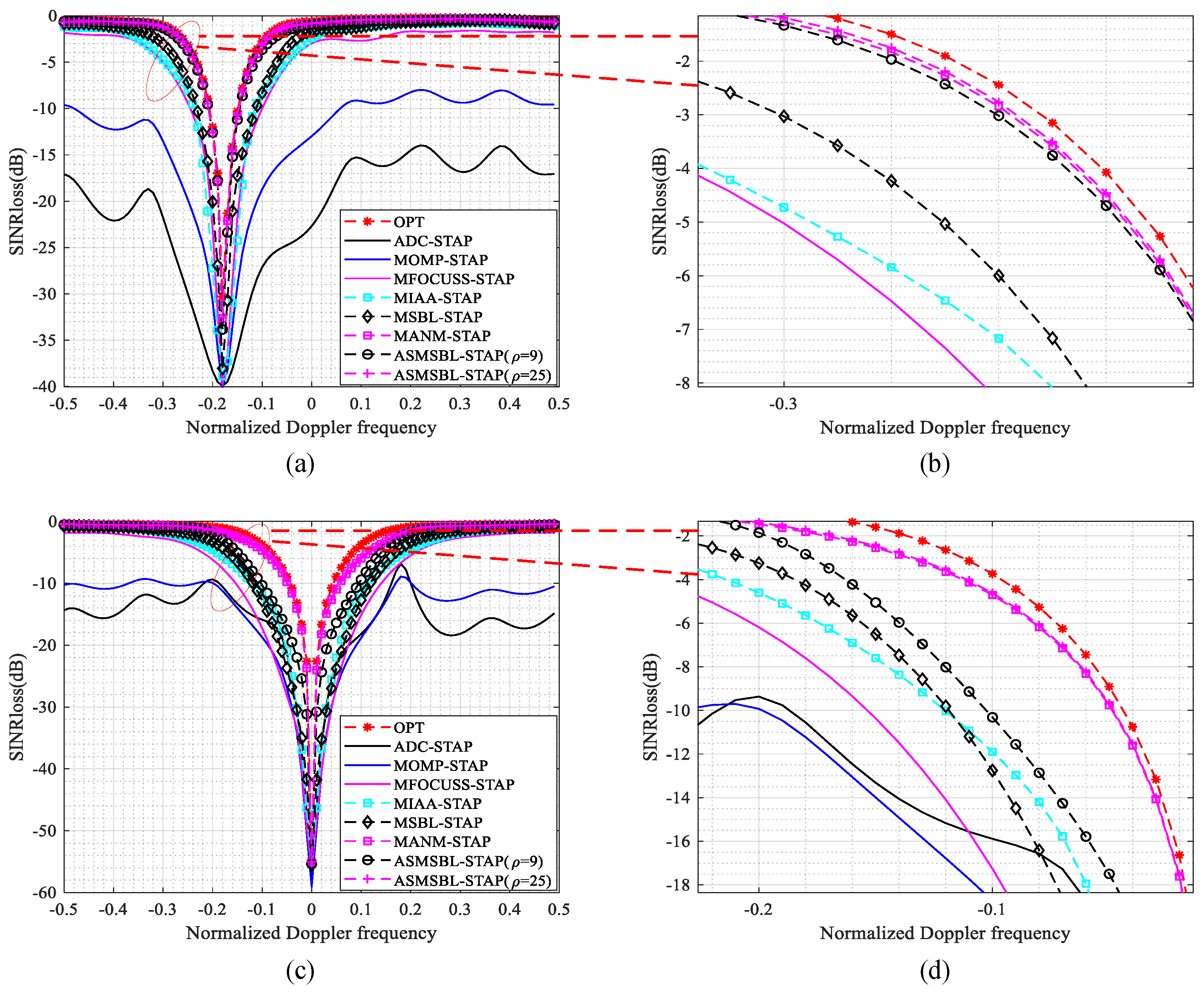
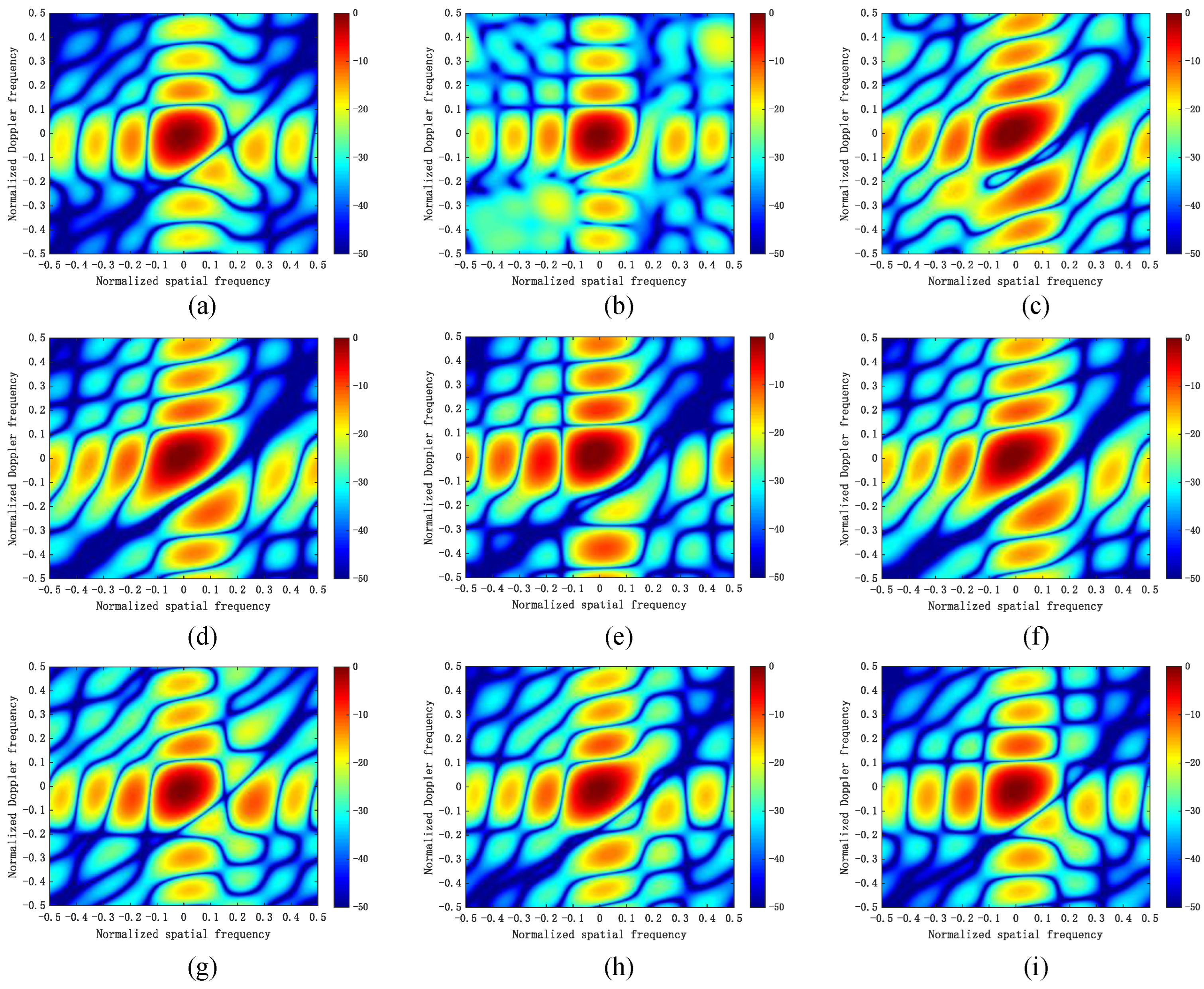
5. Numerical Simulation

In this section, the performance of the proposed ASMSBL-STAP algorithm is validated through simulation experiments, and performance comparisons are made with the traditional ADC-STAP [23], MOMP-STAP [40], MFOCUSS-STAP [41], MIAA-STAP [42], MSBL-STAP [49] and MANM-STAP [43] algorithms. In airborne bistatic radar scenarios, although there exists a serious grid mismatch problem, the MANM-STAP algorithm can achieve a close to optimal clutter suppression performance. If the proposed ASMSBL-STAP algorithm can achieve a performance close to or slightly better than the MANM-STAP algorithm, it proves that the proposed algorithm can achieve near-optimal performance. The performance of some recently proposed Bayesian framework-based gridless SR STAP algorithms [55,56] is slightly better than the MANM-STAP algorithm, but their computational complexity is much greater than the MANM-STAP algorithm. Therefore, in the following experimental section, we chose the MANM-STAP algorithm as a representative of the gridless SR STAP algorithms to compare with the proposed ASMSBL-STAP algorithm. This will easily illustrate the superior clutter suppression performance and high computational efficiency of the proposed ASMSBL-STAP algorithm. In the simulation experiments, the radar carried by both the transmitting platform and the receiving platform is a pulse Doppler radar with a side-looking ULA. The detailed airborne bistatic radar system parameters are given in Table 2. The distance cell under test (CUT) is the 1000th range cell. In all SR STAP algorithms, the number of training samples utilized is 10. The prior parameters are set as c = d = 0 . In the simulation, in the traditional SR STAP algorithms, we set ρ s = 5 and ρ d = 5 . In the proposed ASMSBL-STAP algorithm, we encrypted the grid to solve the grid mismatch problem. We set ρ s = 5 ρ and ρ d = 5 ρ , where ρ = 9 ,   25 , indicating that we have, respectively, encrypted the grid by 9 times and 25 times. All simulation results are averaged over 100 Monte Carlo trials. We evaluate the clutter suppression capability of the all STAP algorithms using the signal-to-interference-plus-noise ratio (SINR) loss, represented by
SIN R loss = σ 2 N K w opt H s t w opt H R i d e a l w opt
where R i d e a l represents the exact CNCM.
In Figure 4, we compared the convergence performance of various SR STAP algorithms. The cost function C = ln R c + n + Tr R c + n 1 R i d e a l [62] is used as the evaluation indicator of the convergence performance. From Figure 4, we can observe that the convergence speed of the proposed ASMSBL-STAP is significantly faster than the traditional MSBL-STAP algorithm. The reason is that, in the iteration process of the MSBL algorithm, we iteratively select the atoms that contribute the most and then use these selected atoms for sparse recovery in the clutter subspace. This avoids using many redundant atoms in the space-time dictionary and accelerates the convergence speed. Comparing the convergence curves under the conditions of ρ = 9 and ρ = 25 , it can also be observed that, in the proposed ASMSBL-STAP algorithm, when we use an encrypted grid to solve the grid mismatch problem, the convergence speed of the algorithm will slow down accordingly. The reason for this is that when the grid becomes finer, we need to select more atoms to construct the clutter support subspace more accurately. Even though the convergence speed of the proposed ASMSBL-STAP algorithm is not as fast as that of the MOMP-STAP algorithm and the MFOCUSS-STAP algorithm, both of these two algorithms cannot solve the grid mismatch problem. Thus, in the bistatic airborne radar scenario, their sparse recovery performance is poor.
In Table 3, a comparison is provided of the average running time of the different STAP algorithms. The data were acquired using MATLAB 2018b on a computer featuring an Intel(R) Xeon(R) E5-2620 CPU clocked at 2.40 GHz. Based on the results shown in Figure 3, we have established the number of iterations for the following algorithms: MFOCUSS-STAP (50 iterations), MIAA-STAP (20 iterations) and MSBL-STAP (200 iterations). From Table 3, we can observe that the traditional statistical ADC-STAP algorithm and traditional SR STAP algorithms, such as MOMP-STAP, MFCOUSS-STAP and MIAA-STAP, have higher efficiency. But they face an insufficient sample size problem or a grid mismatch problem and have limited clutter suppression capability in the bistatic airborne radar scenario. Compared to the MSBL-STAP algorithm, our proposed ASMSBL-STAP algorithm not only solves the grid mismatch problem but also has a higher efficiency. Although the MANM-STAP method can effectively solve the problem of grid mismatch, the algorithm’s average running time is long because the CVX solver is required during the solving process. Comparing the average running time under the conditions of ρ = 9 and ρ = 25 , we know that, in our proposed ASMSBL-STAP algorithm, the cost of using encrypted grids to solve the grid mismatch problem is a decrease in efficiency.
The clutter suppression capability of the STAP algorithms is contingent on the accurate estimation of the CNCM, and the estimation accuracy of the CNCM is reflected in the clutter Capon spectrum. Thus, next, in Figure 5, we present the clutter Capon spectra of the ADC-STAP algorithm, MSBL-STAP algorithm, MANM-STAP algorithm and the proposed ASMSBL-STAP algorithm in four different airborne bistatic radar scenarios to demonstrate the superior clutter suppression capability of our algorithm. For comparison, we also provide the ideal clutter Capon spectra in four different airborne bistatic radar scenarios. These four airborne bistatic radar scenarios are, respectively, a transmitter and receiver on a collinear flight path, a transmitter and receiver on a parallel flight path, a transmitter and receiver on a vertical flight path and a transmitter and receiver on a crossing flight path. In the proposed ASMSBL-STAP algorithm, we set ρ = 25 . From Figure 5, we can observe that the traditional ADC-STAP algorithm cannot estimate the CNCM accurately and has a poor clutter suppression effect when the training samples are inadequate. Comparing the ideal clutter Capon spectra and the clutter Capon spectra of the MSBL-STAP algorithm in four different scenarios, we find that the traditional MSBL-STAP algorithm cannot estimate the CNCM well in the airborne bistatic radar scenario due to the influence of grid mismatch, so its clutter suppression capability is greatly reduced. Comparing the ideal clutter Capon spectra and the clutter Capon spectra of the MANM-STAP algorithm and the proposed ASMSBL-STAP algorithm in four different scenarios, we know that, in the case of grid mismatch, both the MANM-STAP and the proposed ASMSBL-STAP algorithm can effectively estimate the clutter Capon spectrum. However, compared to the MANM-STAP algorithm, our proposed ASMABL-STAP algorithm is much more efficient.
In Figure 6, we plot the SINR loss curves of different STAP algorithms under two airborne bistatic radar scenarios. Figure 6a plots the SINR loss curves of different STAP algorithms under the scenario of a transmitter and receiver on a collinear flight path. Figure 6b plots the detailed enlargement of Figure 6a. Figure 6c plots the SINR loss curves of different STAP algorithms under the case of a transmitter and receiver on a parallel flight path. Figure 6d plots the detailed enlargement of Figure 6c. In the proposed ASMSBL-STAP algorithm, we plot the SINR loss curves under the conditions of ρ = 9 and ρ = 25 . For comparison, we also provide the optimal SINR loss curves for two different airborne bistatic radar scenarios. From Figure 6, we can observe that the SINR loss curves of the MANM-STAP algorithm and the proposed ASMSBL-STAP algorithm ( ρ = 25 ) are closest to the ideal SINR loss curve, meaning they can achieve a close to optimal clutter suppression performance. Comparing the SINR loss curves of the MSBL-STAP algorithms and proposed ASMSBL-STAP under the conditions ρ = 9 and ρ = 25 , we find that the notch width of the SINR loss curve of the proposed ASMSBL-STAP algorithm ( ρ = 9 ) is smaller than that of the traditional MSBL-STAP algorithm but larger than that of the ASMSBL-STAP algorithm ( ρ = 25 ). This indicates that when ρ = 9 , due to grid refinement, the proposed ASMSBL-STAP algorithm partially alleviates the adverse effects of grid mismatch on clutter suppression. And as the grid becomes denser, such as when ρ = 25 , it can be seen that our algorithm has effectively alleviated the grid mismatch problem, thereby achieving a SINR loss curve close to optimal. This demonstrates the superior clutter suppression ability of the proposed algorithm in the airborne bistatic radar scenario. From Figure 6, we can also observe that, in the scenario of airborne bistatic radars, due to the limitations of the number of training samples and the impact of grid mismatch, the SINR loss curve of other STAP algorithms has wide notches, indicating their poor clutter suppression capability.
To provide a more intuitive comparison of the clutter suppression capabilities of various STAP algorithms, in Figure 7 we plot the two-dimensional adaptive patterns of various STAP algorithms in the scenario of a transmitter and receiver on a collinear flight path. For the proposed ASMSBL-STAP algorithm, we plotted the two-dimensional adaptive patterns under the conditions of ρ = 9 and ρ = 25 . For comparison, the optimal two-dimensional adaptive pattern using the ideal CNCM is provided. From Figure 7, we can observe that the MANM-STAP algorithm and the proposed ASMSBL-STAP algorithm ( ρ = 25 ) are able to form notches well on clutter ridges, and the two-dimensional adaptive direction diagrams they form are closest to the optimal. This further illustrates the superior clutter suppression capability of our proposed algorithm. Comparing the two-dimensional adaptive patterns of the MSBL-STAP algorithm and the OPT, we find that, due to the influence of grid mismatch, the notch formed by the MSBL-STAP algorithm on the clutter ridge is wide, which may lead to slow-moving targets also being suppressed. Comparing the two-dimensional adaptive patterns of the proposed ASMSBL-STAP algorithm under the conditions ρ = 9 and ρ = 25 , we know that as the grid continues to be encrypted, the two-dimensional adaptive pattern of the proposed ASMSBL-STAP algorithm becomes closer and closer to the optimal. Due to the limitations in the number of training samples and the impact of grid mismatch, other STAP algorithms cannot form good two-dimensional adaptive patterns, so they have a limited ability to suppress clutter in the airborne bistatic radar scenario.
In Figure 8, to more intuitively illustrate the clutter suppression ability of the proposed ASMSBL-STAP algorithm, we plot time-domain adaptive patterns sliced along the main lobe direction of the different SR STAP algorithms in Figure 7, as well as a local enlargement map. The normalized spatial frequency and the normalized Doppler frequency in the main lobe direction are 0 and −0.033, respectively. From Figure 8a,b, we know that, due to its inability to resolve the grid mismatch problem in the airborne bistatic radars, the MSBL-STAP algorithm formed a notch at f d = 0.181 , while the actual clutter notch position is at f d = 0.178 ; there is a deviation between the clutter notch position formed by the MSBL-STAP algorithm and the actual clutter notch position. When ρ = 9 , the proposed ASMSBL-STAP algorithm formed a notch at the position f d = 0.179 ; compared with the MSBL-STAP algorithm, the clutter notch formed by the proposed ASMSBL-STAP algorithm is more accurate, and the reason for this is that the grid mismatch problem was alleviated after grid refinement. The MANM-STAP algorithm and the proposed ASMSBL-STAP algorithm ( ρ = 25 ), since they have effectively solved the grid mismatch problem, both formed notches at the actual clutter notch position of f d = 0.178 . This indicates that these two algorithms are capable of precisely forming notches at the clutter location while protecting the target. From Figure 8b, by comparing the notch depth formed by various SR STAP algorithms, we also know that, compared to the MSBL-STAP algorithm and the MANM-STAP algorithm, the proposed ASMSBL-STAP algorithm ( ρ = 25 ) can form a deeper and more accurate clutter notch, which verifies the superior clutter suppression capability of the proposed algorithm.
In Figure 9, we plot the curves of the average SINR loss versus the number of training samples for various STAP algorithms. From Figure 9, we can observe that the average SINR loss decreases as the number of training samples increases across all STAP algorithms. We also find that when the number of training samples is greater than 10, the average SINR loss of the MAMN-STAP and the proposed ASMSBL-STAP algorithm ( ρ = 25 ) can approach the optimum and that the average SINR losses of the proposed ASMSBL-STAP algorithm ( ρ = 9 ) and the MIAA-STAP algorithm are relatively close to the optimum. As for the other SR STAP algorithms, due to the influence of grid mismatch, even with an increase in the number of training samples, their average SINR loss cannot approach the optimum.
Detection probability (PD) is employed as a visual evaluation metric to assess the effectiveness of the proposed ASMSBL-STAP algorithm at target detection. Simulation experiments are conducted utilizing an adaptive matched filter detector (AMF) [63]. In total, 100/PFA samples are utilized for determining the detection threshold, and 1000 Monte Carlo experiments are conducted to calculate the PD [14,15,16,64]. In Figure 10, we plot the fluctuation curves of the PD across different STAP algorithms as the target SNR varies within the scenario of a transmitter and receiver on a collinear flight path, given a false alarm probability (PFA) of 10 3 . In the proposed ASMSBL-STAP algorithm, we plot the PD versus SNR curves under the conditions ρ = 9 and ρ = 25 . For comparison, we also provide the optimal PD versus SNR curves. Figure 10a,b plot the PD versus SNR curves of various STAP algorithms under the conditions of f d t = 0.1 and f d t = 0.2 , which are used to measure the target detection capability of different STAP algorithms in the main lobe clutter region and the sidelobe clutter region. From Figure 10, it is evident that the proposed ASMSBL-STAP algorithm ( ρ = 25 ) and the MANM-STAP algorithm demonstrate nearly optimal target detection performances within both the main lobe clutter area ( f d t = 0.1 ) and the sidelobe clutter area ( f d t = 0.2 ). In Figure 10a, the influence of grid mismatch is evident, leading to a limitation in the performance of the conventional SR STAP algorithms, including MOMP-STAP, MFCOUSS-STAP, MIAA-STAP and MSBL-STAP, in achieving optimal target detection in the main lobe clutter region ( f d t = 0.1 ). This deficiency highlights their limited capability to detect slow-moving targets. We can also observe that, whether in the main lobe clutter region ( f d t = 0.1 ) or in the sidelobe clutter region ( f d t = 0.2 ), due to the limited number of training samples, traditional ADC-STAP cannot achieve a good target detection performance. Comparing the PD versus SNR curves of the proposed ASMSBL-STAP algorithm under the conditions ρ = 9 and ρ = 25 , we find that grid encryption alleviates the adverse effects caused by grid mismatch and that as the grid becomes denser, the target detection performance of the proposed ASMSBL-STAP algorithm also improves accordingly.
We use the receiver operating characteristic (ROC) curves to visually demonstrate the relationship between the PD and PFA. In Figure 11, we depict the ROC curves for slow-moving targets characterized by f d t = 0.1 and fast-moving targets characterized by f d t = 0.2 in the scenario of a transmitter and receiver on a collinear flight path. The SNR conditions under consideration are −8 dB and 2 dB. In the proposed ASMSBL-STAP algorithm, we plot the ROC curves under the conditions ρ = 9 and ρ = 25 . For comparison, the optimal ROC curves are also provided. Comparing Figure 11a,c and Figure 11b,d, we find that with the increase in the SNR, the PD of all STAP algorithms increases accordingly. Similarly, as shown in Figure 11, we can observe that both the proposed ASMSBL-STAP algorithm ( ρ = 25 ) and the MANM-STAP algorithm have ROC curves that can approximate the optimal curve. However, compared to the MANM-STAP algorithm, the proposed ASMSBL-STAP algorithm is much more efficient. Comparing the ROC curves of the MSBL-STAP algorithm and the proposed ASMSBL-STAP algorithm under the conditions ρ = 9 and ρ = 25 , we find that the proposed ASMSBL-STAP algorithm can solve the grid mismatch problem in the airborne bistatic radar scenario, and thus can achieve a better target detection performance. Moreover, as the grid becomes denser, the grid mismatch problem is being solved more effectively, leading to improved the target detection performance of the proposed ASMSBL-STAP algorithm. From Figure 11, we also find that other STAP algorithms, such as ADC-STAP, MOMP-STAP, MIAA-STAP and MFOCUSS-STAP, are affected by the limited number of training samples or grid mismatch and cannot achieve good target detection performance.

6. Conclusions

In this article, we proposed an SR STAP algorithm for airborne bistatic radars based on atomic selection under the Bayesian framework. The proposed algorithm iteratively selected the atoms that contributed the most to the signal model and used these selected atoms to estimate the clutter support subspace and perform sparse recovery in the clutter support subspace. Due to the inherent sparsity of clutter, performing a sparse recovery of clutter signals in the clutter support subspace is much faster than that using an overcomplete space-time dictionary matrix, which indicated that the proposed ASMSBL-STAP algorithm is a highly efficient algorithm. When there existed a grid mismatch problem in the airborne bistatic radar scenario, the proposed algorithm obtained a finer space-time dictionary matrix by encrypting grid points, making the selected atoms closer to the clutter ridge, thereby alleviating the adverse effects of grid mismatch. Since the proposed algorithm performed sparse recovery in the clutter support subspace, encrypting the grid points did not impose a significant computational burden. Moreover, the proposed ASMSBL-STAP algorithm integrated out the noise term under a new hierarchical Bayesian model to mitigate the negative impact resulting from imprecise noise power estimation in the iterative process of the conventional MSBL-STAP algorithm, which further enhanced its performance. We analyzed the efficiency and proved the convergence of the proposed ASMSBL-STAP algorithm. Finally, the simulation results demonstrated that the proposed ASMSBL-STAP algorithm has a superior clutter suppression performance and target detection performance in the airborne bistatic radar scenario.

Author Contributions

Conceptualization, K.L. and T.W.; investigation, K.L.; methodology, K.L. and W.H.; project administration, T.W.; software, K.L.; supervision, W.H.; visualization, K.L.; writing—original draft, K.L.; writing—review and editing, K.L. All authors have read and agreed to the published version of the manuscript.

Funding

This research was funded by National Key R&D Program of China, grant number 2021YFA1000400.

Data Availability Statement

The raw data supporting the conclusions of this article will be made available by the authors on reasonable request.

Conflicts of Interest

The authors declare no conflicts of interest.

Appendix A

This appendix contains formulas for quickly updating the variables h j ,   p j , l ,   q j , l , μ l , Σ , j . To simplify the formulas, the variables with the ~ represent the current iteration, while variables without the ~ represent the variables from the last iteration.
(1) If ξ i t = 0 and ξ i t + 1 > 0 , add ξ i t + 1 to η t and add d i to Φ t , i.e., η t + 1 = η t ; ξ i t + 1 , Φ t + 1 = Φ t , d i .
2 Δ T ξ j = log α j α j + h j 2 N K + 2 c log 1 p j , l 2 / q j , l α j + h j
Σ ˜ = Σ + τ Σ Φ T d j d j T Φ Σ τ Σ Φ T d j τ Σ Φ T d j T τ
μ ˜ l = μ l δ Σ Φ T d j δ
H ˜ j = H j τ d j T e j 2 , j = 1 , 2 , , 2 N s K d
P ˜ j , l = P j , l δ d j T e j , j = 1 , 2 , , 2 N s K d
Q ˜ j , l = Q j , l τ z l T d j 2 , j = 1 , 2 , , 2 N s K d
where α j = ξ j 1 , τ = α j + H j 1 , δ = τ P j , l and e j = d j Φ Σ Φ T d j .
(2) If ξ i t > 0 and ξ i t + 1 > 0 , update ξ i in η t , Φ t + 1 = Φ t .
2 Δ T ξ j = 2 N K + 2 c 1 log 1 + H j α ˜ j 1 α j 1 + 2 N K + 2 c log α j + h j q j , l p j , l 2 α ˜ j α ˜ j + h j q j , l p j , l 2 α j
Σ ˜ = Σ ς j Σ k Σ k T
μ ˜ l = μ l ς j δ Σ k
H ˜ j = H j + ς j Σ k T Φ T d j T 2 , j = 1 , 2 , , 2 N s K d
P ˜ j , l = P j , l + ς j δ Σ k T Φ T d j T , j = 1 , 2 , , 2 N s K d
Q ˜ j , l = Q j , l + ς j Σ k T Φ T z l 2 , j = 1 , 2 , , 2 N s K d
where α ˜ j = ξ ˜ j 1 , ς j = τ + α ˜ j α j 1 1 and Σ k is the k th , k = 1 , 2 , , M column of Σ .
(3) If ξ i t > 0 and ξ i t + 1 = 0 , remove ξ i in η t and remove d i in Φ t .
2 Δ T ξ j = 2 N K + 2 c log 1 + P j , l 2 / Q j , l α j H j log 1 H j α j
Σ ˜ = Σ 1 τ Σ k Σ k T
μ ˜ l = μ l δ τ Σ k
H ˜ j = H j + 1 τ Σ k T Φ T d j T 2 , j = 1 , 2 , , 2 N s K d
P ˜ j , l = P j , l + δ τ Σ k T Φ T d j T , j = 1 , 2 , , 2 N s K d
Q ˜ j , l = Q j , l + 1 τ Σ k T Φ T z l 2 , j = 1 , 2 , , 2 N s K d
It is important to note that we should remove the Σ k and μ k corresponding to the atom that needs to be removed when updating (A14) and (A15).

References

  1. Klemm, R. Comparison between monostatic and bistatic antenna configurations for STAP. IEEE Trans. Aerosp. Electron. Syst. 2000, 36, 596–608. [Google Scholar] [CrossRef]
  2. Himed, B.; James, H.M.; Zhang, Y.H. Bistatic STAP performance analysis in radar applications. In Proceedings of the 2001 IEEE Radar Conference, Atlanta, GA, USA, 3 May 2001; pp. 198–203. [Google Scholar]
  3. Gelli, S.; Bacci, A.; Martorella, M.; Berizzi, F. Clutter suppression and high-resolution imaging of noncooperative ground targets for bistatic airborne radar. IEEE Trans. Aerosp. Electron. Syst. 2017, 54, 932–949. [Google Scholar] [CrossRef]
  4. Klemm, R. Effect of bistatic radar configurations on STAP. In Proceedings of the European Synthetic Aperture Radar Conference, Munich, Germany, 23–25 May 2000; pp. 817–820. [Google Scholar]
  5. Duan, R.; Wang, X.; Chen, Z. Space-time clutter model for airborne bistatic radar with non-Gaussian statistics. In Proceedings of the 2008 IEEE Radar Conference, Adelaide, SA, Australia, 2–5 September 2008; pp. 1–6. [Google Scholar]
  6. Reed, I.S.; Mallett, J.D.; Brennan, L.E. Rapid convergence rate in adaptive arrays. IEEE Trans. Aerosp. Electron. Syst. 1974, 10, 853–863. [Google Scholar] [CrossRef]
  7. Klemm, R. Principles of Space-Time Adaptive Processing; The Institution of Electrical Engineers: London, UK, 2002. [Google Scholar]
  8. Brennan, L.E.; Mallett, J.D.; Reed, I.S. Theory of adaptive radar. IEEE Trans. Aerosp. Electron. Syst. 1973, 9, 237–251. [Google Scholar] [CrossRef]
  9. Melvin, W.L. Space-time adaptive radar performance in heterogeneous clutter. IEEE Trans. Aerosp. Electron. Syst. 2000, 36, 621–633. [Google Scholar] [CrossRef]
  10. DiPietro, R. Extended factored space–time processing for airborne radar systems. Signals Syst. Comput. 1992, 1, 425–430. [Google Scholar]
  11. Song, D.; Feng, Q.; Chen, S.; Xi, F.; Liu, Z. Space-time adaptive processing using deep neural network-based shrinkage algorithm under small training samples. IEEE Trans. Aerosp. Electron. Syst. 2023, 59, 9697–9703. [Google Scholar] [CrossRef]
  12. Klintberg, J.; McKelvey, T.; Dammert, P. A parametric approach to space-time adaptive processing in bistatic radar systems. IEEE Trans. Aerosp. Electron. Syst. 2021, 58, 1149–1160. [Google Scholar] [CrossRef]
  13. Song, D.; Feng, Q.; Chen, S.; Xi, F.; Liu, Z. Random matrix theory-based reduced-dimension space-time adaptive processing under finite training samples. Remote Sens. 2022, 14, 3959. [Google Scholar] [CrossRef]
  14. Liu, W.J.; Xie, W.C.; Liu, J.; Wang, Y. Adaptive double subspace signal detection in Gaussian background-Part I: Homogeneous environments. IEEE Trans. Signal Process. 2014, 62, 2345–2357. [Google Scholar] [CrossRef]
  15. Liu, W.J.; Liu, J.; Gao, Y.C.; Wang, G.; Wang, Y.-L. Multichannel signal detection in interference and noise when signal mismatch happens. Signal Process. 2020, 166, 107268. [Google Scholar] [CrossRef]
  16. Liu, W.J.; Liu, J.; Du, Q.L.; Wang, Y.-L. Distributed target detection in partially homogeneous environment when signal mismatch occurs. IEEE Trans. Signal Process. 2018, 66, 3918–3928. [Google Scholar] [CrossRef]
  17. Meng, Z.; Shen, F. Robust space-time adaptive processing method for GNSS receivers in coherent signal environments. Remote Sens. 2023, 15, 4212. [Google Scholar] [CrossRef]
  18. Huang, P.; Zou, Z.; Xia, X.G.; Liu, X.; Liao, G. A novel dimension-reduced space-time adaptive processing algorithm for spaceborne multichannel surveillance radar systems based on spatial–temporal 2-D sliding window. IEEE Geosci. Remote Sens. 2022, 60, 1–21. [Google Scholar] [CrossRef]
  19. Ward, J.; Steinhardt, A.O. Multiwindow post-Doppler space-time adaptive processing. In Proceedings of the IEEE Signal Processing Workshop Statistical Signal Array Processing, Quebec, QC, Canada, 26–29 June 1994. [Google Scholar]
  20. Ward, J. Space-Time Adaptive Processing for Airborne Radar; MIT Lincoln Laboratory: Lexington, KY, USA, 1994. [Google Scholar]
  21. Borsari, G.K. Mitigating effects on STAP processing caused by an inclined array. In Proceedings of the 1998 IEEE Radar Conference, Dallas, TX, USA, 14 May 1998; pp. 135–140. [Google Scholar]
  22. Zhao, H.; Shi, Y.; Zhang, B.; Shi, M. Analysis and simulation of interference suppression for space-time adaptive processing. In Proceedings of the IEEE International Conference on Signal Processing, Communications and Computing, Guilin, China, 5–8 August 2014; pp. 724–727. [Google Scholar]
  23. Himed, B.; Zhang, Y.; Hajjari, A. STAP with angle-Doppler compensation for bistatic airborne radars. In Proceedings of the 2002 IEEE Radar Conference, Long Beach, CA, USA, 25 April 2002; pp. 311–317. [Google Scholar]
  24. Melvin, W.L.; Davis, M.E. Adaptive cancellation method for geometry-induced nonstationary bistatic clutter environments. IEEE Trans. Aerosp. Electron. Syst. 2007, 43, 651–672. [Google Scholar] [CrossRef]
  25. Shen, M.; Yu, J.; Wu, D.; Zhu, D. An efficient adaptive angle-Doppler compensation approach for non-sidelooking airborne radar STAP. Sensors 2015, 15, 13121–13131. [Google Scholar] [CrossRef] [PubMed]
  26. Lapierre, F.D.; Verly, J.G.; Van Droogenbroeck, M. New solutions to the problem of range dependence in bistatic STAP radars. In Proceedings of the 2003 IEEE Radar Conference, Huntsville, AL, USA, 8 May 2003; pp. 452–459. [Google Scholar]
  27. Varadarajan, V.; Krolik, J.L. Space-time interpolation for adaptive arrays with limited training data. In Proceedings of the 2003 IEEE International Conference on Acoustics, Speech, and Signal Processing, Hong Kong, China, 6–10 April 2003; pp. V–353. [Google Scholar]
  28. Varadarajan, V.; Krolik, J.L. Joint space-time interpolation for bistatic STAP. In Proceedings of the Thrity-Seventh Asilomar Conference on Signals, Systems & Computers, Pacific Grove, CA, USA, 9–12 November 2003; pp. 60–65. [Google Scholar]
  29. Zatman, M. Performance analysis of the derivative based updating method. In Proceedings of the Adaptive Sensor Array Processing Workshop, MIT Lincoln Lab., Lexington, MA, USA, 13–14 March 2001. [Google Scholar]
  30. Baraniuk, R.G. Compressive sensing. IEEE Signal Proc. Mag. 2007, 24, 118–121. [Google Scholar] [CrossRef]
  31. Trzasko, J.; Manduca, A. Relaxed conditions for sparse signal recovery with general concave priors. IEEE Trans. Signal Process. 2009, 57, 4347–4354. [Google Scholar] [CrossRef]
  32. Mallat, S.G.; Zhang, Z. Matching pursuits with time-frequency dictionaries. IEEE Trans. Signal Process. 1993, 41, 3397–3415. [Google Scholar] [CrossRef]
  33. Tropp, J.A.; Gilbert, A.C. Signal recovery from random measurements via orthogonal matching pursuit. IEEE Trans. Inf. Theory 2007, 53, 4655–4666. [Google Scholar] [CrossRef]
  34. Koh, K.; Kim, S.J.; Boyd, S. An interior-point method for large-scale ℓ1-regularized logistic regression. J. Mach. Learn. Res. 2007, 1, 606–617. [Google Scholar]
  35. Gorodnitsky, I.F.; Rao, B.D. Sparse signal reconstruction from limited data using FOCUSS: A re-weighted minimum norm algorithm. IEEE Trans. Signal Process. 1997, 45, 600–616. [Google Scholar] [CrossRef]
  36. Yardibi, T.; Li, J.; Stoica, P.; Xue, M.; Baggeroer, A.B. Source localization and sensing: A nonparametric iterative adaptive approach based on weighted least squares. IEEE Trans. Aerosp. Electron. Syst. 2010, 46, 425–443. [Google Scholar] [CrossRef]
  37. Yang, Z.C.; Li, X.; Wang, H.Q.; Jiang, W.D. On clutter sparsity analysis in space-time adaptive processing airborne radar. IEEE Geosci. Remote Sens. Lett. 2013, 10, 1214–1218. [Google Scholar] [CrossRef]
  38. Zhang, S.; Wang, T.; Liu, C.; Ren, B. A fast IAA−based SR−STAP method for airborne radar. Remote Sens. 2024, 16, 1388. [Google Scholar] [CrossRef]
  39. Li, X.; Yang, X.; Wang, Y.; Duan, K. Gridless sparse clutter nulling STAP based on particle swarm optimization. IEEE Geosci. Remote Sens. Lett. 2022, 19, 1–5. [Google Scholar] [CrossRef]
  40. Ślesicka, A.; Kawalec, A. An application of the orthogonal matching pursuit algorithm in space-time adaptive processing. Sensors 2020, 20, 3468. [Google Scholar] [CrossRef]
  41. Yang, X.; Sun, Y.; Zeng, T.; Long, T. Iterative roubust sparse recoery method based on focuss for space-time adaptive processing. In Proceedings of the IET International Radar Conference, Hangzhou, China, 14–16 October 2015; pp. 1–6. [Google Scholar]
  42. Yang, Z.C.; Li, X.; Wang, H.; Jiang, W. Adaptive clutter suppression based on iterative adaptive approach for airborne radar. Signal Process. 2013, 93, 3567–3577. [Google Scholar] [CrossRef]
  43. Feng, W.; Guo, Y.; Zhang, Y.; Gong, J. Airborne radar space time adaptive processing based on atomic norm minimization. Signal Process. 2018, 148, 31–40. [Google Scholar] [CrossRef]
  44. Grant, M.; Boyd, S. CVX: Matlab Software for Disciplined Convex Programing, Version 2.0 Beta. Available online: http://cvxr.com/cvx (accessed on 10 April 2024).
  45. Tipping, M.E. Sparse Bayesian learning and the relevance vector machine. J. Mach. Learn. 2001, 1, 211–244. [Google Scholar]
  46. Ji, S.; Xue, Y.; Carin, L. Bayesian compressive sensing. IEEE Trans. Signal Process. 2008, 56, 2346–2356. [Google Scholar] [CrossRef]
  47. Wipf, D.P.; Rao, B.D. Sparse Bayesian learning for basis selection. IEEE Trans. Signal Process. 2004, 52, 2153–2164. [Google Scholar] [CrossRef]
  48. Wipf, D.P.; Rao, B.D. An empirical Bayesian strategy for solving the simultaneous sparse approximation problem. IEEE Trans. Signal Process. 2007, 55, 3704–3716. [Google Scholar] [CrossRef]
  49. Duan, K.Q.; Wang, Z.T.; Xie, W.C.; Chen, H.; Wang, Y.L. Sparsity-based STAP algorithm with multiple measurement vectors via sparse Bayesian learning strategy for airborne radar. IET Signal Process. 2017, 11, 544–553. [Google Scholar] [CrossRef]
  50. Cui, N.; Xing, K.; Yu, Z.; Duan, K. Tensor-based sparse recovery space-time adaptive processing for large size data clutter suppression in airborne radar. IEEE Trans. Aerosp. Electron. Syst. 2022, 59, 907–922. [Google Scholar] [CrossRef]
  51. Liu, C.; Wang, T.; Zhang, S.; Ren, B. Clutter suppression based on iterative reweighted methods with multiple measurement vectors for airborne radar. IET Radar Sonar Navig. 2022, 59, 907–922. [Google Scholar] [CrossRef]
  52. Liu, K.; Wang, T.; Wu, J.; Liu, C.; Cui, W. On the efficient implementation of sparse Bayesian learning-based STAP algorithms. Remote Sens. 2022, 14, 3931. [Google Scholar] [CrossRef]
  53. Wang, D.; Wang, T.; Cui, W.; Zhang, X. A clutter suppression algorithm via enhanced sparse bayesian learning for airborne radar. IEEE Sens. J. 2023, 23, 10900–10911. [Google Scholar] [CrossRef]
  54. Cao, J.; Wang, T.; Wang, D. Beam-space post-Doppler reduced-dimension STAP based on sparse Bayesian learning. Remote Sens. 2024, 16, 307. [Google Scholar] [CrossRef]
  55. Cui, W.; Wang, T.; Wang, D.; Zhang, X. A novel sparse recovery-based space-time adaptive processing algorithm based on gridless sparse Bayesian learning for non-sidelooking airborne radar. IET Radar Sonar Navig. 2023, 17, 1380–1390. [Google Scholar] [CrossRef]
  56. Zhang, X.; Wang, T.; Wang, D. On efficient maximum likelihood algorithm for clutter suppression. IEEE Signal Process. Lett. 2024, 31, 1399–1403. [Google Scholar] [CrossRef]
  57. Dunson, D.B. Empirical Bayes density regression. Stat. Sin. 2007, 17, 481–504. [Google Scholar]
  58. Ji, S.; Dunson, D.; Carin, L. Multitask compressive sensing. IEEE Trans. Signal Process. 2008, 57, 92–106. [Google Scholar] [CrossRef]
  59. Wu, Q.; Zhang, Y.D.; Amin, M.G.; Himed, B. Complex multitask Bayesian compressive sensing. In Proceedings of the 2014 IEEE International Conference on Acoustics, Speech and Signal Processing, Florence, Italy, 4–9 May 2014; pp. 3375–3379. [Google Scholar]
  60. Golub, G.H.; Van Loan, C.F. Matrix Computations; Johns Hopkins Univ. Press: Baltimore, MD, USA, 2013. [Google Scholar]
  61. Wipf, D.P.; Nagarajan, S.S. A New View of Automatic Relevance Determination. In Proceedings of the International Conference on Neural Information Processing Systems, Auckland, New Zealand, 25–28 November 2008; Curran Associates Inc.: Red Hook, NY, USA, 2008; pp. 1–9. [Google Scholar]
  62. Wang, Z.; Xie, W.; Duan, K.; Wang, Y. Clutter suppression algorithm based on fast converging sparse Bayesian learning for airborne radar. Signal Process. 2017, 130, 159–168. [Google Scholar] [CrossRef]
  63. Robey, F.C.; Fuhrmann, D.R.; Kelly, E.J.; Nitzberg, R. A CFAR adaptive matched filter detector. IEEE Trans. Aerosp. Electron. Syst. 1992, 28, 208–216. [Google Scholar] [CrossRef]
  64. Liu, W.J.; Liu, J.; Hao, C.; Gao, Y.; Wang, Y.-L. Multichannel adaptive signal detection: Basic theory and literature review. Sci. China Inf. Sci. 2022, 65, 121301. [Google Scholar] [CrossRef]
Figure 1. Geometry of the airborne bistatic radar system.
Remotesensing 16 02534 g001
Figure 2. Schematic diagram of the grid mismatch phenomenon in two different airborne bistatic radar configurations. (a) Transmitter and receiver on a collinear flight path; (b) Transmitter and receiver on a parallel flight path.
Remotesensing 16 02534 g002
Figure 3. The computational complexity of various SR STAP algorithms as system DOFs change.
Remotesensing 16 02534 g003
Figure 4. Comparison of convergence performance of various SR STAP algorithms.
Remotesensing 16 02534 g004
Figure 5. Clutter Capon spectrums of various STAP algorithms under four airborne bistatic radar scenarios. (a,f,k,p), ideal clutter Capon spectra under four airborne bistatic radar scenarios; (b,g,l,q), clutter Capon spectra of ADC-STAP algorithm under four airborne bistatic radar scenarios; (c,h,m,r), clutter Capon spectra of MSBL-STAP algorithm under four airborne bistatic radar scenarios; (d,i,n,s), clutter Capon spectra of MANM-STAP algorithm under four airborne bistatic radar scenarios; (e,j,o,t), clutter Capon spectra of ASMSBL-STAP algorithm under four airborne bistatic radar scenarios.
Remotesensing 16 02534 g005
Figure 6. SINR loss curves of different STAP algorithms under two airborne bistatic radar scenarios. (a) SINR loss curves of different STAP algorithms under the case of a transmitter and receiver on a collinear flight path; (b) detailed enlargement of (a); (c) SINR loss curves of different STAP algorithms under the case of a transmitter and receiver on a parallel flight path; (d) detailed enlargement of (c).
Remotesensing 16 02534 g006
Figure 7. Two-dimensional adapted patterns of different STAP algorithms. (a) OPT; (b) ADC-STAP; (c) MOMP-STAP; (d) MFOCUSS-STAP; (e) MIAA-STAP; (f) MSBL-STAP; (g) MANM-STAP; (h) ASMSBL-STAP ( ρ = 9 ); (i) ASMSBL-STAP ( ρ = 25 ).
Remotesensing 16 02534 g007
Figure 8. Time-domain adaptive pattern slices along the main lobe direction of the different SR STAP algorithms in Figure 7. (a) Time-domain adaptive pattern slice; (b) detailed enlargement of (a).
Remotesensing 16 02534 g008
Figure 9. The average SINR loss versus the number of training samples.
Remotesensing 16 02534 g009
Figure 10. PD versus SNR curves of various STAP algorithms under transmitter and receiver on collinear flight path. (a) f d t = 0.1 ; (b) f d t = 0.2 .
Remotesensing 16 02534 g010
Figure 11. ROC curves of various STAP algorithms under transmitter and receiver on collinear flight path. (a) f d t = 0.1 ,   SNR = 8 dB ; (b) f d t = 0.1 ,   SNR = 2 dB ; (c) f d t = 0.2 ,   SNR = 8 dB ; (d) f d t = 0.2 ,   SNR = 2 dB .
Remotesensing 16 02534 g011
Table 1. The computational complexities of different SR STAP algorithms.
AlgorithmThe Number of Multiplications in a Single Iteration
MOMP-STAP o N K N s K d L + r s 3 + N K r s 2 + 2 N K r s
MFOCUSS-STAP o N K N s K d L + N K 3 + 2 N K 2 N s K d + N K N s K d 2
MIAA-STAP o N K N s K d L + N K 3 + 4 N K 2 N s K d
MSBL-STAP o N K N s K d L + N K 3 + 3 N K 2 N s K d + 4 N K N s K d 2
MANM-STAP o L 2 + 2 N 1 2 K 1 + N K L 2 L + N K 2.5
ASMSBL-STAP o 8 ρ N K N s K d M + 2 ρ N s K d M 2 + 8 ρ N K M 2 + 2 ρ N K M L
Table 2. Simulation parameters of the airborne bistatic radar system.
ParametersSymbolsValues
BandwidthB2.5 M
Wavelength λ 0.3 m
PRF f r 2000 Hz
Velocity of transmit/receive platform v T / R 150 m/s
Height of transmit/receive platform H T / R 9 km
Number of array element of transmit/receive platform N 8
Pulse number in the CPI of transmit/receive platform K 8
CNRCNR40 dB
Table 3. Average running time of various STAP algorithms.
AlgorithmRunning Time
ADC-STAP0.2886 s
MOMP-STAP0.2717 s
MFOCUSS-STAP4.7805 s
MIAA-STAP1.3196 s
MSBL-STAP77.9928 s
MANM-STAP881.2042 s
ASMSBL-STAP ρ = 9 3.9539 s
ASMSBL-STAP ρ = 25 31.2608 s
Disclaimer/Publisher’s Note: The statements, opinions and data contained in all publications are solely those of the individual author(s) and contributor(s) and not of MDPI and/or the editor(s). MDPI and/or the editor(s) disclaim responsibility for any injury to people or property resulting from any ideas, methods, instructions or products referred to in the content.

