

Robust Landslide Recognition Using UAV Datasets: A Case Study in Baihetan Reservoir
 , ,
, ,
Abstract
:1. Introduction
2. Study Area and Dataset
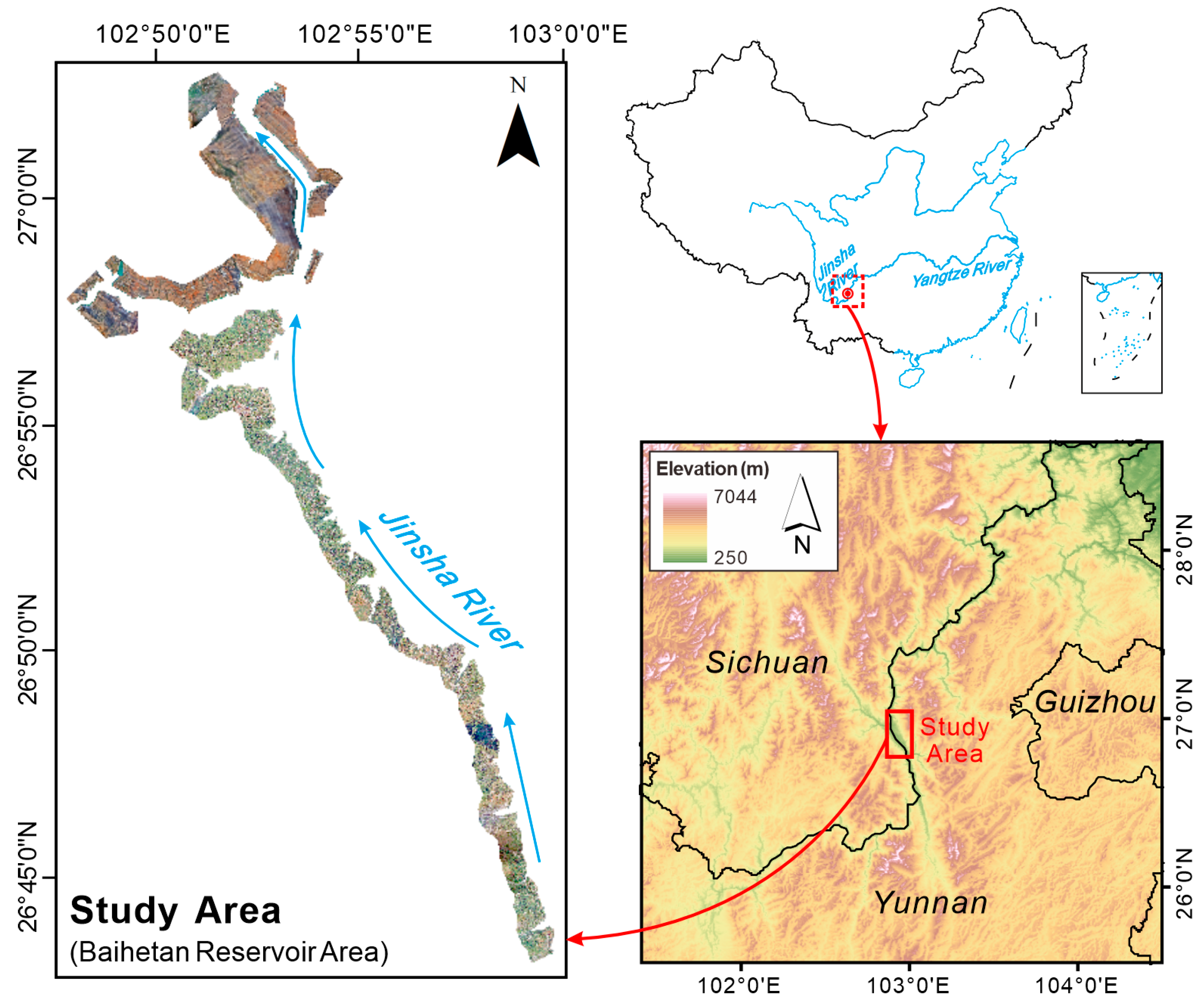
2.1. Study Area and Data Acquisition
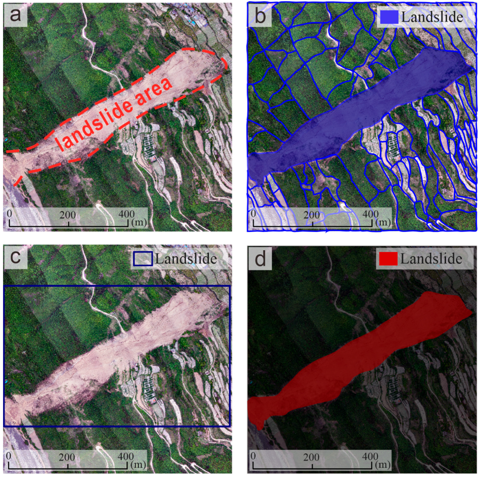
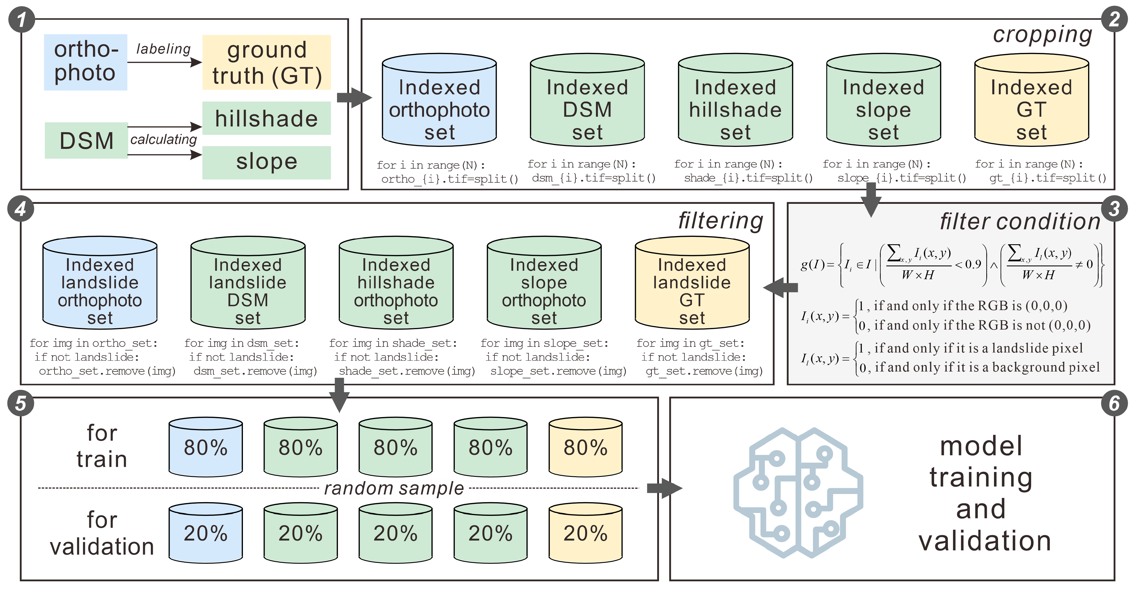
2.2. Dataset Creation
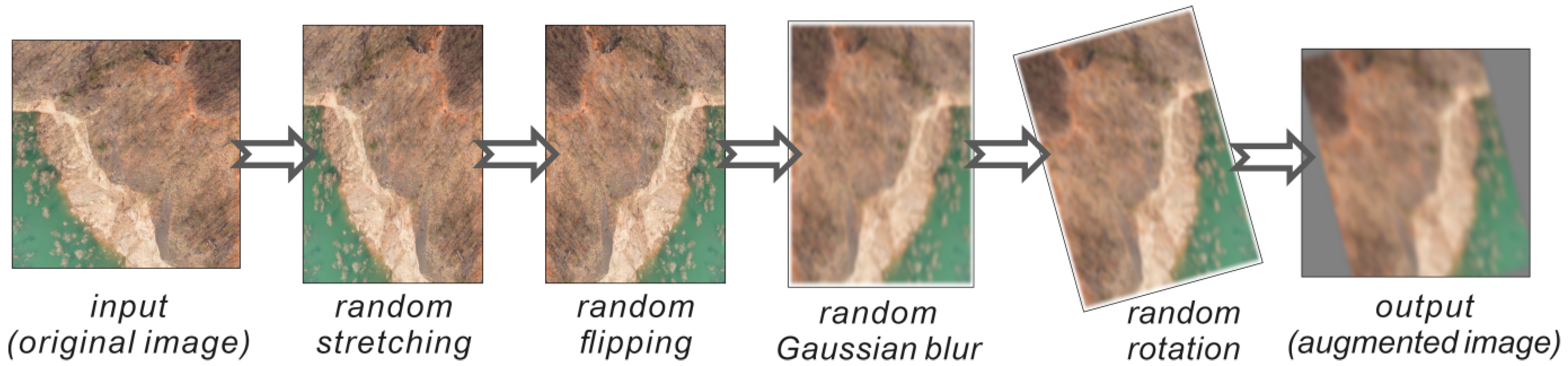
2.3. Dataset Augmentation
3. Methods
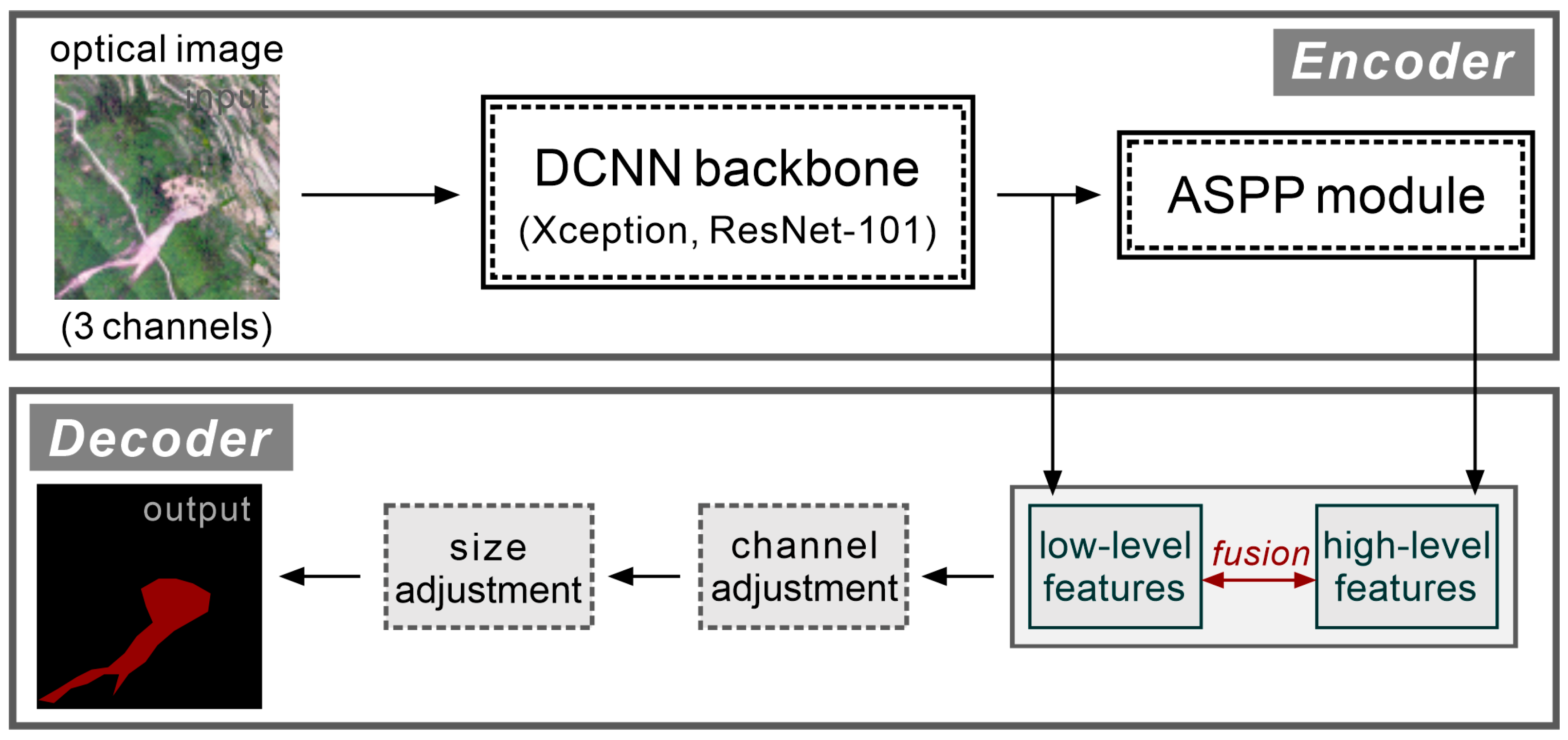
3.1. DeepLabV3+
3.1.1. Model Architecture
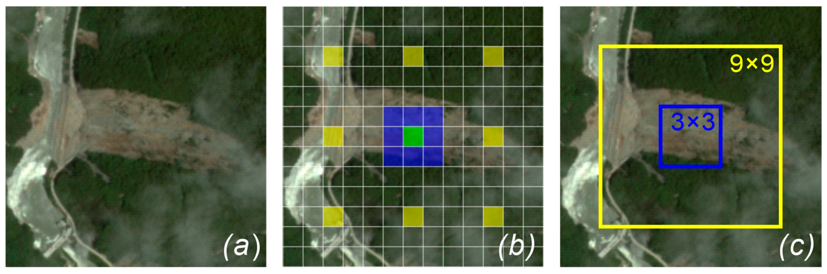
3.1.2. The Dilated Convolution & ASPP Optimizations
3.2. DeepLab4LS: A Dual-Encoder DeepLab Model for Landslide
3.2.1. Basic Design of Model
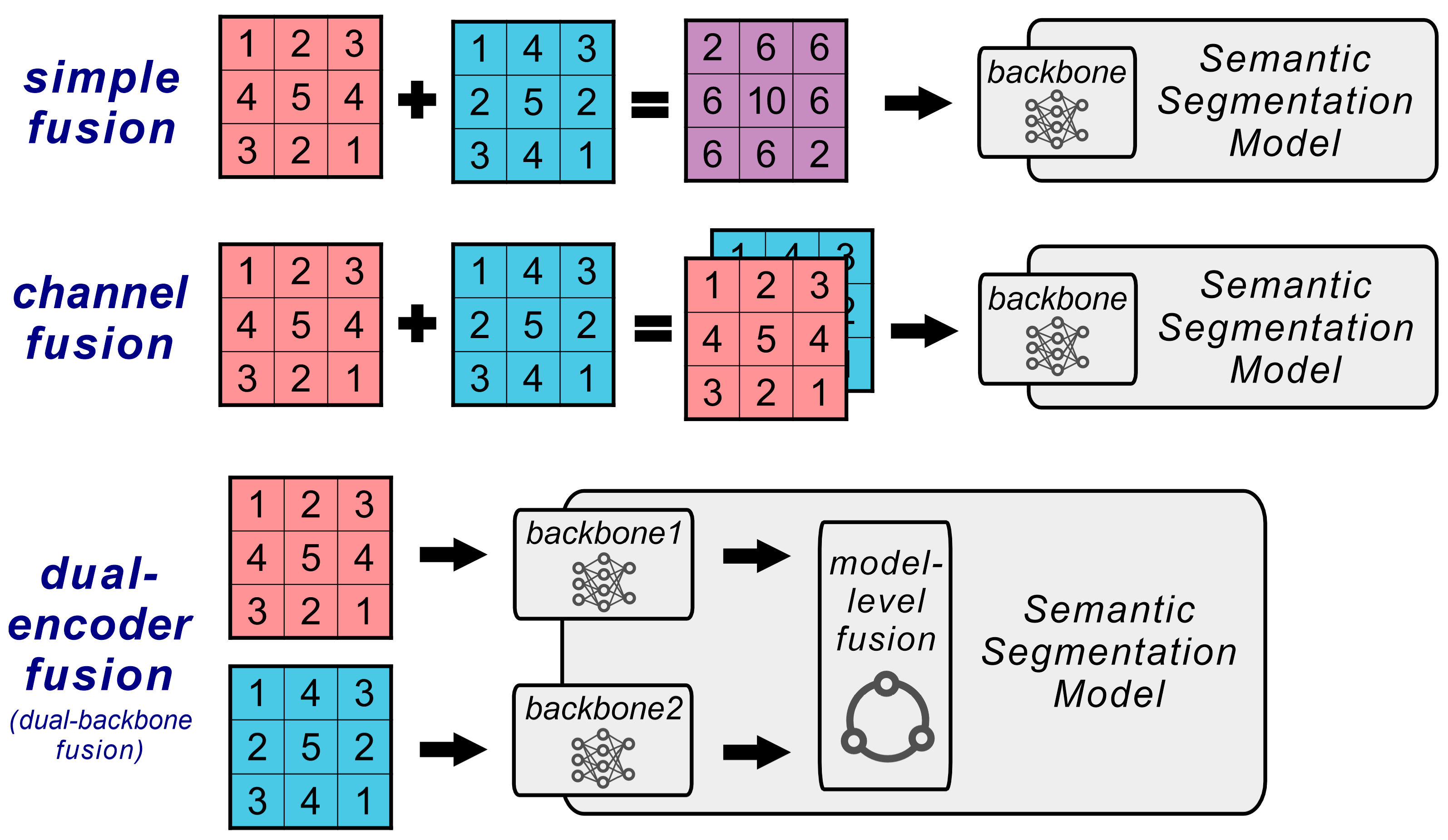
3.2.2. Encoders Design
3.2.3. Model Architecture
- (1)
- Encoder1
- (2)
- Encoder2
- (3)
- Mixer
- (4)
- Decoder
3.2.4. Improved Loss Function
3.3. Training Strategy
3.4. Evaluation Metrics
4. Results
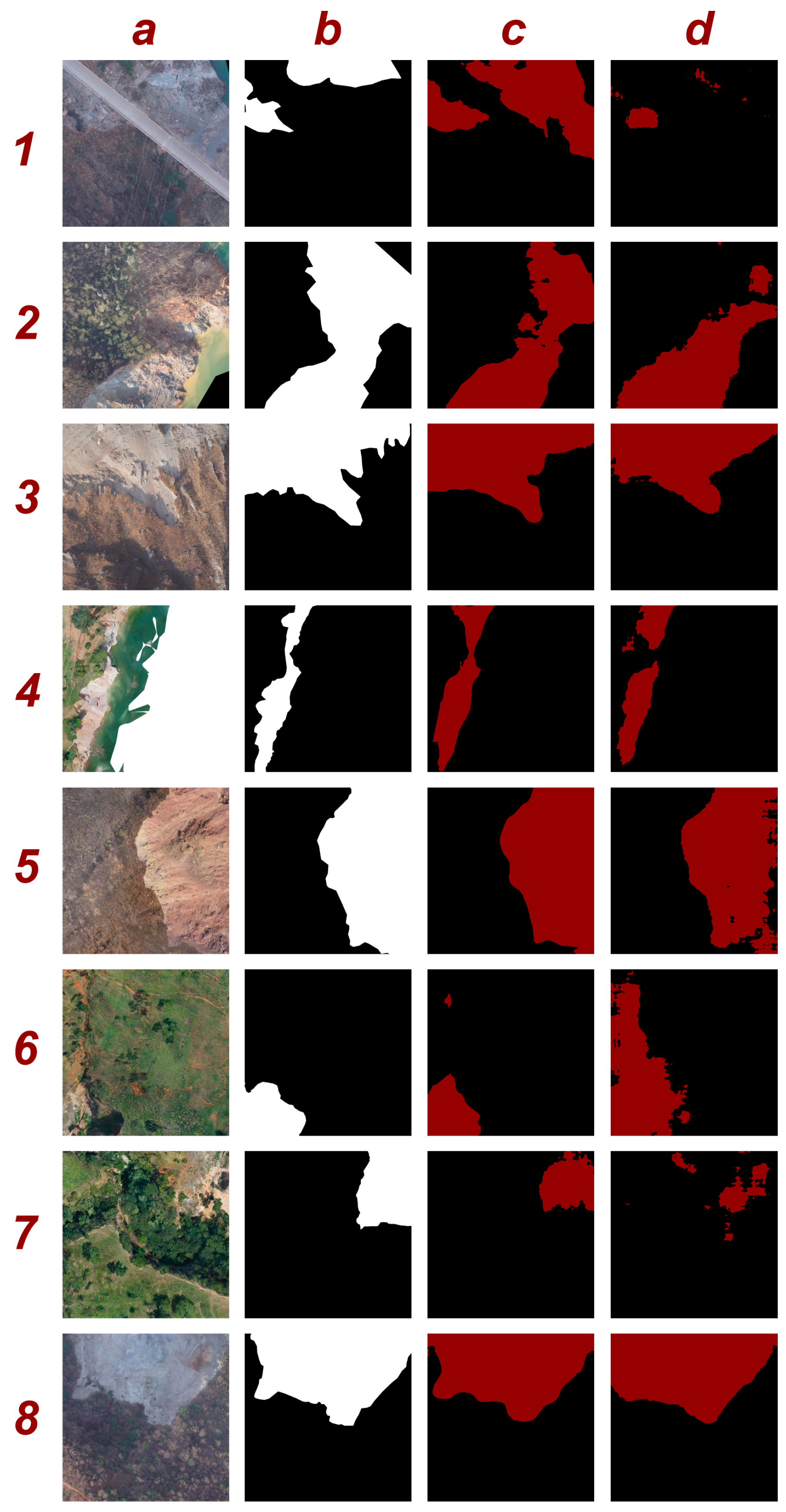
4.1. Segmentation Results and Comparison Experiments
4.2. Ablation Experiments
- (1)
- The contribution of the new combination of loss functions.
- (2)
- The contribution of the Mixer module.
- (3)
- The contribution of the dual-encoder architecture.
5. Discussion
5.1. Topographic Features in Landslide Segmentation
5.2. Mixer of DeepLab4LS Model
5.3. Loss Function in Landslide Segmentation
6. Conclusions
Author Contributions
Funding
Data Availability Statement
Acknowledgments
Conflicts of Interest
References
- Hungr, O.; Leroueil, S.; Picarelli, L. The Varnes classification of landslide types, an update. Landslides 2014, 11, 167–194. [Google Scholar] [CrossRef]
- Highland, L.M.; Bobrowsky, P. The Landslide Handbook—A Guide to Understanding Landslides; US Geological Survey: Reston, CA, USA, 2008. [Google Scholar]
- Fang, K.; Dong, A.; Tang, H.; An, P.; Wang, Q.; Jia, S.; Zhang, B. Development of an easy-assembly and low-cost multismartphone photogrammetric monitoring system for rock slope hazards. Int. J. Rock Mech. Min. 2024, 174, 105655. [Google Scholar] [CrossRef]
- Zhang, J.; Gurung, D.R.; Liu, R.; Murthy, M.S.R.; Su, F. Abe Barek landslide and landslide susceptibility assessment in Badakhshan Province, Afghanistan. Landslides 2015, 12, 597–609. [Google Scholar] [CrossRef]
- Peng, M.; Ma, C.; Shen, D.; Yang, J.; Zhu, Y. Breaching and Flood Routing Simulation of the 2018 Two Baige Landslide Dams in Jinsha River. In Dam Breach Modelling and Risk Disposal: Proceedings of the First International Conference on Embankment Dams (ICED 2020) 1; Springer: Cham, Switzerland, 2020; pp. 371–373. [Google Scholar]
- Yang, W.; Fang, J.; Jing, L.-Z. Landslide-lake outburst floods accelerate downstream slope slippage. Earth Surf. Dyn. Discuss. 2021, 9, 1251–1262. [Google Scholar] [CrossRef]
- Li, H.; Li, X.; Ning, Y.; Jiang, S.; Zhou, J. Dynamical process of the Hongshiyan landslide induced by the 2014 Ludian earthquake and stability evaluation of the back scarp of the remnant slope. Bull. Eng. Geol. Environ 2019, 78, 2081–2092. [Google Scholar] [CrossRef]
- Zhou, J.; Lu, P.; Yang, Y. Reservoir landslides and its hazard effects for the hydropower station: A case study. In Advancing Culture of Living with Landslides: Volume 2 Advances in Landslide Science; Springer: Cham, Switzerland, 2017; pp. 699–706. [Google Scholar]
- Fell, R.; Hartford, D. Landslide Risk Management. Landslide Risk Assessment; Routledge: London, UK, 2018; pp. 51–109. [Google Scholar]
- Pazzi, V.; Morelli, S.; Fanti, R. A review of the advantages and limitations of geophysical investigations in landslide studies. Int. J. Geophys. 2019, 2019, 2983087. [Google Scholar] [CrossRef]
- Giordan, D.; Adams, M.S.; Aicardi, I.; Alicandro, M.; Allasia, P.; Baldo, M.; De Berardinis, P.; Dominici, D.; Godone, D.; Hobbs, P. The use of unmanned aerial vehicles (UAVs) for engineering geology applications. Bull. Eng. Geol. Environ. 2020, 79, 3437–3481. [Google Scholar] [CrossRef]
- Rothmund, S.; Niethammer, U.; Malet, J.; Joswig, M. Landslide surface monitoring based on UAV-and ground-based images and terrestrial laser scanning: Accuracy analysis and morphological interpretation. First Break 2013, 31. [Google Scholar] [CrossRef]
- Hu, S.; Qiu, H.; Pei, Y.; Cui, Y.; Xie, W.; Wang, X.; Yang, D.; Tu, X.; Zou, Q.; Cao, P. Digital terrain analysis of a landslide on the loess tableland using high-resolution topography data. Landslides 2019, 16, 617–632. [Google Scholar] [CrossRef]
- Furukawa, F.; Laneng, L.A.; Ando, H.; Yoshimura, N.; Kaneko, M.; Morimoto, J. Comparison of RGB and multispectral unmanned aerial vehicle for monitoring vegetation coverage changes on a landslide area. Drones 2021, 5, 97. [Google Scholar] [CrossRef]
- Bui, T.; Lee, P.; Lum, K.; Loh, C.; Tan, K. Deep learning for landslide recognition in satellite architecture. IEEE Access 2020, 8, 143665–143678. [Google Scholar] [CrossRef]
- Li, Z.; Jiang, N.; Shi, A.; Zhao, L.; Xian, Z.; Luo, X.; Li, H.; Zhou, J. Reservoir landslide monitoring and mechanism analysis based on UAV photogrammetry and sub-pixel offset tracking: A case study of Wulipo landslide. Front. Earth Sci. 2024, 11, 1333815. [Google Scholar] [CrossRef]
- Hölbling, D.; Eisank, C.; Albrecht, F.; Vecchiotti, F.; Friedl, B.; Weinke, E.; Kociu, A. Comparing Manual and Semi-Automated Landslide Mapping Based on Optical Satellite Images from Different Sensors. Geosciences 2017, 7, 37. [Google Scholar] [CrossRef]
- Rosin, P.L.; Hervás, J. Remote sensing image thresholding methods for determining landslide activity. Int. J. Remote Sens. 2005, 26, 1075–1092. [Google Scholar] [CrossRef]
- Yang, X.; Chen, L. Using multi-temporal remote sensor imagery to detect earthquake-triggered landslides. Int. J. Appl. Earth Obs. Geoinf. 2010, 12, 487–495. [Google Scholar] [CrossRef]
- Eisank, C.; Smith, M.; Hillier, J. Assessment of multiresolution segmentation for delimiting drumlins in digital elevation models. Geomorphology 2014, 214, 452–464. [Google Scholar] [CrossRef]
- Rau, J.; Jhan, J.; Rau, R. Semiautomatic object-oriented landslide recognition scheme from multisensor optical imagery and DEM. IEEE Trans. Geosci. Remote Sensing 2013, 52, 1336–1349. [Google Scholar] [CrossRef]
- Liu, Q.; Wu, T.; Deng, Y.; Liu, Z. Intelligent identification of landslides in loess areas based on the improved YOLO algorithm: A case study of loess landslides in Baoji City. J. Mt. Sci. 2023, 20, 3343–3359. [Google Scholar] [CrossRef]
- Cheng, L.; Li, J.; Duan, P.; Wang, M. A small attentional YOLO model for landslide detection from satellite remote sensing images. Landslides 2021, 18, 2751–2765. [Google Scholar] [CrossRef]
- Chen, X.; Yao, X.; Zhou, Z.; Liu, Y.; Yao, C.; Ren, K. DRs-UNet: A deep semantic segmentation network for the recognition of active landslides from InSAR imagery in the three rivers region of the Qinghai–Tibet Plateau. Remote Sens. 2022, 14, 1848. [Google Scholar] [CrossRef]
- Soares, L.P.; Dias, H.C.; Grohmann, C.H. Landslide segmentation with U-Net: Evaluating different sampling methods and patch sizes. arXiv 2020, arXiv:2007.06672. [Google Scholar]
- Ding, P.; Zhang, Y.; Jia, P.; Chang, X. A comparison: Different DCNN models for intelligent object detection in remote sensing images. Neural Process. Lett. 2019, 49, 1369–1379. [Google Scholar] [CrossRef]
- Singh, R.; Rani, R. Semantic segmentation using deep convolutional neural network: A review. In Proceedings of the International Conference on Innovative Computing & Communications (ICICC), Delhi, India, 21–23 February 2020. [Google Scholar]
- Ronneberger, O.; Fischer, P.; Brox, T. U-net: Convolutional networks for biomedical image segmentation. In Proceedings of the Medical Image Computing and Computer-Assisted Intervention—MICCAI 2015: 18th International Conference, Munich, Germany, 5–9 October 2015; Proceedings, Part III 18; Springer: Cham, Switzerland, 2015; pp. 234–241. [Google Scholar]
- He, K.; Gkioxari, G.; Dollár, P.; Girshick, R. Mask r-cnn. In Proceedings of the IEEE International Conference on Computer Vision, Venice, Italy, 22–29 October 2017; pp. 2961–2969. [Google Scholar]
- Chen, L.; Zhu, Y.; Papandreou, G.; Schroff, F.; Adam, H. Encoder-decoder with atrous separable convolution for semantic image segmentation. In Proceedings of the European Conference on Computer Vision (ECCV), Munich, Germany, 8–14 September 2018; pp. 801–818. [Google Scholar]
- Yun, L.; Zhang, X.; Zheng, Y.; Wang, D.; Hua, L. Enhance the accuracy of landslide detection in UAV images using an improved Mask R-CNN Model: A case study of Sanming, China. Sensors 2023, 23, 4287. [Google Scholar] [CrossRef] [PubMed]
- Fu, Y.; Li, W.; Fan, S.; Jiang, Y.; Bai, H. CAL-Net: Conditional Attention Lightweight Network for In-Orbit Landslide Detection. IEEE Trans. Geosci. Remote Sens. 2023, 61, 4408515. [Google Scholar] [CrossRef]
- Ganerød, A.J.; Lindsay, E.; Fredin, O.; Myrvoll, T.; Nordal, S.; Rød, J.K. Globally vs. Locally Trained Machine Learning Models for Landslide Detection: A Case Study of a Glacial Landscape. Remote Sens. 2023, 15, 895. [Google Scholar] [CrossRef]
- Pepe, M.; Fregonese, L.; Crocetto, N. Use of SfM-MVS approach to nadir and oblique images generated throught aerial cameras to build 2.5 D map and 3D models in urban areas. Geocarto Int. 2022, 37, 120–141. [Google Scholar] [CrossRef]
- Dun, J.; Feng, W.; Yi, X.; Zhang, G.; Wu, M. Detection and mapping of active landslides before impoundment in the Baihetan Reservoir Area (China) based on the time-series InSAR method. Remote Sens. 2021, 13, 3213. [Google Scholar] [CrossRef]
- He, C.; Hu, X.; Tannant, D.D.; Tan, F.; Zhang, Y.; Zhang, H. Response of a landslide to reservoir impoundment in model tests. Eng. Geol. 2018, 247, 84–93. [Google Scholar] [CrossRef]
- Yi, X.; Feng, W.; Wu, M.; Ye, Z.; Fang, Y.; Wang, P.; Li, R.; Dun, J. The initial impoundment of the Baihetan reservoir region (China) exacerbated the deformation of the Wangjiashan landslide: Characteristics and mechanism. Landslides 2022, 19, 1897–1912. [Google Scholar] [CrossRef]
- Cheng, Z.; Liu, S.; Fan, X.; Shi, A.; Yin, K. Deformation behavior and triggering mechanism of the Tuandigou landslide around the reservoir area of Baihetan hydropower station. Landslides 2023, 20, 1679–1689. [Google Scholar] [CrossRef]
- Wang, D.; Gong, B.; Wang, L. On calibrating semantic segmentation models: Analyses and an algorithm. In Proceedings of the IEEE/CVF Conference on Computer Vision and Pattern Recognition, Vancouver, BC, Canada, 17–24 June 2023; pp. 23652–23662. [Google Scholar]
- Fernández, T.; Irigaray, C.; El Hamdouni, R.; Chacón, J. Methodology for landslide susceptibility mapping by means of a GIS. Application to the Contraviesa area (Granada, Spain). Nat. Hazards 2003, 30, 297–308. [Google Scholar] [CrossRef]
- Wu, C.; Hu, K.; Liu, W.; Wang, H.; Hu, X.; Zhang, X. Morpho-sedimentary and stratigraphic characteristics of the 2000 Yigong River landslide dam outburst flood deposits, eastern Tibetan Plateau. Geomorphology 2020, 367, 107293. [Google Scholar] [CrossRef]
- Chen, X.; Liu, C.; Chang, Z.; Zhou, Q. The relationship between the slope angle and the landslide size derived from limit equilibrium simulations. Geomorphology 2016, 253, 547–550. [Google Scholar] [CrossRef]
- Çellek, S. Effect of the slope angle and its classification on landslide. Nat. Hazards Earth Syst. Sci. Discuss. 2020, 2020, 1–23. [Google Scholar]
- Xiao, H.X.; Jiang, N.; Chen, X.Z.; Hao, M.H.; Zhou, J.W. Slope deformation detection using subpixel offset tracking and an unsupervised learning technique based on unmanned aerial vehicle photogrammetry data. Geol. J. 2023, 58, 2342–2352. [Google Scholar] [CrossRef]
- Taylor, L.; Nitschke, G. Improving deep learning with generic data augmentation. In Proceedings of the 2018 IEEE Symposium Series on Computational Intelligence (SSCI), Bangalore, India, 18–21 November 2018; pp. 1542–1547. [Google Scholar]
- Chlap, P.; Min, H.; Vandenberg, N.; Dowling, J.; Holloway, L.; Haworth, A. A review of medical image data augmentation techniques for deep learning applications. J. Med. Imag. Radiat. Oncol. 2021, 65, 545–563. [Google Scholar] [CrossRef] [PubMed]
- Yang, J.; Tu, J.; Zhang, X.; Yu, S.; Zheng, X. TSE DeepLab: An efficient visual transformer for medical image segmentation. Biomed. Signal Process. Control 2023, 80, 104376. [Google Scholar] [CrossRef]
- Qian, J.; Ci, J.; Tan, H.; Xu, W.; Jiao, Y.; Chen, P. Cloud detection method based on improved deeplabV3+ remote sensing image. IEEE Access 2024, 12, 9229–9242. [Google Scholar] [CrossRef]
- Baheti, B.; Innani, S.; Gajre, S.; Talbar, S. Semantic scene segmentation in unstructured environment with modified DeepLabV3+. Pattern Recognit. Lett. 2020, 138, 223–229. [Google Scholar] [CrossRef]
- He, K.; Zhang, X.; Ren, S.; Sun, J. Spatial pyramid pooling in deep convolutional networks for visual recognition. IEEE Trans. Pattern Anal. Mach. Intell. 2015, 37, 1904–1916. [Google Scholar] [CrossRef]
- Long, J.; Shelhamer, E.; Darrell, T. Fully convolutional networks for semantic segmentation. In Proceedings of the IEEE Conference on Computer Vision and Pattern Recognition, Boston, MA, USA, 7–12 June 2015; pp. 3431–3440. [Google Scholar]
- Shi, W.; Meng, F.; Wu, Q. Segmentation quality evaluation based on multi-scale convolutional neural networks. In Proceedings of the 2017 IEEE Visual Communications and Image Processing (VCIP), St. Petersburg, FL, USA, 10–13 December 2017; pp. 1–4. [Google Scholar]
- Yan, Z.; Yan, M.; Sun, H.; Fu, K.; Hong, J.; Sun, J.; Zhang, Y.; Sun, X. Cloud and cloud shadow detection using multilevel feature fused segmentation network. IEEE Geosci. Remote Sens. Lett. 2018, 15, 1600–1604. [Google Scholar] [CrossRef]
- Al-Najjar, H.A.; Kalantar, B.; Pradhan, B.; Saeidi, V.; Halin, A.A.; Ueda, N.; Mansor, S. Land cover classification from fused DSM and UAV images using convolutional neural networks. Remote Sens. 2019, 11, 1461. [Google Scholar] [CrossRef]
- Couprie, C.; Farabet, C.; Najman, L.; LeCun, Y. Indoor semantic segmentation using depth information. arXiv 2013, arXiv:1301.3572. [Google Scholar]
- Pena, J.; Tan, Y.; Boonpook, W. Semantic segmentation based remote sensing data fusion on crops detection. J. Comput. Commun. 2019, 7, 53–64. [Google Scholar] [CrossRef]
- Sun, Y.; Zuo, W.; Yun, P.; Wang, H.; Liu, M. FuseSeg: Semantic segmentation of urban scenes based on RGB and thermal data fusion. IEEE Trans. Autom. Sci. Eng. 2020, 18, 1000–1011. [Google Scholar] [CrossRef]
- Sun, Y.; Fu, Z.; Sun, C.; Hu, Y.; Zhang, S. Deep multimodal fusion network for semantic segmentation using remote sensing image and LiDAR data. IEEE Trans. Geosci. Remote Sens. 2021, 60, 5404418. [Google Scholar] [CrossRef]
- Wang, K.; He, D.; Sun, Q.; Yi, L.; Yuan, X.; Wang, Y. A novel network for semantic segmentation of landslide areas in remote sensing images with multi-branch and multi-scale fusion. Appl. Soft Comput. 2024, 158, 111542. [Google Scholar] [CrossRef]
- Sandler, M.; Howard, A.; Zhu, M.; Zhmoginov, A.; Chen, L. Mobilenetv2: Inverted residuals and linear bottlenecks. In Proceedings of the IEEE Conference on Computer Vision and Pattern Recognition, Salt Lake City, UT, USA, 18–23 June 2018; pp. 4510–4520. [Google Scholar]
- Aufar, Y.; Kaloka, T.P. Robusta coffee leaf diseases detection based on MobileNetV2 model. Int. J. Electr. Comput. Eng. 2022, 12, 6675. [Google Scholar] [CrossRef]
- Indraswari, R.; Rokhana, R.; Herulambang, W. Melanoma image classification based on MobileNetV2 network. Procedia Comput. Sci. 2022, 197, 198–207. [Google Scholar] [CrossRef]
- Ahsan, M.M.; Nazim, R.; Siddique, Z.; Huebner, P. Detection of COVID-19 patients from CT scan and chest X-ray data using modified MobileNetV2 and LIME. Healthcare 2021, 9, 1099. [Google Scholar] [CrossRef]
- He, K.; Zhang, X.; Ren, S.; Sun, J. Deep residual learning for image recognition. In Proceedings of the IEEE Conference on Computer Vision and Pattern Recognition, Las Vegas, NV, USA, 27–30 June 2016; pp. 770–778. [Google Scholar]
- Simonyan, K.; Zisserman, A. Very deep convolutional networks for large-scale image recognition. arXiv 2014, arXiv:1409.1556. [Google Scholar]
- Ma, N.; Zhang, X.; Zheng, H.; Sun, J. Shufflenet v2: Practical guidelines for efficient cnn architecture design. In Proceedings of the European Conference on Computer Vision (ECCV), Munich, Germany, 8–14 September 2018; pp. 116–131. [Google Scholar]
- Yu, H.; Chen, C.; Du, X.; Li, Y.; Rashwan, A.; Hou, L.; Jin, P.; Liu, F.F.; Kim, J.; Li, J. TensorFlow Model Garden. 2020. Available online: https://github.com/tensorflow/models (accessed on 21 December 2020).
- Zhao, H.; Shi, J.; Qi, X.; Wang, X.; Jia, J. Pyramid scene parsing network. In Proceedings of the IEEE Conference on Computer Vision and Pattern Recognition, Honolulu, HI, USA, 21–26 July 2017; pp. 2881–2890. [Google Scholar]
- Xie, E.; Wang, W.; Yu, Z.; Anandkumar, A.; Alvarez, J.M.; Luo, P. SegFormer: Simple and efficient design for semantic segmentation with transformers. Adv. Neural Inf. Process. Syst. 2021, 34, 12077–12090. [Google Scholar]
- Zhao, W.; Wang, R.; Liu, X.; Ju, N.; Xie, M. Field survey of a catastrophic high-speed long-runout landslide in Jichang Town, Shuicheng County, Guizhou, China, on July 23, 2019. Landslides 2020, 17, 1415–1427. [Google Scholar] [CrossRef]
- Jongmans, D.; Garambois, S. Geophysical investigation of landslides: A review. Bull. Société Géologique Fr. 2007, 178, 101–112. [Google Scholar] [CrossRef]
- Máttyus, G.; Luo, W.; Urtasun, R. Deeproadmapper: Extracting road topology from aerial images. In Proceedings of the IEEE International Conference on Computer Vision, Venice, Italy, 22–29 October 2017; pp. 3438–3446. [Google Scholar]
- Milletari, F.; Navab, N.; Ahmadi, S. V-net: Fully convolutional neural networks for volumetric medical image segmentation. In Proceedings of the 2016 Fourth International Conference on 3D Vision (3DV), Stanford, CA, USA, 25–28 October 2016; pp. 565–571. [Google Scholar]


| Environment and Parameters | Name and Value |
|---|---|
| Development Environment | Python 3.7.13/PyTorch 1.10.1/NVIDIA CUDA 11.3 |
| Epoch | 50 (freeze) + 450 (unfreeze) |
| Batch Size | 8 (freeze)/4 (unfreeze) |
| Optimizer | Stochastic gradient descent |
| Momentum | 0.9 |
| Weight Decay | 10−4 |
| Learning Rate | 7 × 10⁻³ (beginning)/7 × 10−5 (minimum) |
| Learning Rate Decay | Cosine annealing |
| Optical Semantic Extraction Backbone | Topographic Semantic Extraction Backbone | mIoU (%) | mPA (%) | Accuracy (%) |
|---|---|---|---|---|
| MobileNetV2 | MobileNetV2 | 76.0 | 85.3 | 92.3 |
| VGG-16 | 72.6 | 86.3 | 90.3 | |
| ShuffleNetV2 | 75.5 | 83.7 | 92.4 | |
| ResNet-18 | 74.1 | 84.1 | 91.5 | |
| ResNet-50 | 74.8 | 83.7 | 92.0 |
| Model | mIoU (%) | mPA (%) | Accuracy (%) |
|---|---|---|---|
| DeepLab4LS (with MobileNetV2 as the topographic backbone) | 76.0 | 85.3 | 92.3 |
| DeepLabV3+ | 70.5 | 80.1 | 90.4 |
| PSPNet | 70.5 | 81.2 | 90.1 |
| SegFormer | 70.1 | 77.8 | 90.8 |
| U-Net | 67.6 | 77.5 | 89.3 |
| HRNet | 69.6 | 80.0 | 89.8 |
| Base Model | Encoder1 | Encoder2 | Mixer | Loss Functions | mIoU (%) | mPA (%) | Accuracy (%) |
|---|---|---|---|---|---|---|---|
| DeepLab4LS (with MobileNetV2 as the topographic backbone) | ✔ | ✔ | ✔ | CE 2 + PE 3 | 76.0 | 85.3 | 92.3 |
| ✔ | ✔ | ✔ | CE | 72.2 | 81.2 | 91.1 | |
| ✔ | ✔ | ✔ | PE | 75.6 | 85.0 | 92.2 | |
| ✔ | ✔ | CE + PE | 74.4 | 81.7 | 92.2 | ||
| ✔ | CE + PE | 63.9 | 76.4 | 83.9 | |||
| ✔ 1 | CE + PE | 75.0 | 84.0 | 92.1 |
| Base Model | Loss Functions | mIoU (%) | mPA (%) | Precision (%) |
|---|---|---|---|---|
| DeepLab4LS (with MobileNetV2 as the topographic backbone) | CE 1 | 72.7 | 81.5 | 91.3 |
| CE + PE 2 | 76.0 | 85.3 | 92.3 | |
| CE + dice | 72.9 | 81.5 | 91.5 | |
| CE + classic SI 3 | 74.0 | 84.3 | 91.4 | |
| CE + logarithmic SI 3 | 72.2 | 82.5 | 90.8 |
Disclaimer/Publisher’s Note: The statements, opinions and data contained in all publications are solely those of the individual author(s) and contributor(s) and not of MDPI and/or the editor(s). MDPI and/or the editor(s) disclaim responsibility for any injury to people or property resulting from any ideas, methods, instructions or products referred to in the content. |
© 2024 by the authors. Licensee MDPI, Basel, Switzerland. This article is an open access article distributed under the terms and conditions of the Creative Commons Attribution (CC BY) license (https://creativecommons.org/licenses/by/4.0/).
Share and Cite
Li, Z.-H.; Shi, A.-C.; Xiao, H.-X.; Niu, Z.-H.; Jiang, N.; Li, H.-B.; Hu, Y.-X. Robust Landslide Recognition Using UAV Datasets: A Case Study in Baihetan Reservoir. Remote Sens. 2024, 16, 2558. https://doi.org/10.3390/rs16142558
Li Z-H, Shi A-C, Xiao H-X, Niu Z-H, Jiang N, Li H-B, Hu Y-X. Robust Landslide Recognition Using UAV Datasets: A Case Study in Baihetan Reservoir. Remote Sensing. 2024; 16(14):2558. https://doi.org/10.3390/rs16142558
Chicago/Turabian StyleLi, Zhi-Hai, An-Chi Shi, Huai-Xian Xiao, Zi-Hao Niu, Nan Jiang, Hai-Bo Li, and Yu-Xiang Hu. 2024. "Robust Landslide Recognition Using UAV Datasets: A Case Study in Baihetan Reservoir" Remote Sensing 16, no. 14: 2558. https://doi.org/10.3390/rs16142558
APA StyleLi, Z.-H., Shi, A.-C., Xiao, H.-X., Niu, Z.-H., Jiang, N., Li, H.-B., & Hu, Y.-X. (2024). Robust Landslide Recognition Using UAV Datasets: A Case Study in Baihetan Reservoir. Remote Sensing, 16(14), 2558. https://doi.org/10.3390/rs16142558