Abstract
As urbanization advances, the issue of urban heat islands (UHIs) grows increasingly serious, with UHIs gradually transitioning into regional urban heat islands. There is still a lack of research on the evolution and drivers of the thermal environment in urban agglomerations; therefore, in this study, we used trend analysis methods and spatial statistical analysis tools to investigate these issues in the Beijing–Tianjin–Hebei (BTH) urban agglomeration. The results demonstrated the following: (1) The land surface temperature (LST) exhibited low fluctuation, while the relative land surface temperature (RLST) fluctuated significantly. In Zhangjiakou and Chengde, the LST and RLST evolution trends were complex, and the results differed between daytime and nighttime, as well as between the annual and seasonal scales. In other regions, the trends of LST and RLST evolution were more obvious. (2) During the daytime, the high UHI clusters centered on “BJ–TJ–LF” and “SJZ–XT–HD” formed gradually; during the nighttime, the high UHI clusters were mainly observed in built-up areas. The distribution range and direction of UHIs showed greater degrees of evolution during the daytime in summer. (3) The total UHI area showed an increasing trend, and the intensity of heat stress suffered by the BTH agglomeration was increasing. (4) In BTH and Hebei, aerosol optical depth, surface solar radiation, population density, and gross domestic product were the dominant factors influencing UHIs; moreover, in Beijing and Tianjin, all factors showed an basically equal impact. The methodology and findings of this study hold significant implications for guiding urban construction, optimizing urban structure, and improving urban thermal comfort in the BTH urban agglomeration.
1. Introduction
According to the NOAA National Centers for Environmental Information (NCEI), the global average surface temperature will be 1.05 °C higher in 2023 than it was in the previous century [1], with extremely high temperatures occurring around the globe, especially in Europe [2], North America [3], and Asia [4]. Global warming has pushed approximately 9% of the world’s population, over 600 million people, beyond the boundaries of the “human climate ecological niche” [5]. Urbanization accelerates the transition from natural to man-made surfaces, and horizontal and vertical land-use patterns increase building heights, e.g., the average building height in China is 10.35 m, that in Europe is 7.37 m, and that in the United States is 6.69 m [6,7]. Changes in urban morphology affect the concentration of heat, and the imbalance in surface energy leads to higher temperatures in cities than in the surrounding areas, thus resulting in the urban heat island (UHI) phenomenon [8,9]. Currently, more than half of the world’s population lives in cities, and the UHI phenomenon affects the overall livability of cities and reduces the comfort of urban living [10]. The heat island effect also alters the ecological environment of urban areas by altering air temperature and precipitation, reducing air quality and vegetation growth [11], and even increasing the morbidity and mortality of heat-related diseases, which is a serious threat to the health of residents [12]. Therefore, exploring the evolution of urban thermal environments over a long-term time series is essential to mitigating the negative impacts of the heat island effect, improving quality of life, and ensuring sustainable urban development, especially in developing countries experiencing rapid urbanization.
With the advancement of urbanization, the distance between cities is diminishing, population movements are becoming more frequent, and intercity relationships are growing closer, leading to the gradual formation of city clusters [13]. These city clusters are spatially organized, economically connected, and highly integrated urban areas, forming the most prominent feature of urbanization in the 21st century [14]. The formation and growth of metropolitan areas have caused the scope of the UHI phenomenon to break through the boundaries of what would otherwise occur in a single city [15], and the flow of heat articulates originally isolated high-temperature regions to form regional heat islands (RHIs). The interaction between neighboring heat islands also subjects suburban and rural areas to the heat island effect [16]. Therefore, continuing to study UHIs from the perspective of single cities would underestimate the heat island intensity in urban areas and neglect its effects on rural areas, which is not conducive to urban planning and sustainable development [17]. The RHI perspective has provided new ideas for studying thermal environmental problems in urban agglomerations, such as through studies conducted in the Guangdong–Hong Kong–Macao Greater Bay Area (GBA) [18], the Yangtze River Delta (YRD) [16], and the Pearl River Delta (PRD) [19] in China, as well as in the Great Lakes Area [20] in North America and the London Metropolitan Area (LMA) in the United Kingdom [21]. The rapid population and economic growth in Beijing–Tianjin–Hebei (BTH) have made it one of the more severely heat island-affected regions in China, and some studies have shown that the region faces stronger UHI effects in the summer, with a significant seasonal pattern of diurnal heat island intensity [22].
Urban temperature is mainly characterized by air temperature (AT) and land surface temperature (LST), and the two temperatures correspond to different types of UHIs: canopy urban heat islands (CUHIs) and surface urban heat islands (SUHIs), respectively [23]. AT is mainly obtained through weather stations or in situ measurements, which offer the advantages of high temporal resolution and long-term recorded historical data. However, due to the limitations regarding the number of meteorological stations and their spatially distributed locations, CUHI studies are typically conducted at microscale levels (1–100 m) [24]. LST, on the other hand, can be obtained from remote sensing satellite images equipped with thermal infrared sensors or via algorithmic inversion; thus, the study of SUHIs can be carried out at the local scale (1–10 km), the mesoscale (10 km), or even larger spatial extents [23]. Meanwhile, SUHI research facilitates the study of how urban surface biophysical characteristics influence heat island formation and evolution [25], so SUHI data are more suitable than CUHI data for the study of regional heat island effects in urban agglomerations [17,18,26,27]. Urban heat island intensity (UHII) is an important indicator through which to study UHIs; it is generally measured by comparing the temperature difference between urban and suburban or rural areas [28]. In the process of measuring UHII, there are various methods for determining urban and suburban boundaries, such as by utilizing urban administrative boundaries, urban ring lines, the extent of urban built-up areas, or land-use types [29], and different methods for defining urban and suburban boundaries yield different results [30].
The evolution of spatial and temporal patterns in UHIs is a hot topic in the current research on heat island problems [26]. Utilizing long-term time series data enables the exploration of the intrinsic mechanism driving UHI formation and evolution and helps decision makers formulate rational urban planning and land-use policies [31], as identifying potential drivers is crucial for mitigating the heat island effect [32]. The formation and development of UHIs mainly result from the coupling of natural and socioeconomic (anthropogenic) factors [33]. Changes in urban formation also alter conditions such as light, moisture, and soil nutrients, which affect vegetation growth and thus, the urban thermal environment [34,35]; the normalized vegetation index (NDVI) is often used to study the effects of vegetation on the UHII [19]. Due to differences in surface albedo, the increase in man-made surfaces causes urban areas to absorb more solar radiation during the day, and some scholars have studied the effect of surface solar radiation (RS) on UHIs [36,37]. The heat island effect is exacerbated by the growing urban population, the continued expansion of built-up areas, and increased industrial activity. The nighttime lighting index (NTL) [27], population density (POP) [38], and gross domestic product (GDP) [39] are often used to study the impacts of socioeconomic factors on the UHI effect and air pollution due to increased energy consumption [40]. The heat island effect aggravates urban air pollution, while atmospheric aerosols trap longwave radiation, exacerbating heat island intensity, as aerosol optical depth (AOD) is related to the amount of air pollution aerosol above the observation site [40], and an increasing number of scholars have utilized AOD to quantify the impact of air pollution on the UHI effect [32,41,42].
The UHI problem is studied not only by analyzing its changes during the time series, but also by examining the evolution of the spatial distribution pattern. Some scholars have used the coefficient of variation (CV) [26], Theil–Sen trend analysis, and the Mann–Kendall trend test [17] to explore the fluctuations in the thermal environment over a long-term time series, the trends of the changes, and the significance of the trends. The evolution of UHIs in spatial distribution can be investigated using spatial statistical analyses, for which the hotspot analysis method enables the study of the spatial clustering of high or low UHII values [27]. The standard deviation ellipse (SDE) can be used to analyze changes in the direction and extent of the spatial distribution of a UHI over long periods [17,26]. Mathematical analysis models, such as ordinary least squares (OLS) [43], multiple linear regression (MLR) [42], and multiple stepwise regression (MSR) [44], have been widely used to clarify the effects of potential drivers on LST or UHIs. However, numerous studies have confirmed that the relationship between drivers and UHIs is often nonlinear; therefore, spatial analysis methods, such as the geographically weighted regression (GWR) model [45,46] and the spatial error model (SEM) [47]; and machine learning methods, such as random forests (RF), boosted regression trees (BRT), and support vector machines (SVM), have been used in heat island effect research [48,49,50]. The optimal parameters-based geographic detector (OPGD) has been widely used in UHI studies in recent years due to its immunity to the multicollinearity of variables, as well as its ability to detect relationships between drivers and geographic phenomena without linearity assumptions [18,27,51].
In this study, we aim to explore the evolution of the diurnal spatiotemporal patterns in an SUHI (hereinafter, UHI is used in place of SUHI) environment, as well as the impacts of potential drivers in the BTH urban agglomeration from 2000 to 2020. The objectives of this study are as follows: (1) to explore the volatility, trend significance, and trend persistence of LST and relative land surface temperature (RLST) changes at the pixel scale, using the CV, Sen+MK, and Sen+Hurst methods; (2) to use optimized outlier analysis and SDE to explore the spatial clustering, spatial distribution range, and evolution of the distribution direction of high or low UHII values; (3) to calculate the UHII contribution index (CI) to analyze the trend regarding the degree of heat stress over the time series; and (4) to analyze the one-way effects and two-way interactions of the drivers on the UHI using the OPGD. This study contributes to a better understanding of the spatial and temporal evolution characteristics of the UHI phenomenon, as well as its main driving factors in the BTH urban agglomeration, providing scientific suggestions for the optimization of the thermal environment in the urban agglomeration.
2. Materials and Methods
2.1. Study Area
The BTH urban agglomeration (36°05′–42°40′N,113°27′–119°50′E) is China’s “capital economic circle”, with an area of about 218,000 km2, including large, medium, and small cities, and land-use types including mainly arable land, forest land, and grassland [26]. The phenomenon of rough land use is prominent, and the expansion of construction land is disordered, which has led to a hot spot of UHI-related research issues in recent years. The urban agglomeration includes two municipalities, Beijing (BJ) and Tianjin (TJ), and 11 prefecture-level cities in Hebei Province: Baoding (BD), Tangshan (TS), Langfang (LF), Shijiazhuang (SJZ), Qinhuangdao (QHD), Zhangjiakou (ZJK), Chengde (CD), Cangzhou (CZ), Hengshui (HS), Xingtai (XT), and Handan (HD) (Figure 1).
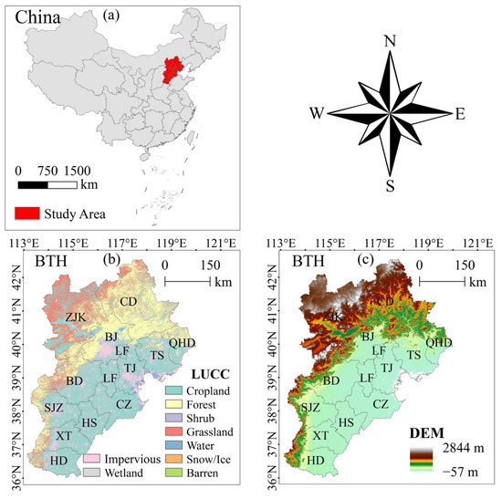
Figure 1.
(a) Location of the study area; (b) land-use/-cover type (LUCC) of the BTH urban agglomeration; (c) DEM of the BTH urban agglomeration. BJ: Beijing; TJ: Tianjin; BD: Baoding; TS: Tangshan; LF: Langfang; SJZ: Shijiazhuang; QHD: Qinhuangdao; ZJK: Zhangjiakou; CD: Chengde; CZ: Cangzhou; HS: Hengshui; XT: Xingtai; HD: Handan.
According to the Statistical Bulletin of National Economic and Social Development of the People’s Republic of China 2023, the gross regional product of BTH in 2023 was about CNY 1.04 billion, and as of 2022, the total population was about 110 million. As urbanization continues, the built-up area of the BTH urban agglomeration continues to increase. The overall topography of BTH is high in the northwest and low in the southeast, with a maximum elevation of about 2855 m. The northwest is dominated by the Taihang and Yanshan mountain ranges, and the southeast is dominated by plains. Most of the cities are located in the plains and have temperate continental monsoon climates, with hot and rainy summers and cold and dry winters, while ZJK and CD encompass mainly the northwestern mountainous areas, with relatively low temperatures [52].
2.2. Multi-Source Data
The long-term time series multi-source data used in this study include the land surface temperature [53,54], aerosol optical depth [55,56], normalized vegetation index [57], surface solar radiation [58], nighttime lighting index [59], gridded population density, and gridded gross domestic product.
LST (2000–2020) data were obtained from the National Tibetan Plateau Data Center (TPDC), https://data.tpdc.ac.cn/ (accessed on 21 February 2023), with a spatial resolution of 1 km. The Aqua MODIS LST product and GLDAS data were used as the main input data, with the vegetation index, ground surface albedo, etc., as auxiliary data. Using the high-frequency and low-frequency components of surface temperature, along with the spatial correlation of surface temperature provided in the satellite thermal infrared remote sensing and reanalysis data, a high-quality all-weather surface temperature dataset was reconstructed.
AOD (2000–2020) data were obtained from the National Earth System Science Data Center, https://www.geodata.cn/ (accessed on 1 January 2024), with a spatial resolution of 1 km. Based on multi-source big data obtained from satellite remote sensing, station observation, and model simulation, the dataset was produced using ensemble missing data reconstruction, heterogeneous data assimilation, machine learning, and multi-mode data fusion techniques to produce spatiotemporally seamless AOD datasets.
NDVI (2000–2020) data were obtained from TPDC, with a spatial resolution of 250 m. A 16-day synthetic monthly NDVI product, based on NDVI (250 m, 16 days) and land-use data from the MOD13Q1 product, were produced using preliminary reconstruction of single-period imagery with like-for-like feature noise pixels and long-term time series imagery S-G filtering techniques.
RS (2000–2017) data were derived from TPDC, with a spatial resolution of 10 km. The ISCCP-HXG product was used as the main input for the generation of surface solar radiation data for China, using geographically weighted regression and fusion of surface solar radiation site data inverted from the sunshine hours from 2261 meteorological stations in China.
NTL (2000–2020) data were obtained from Harvard Dataverse, https://dataverse.harvard.edu/ (accessed on 24 November 2023), with a spatial resolution of 500 m. The class NPP-VIIRS NTL data were constructed using a new crossover model. Sensor calibration was performed based on DMSP-OLS NTL data and NPP-VIIRS NTL data.
POP and GDP (2000–2019) data were obtained from the Resource and Environmental Science Data Center (RESDC), https://www.resdc.cn/ (accessed on 17 November 2023), with a spatial resolution of 1 km. Based on national sub-county demographic data, the data were spread onto a spatial grid using a multi-factor weight allocation method, taking into account factors such as land use, nighttime light brightness, the density of settlements, and other factors, with administrative districts as the basic statistical unit.
Due to the differences in spatial references and resolutions of the data, we processed the data to unify the spatial coordinate system and spatial resolution, finally obtaining a dataset with a spatial resolution of 1 km; then, the LST data from 2000 to 2020 were processed to obtain the seasonal (summer and winter) and annual average LST, RLST, and UHII data, as well as the six UHI driver data, including the natural factors AOD, NDVI, and RS, and the socioeconomic factors NTL, POP, and GDP. These data were processed to obtain the 2000, 2005, 2010, 2015, and 2020 seasonal and annual average data for factor detection and interaction detection analysis using the OPGD. It should be noted that, for some datasets, due to the lack of data for 2020, we used the time series from the previous year instead.
2.3. Methods
In this study, we used the CV, trend significance test (Sen+MK), and trend sustainability test (Sen+Hurst) to study the volatility of the LST and RLST changes, the significance of the change trends, and the sustainability of the change trends regarding the future of the BTH urban agglomeration from 2000 to 2020 at the pixel scale; we used spatial statistical analysis methods, such as optimized outlier Analysis, SDE, and so on, to study the spatial distribution of high- or low-value clusters of UHII and the long-term time series evolution of the spatial distribution range and distribution direction of the UHI; we calculated the UHII contribution index (CI) to study the evolution of the degree of heat stress in the BTH urban agglomeration; finally, we analyzed the factor and interaction probes of the driving factors, using the OPGD to study the influences of natural and socioeconomic factors on the UHI effect. Figure 2 shows the process framework of this study.
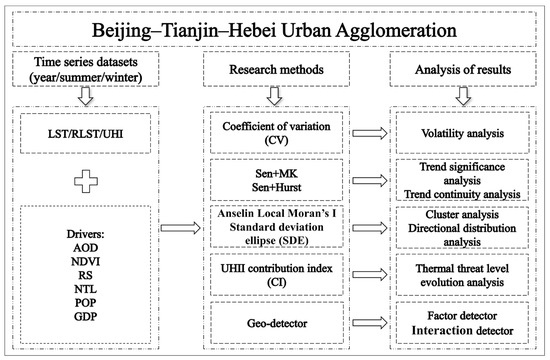
Figure 2.
Framework of the research process.
2.3.1. Relative Land Surface Temperature
The identification of the UHI extent and intensity is the key to quantitatively analyzing the heat island effect. When studying UHI evolution, RLST can effectively express the contribution of different regions to the thermal environment [17], the formula for which is as follows:
where represents one year from 2000 to 2020; represents one pixel of raster data; and denote the and of the jth pixel in the ith year, respectively; represents the number of pixel in the background temperature; represents one pixel in the background region; and denotes the of the kth pixel in the background region in the ith year. Referring to previous studies [26,60,61], the region with > 2 k is defined as the UHI region, and UHII is categorized into the following three classes: weak (L1: 2–4 k), medium (L2: 4–6 k), and strong (L3: >6 k).
2.3.2. Coefficient of Variation
The CV can be used to measure the degree of variability of the observations and is often used in geography, mainly to reflect the degree of dispersion and interannual volatility of time series data [62,63]; its formula is as follows:
where refers to the coefficient of variation of LST, denotes the standard deviation of LST, and denotes the mean value of LST. The larger the CV value, the more volatile the data; the smaller the value, the more stable the data. In this study, CV values were categorized into the following five classes: low volatility (<0.05), relatively low volatility (0.05–0.1), medium volatility (0.1–0.15), relatively high volatility (0.15–0.2), and high volatility (≥0.2) [63].
2.3.3. Theil–Sen Trend Analysis and Mann–Kendall Significance Test
The Theil–Sen trend is a robust nonparametric method [64], insensitive to outliers and effective in calculating non-normally distributed data, but it cannot test the significance of a trend [65]. The Mann–Kendall significance test determines the significance of the Theil–Sen trend; the combination of the two methods reduces the effects of outliers and is virtually immune to the interference of outlier data [63].
The Theil–Sen median is used to calculate the median slope of ( − 1)/2 data combinations, as follows:
where represents a year from 2000 to 2020, represents a pixel of the raster data, represents the trend of LST, > 0 shows an upward trend, < 0 shows a downward trend [63], and and represent the LST of the kth pixel in the jth and ith year, respectively.
The Mann–Kendall significance test of the original hypothesis implies that = 0, and there is no monotonic trend in the time series, which is calculated as follows:
The time series , = 2000, 2001, 2002, …, 2020, is constructed, and the Z statistic is defined as follows:
where and denote the LST of the kth pixel in year and year , denotes the length of the time series, is the sign function, is the variance, and the statistic is used to evaluate the significance. At a given significance level , the study series changes significantly if .
2.3.4. Hurst Analysis
The Hurst exponent was proposed by H.E. Hurst as a method for detecting the sustainability of time series data [66]; it has been widely used in geography in recent years to effectively characterize the long-term dependence of geographic data in a time series [63,64]. There are several methods of calculating the Hurst exponent, the most widely used of which is the R/S analysis method. The calculation process is as follows:
- (1)
- The time series , = 1, 2, 3, …, n is constructed;
- (2)
- The mean sequence of is constructed as follows:
- (3)
- The cumulative deviation is constructed as follows:
- (4)
- The scope is calculated as follows:
- (5)
- The standard deviation is calculated as follows:
- (6)
- The Hurst exponent is calculated as follows:
2.3.5. Anselin Local Moran’s I
According to the first law of geography, the closer the spatial distance between objects, the greater the attribute correlation and the greater the spatial dependence [69]. The Anselin Local Moran’s I tool was utilized to calculate Local Moran’s I values, z-scores, p-values, and statistically significant UHII clustering types in order to identify the spatial clustering of high- and low-value elements, as well as the distribution of outliers; the process of calculation was as follows:
where denotes the mean value of UHII; and denote the UHII at spatial locations and , respectively; is the spatial weight matrix; and is the total number of elements. In our study, we used the optimized outlier analysis tool that performs Anselin Local Moran’s I using parameters derived from input data features.
2.3.6. Directional Distribution Analysis
SDE analysis is a methodology that can effectively demonstrate the overall characteristics of the spatial distribution of geographic elements. SDEs are created to summarize the spatial characteristics of the UHII as central, discrete, and directional tendencies [70]; the formula is as follows:
where is the standard deviation of the x-axis, is the standard deviation of the y-axis, and are the coordinates of element , and and denote the mean centers of the x and y elements, respectively.
2.3.7. UHII Contribution Index
To quantify the evolution of the level of thermal threat in the BTH urban agglomeration, the contribution index of each class of UHII from 2000 to 2020 can be calculated as follows:
where refers to the area of the UHII class , and refers to the total area of the UHI.
2.3.8. Optimal Parameters-Based Geographic Detector
The OPGD is a method for detecting spatial variations in geographic phenomena and revealing their drivers [71]; this does not require the assumption of linearity; therefore, its computational process and results are not affected by variable multicollinearity [72]. The OPGD consists of four modules, namely, factor detection, interaction detection, ecological detection, and risk detection [71], and we used factor detection and interaction detection to quantify the effects of drivers on spatial heterogeneity in the UHI.
Factor detection quantifies the influence of a driver with the value, which ranges from (0, 1); the larger the value, the greater the influence. In extreme cases, a of 1 means that factor X completely controls the spatial distribution of Y, and a of 0 means that factor X is irrelevant to Y. The formula for calculating is as follows:
where the entire study area consists of cells and is divided into classes, which consist of cells, and and denote the variance of Y-values in class h and the whole region, respectively [73,74,75]. and are denoted as the Within Sum of Squares and Total Sum of Squares of the entire region, respectively.
Interaction probes were used to identify the influences of factors X on Y, i.e., whether factors X1 and X2 interact to increase or decrease the explanatory power of Y, or whether the effects of factor X on Y are independent. Factor interactions of the drivers [18,27,71] are shown in Table 1.

Table 1.
Factor interactions of drivers.
3. Results
3.1. Volatility Analysis of LST and RLST Changes
The spatial distributions of the CVs of diurnal LST and RLST at annual and seasonal scales (summer and winter) in the BTH urban agglomeration from 2000 to 2020 were significantly different (Figure 3 and Figure 4). The results showed that the spatial distributions of the CVs of LST at the interannual, summer, and winter scales during daytime and nighttime were highly similar, and LST changes showed essentially low volatility (CV < 0.05) in more than 99% of the regions in BTH. (Figure S1). The remaining regions with high fluctuations in LST changes (CV > 0.05) were distributed in the coastal region of TJ, which may be due to the sea–land interaction that makes LST changes more complex.

Figure 3.
Spatial distributions of CVs for LST in the BTH urban agglomeration from 2000 to 2020: (a) interannual daytime; (b) summer daytime; (c) winter daytime; (d) interannual nighttime; (e) summer nighttime; and (f) winter nighttime.

Figure 4.
Spatial distributions of CVs for RLST in the BTH urban agglomeration from 2000 to 2020: (a) interannual daytime; (b) summer daytime; (c) winter daytime; (d) interannual nighttime; (e) summer nighttime; and (f) winter nighttime.
Fluctuations in RLST changes were evenly distributed in most regions, except for ZJK and CD, where there were essentially none, possibly due to the higher altitudes of these two cities and the distribution of more forests, grasslands, and croplands (Figure 1), which have good cooling effects and help the RLST remain stable. Overall, the BTH urban agglomeration exhibited large fluctuations in RLST from 2000 to 2020. During the daytime, RLST fluctuations exhibited both relatively high and high volatility over about 90% of the region. At night, there were more areas exhibiting relatively low and medium fluctuations in RLST interannually, covering 61.1% of the area, and, in summer and winter, relatively high and high fluctuations were noted over 60–80% of the area (Figure S2).
3.2. LST and RLST Trend Significance Tests
The spatial distributions of trend significance tests (Sen+MK) for diurnal LST and RLST in the BTH urban agglomeration for the years from 2000 to 2020 are significantly different (Figure 5 and Figure 6). During the daytime, LST in the cities of ZJK and CD mainly decreased non-significantly for about 20% of BTH. In our opinion, this may be due to the higher elevations of the two cities, encompassing more forests, grasslands, and croplands (Figure 1). In the other regions, LST is predominantly on an upward trend, but non-significant increases cover 25–45% of the area. In the interannual and summer months, LST is mainly significantly and very significantly increasing, over a total of about 46% of the area; however, in the winter months, LST is significantly and very significantly rising, in a total of 22.1% of the area, which is a significant decrease compared to the results for the interannual and summer months, since there are more areas exhibiting non-significant increases in the winter months. At night, the LST of BTH is basically in an upward trend, but it is noteworthy that the highly significant rise covers about 65–80% of the region during the interannual and summer months, but in the winter season, the non-significant rise is observed in about 58.1% of the region, mainly in ZJK, CD, CZ, and XT (Figure 5 and Figure S3).
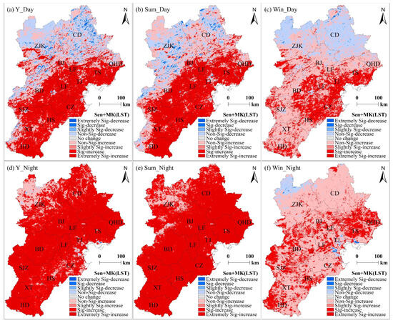
Figure 5.
Spatial distributions of LST trend significance tests (Sen+MK) for BTH urban agglomerations, 2000–2020: (a) interannual daytime; (b) summer daytime; (c) winter daytime; (d) interannual nighttime; (e) summer nighttime; and (f) winter nighttime.
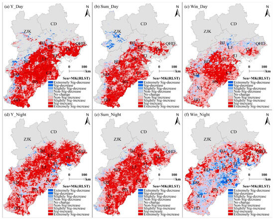
Figure 6.
Spatial distributions of RLST trend significance tests (Sen+MK) for BTH urban agglomeration, 2000–2020: (a) interannual daytime; (b) summer daytime; (c) winter daytime; (d) interannual nighttime; (e) summer nighttime; and (f) winter nighttime.
The results of the trend significance tests for RLST were essentially unchanged in ZJK and CD. During the day, the area exhibiting significant and highly significant increases in RLST reached between 16–32% in areas outside of ZJK and CD. Interannually, the area with a highly significant rise in RLST was larger, but in winter, the area showing a non-significant increase was larger. At night, the area exhibiting the non-significant increase in RLST was larger, at around 20%. In addition to this, the areas of significant and highly significant increase in RLST covered 19.2% and 27.1% of the region interannually and in summer, respectively, but in winter, the area of non-significant decrease (mainly in CZ, LF, XT, and TJ) covered only 18.5% of the region (Figure 6 and Figure S4).
3.3. LST and RLST Trend Persistence Analysis
The spatial distributions of the persistence (Sen+Hurst) of the diurnal LST and RLST trends in the BTH urban agglomeration from 2000 to 2020 are significantly different (Figure 7 and Figure 8). The results indicate that, in the future, there will be no area of random variation in LST and RLST in the BTH region. During the daytime, about 6.9% of the interannual LST trends in ZJK and CD will show a continuous decrease; however, about 20% of the LST trends in the whole BTH (mainly in ZJK and CD) will experience a change from decreasing to increasing. In the other regions in BTH, the future interannual LST trends indicate mainly a sustained increase, changing from increasing to decreasing in about 30.5% and 44.6% of the regions, respectively, while the future summer and winter LST trends mainly change from increasing to decreasing in about 64.6% and 62.5% of the regions, respectively. At nighttime, interannually, and in summer, the future LST change trends in the BTH region are continuously upward and downward, with both covering about 99% of the area, while in the winter, the future LST trend will be upward to downward over 90.5% of the area (Figure 7 and Figure S5).

Figure 7.
Spatial distributions of LST trend sustainability (Sen+Hurst) analysis for the BTH urban agglomeration in 2020–2020: (a) interannual daytime; (b) summer daytime; (c) winter daytime; (d) interannual nighttime; (e) summer nighttime; and (f) winter nighttime.
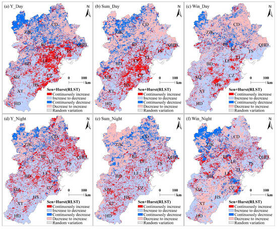
Figure 8.
Spatial distributions of RLST trend sustainability (Sen+Hurst) analysis for the BTH urban agglomeration in 2020–2020: (a) interannual daytime; (b) summer daytime; (c) winter daytime; (d) interannual nighttime; (e) summer nighttime; and (f) winter nighttime.
The RLST future change trend is more complex compared to that of the LST, comprising the following four trends: sustained increase, change from increase to decrease, sustained decrease, and a change from decrease to increase. During the daytime, the RLST future sustained decrease and a change from decrease to increase are mainly distributed in ZJK, CD, and a small portion of the surrounding area, with the proportion of sustained decrease in 10–17% and the change from decrease to increase in 27–36 of the area. In other regions, the future trends of RLST are mainly sustained increase and a change from increase to decrease, with sustained increase occupying 9–18% of the region (mainly distributed in LF, HS, BJ, and TJ) and a change from increase to decrease covering 36–46% of the region. At night, the spatial distributions of future trends in interannual and summer RLST are relatively similar, with continued decrease and change from decrease to increase mainly distributed in ZJK and CD, with both trends covering 30–40% of the region. In other regions, the interannual and summer RLST future trends are dominated by sustained increase and a change from increase to decrease; however, the change from increase to decrease will cover 45–52% of the region. During winter nights, the distribution of RLST future trends in BTH is relatively discrete, but specifically, rising-to-falling and falling-to-falling exhibit two trends covering about 77% of the region (Figure 8 and Figure S6).
3.4. UHII Anselin Local Moran’s I
ZJK and CD were largely unaffected by urban heat islands from 2000 to 2020; a few urban areas in ZJK were affected by the heat island effect during the summer daytime hours in earlier years, but this effect has been diminishing over time. Figure 9, Figure 10 and Figure 11 show the results of the analysis of diurnal UHII clustering and anomalies interannually, in summer, and in winter, respectively. Significant differences were found in the spatial distributions of the clusters of high or low daytime and nighttime UHII values, as well as in the sizes of the distribution areas. From an annual perspective, during the daytime, the regions with high UHII value clustering showed an increasing trend, from 28.7% to 37.5%. Among them, there was a significant increase from 2000 to 2005, mainly distributed in HS, CZ, and LF. The regions of UHII low-value clustering showed a decreasing trend, from 43% to 34.1%, mainly distributed in BJ, TJ, LF, BD, and TS. It can be observed that the regions with decreasing low-value clustering are mainly replaced with high-value clustering (Figure 9). At night, the UHII high-value clusters are mainly distributed in HD, XT, SJZ, BD, BJ, and TJ (mainly built-up areas), while the coverage area remains stable at around 28%. The UHII low-value clusters are mainly distributed in HS, CZ, HS, and TS (mainly outside of built-up areas), and the coverage area also remains stable, at around 44% (Figure S7).

Figure 9.
Spatial distributions of UHII Anselin Local Moran’s results for the BTH urban agglomeration from 2000 to 2020: (a) 2000 daytime; (b) 2005 daytime; (c) 2010 daytime; (d) 2015 daytime; (e) 2020 daytime; (f) 2000 nighttime; (g) 2005 nighttime; (h) 2010 nighttime; (i) 2015 nighttime; and (j) 2020 nighttime.
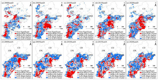
Figure 10.
Spatial distributions of UHII Anselin Local Moran’s results for the BTH urban agglomeration in summer from 2000 to 2020: (a) 2000 daytime; (b) 2005 daytime; (c) 2010 daytime; (d) 2015 daytime; (e) 2020 daytime; (f) 2000 nighttime; (g) 2005 nighttime; (h) 2010 nighttime; (i) 2015 nighttime; and (j) 2020 nighttime.

Figure 11.
Spatial distributions of UHII Anselin Local Moran’s I results for the BTH urban agglomeration in winter from 2000 to 2020: (a) 2000 daytime; (b) 2005 daytime; (c) 2010 daytime; (d) 2015 daytime; (e) 2020 daytime; (f) 2000 nighttime; (g) 2005 nighttime; (h) 2010 nighttime; (i) 2015 nighttime; and (j) 2020 nighttime.
During the summer, the area of BTH impacted by the UHI effect during the daytime is increasing (mainly in XT, HS, CZ, and TJ). The UHII high-value clusters are mainly observed in HD, XT, SJZ, LF, TS, BJ, and TJ, with an increase in the area of coverage from 24.6% to 31.4%, with increases observed in the areas of HS, LF, and, most notably, CZ. The UHII low-value clustering is mainly observed in QHD, BD, LF, XT, and HS, with a decrease in coverage area of about 6.2% to about 37.4% in 2020. At night, the UHII high-value clusters are mainly noted in HD, XT, SJZ, HS, CZ, LF, BJ, and TJ (mainly built-up areas), with a slight rise in the coverage area to 24.6% in 2020, an increase of about 4.6%. The UHII low-value clusters are mainly in SJZ, BD, LF, TS, and QHD (mainly outside of built-up areas), and, similar to the results for the daytime hours, there is a slight downward trend, at 38% in 2020, down about 3.5% (Figure 10 and Figure S8).
During the winter, the daytime UHII high-value clusters are mainly located in HD, XT, SJZ, CZ, and HS, with the coverage area growing from 32.7% to 36.9%. It is noteworthy that these cities are located in the southern part of the BTH region. However, in 2005, QHD, TS, and LF, which are located in the north, also showed UHII high-value clustering in some areas, which were gradually replaced by UHII low-value clustering over time. In 2000 and 2005, UHII low-value clusters were distributed in HS, SJZ, BD, CZ, and other regions, which were largely replaced by high-value clusters by 2010. In 2020, UHII low-value clustering was mainly distributed in BJ, TJ, QHD, LF, TS, and XT, covering about 37.1% of the area, with a decrease of about 6.1%. Unlike the daytime results, the nighttime UHII high-value clusters were mainly distributed in HD, XT, SJZ, BD, BJ, and TJ, and the coverage area is stable, at about 29%. the UHII low-value clusters were mainly distributed in HS, SJZ, LF, TS, and QHD, and the coverage area is also basically unchanged, at about 46%. The areas of UHII high- and low-value clusters are stable, but it is noteworthy that the distributions in LF and QHD are not stable at all; however, the distributions in LF, TS, and CZ are stable, in that there is no heat island effect in areas with large distributions (Figure 11 and Figure S9).
3.5. UHII Direction Distribution Analysis
Figure 12 and Table S1 show the evolution of the spatial extent and direction of distribution of UHI in the BTH region from 2000 to 2020. The results of the SDE analyses of the UHI are highly similar under all conditions, except during the daytime in the summer, both in terms of the extent of the spatial distribution and the direction of the distribution. The location of the center of the UHI is distributed at the boundaries of BD, HS, and CZ, and the center of the UHI shifts slightly along the direction of the elliptical distribution (southwest–northeast) during the time series period; the direction of the distribution remains unchanged, while the orientation angle of the five different scenario ellipses was increased by about 4°. It can be observed that the trends of both the evolution of the spatial distribution range and the direction of the distribution of the UHI remain stable.
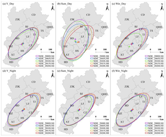
Figure 12.
2000–2020 UHII SDE analyses for the BTH urban agglomeration: (a) interannual daytime; (b) summer daytime; (c) winter daytime; (d) interannual nighttime; (e) summer nighttime; and (f) winter nighttime.
However, during the daytime in summer, there is a significant change in both the extent and direction of the spatial distribution of the UHI. Compared with other scenarios, the spatial distribution range of the UHI is larger, but there is a trend of narrowing in the distribution range. From 2000 to 2010, the center of the UHI was located in the southeast of BD, but was observed gradually moving southward; from 2010 to 2020, it gradually moved westward to CZ, and the distribution direction of the ellipse shifted along the clockwise direction. By 2020, the distribution direction had become similar to that in the other scenarios (southwest–northeast), while the ellipse direction angle is 38.41°, which is an increase of 17.18° compared to the results for 2000; these results have been verified in other studies [26]. The shift in the direction of the UHI distribution indicates that the intensity of the heat island in BJ, TJ, and LF increased from 2010 to 2020, which may be related to the rapid urbanization processes occurring in these areas in recent years.
3.6. UHII Contribution Index Analysis
Figure 13, Figure 14 and Figure 15 show the trends of UHII classes and the evolution of the total UHI area in the BTH, BJ, TJ, and HB regions from 2000 to 2020. Overall, the evolution of the UHII class in the BTH region is characterized by a gradual shrinkage of the L1 (weak, 2–4 k) region and gradual expansions of the L2 (medium, 4–6 k) and L3 (strong, >6 k) regions, with the L2 region expanding at a faster rate. On an interannual scale, the regions of UHII enhancement were larger during the day than at night. During the daytime, the area covered by BTH region L1 decreased by 53.4%, while the areas occupied by L2 and L3 increased by 35.4% and 18%, respectively. At night, the area covered by BTH area L1 decreased by 17.8%, while the areas occupied by L2 and L3 increased by 14% and 3.8%, respectively. However, it is worth noting that at night, TJ exhibits a larger proportion of L3 regions compared to the other municipalities, suggesting that TJ has a higher degree of thermal conduction at night, and the thermal comfort experience of the residents would be reduced (Figure 13).
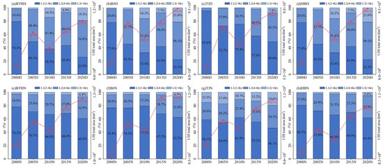
Figure 13.
Changes in the percentage of each class of UHII and the total area of the UHI from 2000 to 2020: (a) BTH daytime; (b) BJ daytime; (c) TJ daytime; (d) HB daytime; (e) BTH nighttime; (f) BJ nighttime; (g) TJ nighttime; and (h) HB nighttime. Percentage stacked plots indicate the share of each class of UHII, and curve plots indicate the change in total area of the UHI.
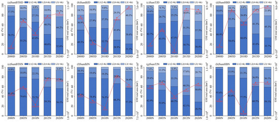
Figure 14.
Changes in the percentage of each class of UHII and the total area of the UHI in summer from 2000 to 2020: (a) BTH daytime; (b) BJ daytime; (c) TJ daytime; (d) HB daytime; (e) BTH nighttime; (f) BJ nighttime; (g) TJ nighttime; and (h) HB nighttime. Percentage stacked plots indicate the share of each class of UHII, and curve plots indicate the change in total area of the UHI.
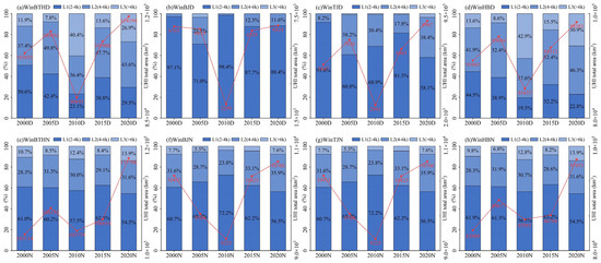
Figure 15.
Changes in the percentage of each class of UHII and the total area of the UHI in winter from 2000 to 2020: (a) BTH daytime; (b) BJ daytime; (c) TJ daytime; (d) HB daytime; (e) BTH nighttime; (f) BJ nighttime; (g) TJ nighttime; and (h) HB nighttime. Percentage stacked plots indicate the share of each class of UHII, and curve plots indicate the change in total area of the UHI.
During the summer months, the BTH regions with increased UHII were similarly greater during the day than at night, and the degree of heat stress would be higher. During the day, the L1 region decreased by 45.9%, and the L2 and L3 regions increased by 26.7% and 19.2%, respectively. In contrast, at night, the L1 region decreased by 35.7%, and the L2 and L3 regions increased by 30.6% and 5.2%, respectively. Notably, by 2020, the L3 region reached 40.3% and 32.3% in BJ and TJ, respectively, as well as 21% in the HB region, which indicates that the region of high-intensity heat stress expanded during the daytime in the summer, especially from 2010 to 2020 (Figure 14).
During the winter months, changes in UHII within the BTH region varied considerably between daytime and nighttime. During the daytime, the L1 coverage area was shrinking, while the L2 and L3 coverage areas were expanding; however, during nighttime, the proportion of UHII in each class remained essentially unchanged. Specifically, during the day, the L1 area contracted by 21.1%, and the L2 and L3 areas expanded by 6.2% and 15%, respectively, which are relatively small changes compared to those observed in the interannual and summer periods. However, it is worth noting that, within BJ and TJ, the L1 region is very highly weighted. In the territory of HB, the L1 region is smaller, but the L3 region has a higher share, reaching 30.9% in 2020. However, at night, changes in the L1, L2, and L3 regions are all relatively stable. It should be noted that the share of the L3 region in TJ is relatively high compared to in other cities, which suggests that we should pay attention to the degree of thermal stress in TJ at night during the winter (Figure 15).
The trends regarding total diurnal UHI area in BTH were similar interannually, in summer, and in winter, showing overall increasing trends, but decreasing trends from 2005 to 2010, and then increases in total area from 2010 to 2015—the same trend described above for BJ, TJ, and HB, specifically. It is also important to note that the total area of UHI in BJ was consistently decreasing during the summer and winter months of 2000–2010. In BTH, although there is a higher proportion of high-grade areas in UHII during the daytime than at night, the total area of UHI at night is larger than during the daytime, and the same result is also true, specifically for BJ, TJ, and HB, indicating that the BTH region is less impacted by the heat island effect during the day than at night, but the degree of heat stress is higher during the day; likewise, at night, the area impacted by the heat island effect is larger than that affected during the day, but the degree of heat stress is lower at night.
3.7. Factor Detection and Interaction Detection Analysis for OPGD
3.7.1. Single-Factor Effects of Drivers on UHI
Figure 16, Figure 17 and Figure 18 show the results of factor probes for the impact of drivers on the UHI from 2000 to 2020. In BTH, the drivers are sorted according to the magnitude of the q-value, AOD > POP > GDP > RS > NTL > NDVI in the daytime, and AOD > RS > POP > GDP > NTL > NDVI during the nighttime. Based on the magnitudes of the q-values, it can be determined that AOD, RS, POP, and GDP are the dominant factors. However, in BJ, TJ, and HB, different detection results were obtained. In HB, the factor detections were largely consistent with those from BTH, which is to be expected since HB occupies most of the BTH region. In BJ, during the daytime, the influences of NDVI and NTL on the UHI were significantly enhanced, in the order of AOD > NDVI > NTL > POP > GDP > RS. However, during the nighttime, the influences of NDVI and NTL were significantly reduced in comparison to those in the daytime; instead, the role of RS was enhanced, in the order of AOD > POP > GDP > RS > NTL > NDVI. The q-values of all drivers in TJ were very close to each other, and the dominant factors were not distinguished (Figure 16). We speculate that this may be due to the particular geographic location of Tianjin, which is close to the coastline, and that the interaction between sea and land differentiates the factor detection results from those of other regions.
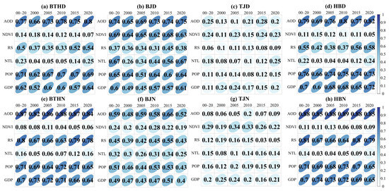
Figure 16.
Factor detection analyses of the impacts of drivers on the UHI from 2000 to 2020: (a) BTH daytime; (b) BJ daytime; (c) TJ daytime; (d) HB daytime; (e) BTH nighttime; (f) BJ nighttime; (g) TJ nighttime; and (h) HB nighttime. All results passed the significance test (ρ < 0.001).
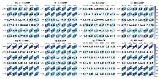
Figure 17.
Factor detection analyses of the impacts of drivers on the UHI in the summers from 2000 to 2020: (a) BTH daytime; (b) BJ daytime; (c) TJ daytime; (d) HB daytime; (e) BTH nighttime; (f) BJ nighttime; (g) TJ nighttime; and (h) HB nighttime. All results passed the significance test (ρ < 0.001).
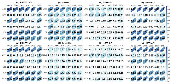
Figure 18.
Factor detection analyses of the impacts of drivers on the UHI in winter from 2000 to 2020: (a) BTH daytime; (b) BJ daytime; (c) TJ daytime; (d) HB daytime; (e) BTH nighttime; (f) BJ nighttime; (g) TJ nighttime; and (h) HB nighttime. All results passed the significance test (ρ < 0.001).
In summer, the influences of daytime drivers on the UHI in BTH varied compared to those during the interannual period, with a relatively large increase in the influence of NDVI, in the order of NDVI > AOD > POP > GDP > RS > NTL, with the dominant factors being AOD, NDVI, POP, and GDP. During the nighttime, the influences of the drivers on the UHI were essentially constant compared with those of the interannual period. Similarly, the factor detections for HB were largely consistent with those for BTH, while the detections for BJ and TJ were largely consistent with those of the interannual periods.
In winter, the factor detections of BTH, TJ, and HB were largely consistent with those of the interannual period, but there were differences in the detections for BJ, the main manifestation of which is that, during the daytime, the influence of NDVI on UHI exhibited a relatively large decrease, in the order of AOD > POP > GDP > NTL > RS > NDVI, and all the drivers can be regarded as dominant factors.
3.7.2. Double-Factor Interaction Effect of Drivers on UHI
Figure 19, Figure 20 and Figure 21 illustrate the results of the two-way interactions of the effects of drivers on the UHI, with all of the factor interactions being augmented effects (bi- or nonlinear enhancements); however, the results of the interactions can differ significantly across time and regions. Interannually, in BTH, only the interactions of NDVI with other factors were nonlinear enhancements: only NDVI ∩ RS during the daytime, and NDVI ∩ NTL, NDVI ∩ POP, and NDVI ∩ GDP during the nighttime. During the daytime, AOD had the strongest interactions with other factors; meanwhile, during the nighttime, AOD or RS had the strongest interactions with other factors. In BJ, TJ, and HB, there were significant differences in the results of interaction detection. In BJ, all interactions were bi-enhancements; in the daytime, AOD or RS interacted most strongly with other factors; at nighttime, AOD interacted most strongly with other factors. In TJ, during the day, only AOD ∩ NDVI, NDVI ∩ NTL, and NTL ∩ POP were bi-enhancements; at night, the interactions of AOD and RS with other factors showed nonlinear enhancements. In HB, only NDVI ∩ RS and NDVI ∩ NTL were nonlinear enhancements, during daytime and nighttime, respectively. During the day, AOD exhibited the strongest interactions with other factors; at night, AOD or RS showed the strongest interactions with other factors.
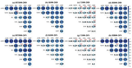
Figure 19.
Interaction detection analyses of the impacts of drivers on the UHI, from 2000 to 2020: (a) BTH daytime; (b) BJ daytime; (c) TJ daytime; (d) HB daytime; (e) BTH nighttime; (f) BJ nighttime; (g) TJ nighttime; and (h) HB nighttime. NE denotes nonlinear enhancement; no labeling denotes bi-enhancement. All results passed the significance test (ρ < 0.001).
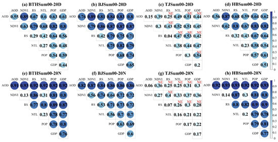
Figure 20.
Interaction detection analyses of the impacts of drivers on the UHI, in summer from 2000 to 2020: (a) BTH daytime; (b) BJ daytime; (c) TJ daytime; (d) HB daytime; (e) BTH nighttime; (f) BJ nighttime; (g) TJ nighttime; and (h) HB nighttime. NE denotes nonlinear enhancement; no labeling denotes bi-enhancement. All results passed the significance test (ρ < 0.001).
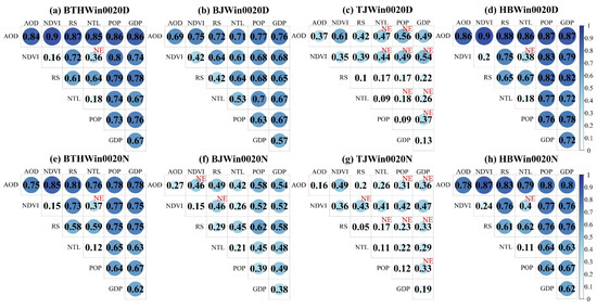
Figure 21.
Interaction detection analyses of the impacts of drivers on the UHI, in winter from 2000 to 2020: (a) BTH daytime; (b) BJ daytime; (c) TJ daytime; (d) HB daytime; (e) BTH nighttime; (f) BJ nighttime; (g) TJ nighttime; and (h) HB nighttime. NE denotes nonlinear enhancement; no labeling denotes bi-enhancement. All results passed the significance test (ρ < 0.001).
During the summer, all interaction detections resulted in bi-enhancements in BTH, BJ, and HB. In the daytime, the interactions between NDVI and other factors were the strongest; at nighttime, the interactions between AOD and other factors were the strongest. However, in TJ, during the day, AOD ∩ RS, AOD ∩ POP, AOD ∩ GDP, RS ∩ NDVI, RS ∩ NTL, RS ∩ POP, RS∩GDP, and POP ∩ GDP exhibited nonlinear enhancements; at night, AOD ∩ NDVI, AOD ∩ RS, AOD ∩ NTL, AOD ∩ POP, AOD ∩ GDP, RS ∩ NDVI, RS ∩ NTL, RS ∩ POP, and RS ∩ GDP showed nonlinear enhancements.
During the winter, in both BTH and HB, only NDVI ∩ NTL showed a nonlinear enhancement, both during daytime and at nighttime, with AOD having the strongest interactions with other factors. In BJ, the interactions of the daytime drivers were all bi-enhancements, with AOD interacting the most strongly with the other factors. At night, NDVI∩AOD and NDVI∩RS were nonlinear enhancements, while the other interactions were bi-enhancements. In TJ, during the day, NTL ∩ AOD, NTL ∩ NDVI, POP ∩ AOD, POP ∩ NDVI, POP ∩ NTL, GDP ∩ NDVI, GDP ∩ NTL, and GDP ∩ POP were nonlinear enhancements, and the interactions of AOD or NDVI with other factors were the strongest. At night, AOD ∩ POP, AOD ∩ GDP, RS ∩ NDVI, RS ∩ NTL, RS ∩ POP, RS ∩ GDP, and POP ∩ GDP were nonlinear enhancements, and NDVI showed the strongest interactions with other factors.
4. Discussion
4.1. Trend Analyses of LST and RLST Evolution
The results of the volatility analyses of LST and RLST are significantly different in that LST exhibits low volatility in all regions (CV < 0.05), while RLST does not show higher volatility (CV > 0.05) in any of the studied regions aside from in CD and ZJK (Figure 3 and Figure 4). It is obvious that the changes in LST in BTH are relatively stable, but the changes in RLST are very unstable, which also indicates that there is a significant difference between changes in LST and in background LST (suburban and rural). The prolonged effect of this difference is such that RLST shows an increasing trend in most of the BTH agglomeration (except in CD and ZJK) (Figure 6) and will continue to increase in the future if steps are not taken to control it (Figure 8). It is imperative that action should be taken to intervene; otherwise, this trend will continue to exacerbate the UHI in these areas and reduce the livability of the cities. CD and ZJK are largely unaffected by the UHI effect, which may be very much related to their altitudes and land-use/-cover types, with CD averaging 350 m above sea level, and ZJK averaging 1203 m above sea level; both areas also encompass relatively large amounts of croplands, grasslands, and forests (Figure 1). These land-cover types have better cooling effects, which can effectively reduce LST and mitigate the heat island effect, in addition to the ecological grassland construction and protection measures implemented in the two areas [76].
Using the spatial statistical tools of clustering and outlier analysis to analyze the UHII, it is determined that the UHII high-value clustering area in the BTH region continued to expand during the period from 2000 to 2020 (Figure 9, Figure 10 and Figure 11), which indicates that the scope of influence of the high-intensity heat island effect is increasing, and that more people will be affected by higher-intensity UHIs. At the same time, the spatial distributions of UHII high-value clusters during the daytime and at nighttime exhibit significant differences. Specifically, during the daytime, the UHII high-value clusters break through the original urban administrative boundaries, the distribution of the UHI effect is no longer manifested in the traditional “island” pattern of the built-up area of the city, and the high-temperature areas are gradually connected. Thus, not only will the urban area be affected by the heat island effect, but the suburbs and even the rural areas will also be impacted, forming the “high-temperature agglomeration area” centered on “BJ-TJ-LF” and “SJZ-XT-HD”, which was previously considered to be the “high-temperature agglomeration area”, as verified in previous studies [17,26]. However, at night, the clustering of high UHII values is mainly distributed in the built-up urban area, which indicates that the high-intensity heat island effect is still mainly distributed in the urban area at night, but the phenomenon of high UHII value clustering still occurs in HD and XT. This phenomenon of the heat island effect breaking through the urban boundary aggregation within urban agglomerations is known as the RHI effect, a concept pioneered by Yu et al. in 2019 [19], which pays more attention to the interactions of the heat island effect among cities within urban agglomerations, emphasizing the study of the UHI aggregation phenomenon generated by urban agglomerations as a whole [17]. Cities and rural areas are not independent, and their development is a dynamic and continuous process; thus, with the rapid development of the regional economy, the distance between cities continues to shorten, the regional energy and material flow between cities grows closer [26], the traditionally isolated UHI from the urban core area spreads to the suburbs and rural areas, and eventually, the UHIs gradually converge to form an RHI. The construction and development of urban agglomerations not only tightens economic connectivity and the flow of human circulation, but also connects the originally isolated UHI, thus changing the thermal environment in suburban and rural areas. This issue demonstrates that, when studying the regional thermal environment, we can no longer focus on the morphology and layout of a city alone, but we should start from the perspective of the urban agglomeration as a whole, as well as consider the synergistic development of cities within the urban agglomeration when formulating relevant policies.
We recorded the changes in the total area of diurnal and nocturnal UHI in the BTH, BJ, TJ, and HB regions from 2000 to 2020 and calculated the CIs of the three UHII classes in each studied year, determining that the total area of the UHI at night was larger than that during the daytime, but that the area affected by the middle (L2: 4–6 k) and high (L3: >6 k) classes of UHII during the daytime was larger than that noted during the nighttime (Figure 13, Figure 14 and Figure 15). This suggests that the area impacted by the heat island effect is more extensive at night, but the high-intensity heat island effect is more extensive during the day. Combined with Figure 9, Figure 10 and Figure 11, it can be observed that the high-intensity heat island at night is mainly concentrated in the urban built-up areas, while, in addition to the built-up areas, the suburbs and rural areas are also affected by the medium- and high-intensity UHI present during the daytime. This phenomenon may occur because during the daytime, the urban impermeable layer absorbs more solar radiation due to low albedo, while the natural surface possesses high albedo and absorbs relatively less energy, and at night, the man-made surface releases more heat, resulting in the phenomenon of high values of UHII clustering in the built-up areas of the city [45,50]. Although the total area of the UHI in the BTH region was generally on an upward trend from 2000 to 2020, the total area of the UHI decreased from 2005 to 2010, which we believe may be related to the BTH ecosystem’s joint prevention and control activities during the Beijing 2008 Olympic Games, but after the short-term joint management was over, the total area of the UHI from 2010 onwards again continued to rise, which also indicates that ecosystem management requires the adoption of a long-term regional joint prevention and control mechanism.
4.2. Impact of UHI Drivers from 2000 to 2020
The results from the factor probes of the potential drivers of the UHI effect in the BTH region show that the dominant factors are constant over the period from 2000 to 2020, as AOD, RS, POP, and GDP are significant regardless of day and night conditions. Specifically, for BJ, TJ, and HB, depending on the size of the q-value, the dominant factors change, and the factors selected in BJ and TJ can be regarded as the dominant factors, whereas the dominant factors in HB and BTH are consistent with the results for BTH, which may be because HB occupies a larger part of the BTH region (Figure 16, Figure 17 and Figure 18). The mechanisms of impact from natural and socioeconomic factors on LST are different, but both have significant effects on the UHI [27]. AOD is a key physical quantity characterizing the degree of atmospheric turbidity, and the increase in anthropogenic aerosols is closely associated with air pollution [41,42]. Both UHIs and air pollution are serious urban problems; meanwhile, they interact with each other, which seriously affects the livability of the city [32,41]. In the BTH region, AOD has always had a strong influence on the UHI effect, which suggests that we should continuously strengthen the prevention and control of air pollution, especially regarding the treatment of anthropogenic aerosol emissions. Vegetation offers good cooling effects [19], especially during the daytime, when it can absorb a large amount of solar radiation and through its own transpiration and shading effects, effectively inhibit increases in LST [77,78]. In summer, especially during the daytime, the factor detection results for NDVI also indicate that vegetation has a greater effect on UHIs.
Surfaces made of different materials have different albedos, and man-made surfaces can absorb more solar radiation compared to natural surfaces, which is a major factor contributing to the heat island effect [36,37]. Impervious layers can absorb a significant amount of solar radiation during the daytime, and then at night, when the solar radiation disappears and the surface begins to dissipate heat, man-made surfaces will release more heat than natural surfaces, which will exacerbate the heat island effect at night. Reasonable urban naturalization, orderly expansion of built-up areas, and increases in the coverage of urban vegetation can effectively mitigate the negative impacts of the UHI effect. Natural elements generally affect UHIs by directly or indirectly altering solar radiation, but socioeconomic elements are able to affect them through anthropogenic heat, while altering solar radiation [27].
NTL denotes the brightness of lights at night, which can reflect the population density, as well as the intensity of industry, especially in areas with the highest brightness levels at night, which are likely to represent industrial parks [79]; they also consume large amounts of energy and generate heat during the daytime, resulting in higher urban temperatures that are more evident in areas with higher population density and industrial development, such as BJ and TJ. Population density can indirectly reflect the degree of development in the region, as well as the complexity of the urban form [27]; the concentration of the population will intensify the expansion of the built-up area and the transformation of natural surfaces to man-made surfaces, which also implies an increase in energy consumption and anthropogenic heat emissions. Energy consumption is indispensable for economic development, and there are significant positive correlations between population size and economic output and electricity consumption [27], especially in more developed industrial areas, where socioeconomic activities consume energy, while directly (metabolic heating) or indirectly (anthropogenic heat emissions) increasing the local LST [79]. Our factor probes in the BTH region also indicate that POP and GDP are dominant factors influencing the heat island effect.
Figure 19, Figure 20 and Figure 21 show the results of factor interaction detection for the mean values of the drivers in BTH from 2000 to 2020; in the TJ region, the interactions exhibit more nonlinear enhancements, specifically the interactions between AOD and RS and other factors, which will exacerbate the impacts on the UHI. In other regions, however, the interactions between the factors are bi-enhancements, which we suggest may be because TJ is a city near the sea, and the interaction between the sea and the land complicates the intrinsic mechanism of the UHI effect [27]; this also shows that we should focus on the prevention and control of air pollution and the rational planning of the urban structure in this region. In addition, we calculated the results of interaction detection among the drivers in 2000, 2005, 2010, 2015, and 2020 (Figures S10–S15) and found that as bi-enhancements, they remained stable; however, the interactions between NDVI and other factors changed from bi-enhancements to nonlinear enhancements during the nighttime in winter between 2005 and 2010, which indicated that the impact of the interactions between NDVI and other factors on the UHI effect was intensifying, possibly related to the joint ecological and environmental management activities carried out in the BTH region during the Beijing 2008 Olympic Games, which improved the vegetation cover in the BTH area during these years.
4.3. Impact of Drivers on UHI in Built-Up Areas
Due to the continuous development of urban agglomerations, the cities within the agglomerations are more closely connected, becoming closer to each other, and the material and energy flows between the cities have led to the gradual development of the originally isolated UHI into an RHI [17,19,26]. Therefore, the results presented in Figure 19, Figure 20 and Figure 21 contain not only urban areas, but also suburban and rural areas affected by the heat island effect. To explore the impacts from urban regions, we screened out the data from urban built-up areas and conducted two-factor interaction detection analyses of the drivers separately (Figures S16–S18). It was found that, compared with the overall region, some of the interactions between NDVI and other factors would change from bi-enhancements to nonlinear enhancements in the built-up areas of BTH and HB, suggesting that the coupling of vegetation and other factors had a stronger impact on the UHI effect than individual factors in some urban built-up areas of HB, which once again demonstrates the importance of rationally planning the urban structure and enhancing the vegetation cover. The results for the built-up areas of BJ and TJ are consistent with the results of the overall region, which may be because these two municipalities have higher urbanization rates, larger built-up areas, and denser populations compared to the cities in HB, which makes their RHI phenomenon more significant. In addition, by comparing the factor interaction detection results of the urban built-up area and the whole region, combined with the results of UHII clustering and outlier analysis (Section 4.4), we found that, from 2000 to 2020, the heat island management of the BTH urban agglomeration was gradually forming an RHI centered on “BJ–TJ–LF” and “SJZ–XT–HD”. Therefore, we believe that the governance of heat islands in the BTH urban agglomeration can no longer adopt the strategy of individual governance in each city, but should formulate and implement the policy of joint governance of the BTH ecosystem from the perspective of the urban agglomeration, and coordinate this change, shifting from the governance of the UHI to the governance of the RHI.
4.4. Policy for Mitigating the UHI in BTH
The heat island effect in the BTH region is gradually evolving from UHIs to an RHI, and strategies for mitigating the UHI effect should be developed by integrating urban characteristics from the perspective of the urban agglomeration as a whole. Forests and grasslands can regulate local climate patterns, and it is important to continue to adhere to the grassland ecological construction and protection measures implemented in ZJK and CD [76], as well as to strengthen the protection of forest ecosystems, which can mitigate the heat island effect from the surrounding cities, to a certain extent. Combining the results of the UHI driver factor and interaction detection, we suggest strengthening the management of air pollution to attenuate its enhancement effect on UHII, strengthening the supervision of related sewage enterprises, and reducing anthropogenic pollutant emissions. We also recommend reasonable urban planning, less disorderly expansion of impermeable layers, and increased vegetation coverage in built-up areas. For areas with higher urbanization rates and more developed industries in BJ and TJ, it is necessary to optimize the urban, industrial, and energy structures, as the increasing concentration of the urban population will increase energy consumption and release more heat [27], and the process of the “rural revitalization” strategy should be accelerated to liberate the rural labor force and relieve the pressure on the urban population.
4.5. Limitations and Future Research
In this study, we analyzed the trends of LST and RLST in a long-term time series of BTH urban agglomeration from multiple perspectives, as well as the factor detection and interaction detection of UHI drivers, but there are still some limitations that need to be improved upon in future work. Firstly, there are multiple spatial resolutions of the data we selected, and some of them have lower accuracy (1 km and 10 km); in addition, due to some data missing for 2020, we employed the data closest to that for 2020 instead. Secondly, we analyzed the results of factor detection and interaction detection for BTH, BJ, TJ, and HB, which will allow us to study each prefecture-level city within the BTH urban agglomeration more specifically in the future. Moreover, we selected only six drivers, including natural factors (AOD, NDVI, and RS) and socioeconomic factors (NTL, POP, and GDP), and more drivers can be included in future studies for a more comprehensive understanding of the intrinsic mechanisms of the heat island effect. Finally, the factor detectors we used did not identify the impact of the directions of influence (positive or negative effect) for the drivers on the UHI effect, and the interaction detectors could only identify the results of interactions between two factors, and not interactions among three or more factors. Examining the higher-order interactions among the drivers could provide a more nuanced understanding of the intrinsic mechanisms behind UHI formation.
5. Conclusions
In this study, using the BTH urban agglomeration as the study area, the impact of the long-term time series evolution of LST and RLST on the image metric scale from 2000 to 2020 was analyzed for volatility, trend significance, and trend sustainability using CV, Sen+MK, and Sen+Hurst; Anselin Local Moran I and SDE analyses were used to study the UHII high- and low-value clusters in the spatial distribution, spatial distribution range, and distribution direction evolution; CIs were calculated to analyze the evolution of heat stress levels; and the OPGD was used to measure the one- and two-way interaction effects of the drivers on the UHI effect; the main conclusions can be summarized as follows:
- (1)
- The LST change exhibited low volatility, and the RLST change was more volatile, but there was no volatility in the RLST changes in ZJK or CD. During the daytime, LST does not decrease significantly in ZJK and CD, but increases significantly in other regions (|Z| ≥ 1.96); during the nighttime, LST increases very significantly interannually and in the summer (|Z| ≥ 2.58). RLST is essentially unchanged in ZJK and CD. During winter nights, RLST declined significantly in some regions of LF, TJ, CZ, SJZ, and XT, and increased significantly in some regions of QHD, TS, BJ, BD, HS, HD, and SJZ. In the other scenarios, it rose significantly in most regions (|Z| ≥ 1.96). Daytime LST trends changed from decreasing to increasing in most regions of ZJK and CD; meanwhile, in summer and winter, most of the other regions switched from rising to falling trends, while for still more regions, they continued to rise interannually. Nighttime LST trends continued to rise in most regions during the interannual and summer months, but BTH largely switched from a rising to a falling trend during the winter months. RLST trends switched from falling to rising in most regions of ZJK and CD; meanwhile, nighttime RLST trends went from falling to rising in parts of LF, TJ, CZ, SJZ, and XT during the winter months, and most of the region went from rising to falling trends in the other scenarios.
- (2)
- During the daytime, the UHI gradually formed a high-value clustering area centered on “BJ–TJ–LF” and “SJZ–XT–HD”, while at night, the high-value clusters of the UHI were mainly distributed in the built-up areas of the city. At the same time, the heat island effect in the BTH urban agglomeration gradually changed from that of a UHIs to an RHI, and the direction of the spatial distribution range of the UHI changed greatly during the daytime in summer.
- (3)
- The total UHI area showed an increasing trend from 2000 to 2020, but decreased from 2005 to 2010. More recently, the degree of heat stress is increasing, the share of the L1 area is gradually decreasing, and the shares of the L2 and L3 areas are increasing.
- (4)
- In BTH and HB, AOD, RS, POP, and GDP were the dominant factors impacting the UHI effect; however, in BJ and TJ, all factors affected it. In BTH, BJ, and TJ, the interaction detection results were largely bi-enhancements, while in TJ, the results were dominated by nonlinear enhancements. The effects of separate driver interactions on the UHI in the built-up areas are largely consistent with the results for the region as a whole.
In this study, by detecting and analyzing the long-term time series thermal environment evolution trend and its related drivers, we provide a deeper understanding of the intrinsic mechanisms behind UHI formation and evolution, which can provide scientific guidance for the management planning of the BTH urban agglomeration.
Supplementary Materials
The following supporting information can be downloaded at: https://www.mdpi.com/article/10.3390/rs16142601/s1, Figure S1: Percentage of LST CV by class for the BTH urban agglomeration from 2000 to 2020; Figure S2: Percentage of RLST CV by class for the BTH urban agglomeration from 2000 to 2020; Figure S3: Percentage of LST Sen+MK results for BTH urban agglomerations, 2000–2020; Figure S4: Percentage of RLST Sen+MK results for BTH urban agglomerations, 2000–2020; Figure S5: Percentage of results from the LST Sen+Hurst for the BTH urban agglomeration, 2000–2020; Figure S6: Percentage of results from the RLST Sen+Hurst for the BTH urban agglomeration, 2000–2020; Figure S7: Percentage of UHII Anselin Local Moran’s I results for the BTH urban agglomeration from 2000 to 2020; Figure S8: Percentage of UHII Anselin Local Moran’s I results for the BTH urban agglomeration in summer from 2000 to 2020; Figure S9: Percentage of UHII Anselin Local Moran’s I results for the BTH urban agglomeration in winter from 2000 to 2020; Figure S10: Interaction detection analysis of the effect of BTH urban agglomeration drivers on daytime UHI; Figure S11: Interaction detection analysis of the effect of BTH urban agglomeration drivers on nighttime UHI; Figure S12: Interaction detection analysis of the effect of BTH city cluster drivers on summer daytime UHI; Figure S13: Interaction detection analysis of the effect of BTH city cluster drivers on summer nighttime UHI; Figure S14: Interaction detection analysis of the effect of BTH city cluster drivers on winter daytime UHI; Figure S15: Interaction detection analysis of the effect of BTH city cluster drivers on winter daytime UHI; Figure S16: Interaction detection analysis of the impact of drivers on UHI in urban areas for 2000–2020; Figure S17: Interaction detection analysis of the impact of drivers on UHI in urban areas for 2000–2020; Figure S18: Interaction detection analysis of the impact of drivers on UHI in urban areas in winter for 2000–2020; Table S1: Parameters of the results of the UHI SDE analysis for the BTH urban agglomeration, 2000–2020.
Author Contributions
Conceptualization, H.L., H.Z. and L.W.; data curation, H.L. and Y.D.; formal analysis, H.L. and H.Z.; funding acquisition, L.W.; investigation, H.Z.; methodology, H.L. and H.Z.; project administration, L.W.; resources, L.W.; software, H.L. and J.Z.; supervision, L.W.; validation, H.Z. and Y.D.; visualization, H.L. and J.C.; writing—original draft, H.L. and H.Z.; writing—review and editing, H.L., Y.D., J.C. and J.Z. The first two authors contributed equally to this work and should be considered co-first authors. All authors have read and agreed to the published version of the manuscript.
Funding
This research was funded by the National Natural Science Foundation of China (grant number 42005031), the Key projects of Guangxi Natural Science Foundation (grant number 2022GXNSFDA035067), the National Natural Science Foundation of China (grant number 42272298) and the Science and Technology Development Project of Henan Province, China (grant number 222102110419).
Data Availability Statement
The datasets generated and/or analyzed during the current study are open access datasets or are available from the corresponding author on reasonable request.
Acknowledgments
We thank the reviewers who provided valuable comments to improve the paper.
Conflicts of Interest
The authors declare no conflicts of interest.
References
- Lin, Z.; Xu, H.; Yao, X.; Yang, C.; Ye, D. How Does Urban Thermal Environmental Factors Impact Diurnal Cycle of Land Surface Temperature? A Multi-Dimensional and Multi-Granularity Perspective. Sustain. Cities Soc. 2024, 101, 105190. [Google Scholar] [CrossRef]
- Sánchez-Benítez, A.; García-Herrera, R.; Barriopedro, D.; Sousa, P.M.; Trigo, R.M. June 2017: The Earliest European Summer Mega-Heatwave of Reanalysis Period. Geophys. Res. Lett. 2018, 45, 1955–1962. [Google Scholar] [CrossRef]
- Zhang, X.; Zhou, T.; Zhang, W.; Ren, L.; Jiang, J.; Hu, S.; Zuo, M.; Zhang, L.; Man, W. Increased Impact of Heat Domes on 2021-Like Heat Extremes in North America under Global Warming. Nat. Commun. 2023, 14, 1690. [Google Scholar] [CrossRef]
- He, B.-J.; Wang, J.; Zhu, J.; Qi, J. Beating the Urban Heat: Situation, Background, Impacts and the Way Forward in China. Renew. Sustain. Energy Rev. 2022, 161, 112350. [Google Scholar] [CrossRef]
- Lenton, T.M.; Xu, C.; Abrams, J.F.; Ghadiali, A.; Loriani, S.; Sakschewski, B.; Zimm, C.; Ebi, K.L.; Dunn, R.R.; Svenning, J.-C.; et al. Quantifying the Human Cost of Global Warming. Nat. Sustain. 2023, 6, 1237–1247. [Google Scholar] [CrossRef]
- Li, M.; Koks, E.; Taubenböck, H.; van Vliet, J. Continental-Scale Mapping and Analysis of 3D Building Structure. Remote Sens. Environ. 2020, 245, 111859. [Google Scholar] [CrossRef]
- Sun, F.; Liu, M.; Wang, Y.; Wang, H.; Che, Y. The Effects of 3D Architectural Patterns on the Urban Surface Temperature at a Neighborhood Scale: Relative Contributions and Marginal Effects. J. Clean. Prod. 2020, 258, 120706. [Google Scholar] [CrossRef]
- Oke, T.R. The Energetic Basis of the Urban Heat Island. Q. J. R. Meteorol. Soc. 1982, 108, 1–24. [Google Scholar] [CrossRef]
- Oke, T.R. The Urban Energy Balance. Prog. Phys. Geogr. Earth Environ. 2016, 12, 471–508. [Google Scholar] [CrossRef]
- Shen, H.; Huang, L.; Zhang, L.; Wu, P.; Zeng, C. Long-Term and Fine-Scale Satellite Monitoring of the Urban Heat Island Effect by the Fusion of Multi-Temporal and Multi-Sensor Remote Sensed Data: A 26-Year Case Study of the City of Wuhan in China. Remote Sens. Environ. 2016, 172, 109–125. [Google Scholar] [CrossRef]
- Zhang, H.; Wu, C.; Chen, W.; Huang, G. Effect of Urban Expansion on Summer Rainfall in the Pearl River Delta, South China. J. Hydrol. 2019, 568, 747–757. [Google Scholar] [CrossRef]
- Yin, Q.; Wang, J.; Ren, Z.; Li, J.; Guo, Y. Mapping the Increased Minimum Mortality Temperatures in the Context of Global Climate Change. Nat. Commun. 2019, 10, 4640. [Google Scholar] [CrossRef] [PubMed]
- Xu, X.; Pei, H.; Wang, C.; Xu, Q.; Xie, H.; Jin, Y.; Feng, Y.; Tong, X.; Xiao, C. Long-Term Analysis of the Urban Heat Island Effect Using Multisource Landsat Images Considering Inter-Class Differences in Land Surface Temperature Products. Sci. Total Environ. 2023, 858, 159777. [Google Scholar] [CrossRef] [PubMed]
- Fang, C.; Yu, D. Urban Agglomeration: An Evolving Concept of an Emerging Phenomenon. Landsc. Urban Plan. 2017, 162, 126–136. [Google Scholar] [CrossRef]
- Wang, Z.; Zhu, P.; Zhou, Y.; Li, M.; Lu, J.; Huang, Y.; Deng, S. Evidence of Relieved Urban Heat Island Intensity during Rapid Urbanization through Local Climate Zones. Urban Clim. 2023, 49, 101537. [Google Scholar] [CrossRef]
- Du, H.; Wang, D.; Wang, Y.; Zhao, X.; Qin, F.; Jiang, H.; Cai, Y. Influences of Land Cover Types, Meteorological Conditions, Anthropogenic Heat and Urban Area on Surface Urban Heat Island in the Yangtze River Delta Urban Agglomeration. Sci. Total Environ. 2016, 571, 461–470. [Google Scholar] [CrossRef] [PubMed]
- Li, Y.; Qiao, X.; Wang, Y.; Liu, L. Spatiotemporal Patterns and Influencing Factors of Remotely Sensed Regional Heat Islands from 2001 to 2020 in Zhengzhou Metropolitan Area. Ecol. Indic. 2023, 155, 111026. [Google Scholar] [CrossRef]
- Feng, R.; Wang, F.; Wang, K.; Wang, H.; Li, L. Urban Ecological Land and Natural-Anthropogenic Environment Interactively Drive Surface Urban Heat Island: An Urban Agglomeration-Level Study in China. Environ. Int. 2021, 157, 106857. [Google Scholar] [CrossRef] [PubMed]
- Yu, Z.; Yao, Y.; Yang, G.; Wang, X.; Vejre, H. Spatiotemporal Patterns and Characteristics of Remotely Sensed Region Heat Islands during the Rapid Urbanization (1995–2015) of Southern China. Sci. Total Environ. 2019, 674, 242–254. [Google Scholar] [CrossRef]
- Lowe, S.A. An Energy and Mortality Impact Assessment of the Urban Heat Island in the US. Environ. Impact Assess. Rev. 2016, 56, 139–144. [Google Scholar] [CrossRef]
- Jones, P.D.; Lister, D.H. The Urban Heat Island in Central London and Urban-Related Warming Trends in Central London since 1900. Weather 2009, 64, 323–327. [Google Scholar] [CrossRef]
- Liu, Y.; Fang, X.; Xu, Y.; Zhang, S.; Luan, Q. Assessment of Surface Urban Heat Island across China’s Three Main Urban Agglomerations. Theor. Appl. Climatol. 2017, 133, 473–488. [Google Scholar] [CrossRef]
- Peng, W.; Wang, R.; Duan, J.; Gao, W.; Fan, Z. Surface and Canopy Urban Heat Islands: Does Urban Morphology Result in the Spatiotemporal Differences? Urban Clim. 2022, 42, 101136. [Google Scholar] [CrossRef]
- Liu, H.; Huang, B.; Zhan, Q.; Gao, S.; Li, R.; Fan, Z. The Influence of Urban Form on Surface Urban Heat Island and Its Planning Implications: Evidence from 1288 Urban Clusters in China. Sustain. Cities Soc. 2021, 71, 102987. [Google Scholar] [CrossRef]
- Buyantuyev, A.; Wu, J. Urban Heat Islands and Landscape Heterogeneity: Linking Spatiotemporal Variations in Surface Temperatures to Land-Cover and Socioeconomic Patterns. Landsc. Ecol. 2009, 25, 17–33. [Google Scholar] [CrossRef]
- Xu, H.; Li, C.; Wang, H.; Zhou, R.; Liu, M.; Hu, Y. Long-Term Spatiotemporal Patterns and Evolution of Regional Heat Islands in the Beijing–Tianjin–Hebei Urban Agglomeration. Remote Sens. 2022, 14, 2478. [Google Scholar] [CrossRef]
- Liu, W.; Meng, Q.; Allam, M.; Zhang, L.; Hu, D.; Menenti, M. Driving Factors of Land Surface Temperature in Urban Agglomerations: A Case Study in the Pearl River Delta, China. Remote Sens. 2021, 13, 2858. [Google Scholar] [CrossRef]
- Heaviside, C.; Vardoulakis, S.; Cai, X.-M. Attribution of Mortality to the Urban Heat Island during Heatwaves in the West Midlands, UK. Environ. Health 2016, 15, S27. [Google Scholar] [CrossRef]
- Meng, Q.; Zhang, L.; Sun, Z.; Meng, F.; Wang, L.; Sun, Y. Characterizing Spatial and Temporal Trends of Surface Urban Heat Island Effect in an Urban Main Built-Up Area: A 12-Year Case Study in Beijing, China. Remote Sens. Environ. 2018, 204, 826–837. [Google Scholar] [CrossRef]
- Wang, K.; Wang, J.; Wang, P.; Sparrow, M.; Yang, J.; Chen, H. Influences of Urbanization on Surface Characteristics as Derived from the Moderate-Resolution Imaging Spectroradiometer: A Case study for the Beijing Metropolitan Area. J. Geophys. Res. Atmos. 2007, 112, S06. [Google Scholar] [CrossRef]
- Zhang, H.; Qi, Z.-f.; Ye, X.-y.; Cai, Y.-b.; Ma, W.-c.; Chen, M.-n. Analysis of Land Use/Land Cover Change, Population Shift, and Their Effects on Spatiotemporal Patterns of Urban Heat Islands in Metropolitan Shanghai, China. Appl. Geogr. 2013, 44, 121–133. [Google Scholar] [CrossRef]
- Geng, X.; Zhang, D.; Li, C.; Yuan, Y.; Yu, Z.; Wang, X. Impacts of Climatic Zones on Urban Heat Island: Spatiotemporal Variations, Trends, and Drivers in China from 2001–2020. Sustain. Cities Soc. 2023, 89, 104303. [Google Scholar] [CrossRef]
- Peng, J.; Jia, J.; Liu, Y.; Li, H.; Wu, J. Seasonal Contrast of the Dominant Factors for Spatial Distribution of Land Surface Temperature in Urban Areas. Remote Sens. Environ. 2018, 215, 255–267. [Google Scholar] [CrossRef]
- Yang, G.; Yu, Z.; Jørgensen, G.; Vejre, H. How Can Urban Blue-Green Space Be Planned for Climate Adaption in High-Latitude Cities? A Seasonal Perspective. Sustain. Cities Soc. 2020, 53, 101932. [Google Scholar] [CrossRef]
- Ren, Y.; Deng, L.-Y.; Zuo, S.-D.; Song, X.-D.; Liao, Y.-L.; Xu, C.-D.; Chen, Q.; Hua, L.-Z.; Li, Z.-W. Quantifying the Influences of Various Ecological Factors on Land Surface Temperature of Urban Forests. Environ. Pollut. 2016, 216, 519–529. [Google Scholar] [CrossRef] [PubMed]
- Lima, I.; Scalco, V.; Lamberts, R. Estimating the Impact of Urban Densification on High-Rise Office Building Cooling Loads in a Hot and Humid Climate. Energy Build. 2019, 182, 30–44. [Google Scholar] [CrossRef]
- Ren, J.; Shi, K.; Kong, X.; Zhou, H. On-Site Measurement and Numerical Simulation Study on Characteristic of Urban Heat Island in a Multi-Block Region in Beijing, China. Sustain. Cities Soc. 2023, 95, 104615. [Google Scholar] [CrossRef]
- Dewan, A.; Kiselev, G.; Botje, D.; Mahmud, G.I.; Bhuian, M.H.; Hassan, Q.K. Surface Urban Heat Island Intensity in Five Major Cities of Bangladesh: Patterns, Drivers and Trends. Sustain. Cities Soc. 2021, 71, 102926. [Google Scholar] [CrossRef]
- Li, Y.; Sun, Y.; Li, J.; Gao, C. Socioeconomic Drivers of Urban Heat Island Effect: Empirical Evidence from Major Chinese Cities. Sustain. Cities Soc. 2020, 63, 102425. [Google Scholar] [CrossRef]
- Eom, J.; Hyun, M.; Lee, J.; Lee, H. Increase in Household Energy Consumption Due to Ambient Air Pollution. Nat. Energy 2020, 5, 976–984. [Google Scholar] [CrossRef]
- Xiang, Y.; Ye, Y.; Peng, C.; Teng, M.; Zhou, Z. Seasonal Variations for Combined Effects of Landscape Metrics on Land Surface Temperature (LST) and Aerosol Optical Depth (AOD). Ecol. Indic. 2022, 138, 108810. [Google Scholar] [CrossRef]
- Ngarambe, J.; Joen, S.J.; Han, C.-H.; Yun, G.Y. Exploring the Relationship between Particulate Matter, CO, SO2, NO2, O3 and Urban Heat Island in Seoul, Korea. J. Hazard. Mater. 2021, 403, 123615. [Google Scholar] [CrossRef]
- Su, H.; Han, G.; Li, L.; Qin, H. The Impact of Macro-Scale Urban Form on Land Surface Temperature: An Empirical Study Based on Climate Zone, Urban Size and Industrial Structure in China. Sustain. Cities Soc. 2021, 74, 103217. [Google Scholar] [CrossRef]
- Peng, S.; Feng, Z.; Liao, H.; Huang, B.; Peng, S.; Zhou, T. Spatial-Temporal Pattern of, and Driving Forces For, Urban Heat Island in China. Ecol. Indic. 2019, 96, 127–132. [Google Scholar] [CrossRef]
- Gao, Y.; Zhao, J.; Yu, K. Effects of Block Morphology on the Surface Thermal Environment and the Corresponding Planning Strategy Using the Geographically Weighted Regression Model. Build. Environ. 2022, 216, 109037. [Google Scholar] [CrossRef]
- Wu, Z.; Tong, Z.; Wang, M.; Long, Q. Assessing the Impact of Urban Morphological Parameters on Land Surface Temperature in the Heat Aggregation Areas with Spatial Heterogeneity: A Case Study of Nanjing. Build. Environ. 2023, 235, 110232. [Google Scholar] [CrossRef]
- Bartesaghi-Koc, C.; Osmond, P.; Peters, A. Innovative Use of Spatial Regression Models to Predict the Effects of Green Infrastructure on Land Surface Temperatures. Energy Build. 2022, 254, 111564. [Google Scholar] [CrossRef]
- Shafizadeh-Moghadam, H.; Weng, Q.; Liu, H.; Valavi, R. Modeling the Spatial Variation of Urban Land Surface Temperature in Relation to Environmental and Anthropogenic Factors: A Case Study of Tehran, Iran. GIScience Remote Sens. 2020, 57, 483–496. [Google Scholar] [CrossRef]
- Masoudi, M.; Tan, P.Y. Multi-Year Comparison of the Effects of Spatial Pattern of Urban Green Spaces on Urban Land Surface Temperature. Landsc. Urban Plan. 2019, 184, 44–58. [Google Scholar] [CrossRef]
- Xu, H.; Li, C.; Hu, Y.; Li, S.; Kong, R.; Zhang, Z. Quantifying the Effects of 2D/3D Urban Landscape Patterns on Land Surface Temperature: A Perspective from Cities of Different Sizes. Build. Environ. 2023, 233, 110085. [Google Scholar] [CrossRef]
- You, M.; Huang, J.; Guan, C. Are New Towns Prone to Urban Heat Island Effect? Implications for Planning Form and Function. Sustain. Cities Soc. 2023, 99, 104939. [Google Scholar] [CrossRef]
- Feng, Z.; Liu, D.; Zhang, Y. Water Requirements and Irrigation Scheduling of Spring Maize Using GIS and CropWat Model in Beijing-Tianjin-Hebei Region. Chin. Geogr. Sci. 2007, 17, 56–63. [Google Scholar] [CrossRef]
- Zhou, J.; Zhang, X.; Zhan, W.; Gottsche, F.-M.; Liu, S.; Olesen, F.-S.; Hu, W.; Dai, F. A Thermal Sampling Depth Correction Method for Land Surface Temperature Estimation from Satellite Passive Microwave Observation over Barren Land. IEEE Trans. Geosci. Remote Sens. 2017, 55, 4743–4756. [Google Scholar] [CrossRef]
- Zhang, X.; Zhou, J.; Gottsche, F.-M.; Zhan, W.; Liu, S.; Cao, R. A Method Based on Temporal Component Decomposition for Estimating 1-km All-Weather Land Surface Temperature by Merging Satellite Thermal Infrared and Passive Microwave Observations. IEEE Trans. Geosci. Remote Sens. 2019, 57, 4670–4691. [Google Scholar] [CrossRef]
- Bai, K.; Li, K.; Sun, Y.; Wu, L.; Zhang, Y.; Chang, N.-B.; Li, Z. Global Synthesis of Two Decades of Research on Improving PM2.5 Estimation Models from Remote Sensing and Data Science Perspectives. Earth-Sci. Rev. 2023, 241, 104461. [Google Scholar] [CrossRef]
- Bai, K.; Li, K.; Ma, M.; Li, K.; Li, Z.; Guo, J.; Chang, N.-B.; Tan, Z.; Han, D. LGHAP: The Long-Term Gap-Free High-Resolution Air Pollutant Concentration Dataset, Derived via Tensor-Flow-Based Multimodal Data Fusion. Earth Syst. Sci. Data 2022, 14, 907–927. [Google Scholar] [CrossRef]
- Gao, J.; Shi, Y.; Zhang, H.; Chen, X.; Zhang, W.; Shen, W.; Xiao, T.; Zhang, Y. China Regional 250 m Fractional Vegetation cover Data Set (2000–2022); National Tibetan Plateau Data Center/Third Pole Environ. Data Cent: Beijing, China, 2022. [Google Scholar] [CrossRef]
- Feng, F.; Wang, K. Merging High-Resolution Satellite Surface Radiation Data with Meteorological Sunshine Duration Observations over China from 1983 to 2017. Remote Sens. 2021, 13, 602. [Google Scholar] [CrossRef]
- Chen, Z.; Yu, B.; Yang, C.; Zhou, Y.; Yao, S.; Qian, X.; Wang, C.; Wu, B.; Wu, J. An Extended Time Series (2000–2018) of Global NPP-VIIRS-Like Nighttime Light Data from a Cross-Sensor Calibration. Earth Syst. Sci. Data 2021, 13, 889–906. [Google Scholar] [CrossRef]
- Chen, S.; Yu, Z.; Liu, M.; Da, L.; Faiz ul Hassan, M. Trends of the Contributions of Biophysical (Climate) and Socioeconomic Elements to Regional Heat Islands. Sci. Rep. 2021, 11, 12696. [Google Scholar] [CrossRef]
- Chen, Y.; Xie, M.; Chen, B.; Wang, H.; Teng, Y. Surface Regional Heat (Cool) Island Effect and Its Diurnal Differences in Arid and Semiarid Resource-based Urban Agglomerations. Chin. Geogr. Sci. 2022, 33, 131–143. [Google Scholar] [CrossRef]
- Gooch, J.W. Coefficient of Variation; Springer: New York, NY, USA, 2010. [Google Scholar] [CrossRef]
- Jiang, W.; Yuan, L.; Wang, W.; Cao, R.; Zhang, Y.; Shen, W. Spatio-Temporal Analysis of Vegetation Variation in the Yellow River Basin. Ecol. Indic. 2015, 51, 117–126. [Google Scholar] [CrossRef]
- Zhong, X.; Li, J.; Wang, J.; Zhang, J.; Liu, L.; Ma, J. Linear and Nonlinear Characteristics of Long-Term NDVI Using Trend Analysis: A Case Study of Lancang-Mekong River Basin. Remote Sens. 2022, 14, 6271. [Google Scholar] [CrossRef]
- Nanditha, H.S.; Reshmidevi, T.V.; Simha, L.U.; Kunhikrishnan, P. Statistical Analysis of Rainfall and Groundwater Interaction in Bhadra Catchment. Environ. Dev. Sustain. 2023, 26, 16267–16287. [Google Scholar] [CrossRef]
- Hurst, H.E. Long Term Storage Capacity of Reservoirs. Trans. Am. Soc. Civ. Eng. 1951, 116, 770–799. [Google Scholar] [CrossRef]
- Li, J.; Wang, J.; Zhang, J.; Zhang, J.; Kong, H. Dynamic Changes of Vegetation Coverage in China-Myanmar Economic Corridor over the Past 20 Years. Int. J. Appl. Earth Obs. Geoinf. 2021, 102, 102378. [Google Scholar] [CrossRef]
- Geng, S.; Zhang, H.; Xie, F.; Li, L.; Yang, L. Vegetation Dynamics under Rapid Urbanization in the Guangdong–Hong Kong–Macao Greater Bay Area Urban Agglomeration during the Past Two Decades. Remote Sens. 2022, 14, 3993. [Google Scholar] [CrossRef]
- Tobler, W.R. A Computer Movie Simulating Urban Growth in the Detroit Region. Econ. Geogr. 1970, 46, 234–240. [Google Scholar] [CrossRef]
- Furfey, P.H. A Note on Lefever’s “Standard Deviational Ellipse”. Am. J. Sociol. 1927, 33, 94–98. [Google Scholar] [CrossRef]
- Wang, J.F.; Li, X.H.; Christakos, G.; Liao, Y.L.; Zhang, T.; Gu, X.; Zheng, X.Y. Geographical Detectors-Based Health Risk Assessment and its Application in the Neural Tube Defects Study of the Heshun Region, China. Int. J. Geogr. Inf. Sci. 2010, 24, 107–127. [Google Scholar] [CrossRef]
- Hu, D.; Meng, Q.; Zhang, L.; Zhang, Y. Spatial Quantitative Analysis of the Potential Driving Factors of Land Surface Temperature in Different “Centers” of Polycentric Cities: A Case Study in Tianjin, China. Sci. Total Environ. 2020, 706, 135244. [Google Scholar] [CrossRef]
- Xi, M.; Zhang, W.; Li, W.; Liu, H.; Zheng, H. Distinguishing Dominant Drivers on LST Dynamics in the Qinling-Daba Mountains in Central China from 2000 to 2020. Remote Sens. 2023, 15, 878. [Google Scholar] [CrossRef]
- Zhang, W.; Xi, M.; Liu, H.; Zheng, H. Low sensitivity of net primary productivity to climatic factors in three karst provinces in southwest China from 1981 to 2019. Ecol. Indic. 2023, 153, 110465. [Google Scholar] [CrossRef]
- Wang, J.-F.; Zhang, T.-L.; Fu, B.-J. A Measure of Spatial Stratified Heterogeneity. Ecol. Indic. 2016, 67, 250–256. [Google Scholar] [CrossRef]
- Decision on Strengthening the Ecological Construction and Protection of Grasslands in Zhangjiakou and Chengde Areas (Full Text). Hebei For. 2019, 7, 17–20.
- Guo, G.; Wu, Z.; Chen, Y. Complex Mechanisms Linking Land Surface Temperature to Greenspace Spatial Patterns: Evidence from Four Southeastern Chinese Cities. Sci. Total Environ. 2019, 674, 77–87. [Google Scholar] [CrossRef] [PubMed]
- Logan, T.M.; Zaitchik, B.; Guikema, S.; Nisbet, A. Night and Day: The Influence and Relative Importance of Urban Characteristics on Remotely Sensed Land Surface Temperature. Remote Sens. Environ. 2020, 247, 111861. [Google Scholar] [CrossRef]
- Tripathy, B.R.; Sajjad, H.; Elvidge, C.D.; Ting, Y.; Pandey, P.C.; Rani, M.; Kumar, P. Modeling of Electric Demand for Sustainable Energy and Management in India Using Spatio-Temporal DMSP-OLS Night-Time Data. Environ. Manag. 2017, 61, 615–623. [Google Scholar] [CrossRef]

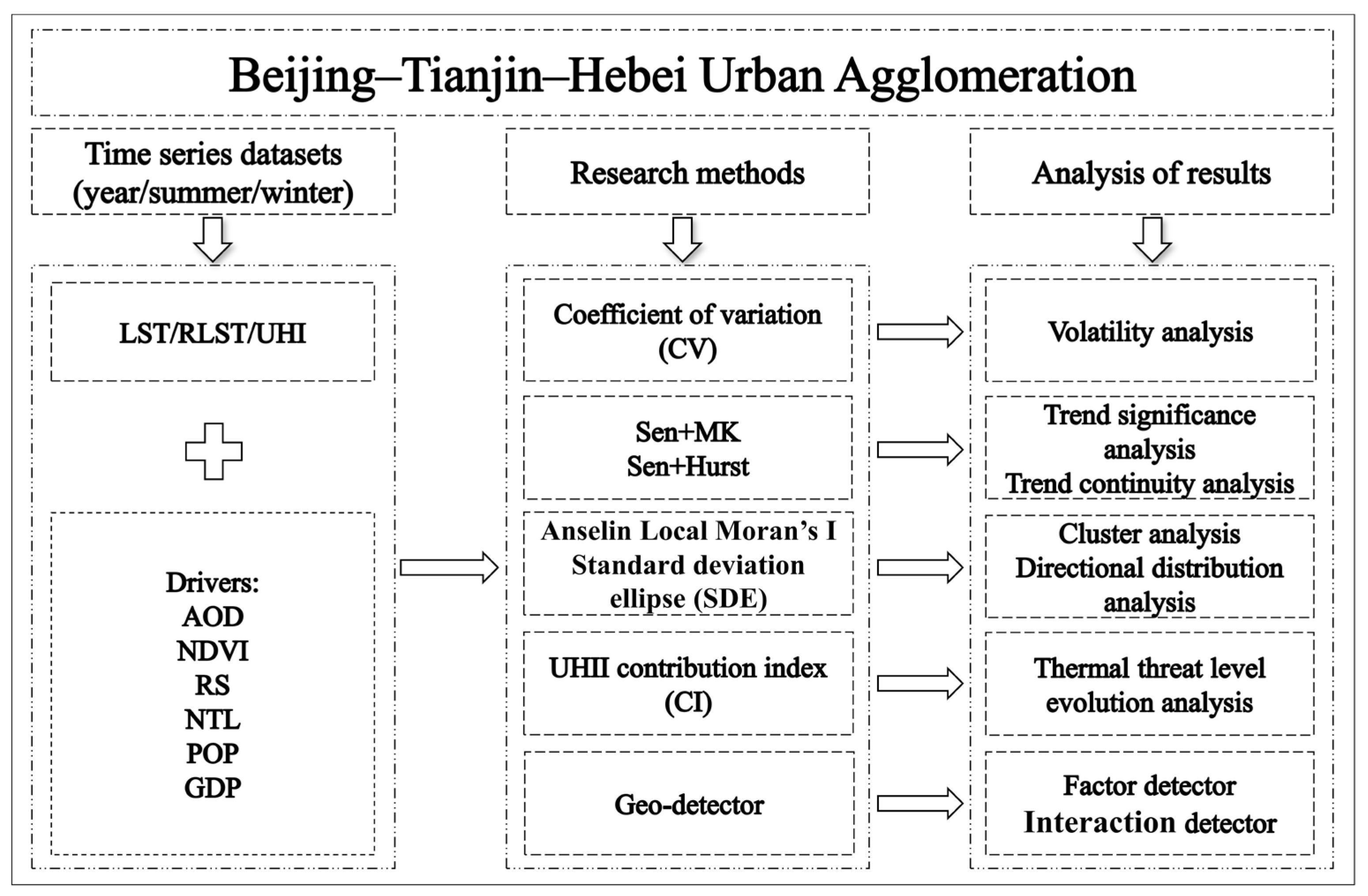
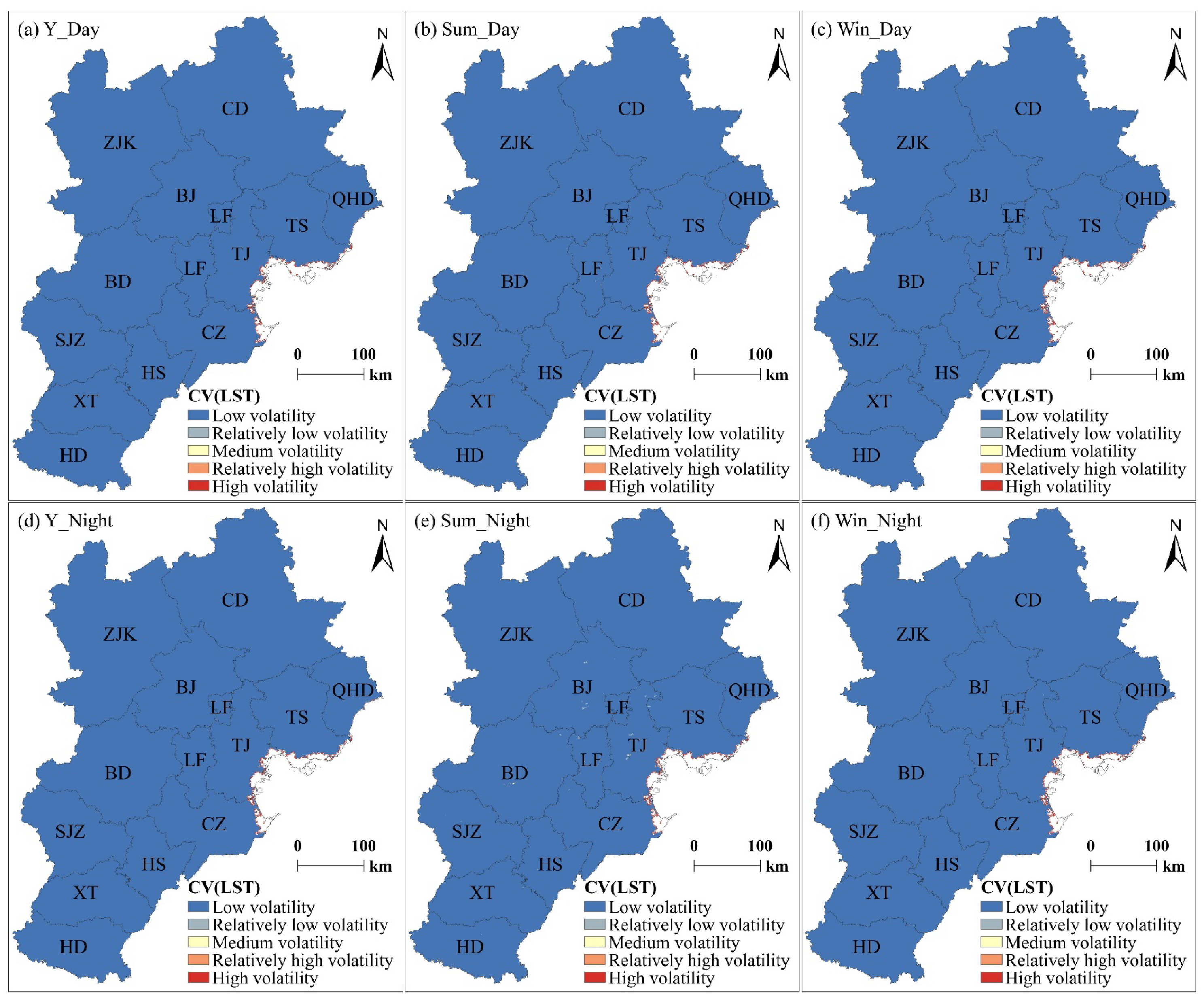
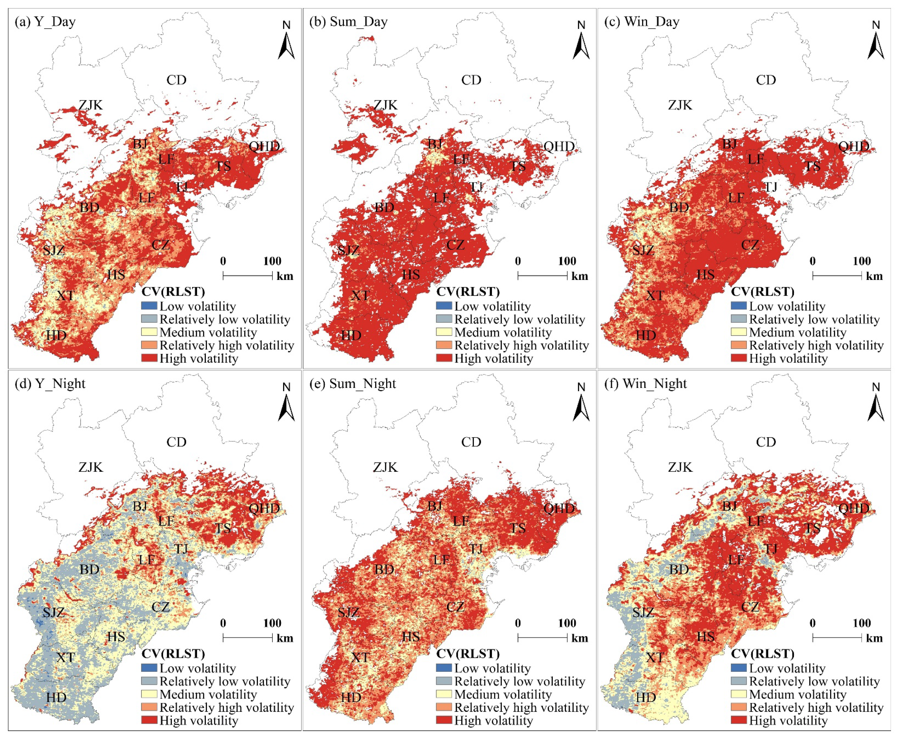


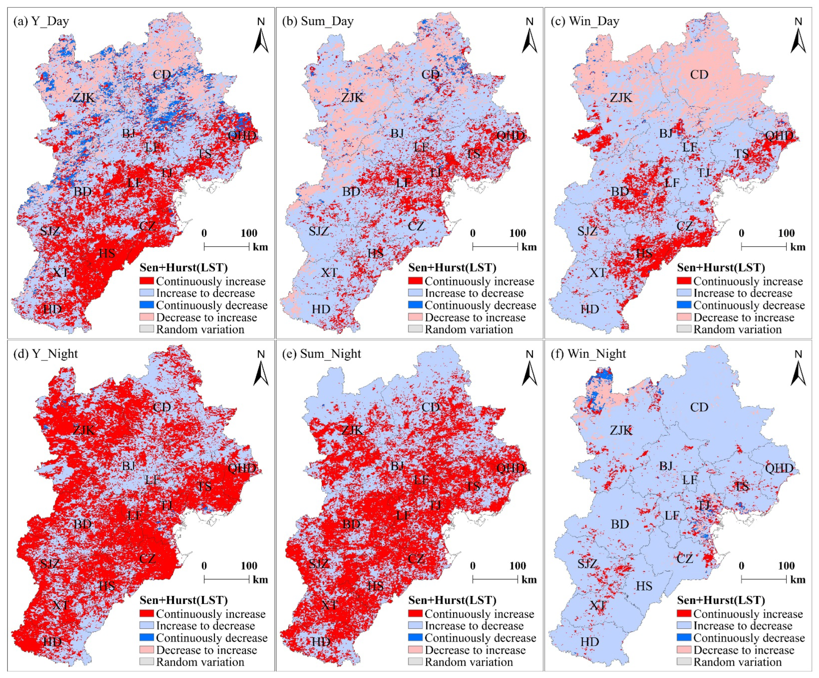

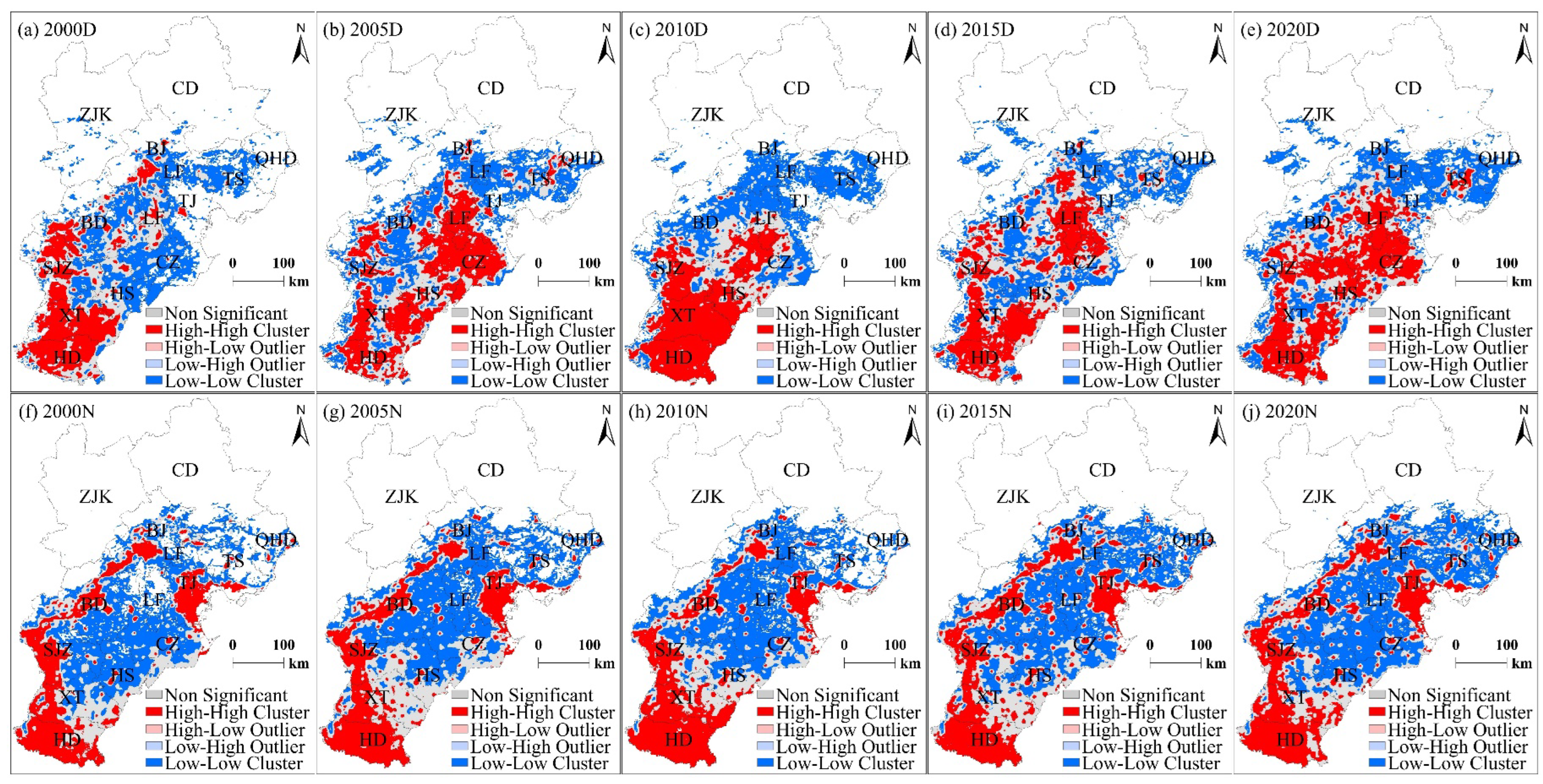

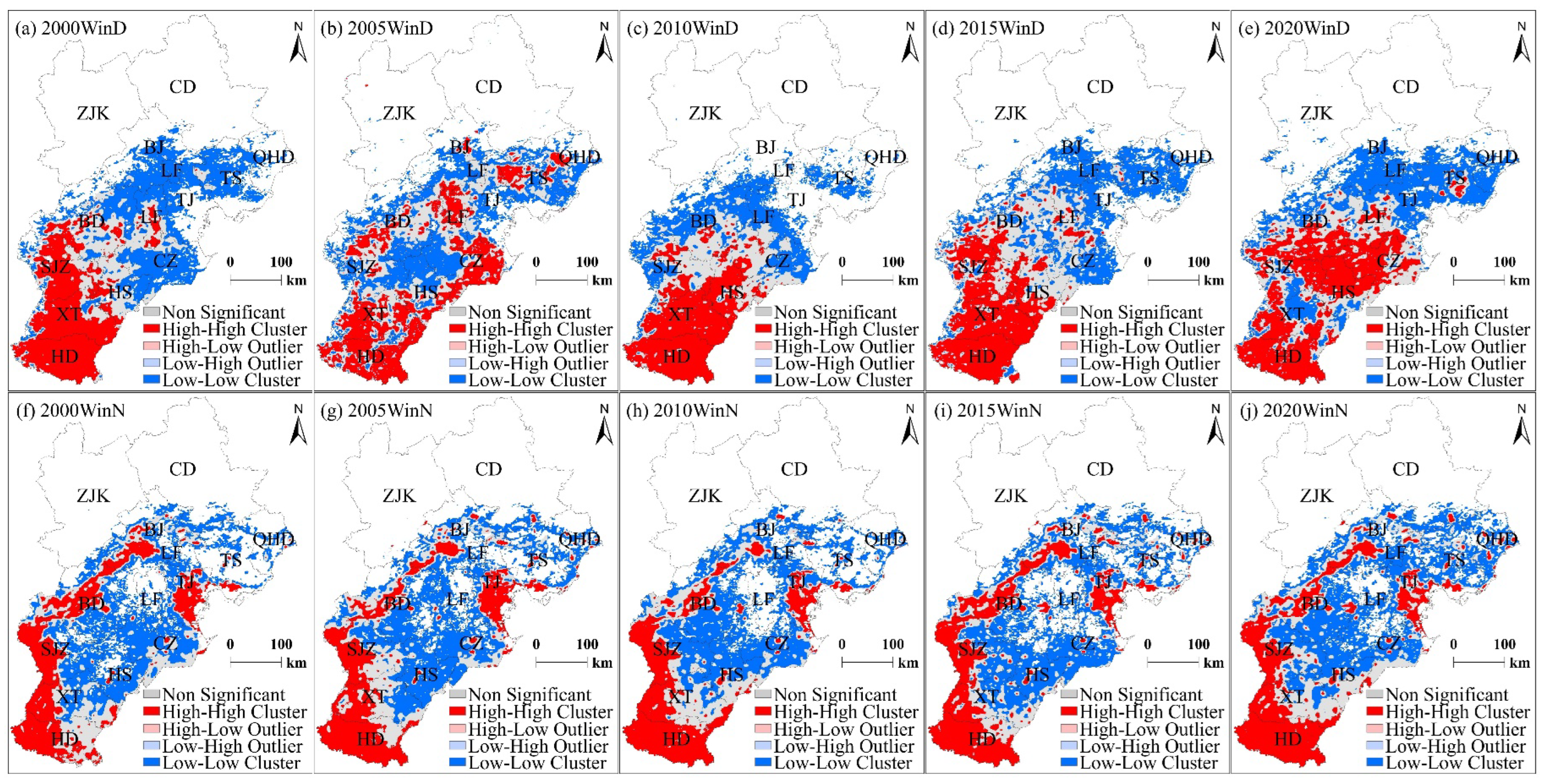
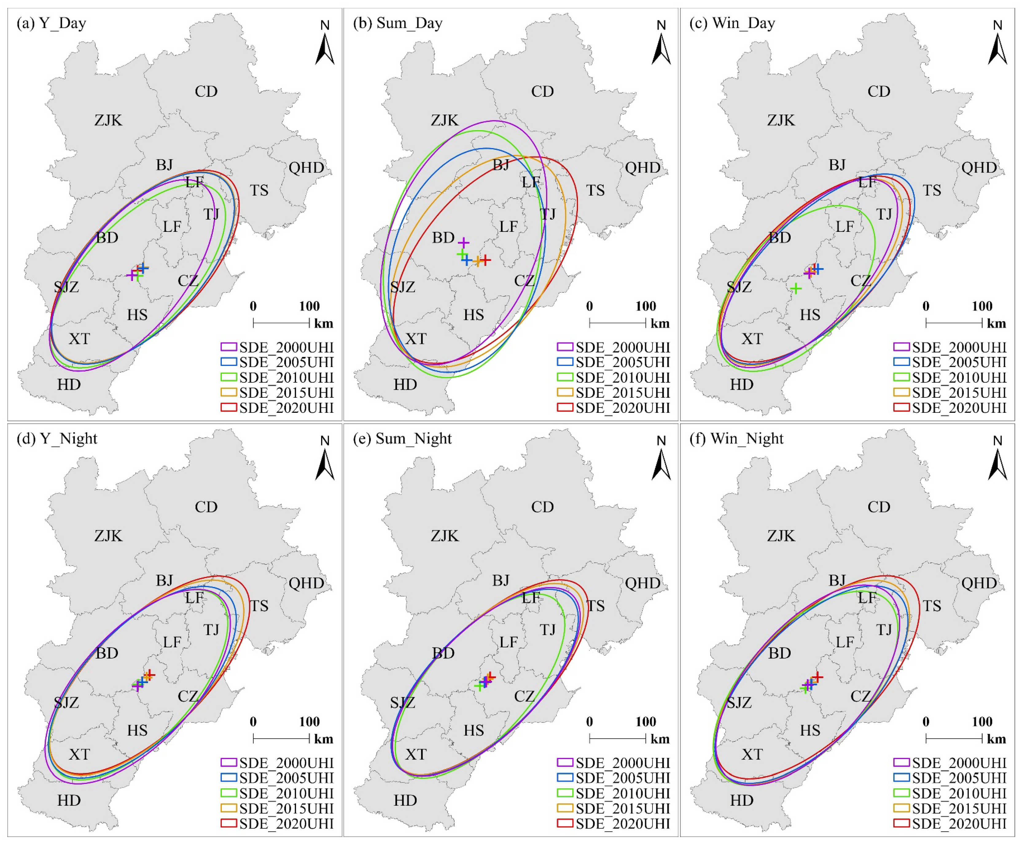
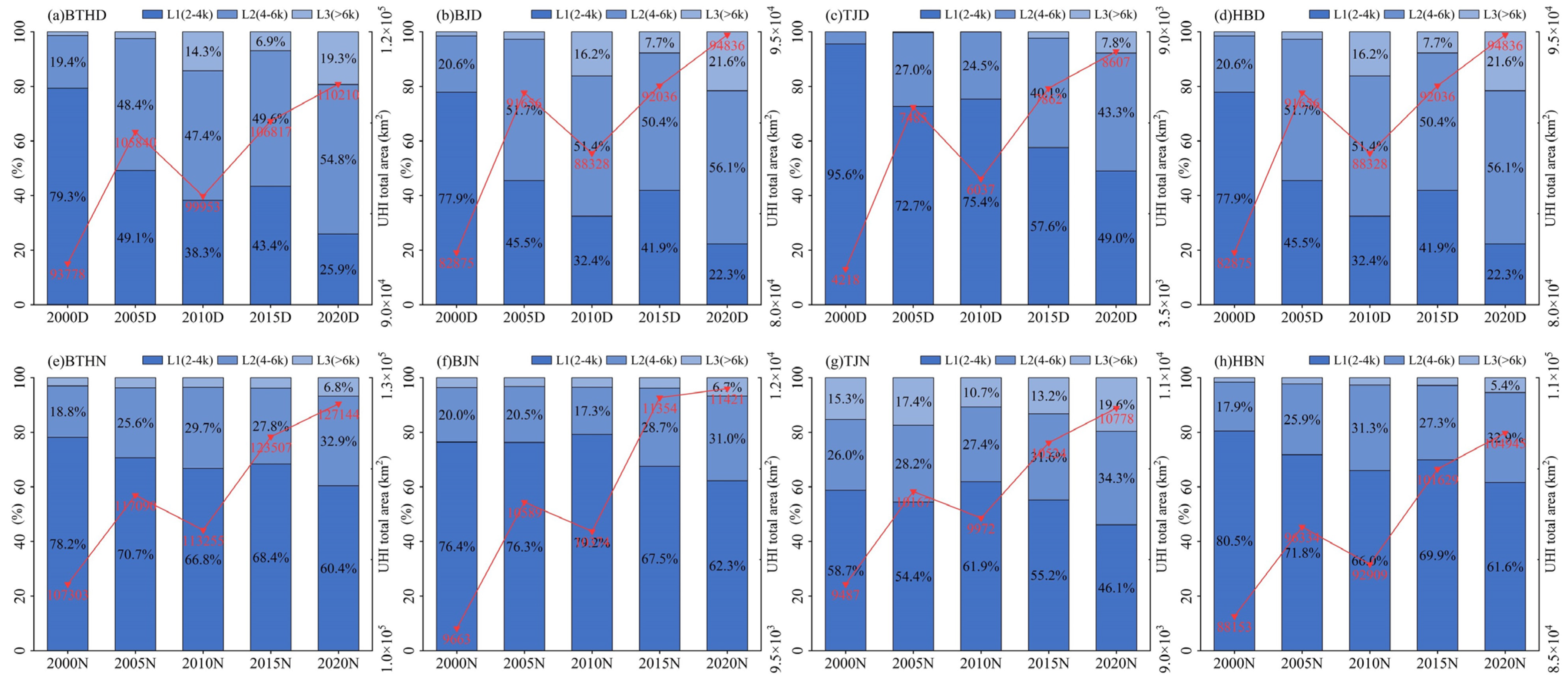
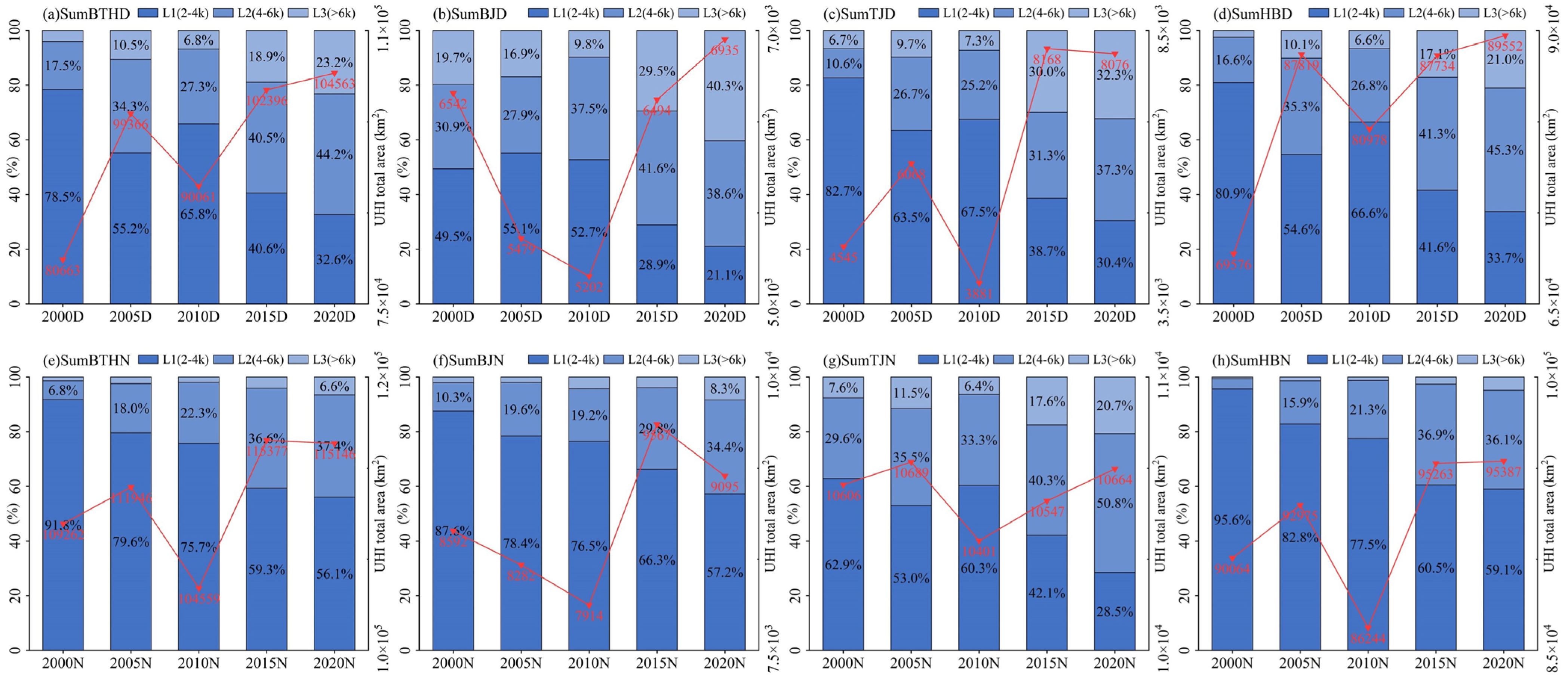
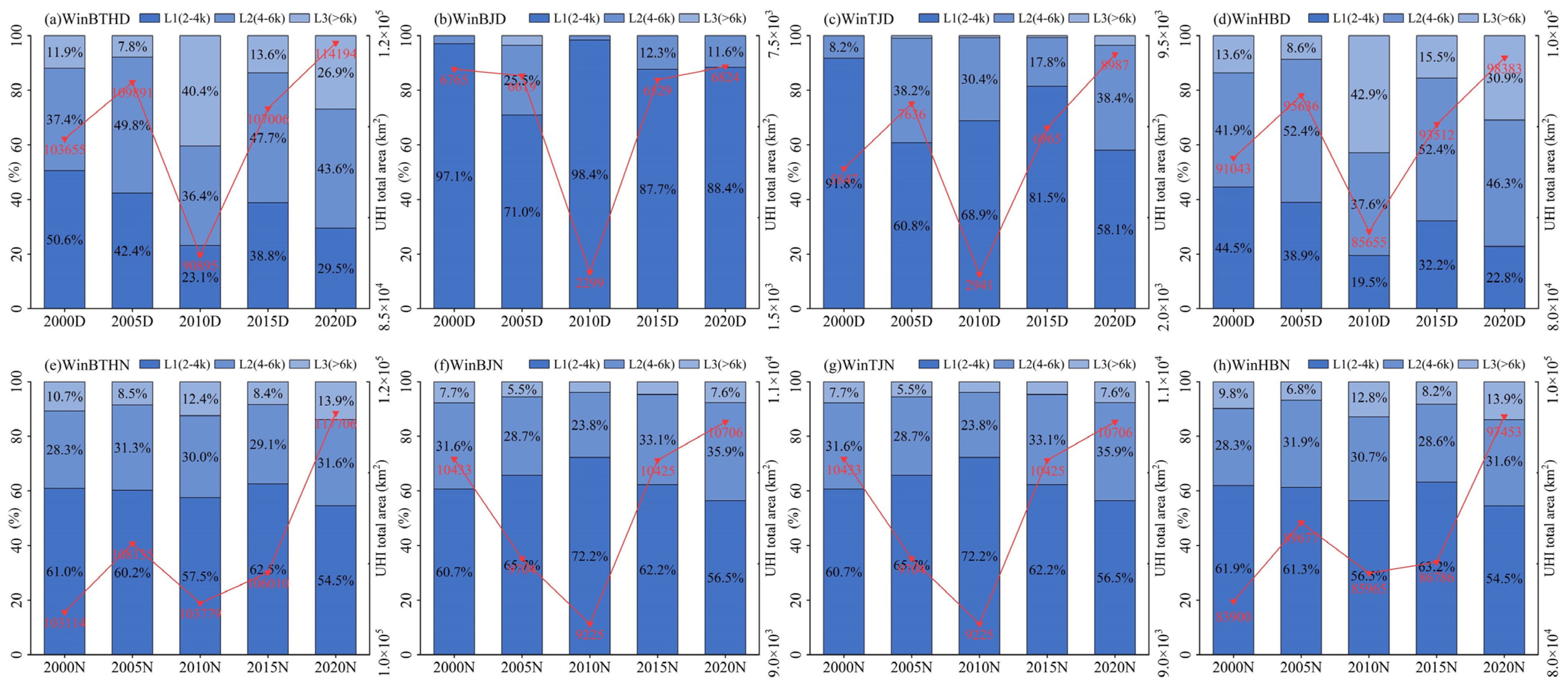
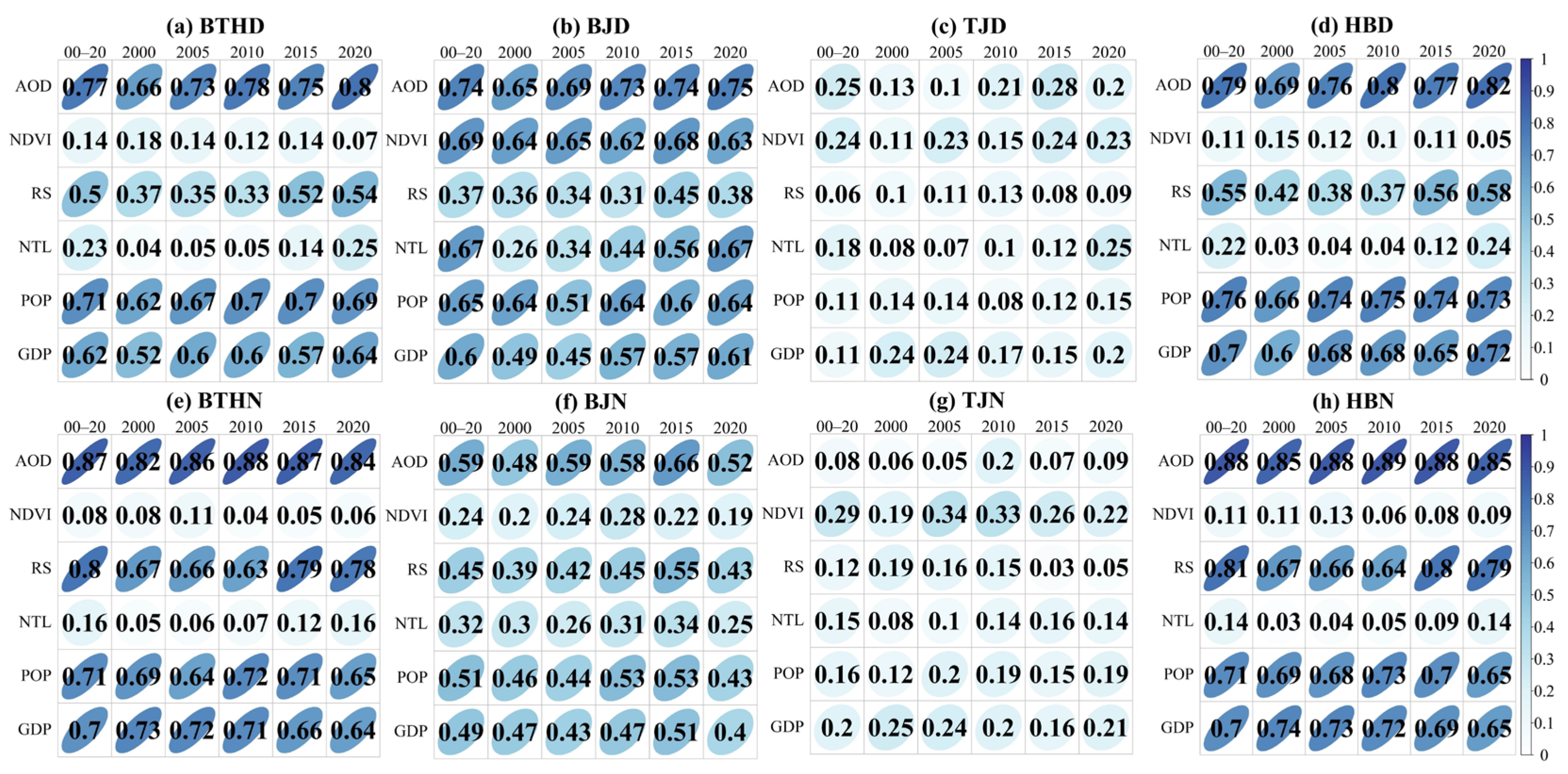
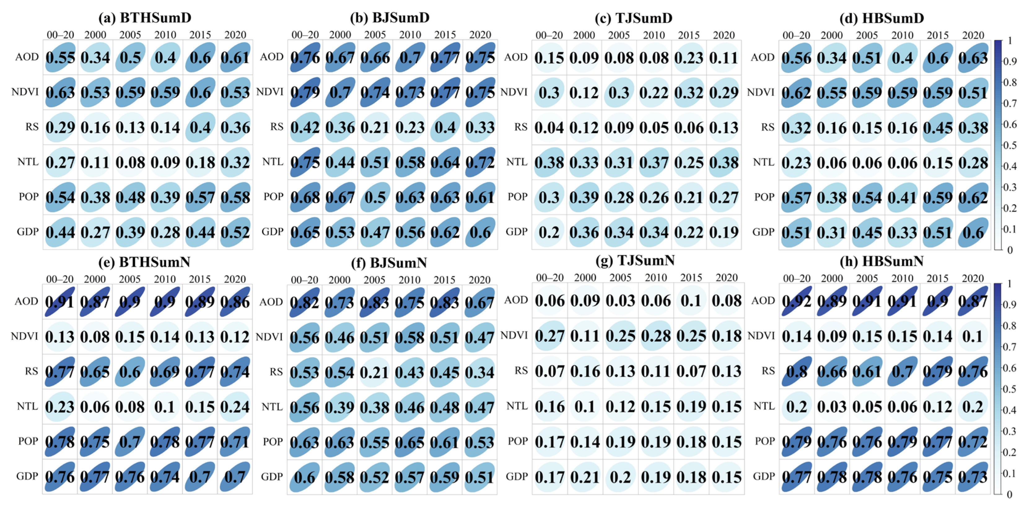
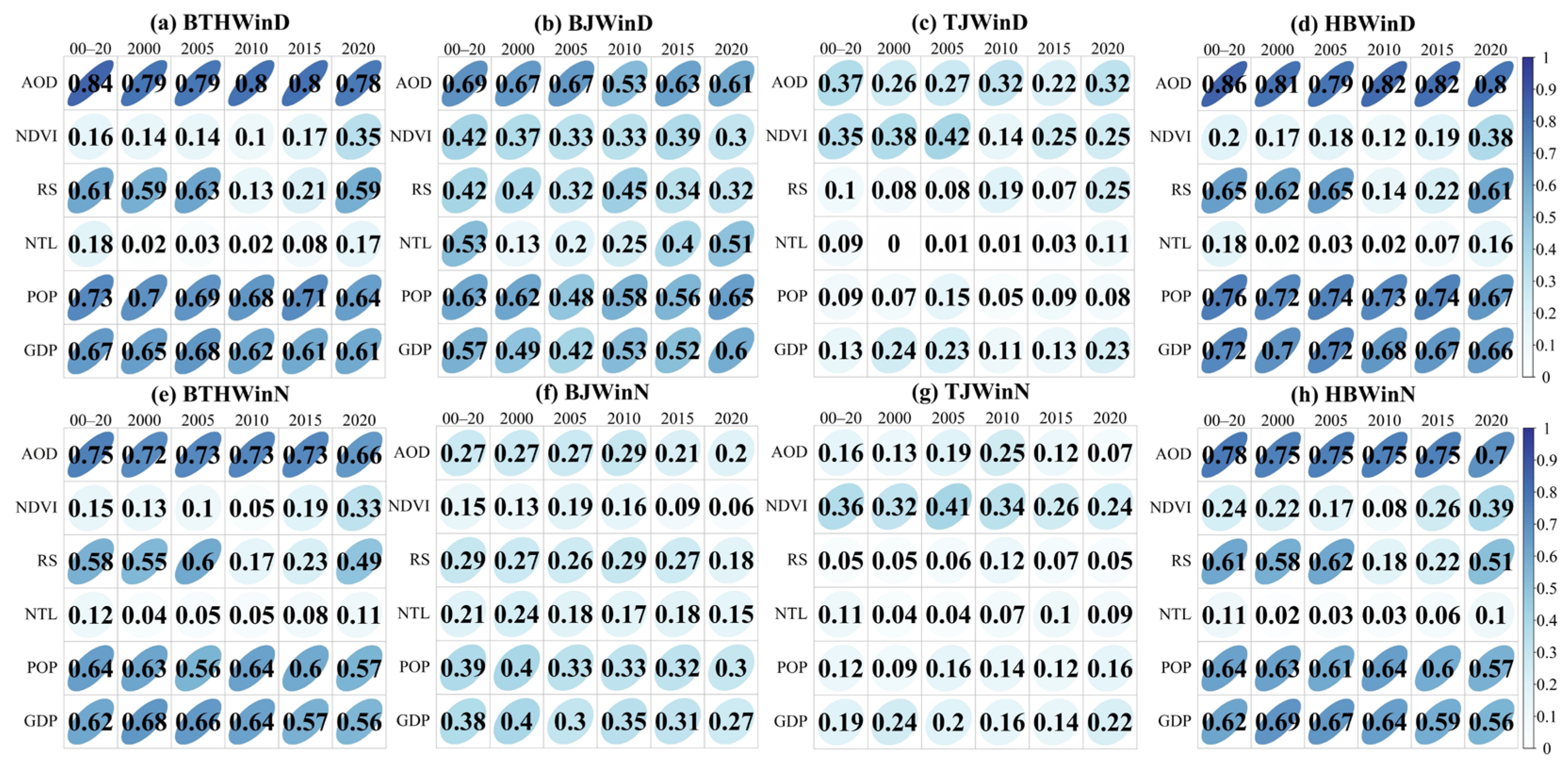
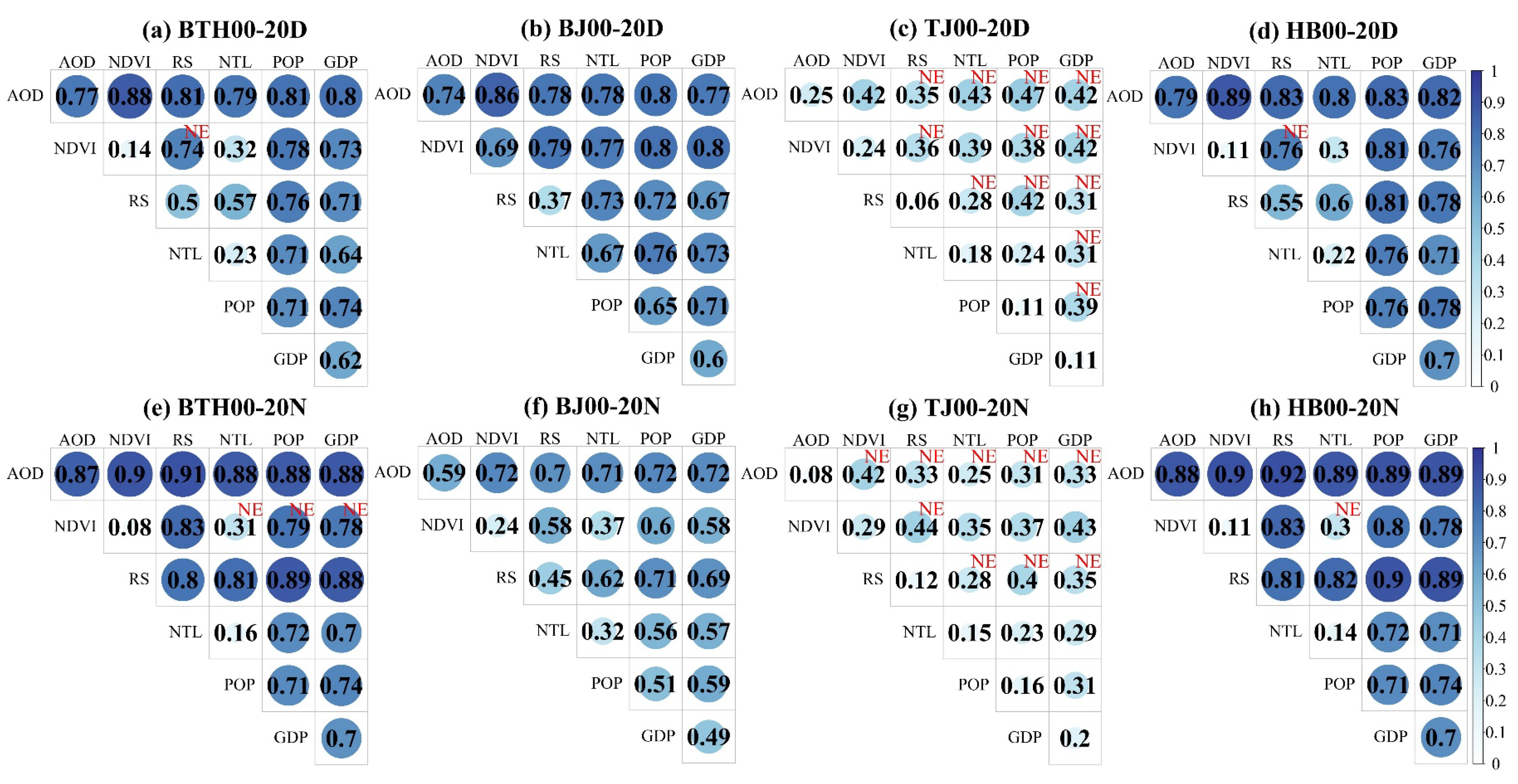

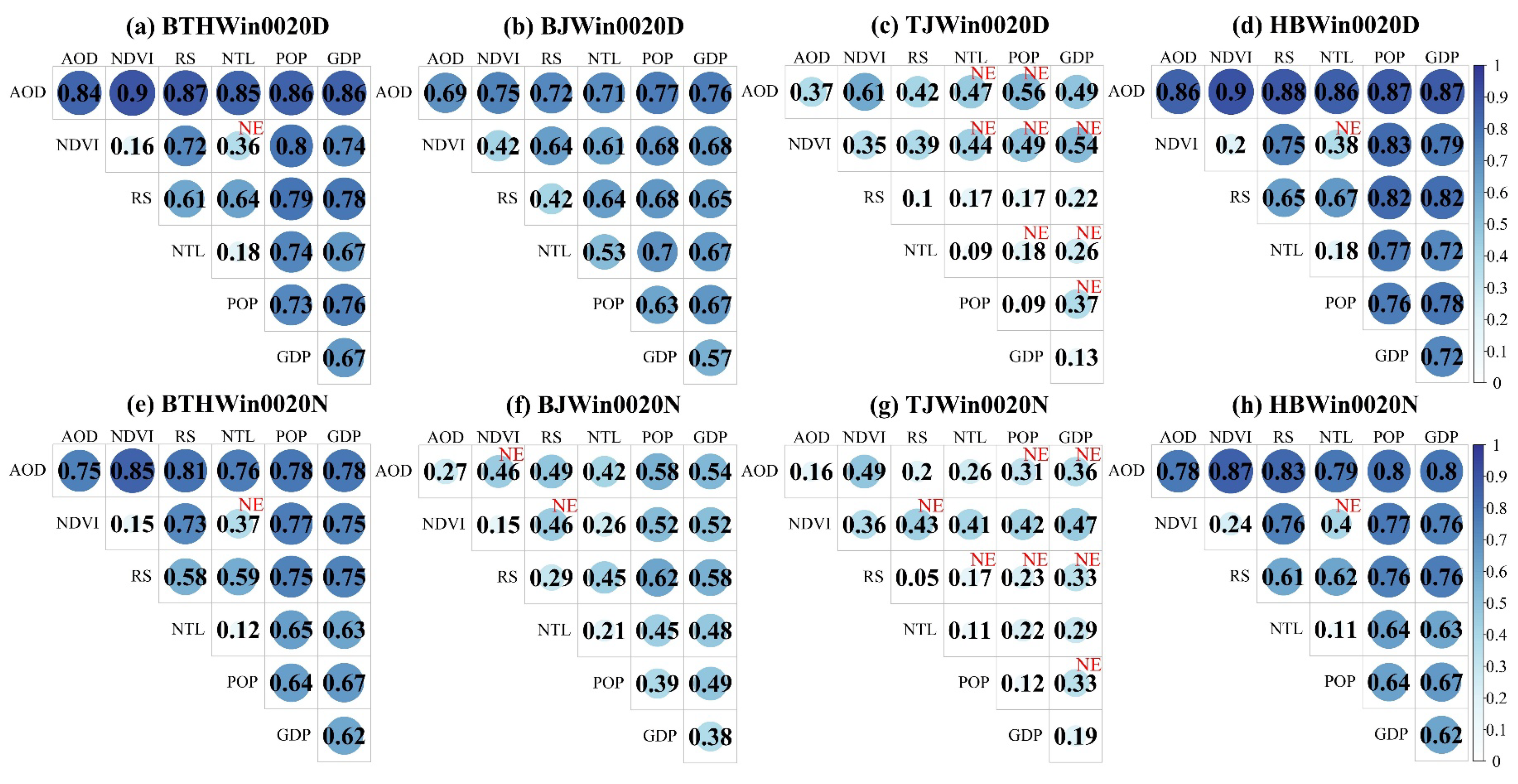
Disclaimer/Publisher’s Note: The statements, opinions and data contained in all publications are solely those of the individual author(s) and contributor(s) and not of MDPI and/or the editor(s). MDPI and/or the editor(s) disclaim responsibility for any injury to people or property resulting from any ideas, methods, instructions or products referred to in the content. |
© 2024 by the authors. Licensee MDPI, Basel, Switzerland. This article is an open access article distributed under the terms and conditions of the Creative Commons Attribution (CC BY) license (https://creativecommons.org/licenses/by/4.0/).