Abstract
The Airborne Terahertz Ice Cloud Imager (ATICI) is an airborne demonstration prototype of an ice cloud imager (ICI), which will be launched on the next generation of Fengyun satellites and plays an important role in heavy precipitation detection, typhoon, and medium-to-short-term meteorological/ocean forecasting. At present, it has 13 frequency channels covering 183–664 GHz, which are sensitive to scattering by cloud ice. This paper provides an overview of ATICI and proposes a receiving front-end design scheme using a planar mirror and a quasi-optical feed network which improves the main beam efficiency of each frequency band, with measured values better than 95.5%. It can detect factors such as ice particle size, ice water path, and ice water content in clouds by rotating the circular scanning of the antenna feed system. A high-sensitivity receiver system has been developed and tested for verification. The flight verification results show that the quasi-optical feed network subsystem works well and performs stably under vibration and temperature changes. The system sensitivity is better than 1.5 K, and the domestically produced high-frequency receiver has stable performance, which can meet the conditions of satellite applications. The ATICI performs well and meets expectations, verifying the feasibility of the Fengyun-5 ICI payload.
1. Introduction
The Airborne Terahertz Ice Cloud Imager (ATICI) is the first airborne terahertz ice cloud imager in China, jointly funded by the Xi’an Branch of the Chinese Academy of Space Technology (Xi’an) and the China Meteorological Administration (CMA). The development of ATICI is aimed at verifying the performance of future ICI (ice cloud imager) payloads mounted on Fengyun-5. An ICI contains 13 detection channels between 183 and ~664 GHz, and is a new type of payload for the detecting of macro and micro characteristics of ice and clouds, which has important applications in many aspects such as improving the accuracy of climate prediction and numerical weather prediction as well as extreme weather prediction capability in the future [1,2,3,4], and is of great significance to meet the increasing demand for climate prediction and weather forecasting from the military and civilian sectors [5].
The European Space Agency (ESA) has developed the world’s first on-board ICI, which will be launched on board the MetOp second-generation (MetOp-SG) satellites in 2025 [6,7]. China’s Fengyun V(FY-5) meteorological satellite also lists ICI as one of its main payloads. To verify the performance of such payloads, NASA, the ESA, the Met Office, and other agencies have conducted extensive technical studies and airborne detection experiments (typically the Far InfraRed Sensor for Cirrus (FIRSC) [8] and the International Submillimetre Airborne Radiometer (ISMAR)) [9,10,11]. The FIRSC Fourier transform spectrometer is used on the Proteus high-altitude aircraft and has two frequency bands covering approximately 300~1000 GHz with a detector footprint of less than 1 km, and an NEDT of about 1 K. In 1999, the FIRSC conducted a series of airborne experiments, and the results amply demonstrated that the ice-water path (IWP), size, and polarization of ice clouds are spectrally sensitive in the terahertz band. However, because the FIRSC uses cryogenic detectors, the system is not suitable for satellite-based applications. CoSSIR is an airborne compact terahertz full-power imaging radiometer developed by NASA [12], specifically designed for experimental research on ice cloud ice crystal particle scale and ice water path. The operating frequencies are selected as 183 GHz, 220 GHz, 380 GHz, 487 GHz, 664 GHz, and 874 GHz, and the receivers in each frequency band use a Schottky diode-based superheterodyne mixing detection method. All the receivers and radiometer electronics are housed in a small cylindrical scan head (21.5 cm in diameter and 28 cm in length) that is rotated by a two-axis gimbaled mechanism capable of generating a wide variety of scan profiles. This gives a nadir footprint at the surface of about 1.4 km at an ER-2 cruising altitude of 20 km. However, CoSSIR uses a feed array for direct observation and does not have a reflector antenna, making it unsuitable for spaceborne applications.
ISMAR is co-funded by the Met Office and the ESA. It first flew in 2014 and currently has seven uncooled heterodyne receivers providing 15 channels operating at 118~664 GHz, and receivers at 874 GHz are being developed by Omnisys. ISMAR is used on FAAM BAe-146 aircraft for atmospheric research, and is installed in the radiometer blister on the front port side of the aircraft, providing unobstructed upward and downward views. The ISMAR’s upward view is −40°~10°, and its downward view is −10°~55°. However, ISMAR also has shortcomings. Its footprint is not concentric circles, resulting in differences in the geographical location of the observed brightness temperature at different frequencies. Also, because ISMAR is mounted on the side of the aircraft, it has a narrow scan width. The main differences of several instruments are shown in Table 1.

Table 1.
The main differences of instruments.
The available data is too small to build accurate terahertz radiative transfer models. To improve the accuracy of ice cloud retrieval, the ATICI and ice cloud simultaneous observing instruments are used for experimental validation. The ATICI is carried on board a Cessna 550 ice cloud research aircraft (Figure 1), which can fly at altitudes of up to 10,000 km. The ATICI receiver, which operates at frequencies between 183 and 664 GHz, is mounted under the aircraft without a wave-transparent cover and uses circular scanning geometry. Therefore, ATICI has no transmission loss due to wave-transparent cover, and the downward view is −55°~55°. As ATICI uses a quasi-optical feed system rather than a receiver array, its footprints are concentric circles.
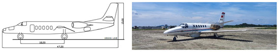
Figure 1.
Cessna 550 aircraft.
The main objectives of ATICI are as follows:
- (1)
- Optimize the system indicators for the subsequent Fengyun-5 ICI payload, laying the foundation for subsequent ICI applications.
- (2)
- Verify the performance of domestically produced high-frequency receivers and test their sensitivity.
- (3)
- Verify the performance of the 183–664 GHz quasi-optical feed network subsystem.
- (4)
- Accumulate observation data to provide support for subsequent validation of inversion algorithms.
2. Instrument Design
Based on the radiation characteristics of ice clouds, ATICI selected the highly sensitive 183–664 GHz band for detection, which contains a total of 13 detection channels. The system has been designed in an integrated manner, using a receiver front-end design scheme with a pair of plane mirror reflectors, a quasi-optical feed network, and a circular scan by rotating the plane mirror. The antenna beam is scanned in a plane perpendicular to the flight path, and the footprint on the ground is a direct one. The scanning schematic is shown in Figure 2.
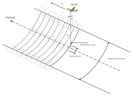
Figure 2.
Diagram of scanning method.
The flight altitude of the Cessna 550 aircraft is 10,000 m, the aircraft speed is 580 km/h, and the Earth view sampling ranges from −70° to 70°. The number of Earth observation points is 50, and the scanning step angle is 2.2°. Circular scanning is used.
ATICI proposes to use a full power type radiometer, consisting of five main functional modules: an antenna and scanning subsystem, a multi-band terahertz receiving channel, a calibration subsystem, a data acquisition and processing platform, and a control distribution display system. A schematic block diagram of the system is shown in Figure 3.
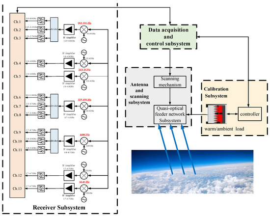
Figure 3.
ATICI interconnections schematic.
The operation of the ATICI can be described as follows: The servo controller controls the scanning mechanism, which performs circular scanning. Ground observation and calibration occur during each rotation cycle. The quasi-optical feed network separates the received signals by frequency and polarization, and then sends the signals to the receiver for mixing, amplification, filtering, and detector processing. Then, the information acquisition control and distribution unit performs information acquisition and other processing, organizes the acquired and processed telemetry data, and stores them in the ATICI’s own memory. The acquisition control and distribution unit completes the exchange of remote-control commands and telemetry status display commands with the vehicle platform.
The aperture of the reflector is 250 mm, and the antenna reflector, scanning mechanism, quasi-optical feed network, and receiver are laid out in the combined form of Figure 4. The height of the reflector center from the base plate is about 248 mm, and the height of the mounting plate of the quasi-optical feed network and receiver from the base plate is about 183 mm. The size of the calibration controller is 248 mm × 204 mm × 45 mm, and the size of the acquisition control and distribution unit envelope is 420 mm × 482 mm × 177 mm. Instruments are contained in a single package with dimensions of approximately 1.0 m × 0.55 m × 0.4 m and a weight of around 60.6 kg, Power consumption is 495 W (Figure 4). Fans are added on both sides of the reflector to prevent frosting and water vapor condensation during the flight through the clouds.
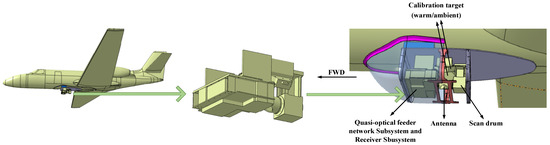
Figure 4.
Schematic of ATICI.
The advantage of the periodical calibration full power type receivers is that it does not use a Dicke switch. This means the equipment is simple and the loss caused by the Dicke switch is reduced, which helps to improve the measurement uncertainty caused by system noise. In addition, the ideal temperature measurement sensitivity is about twice as high as that of Dicke-type receivers. The gain variation error caused by the long-term operation of the periodical calibration full power type receivers can be improved by means of periodic calibrations, which were performed using ambient and warm loads.
The multi-band terahertz receiver includes three parts: a harmonic mixer, a local oscillation link, and an IF amplifier circuit and signal detector for each frequency band. This allows the superheterodyne detection of terahertz radiation through harmonic mixing. The ATICI technology scheme is shown in Table 2.
Table 2.
ATICI technology scheme.
In the Earth observation system, clouds are one of the most important and difficult meteorological elements to determine, especially ice clouds in the upper troposphere, which have a high coverage of the Earth’s surface and an important impact on the Earth’s energy balance, climate change, and weather evolution. The size of ice crystals in ice clouds is generally from a few to several thousand microns, and the microwave millimeter wave used in traditional satellite-based remote sensing systems is insensitive to ice clouds, while infrared/visible light has poor penetration to ice clouds, and neither of them can achieve effective detection. The wavelength of terahertz wave (100 GHz–10 THz), which is in the middle of microwave/millimeter wave and infrared/visible light, is closer to the size of the main particles in ice clouds. Therefore, the brightness temperature of the terahertz band is very sensitive to the main detection elements, such as the ice cloud, ice water path, and ice crystal size. This band has been considered the best frequency band for ice cloud detection. The ice crystal size parameter , = 0.4 for ice crystals in ice clouds, and the ATICI channel frequency range is from 183 to 664 GHz, so the detectable ice crystal size can cover 50~200 μm. The shape, size, and distribution of ice particles in ice clouds vary, and their formation is related to the temperature and humidity at that time. According to the measurement results, ice clouds contain a considerable number of non-spherical ice particles, with larger ice particle sizes at higher temperatures. Generally speaking, in tropical regions, ice clouds in the atmosphere are mostly sheet-shaped particles, while in mid-to-high latitudes, they are mostly columnar ice particles. The size of ice particles is mostly concentrated in the range of 25–400 μm. The ATICI can detect most ice particle sizes.
The three channels at 183.31 GHz are used to detect water in the vapor profile. The 243.2 GHz channel is used to detect ice clouds and cirrus, the three channels at 325.15 GHz can be used to detect ice cloud effective radius, and the three channels at 448 GHz and 664 GHz are used to detect the ice water path. All channels have dual bands, which improves the sensitivity of the instrument and suppresses the effect of frequency drift on detection results. The window channels 243.2 GHz and 664 GHz have two receivers to measure the double polarization, which can eliminate the interference of changes in surface or lower-middle cloud radiation characteristics to ice cloud detection, and also provides information about the ice cloud, cirrus, and ice water path [2].
The main purpose of the ATICI instrument is to perform ice cloud retrieval. The ATICI will provide information on the average height of the ice cloud, the ice water path, and the ice cloud’s effective radius. In addition, the ATICI will also provide water vapor profile measurement capability [13]. A full overview of the ATICI’s channel parameters is given in Table 3.
Table 3.
Main specifications of the ATICI.
3. Sensor Description
3.1. Calibration Subsystem
The essence of the ATICI calibration is to determine the output voltage of the radiometer in relation to the apparent temperature of the antenna. The linear relationship between the input and output of the radiometer can be determined from measurements of two loads with known brightness temperatures, so that at least two loads with known brightness temperatures are required for the radiometer in-orbit calibration. The radiometric brightness temperature of the calibration loads is at the two ends of the temperature range, and the brightness temperature difference between them is increased as much as possible, which will help to improve the calibration accuracy.
If the linearity of the radiometer receiver conditions can be met, the receiver output voltage and input brightness temperature will have a linear relationship. This means the relationship between the radiometer output voltage and input brightness temperature can be expressed as follows:
As soon as two known input brightness temperatures are provided, the relationship between the output voltage of the radiometer and the input brightness temperature can be determined from its output, i.e., the constants a and b of the linear equation can be determined.
For the flight calibration scheme, the low-temperature calibration load uses an ambient load with the same ambient temperature, which is about 220 K at an altitude of 12,000 m. The high-temperature calibration load uses a standard radiation black load (Figure 5) with a radiation brightness temperature heated to about 330 K. The warm load is a microwave-absorbing material with a pyramidal structure, and the control of physical temperature is realized by an electronic thin film heater. In order to improve the accuracy of physical temperature measurement, a set of platinum resistance thermometers (PRTs) was mounted in the warm load. Several platinum resistors are placed in the center tip bottom, center tip top, edge tip bottom, edge tip top, and other positions of the tip split within the warm load, and the physical temperature of the warm load is calculated based on the actual measured values of these temperature measurement points and the thermal conductivity and temperature gradient of the warm load. The stability of the warm load is less than 0.15 K and the accuracy of the warm load temperature is less than 0.1 K. The load emissivity is 0.999.
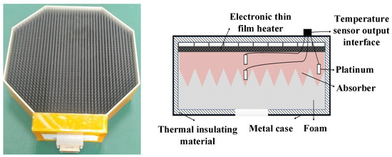
Figure 5.
Standard radiation black load.
For radiometers to match the system output voltage, and for the antenna’s apparent temperature to correspond with and achieve quantitative measurement, the system must be calibrated periodically. This also reduces the impact of the receiver gain changes. The terahertz ice cloud sky bottom detector calibration will be used with the end-to-end two-point mouth surface calibration method in order to calibrate the measurement channel system parameters. The flight calibration schematic is shown in Figure 6. The ambient load view sampling ranges from 216.2° to 233.8°, with eight observation points, and the warm load view sampling ranges from 126.2° to ~143.8°, with eight observation points.
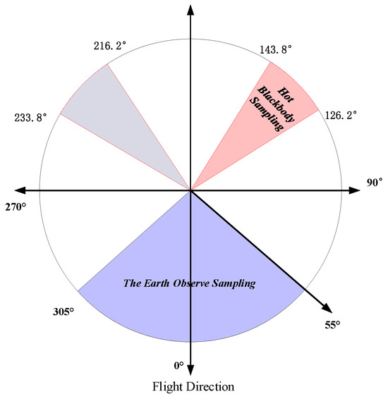
Figure 6.
Flight calibration schematic.
In the two-point calibration type microwave radiometer, the received power of the black body is usually considered to be linearly related to its temperature, and according to Planck’s radiation law, a blackbody radiates uniformly in all directions with a power P given by
where is in ; is Plank’s constant (); is Boltzmann’s constant (); is frequency (Hz); is the blackbody’s absolute temperature (K); and c is the velocity of light in vacuum ().
The Rayleigh–Jeans approximation is very useful in the microwave region: it is mathematically simpler than Planck’s law and yet its fractional deviation from Planck’s exact expression is less than 1% if
The above inequalities will hold if GHz. At 300 GHz, the fractional deviation is about 3%. However, at the maximum frequency used by ATICI, the Rayleigh–Jeans approximation is deviation and Wien’s law is required. For terahertz, . So Equation (2) can be simplified as
3.2. Quasi-Optical Feed Network Subsystem
The existing airborne and satellite-based ice cloud imager design solutions (ICI and ISMAR) both adopt the design of feed and signal separation by integrating the feed array and the receive front-end. This solution faces the problem of difficult heat dissipation in the feed array and the receive front-end, which in turn affects the detector detection accuracy and other key performances. The relevant development units have recognized this challenge and included it in their next work plan.
The new quasi-optical feed network scheme can overcome the deficiencies of the existing terahertz ice cloud detector system. This approach utilizes a pair of plane mirrors and a quasi-optical feed network [14] in the receiving front-end design scheme to achieve the observation of ice and water particles in clouds. First, it solves the space environment adaptability problem of the feed array and receiving front-end heat dissipation difficulties in the existing system. Second, it improves the main beam efficiency of each frequency band, and then improves the detection accuracy of the detector. Third, it improves the design flexibility and engineering realizability of the detector system.
The scanning mechanism drives the detection head to carry out 360° scanning, and the scanning imaging is carried out at −55°~55° in each rotation cycle. The polarization line grid is used to polarize and separate the terahertz signal received by the antenna. The H-polarized wave is divided into high and low-frequency branches by frequency-selective surfaces [15,16,17] FSS#1. The high-frequency branch is separated into 664 GHz polarized detection, and the low-frequency branch is separated into 243 GHz. FSS#2 is divided into two branches of high and low frequency, and the high-frequency branch is separated into a 664 GHz detection branch while the low-frequency branch is separated into 448 GHz, 325 GHz, 243 GHz, and 183 GHz branches by FSS#3, FSS#4, and FSS#5 in turn. The multi-band terahertz reception adopts the direct mixing and double-band reception method, in which the RF signal from the frequency divider to the receiver is mixed directly, followed by IF filtering, amplification, and square-law detection to obtain the final signal.
The entire quasi-optical feed network has a compact size envelope of about 400 × 400 mm. The structure of a quasi-optical feed network with multi-band receivers is schematically shown in Figure 7.
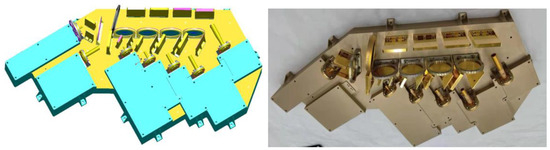
Figure 7.
Quasi-optical feed network and receiver physical diagram and schematic diagram.
The 183 GHz band is the last level of frequency separation, so the beam transmission path in this band will be the longest. When the output beam parameters of 183 GHz frequency band are determined, the output beam parameters of other frequency bands can be determined. The finalized output beam parameters of the quasi-optical feed network are shown in Table 4.
Table 4.
Main specifications of the quasi-optical feed network.
- Frequency-selective surface
The quasi-optical feed network uses a frequency-selective surface in the form of high-frequency transmission and low-frequency reflection, with a total of five frequency-selective surfaces. Its resonant structure unit size is small and requires high processing accuracy; however, its reflection characteristics at low frequencies are particularly good.
For the choice of frequency-selective surface cell form, an all-metal, non-dielectric support double-layer structure has the advantages of wide bandwidth and small insertion loss, so choose the double-layer all-metal type of frequency selection surface. A “C” type structure is selected for the cell, and the arrangement of the cell shapes is shown in Figure 8.
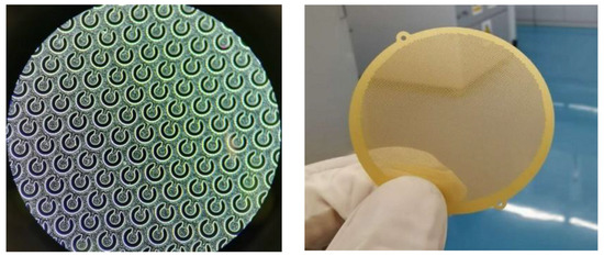
Figure 8.
Frequency selection surface.
For the “C” structure frequency selection surface, the electric field direction of the TE wave (V polarization) is perpendicular to the short side of “C”, and the electric field direction of the TM wave (H polarization) is parallel to the short side of “C”. The simulation schematic is shown in Figure 9. The characteristics of each frequency selection surface are summarized in Table 5.
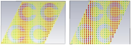
Figure 9.
Simulation diagram of TM wave (H polarization) and TE wave (V polarization) for “C” type unit.
Table 5.
The characteristics of each frequency selection surface.
FFS#1 achieves the separation of TE waves (V-polarization), where the angle between the incident and reflected beams is 60°, the passband is 664 GHz, and the reflected bands are 448 GHz, 325 GHz, 243 GHz, and 183 GHz. The transmission loss of the 664 GHz frequency within the ±7 GHz bandwidth range is less than 0.3 dB (with an incidence angle range of 30 ± 5°), and the reflection loss of the other four frequencies within the operating bandwidth range is less than 0.05 dB.
- 2.
- Polarization Line Grids
The main function of the polarization line grating is to separate the line polarization plane waves in both vertical and horizontal directions. Its structure is a substrate-free type, consisting of thin metal wires uniformly wound on a rectangular frame to form a grating structure. The structure is shown in Figure 10.
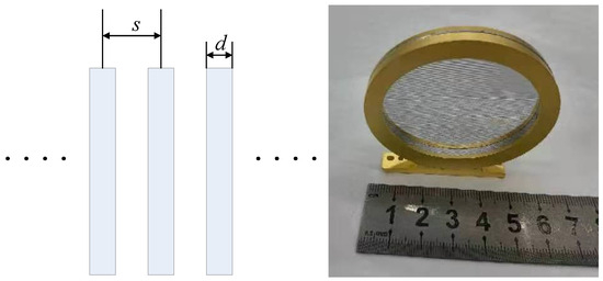
Figure 10.
Substrate free metal fine wire grid structure.
The spacing between the grid intervals is denoted by “s” and the diameter of the fine metal wire is denoted by “d”. The reflection and transmission characteristics can be changed by adjusting the diameter and spacing of the metal filaments in the operating frequency. The unit simulation cell model of the polarized wire grid is shown in Figure 11.
Figure 11.
Substrate free metal fine wire grid structure.
The incident wave has an angle of incidence of φ = 0°, θ = 45°, The TE wave (V polarization) has an electric field direction parallel to the y-axis, and the TM wave (H polarization) has an electric field direction parallel to the x-axis, and is totally reflective. The frequency characteristics of the vertically polarized wave are shown in Figure 12.
Figure 12.
Reflection and transmission characteristics of vertically polarized waves by polarization line gratings (a,b).
From the simulation results, the transmittance transmission loss of the polarized grid network to the vertical polarized wave is less than 0.1 dB in the whole operating frequency band. The frequency characteristics of the parallel polarized wave are shown in Figure 13.
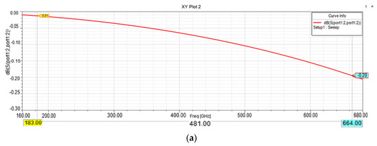
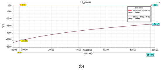
Figure 13.
Reflection and transmission characteristics of horizontally polarized waves by polarization line gratings (a,b).
From the simulation results, the reflection loss of the polarized grid network to the parallel polarized wave is less than 0.2 dB in the whole operating frequency band. The characteristics of polarized wire grids are summarized in Table 6.
Table 6.
The characteristics of polarization line grid.
- 3.
- Feed Horn Antenna
The quasi-optical feed network is designed based on Gaussian beam theory, and the ideal Gaussian beam should be a radiation beam with no cross-polarization and ultra-low sub-petal level. Therefore, the horn antenna in a quasi-optical feed network adopts a corrugated horn antenna, which requires a high Gaussian fundamental mode coupling efficiency of above 99%. The corrugated horn antenna has a corrugated inner wall with a sin/parallel line curve form. The physical and model schematic diagram of the corrugated horn is shown in Figure 14.
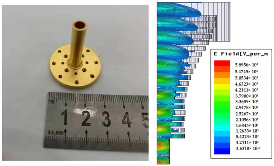
Figure 14.
The physical and model schematic diagram of the corrugated horn.
The biggest difficulty with corrugated horn antennae in the terahertz band is the processing and manufacturing technology they use. Considering the extremely high precision requirements for machining, electroforming is required for product processing. Electroforming is used to make metal products by electrodepositing metal on the surface of the core mold and then separating the electrodeposited metal layer from the core mold. The corrugated horn antenna characteristics are summarized in Table 7.
Table 7.
The characteristics of corrugated horn antenna.
The radiation direction diagrams of the E and H sides of the 664 GHz feedhorn antenna are shown in Figure 15.
Figure 15.
E-plane (a) and H-plane (b) radiation pattern of 664 GHz horn.
3.3. Receiver Subsystem
The receiver subsystem is divided into three parts: the terahertz front-end, the IF channel, and the local oscillator (LO). The main function of the terahertz front-end is to mix the input double-sideband signal with a certain bandwidth to zero IF, and to achieve this function while minimizing the noise temperature of the receiver. The terahertz receiver channel consists of a mixer, a LO, an IF low-noise amplifier (LNA), an IF filter, and a detector. The DC signal after the detector is amplified and biased and then output. The terahertz mixer is usually used as the front end of the receiver, and its performance has the greatest impact on the overall receiver performance.
The LO circuit locks the input reference signal between 2000 MHz and 4000 MHz through a comb spectrum generator and a digital mixing ring circuit, and then achieves the local oscillator signal in the Ku frequency band through an eight-fold frequency circuit. The frequency source adopts MCM technology to package the bare chip and packaged device in the same shell. The schematic diagram of 183 GHz and 664 GHz receivers is shown in Figure 16.
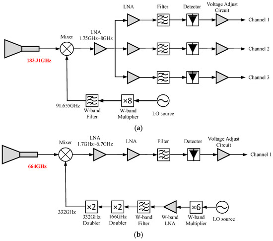
Figure 16.
Schematic of the 183 GHz (a) and 664 GHz (b) receivers on ATICI.
The structure of the receiver is a vertical assembly of three box bodies, with a fixed bottom plate at the bottom and a pull rod fastening at the top. The power supply of the three box bodies is interconnected through a PCB in the side box body. The PCB also contains the gain control circuit of the temperature compensation circuit of the entire machine. The interconnection of local oscillator signals and broadband intermediate frequency signals is achieved through semi-steel cables. The 664 GHz receiver is shown in Figure 17.
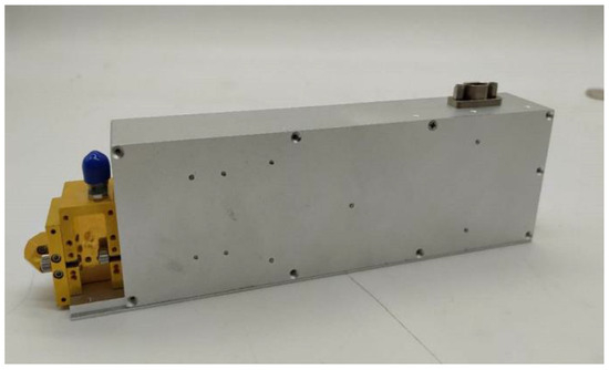
Figure 17.
Structure diagram of 664 GHz receiver.
3.3.1. Front-End Design
The terahertz RF front-end module mainly includes a mixer and a frequency multiplier. The mixer uses a Schottky barrier diode as a nonlinear device, which has the characteristics of low noise, large bandwidth, stable operation, and high cut-off frequency. By reverse paralleling two Schottky diodes, good harmonic mixing characteristics can be obtained. By reducing the local oscillator noise passband, the noise coefficient can be reduced, and it has the ability to resist reverse peak voltage. The 664 GHz harmonic mixer is shown in Figure 18.
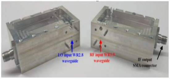
Figure 18.
The 664 GHz harmonic mixer.
The bilateral frequency conversion loss test results of the 664 GHz harmonic mixer are shown in Figure 19.
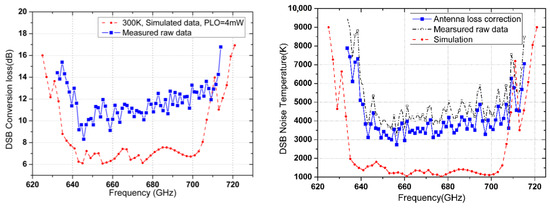
Figure 19.
The 664 GHz harmonic mixer.
Based on the test results of the 664 GHz harmonic mixer, it was found that the 0.67 THz harmonic mixer has a minimum noise temperature of 3293 K at an RF frequency of 656.4 GHz, and a double-band frequency conversion loss of −11.3 dB. At the same time, the response range of the 0.67 THz mixer is 640 GHz~710 GHz, which is greater than 70 GHz. The double-band noise temperature is between 3200 and 7000 K, and the double-band frequency conversion loss is 10–14 dB.
The frequency multiplier uses a waveguide cavity and quartz substrate to shield the microstrip. The drive signal is input by the waveguide microstrip probe and fed to the Schottky varactor diode via the microstrip transmission line. The frequency multiplier output signal is fed into the output waveguide by the microstrip probe. In order to suppress the leakage of the harmonic output to the input port, the frequency multiplier includes a harmonic suppression low-pass filter. In order to improve the efficiency of the frequency multiplier, impedance-matching structures are designed at the input and output ends of the varactor. As the local oscillator frequency multiplier in the front end of the 664 GHz receiver, the output power of the 330 GHz triple frequency multiplier needs to be greater than 5 mV. The output power of the previous 110 GHz frequency multiplier, after two-way synthesis technology processing, is 150~200 mV. Therefore, the frequency multiplication efficiency of the 330 GHz triple frequency multiplier needs to be greater than 3%. The structural design diagram of the 330 GHz frequency multiplier is shown in Figure 20. The test results are shown in Figure 21.
Figure 20.
Structural design diagram of a 330 GHz band triple frequency converter.
Figure 21.
Test Results of 330 GHz Band Tripler.
From the test results of the 330 GHz Frequency multiplier, the output power of the Frequency multiplier is more than 4~5 mV within the operating frequency range, which meets the local oscillator power of driving the 664 GHz mixer.
The 664 GHz receiver RF front-end in ATICI mainly includes a V-band triple Frequency multiplier, V-band filter, V-band amplifier, 110 GHz double frequency multiplier, 330 GHz triple frequency multiplier, and a 664 GHz mixer. The RF signal is doubled 18 times to 1/2 of the RF frequency, and the V-band filter filters out other harmonic signals to ensure good purity. The RF front-end block diagram of the 664 GHz receiver as shown in Figure 22.
Figure 22.
664 GHz receiving front-end block diagram.
The noise temperature at the front end of the receiver is shown in Table 8. As there is no low-noise amplifier above 243 GHz, the noise temperature of the receiver is relatively high.
Table 8.
Receiver front-end noise temperature.
3.3.2. Back-End Design
The back-end part of the receiver mainly performs low noise amplification, power division, filtering, and demodulation processing on the broadband intermediate frequency signal. The DC signal after demodulation is amplified and biased before being output. An electrically adjustable attenuator is added to the intermediate frequency part of the receiver to achieve temperature compensation. The RF chain adopts MCM technology, and all circuits are implemented through bare chips, packaged in a unified shell. To achieve cavity isolation and electromagnetic shielding, the RF chain adopts independent cavity separation, and the cavities will be vertically interconnected to achieve signal transmission. The schematic diagram of the receiver back-end is shown in Figure 23.
Figure 23.
Receiver back-end schematic diagram.
3.3.3. Frequency Source Design
The design principles of the five frequency sources are the same. The output frequency of the 664 GHz receiver frequency source module is 18.444 GHz, which serves as the local oscillator signal and is powered by the power supply in the entire machine. An external reference source is used to provide the reference signal, and the required local oscillator signal is output through frequency synthesis and transformation.
The 664 GHz receiver frequency source module includes the phase detector, voltage regulator, loop filter, VCO, frequency doubling, filter, and other devices. Figure 24 shows the schematic diagram of the 18.444 GHz digital loop circuit.
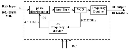
Figure 24.
Principle Composition Block Diagram of 18.444 GHz Digital Loop Circuit.
3.3.4. Sensitivity
Temperature measurement sensitivity is an important technical index of the ATICI receiver, which is defined as the minimum detectable temperature change of the input of the Radiometer receiver. The sensitivity of temperature measurement mainly depends on the noise coefficient of the high-frequency receiver and the gain stability of the receiving channel. Temperature measurement sensitivity () can be calculated by the following equation:
is the noise temperature, ; is the noise temperature of the receiver; is the loss of other components before the low noise amplifier (including antenna receiving efficiency, quasi-optical feed network loss, insertion loss of the connecting waveguide, etc.); is the bandwidth (3 dB); is the integration time, which is determined according to the system requirements and scanning cycle; represents the effect of A/D transformation, which can be ignored in 14-bit conversion; and the short-term gain instability of the channel is . The temperature measurement sensitivity is shown in Table 9.
Table 9.
Sensitivity analysis results of ATICI.
3.4. Data Acquisition (DAQ) and Control Subsystem
The data acquisition and control platform includes a data acquisition unit and a control distribution unit. The signal acquisition unit receives the output signal of each channel of the system differentially, and the received signal is amplified by an amplifier circuit with controllable gain and compensation. Then, the control circuit performs analog-to-digital conversion on the signal, and the result is sent to the ATICI system control and signal processing equipment through the universal asynchronous serial interface circuit. The result is sent to the ATICI system control and signal processing equipment through the universal asynchronous serial interface. The control parameters of the channels are also obtained through the universal asynchronous serial interface to control the compensation of the amplification circuit and to control the gain of the amplification circuit.
The control distribution system is divided into four parts according to the functional modules: the secondary power module, remote control circuit, telemetry circuit, and control circuit.
The data acquisition and control platform controls the ATICI’s working status and the exchange of information such as remote sensing, telemetry, and remote control to the outside world. It processes multi-channel remote sensing data using two-point calibration to obtain the terahertz radiation brightness temperature of the lower atmosphere in the troposphere after the scattering of ice clouds. It also calculates the multi-channel terahertz radiation brightness temperature through data pre-processing and inversion to obtain information on the observation area of the ice cloud, the ice water path, the equivalent radius, and other detection elements.
4. Flight Performance
To verify the performance of ATICI, a series of ATICI airborne experiments were conducted in Boao, Hainan Province, China, in August and September 2023. The locations and times of the campaigns were chosen to maximize the opportunities to fly above cirrus clouds. In this section, the in-flight performance of ATICI is assessed by comparing high-altitude Earth observation views in clear skies with radiative transfer simulations. The ATICI is installed on the bottom of a Cessna 550 aircraft, as shown in Figure 25. A total of three flight observations were made, each of which lasted for three hours. The flight altitude was 12 km. The flight area was near the Xisha Islands in the South China Sea. The flight route is shown in Figure 26. The airborne experiments were performed in sunny weather and cloudy weather. The cloud cover was 50–70%, with scattered weak convection, and the height of high-level clouds was 10–12 km.
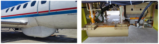
Figure 25.
Cessna 550 aircraft with ATICI.
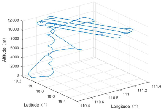
Figure 26.
Flight trajectory.
The aircraft first flies to an open sea area 250 km above land and then performs eight turnaround flights. It climbs to an altitude of 10 km during the first turnaround flight, and the observation distance for a single turnaround flight is 90 km. During the flight, the ambient load is not heated, and the warm load is heated by a heating plate. After scanning 800 times, the warm load value tends to stabilize, and the observed brightness temperature value at this time has a reference value. Excluding the process of aircraft climbing and landing, the time period during which the aircraft flies steadily in the 12 km troposphere is selected because the contribution of the atmosphere above the troposphere to the observed brightness temperature is very small, the observed brightness temperature is closer to the true brightness temperature, and the error of the radiation transfer model is also smaller.
The input data for the simulation is CMA-MESO (China Meteorological Administration Mesoscale Numerical Forecasting), and the radiation transfer model uses the RTTOV model to simulate the observed brightness temperature during computer-based flight. Considering the impact of aircraft vibration on the observation angle during airborne flight, point data below the aircraft was selected for comparison between the simulated and observed brightness temperature. Taking channel 325.15 ± 3.5 V GHz as an example, the fluctuation trend of the observed brightness temperature was basically consistent with that of the simulated brightness temperature. As shown in Figure 27 and Figure 28.
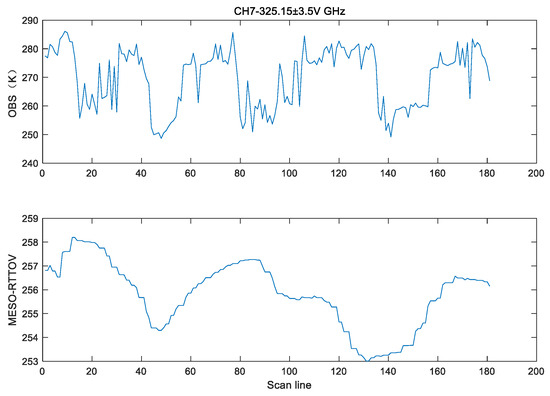
Figure 27.
Observe the fluctuation trend between brightness temperature and simulated brightness temperature.
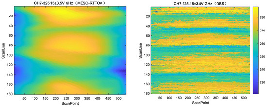
Figure 28.
Observing brightness temperature and simulating brightness temperature.
The RMSE between the airborne observation brightness temperature and the simulated brightness temperature in each channel is shown in Table 10.
Table 10.
RMSE between airborne observation brightness temperature and simulated brightness temperature in each channel.
5. Conclusions
An ICI will be launched on the next generation of the Fengyun satellite. It can detect ice water paths, ice particle size, ice water content, and cloud height, and continuously acquire upper tropospheric water vapor and ice cloud data in real-time, and this data can be applied to numerical weather prediction to improve the accuracy of weather forecasting. The ATICI was developed as an airborne demonstration aircraft for ICI and carried out a series of flight demonstrations on a Cessna 550 aircraft in 2023. It adopts a receiving front-end design scheme of a pair of plane mirrors and a quasi-optical feed network, and achieves bottom-sky observation of ice and water particles in clouds through circular scanning of a rotating antenna feed system. This design solution solves the spatial environmental adaptability problem of the feed array and the heat dissipation problem of the receiving front-end in foreign systems. Secondly, the main beam efficiency of each frequency band is improved, which in turn improves the detection accuracy of the detector. The calibration scheme achieves the scanning imaging of ice clouds and the two-point calibration of ATICI through a circular scanning and warm-ambient load calibration approach. Finally, data acquisition and processing are carried out through the data acquisition (DAQ) and control subsystem. The noise temperature of the receiver front-end is better than 4500 K, and the sensitivity analysis result of the ATICI system is better than 1.5 K. The RMSE between airborne observation brightness temperature and simulated brightness temperature is less than 26.1 K. The input data for the simulation is CMA-MESO (China Meteorological Administration Mesoscale Numerical Forecasting), and the radiation transfer model uses the RTTOV model to simulate the observed brightness temperature during computer-based flight. The comparison with the observed zenith brightness temperature over the troposphere observed by ATICI shows excellent consistency. The flight verification results show that the quasi-optical feed network subsystem works well and performs stably under vibration and temperature changes. The system sensitivity is better than 1.5 K, and the domestically produced high-frequency receiver has stable performance, which can meet the conditions of satellite applications. The ATICI performs well and meets expectations, verifying the feasibility of the Fengyun-5 ICI payload. In the future, ATICI will be used to validate the radiative-transfer model at sub-millimeter wavelengths for both clear and cloudy conditions, and to test the inversion algorithm for cloud ice properties. It can also provide calibration verification for ICI calibration.
Author Contributions
Conceptualization, R.L. and W.G.; methodology, R.L. and W.G.; software, C.W., validation, Z.H. and Y.L.; investigation, F.L., C.Z., D.S. and Y.Z.; resources, J.S. and F.D.; writing—original draft preparation, W.G.; writing—review and editing, R.L.; visualization, W.G. and C.W.; supervision, X.W. All authors have read and agreed to the published version of the manuscript.
Funding
This research was funded by the Pre-research Project of Civil Aerospace Technology of China (D010201).
Data Availability Statement
The data presented in this study are available on request from the corresponding author. The data are not publicly available due to privacy reasons.
Conflicts of Interest
The authors declare no conflicts of interest.
References
- Evans, K.F.; Stephens, G.L. Microwave radiative transfer through clouds composed of realistically shaped ice crystals. Part II: Remote sensing of ice clouds. J. Atmos. Sci. 1995, 52, 2041–2057. [Google Scholar] [CrossRef]
- Evans, K.F.; Walter, S.J.; Heymsfield, A.J.; Deeter, M.N. Modeling of submillimeter passive remote sensing of cirrus clouds. J. Appl. Meteorol. 1998, 37, 184–205. [Google Scholar] [CrossRef]
- Buehler, S.A.; Jiménez, C.; Evans, K.F.; Eriksson, P.; Rydberg, B.; Heymsfield, A.J.; Stubenrauch, C.J.; Lohmann, U.; Emde, C.; John, V.O.; et al. A concept for a satellite mission to measure cloud ice water path, ice particle size, and cloud altitude. Q. J. R. Meteorol. Soc. 2007, 133, 109–128. [Google Scholar] [CrossRef]
- Jiménez, C.; Buehler, S.A.; Rydberg, B.; Eriksson, P.; Evans, K.F. Performance simulations for a submillimetre-wave satellite instrument to measure cloud ice. Q. J. R. Meteorol. Soc. 2007, 133, 129–149. [Google Scholar] [CrossRef]
- Waliser, D.E.; Li, J.F.; Woods, C.P.; Austin, R.T.; Bacmeister, J.; Chern, J.; Del Genio, A.; Jiang, J.H.; Kuang, Z.; Meng, H.; et al. Cloud ice: A climate model challenge with signs and expectations of progress. J. Geophys. Res. Atmos. 2009, 114. [Google Scholar] [CrossRef]
- Kangas, V.; D’Addio, S.; Klein, U.; Loiselet, M.; Mason, G.; Orlhac, J.C.; Gonzalez, R.; Bergada, M.; Brandt, M.; Thomas, B. Ice cloud imager instrument for MetOp Second Generation. In Proceedings of the 2014 Specialist Meeting on Microwave Radiometry and Remote Sensing of the Environment (MicroRad), Pasadena, CA, USA, 24–27 March 2014. [Google Scholar]
- Eriksson, P.; Rydberg, B.; Mattioli, V.; Thoss, A.; Accadia, C.; Klein, U.; Buehler, S.A. Towards an operational Ice Cloud Imager (ICI) retrieval product. Atmos. Meas. Tech. 2019, 13, 53–71. [Google Scholar] [CrossRef]
- Hayton, D.J.; Ade, P.A.; Evans, K.F. Submillimeter/far-infrared channel selection simulations for a cirrus radiometer. In Proceedings of the SPIE—The International Society for Optical Engineering, Maspalomas, Canary Islands, Spain, 13–16 September 2004; Volume 5571, pp. 441–450. [Google Scholar]
- Fox, S.; Lee, C.; Moyna, B.; Philipp, M.; Rule, I.; Rogers, S.; King, R.; Oldfield, M.; Rea, S.; Henry, M.; et al. ISMAR: An airborne submillimetre radiometer. Atmos. Meas. Tech. 2017, 10, 477–490. [Google Scholar] [CrossRef]
- Fox, S.; Lee, C.; Rule, I.; King, R.; Rogers, S.; Harlow, C.; Baran, A. ISMAR: A new Submillimeter Airborne Radiometer. In Proceedings of the 2014 13th Specialist Meeting on Microwave Radiometry and Remote Sensing of the Environment (MicroRad), Pasadena, CA, USA, 24–27 March 2014; pp. 128–132. [Google Scholar]
- Brath, M.; Fox, S.; Eriksson, P.; Harlow, R.C.; Burgdorf, M.; Buehler, S.A. Retrieval of an ice water path over the ocean from ISMAR and MARSS millimeter and submillimeter brightness temperatures. Atmos. Meas. Tech. 2018, 11, 611–632. [Google Scholar] [CrossRef]
- Evans, K.F.; Wang, J.R.; Racette, P.E.; Heymsfield, G.; Li, L. Ice Cloud Retrievals and Analysis with Data from the Conical Scanning Submillimeter Imaging Radiometer and the Cloud Radar System during CRYSTAL-FACE. J. Appl. Meteor. 2005, 44, 839–859. [Google Scholar] [CrossRef]
- Li, S.; Liu, L.; Gao, T.; Huang, W.; Hu, S. Sensitivity analysis of terahertz wave passive remote sensing of cirrus microphysical parameters. Acta Phys. Sin. 2016, 65, 134102. [Google Scholar]
- Martin, R.J.; Martin, D.H. Quasi-optical antennas for radiometric remote-sensing. Electron. Commun. Eng. J. 1996, 8, 37–48. [Google Scholar] [CrossRef]
- Pan, Y.; Dong, J. Design and optimization of an ultrathin and broadband polarization-insensitive fractal FSS using the improved bacteria foraging optimization algorithm and curve fitting. Nanomaterials 2023, 13, 191. [Google Scholar] [CrossRef] [PubMed]
- Pan, Y.; Dong, J.; Wang, M. Equivalent circuit-assisted multi-objective particle swarm optimization for accelerated reverse design of multi-layer frequency selective surface. Nanomaterials 2022, 12, 3846. [Google Scholar] [CrossRef] [PubMed]
- Hu, F.; Song, Y.; Huang, Z.; Yichen, L.; Ma, X.; Wan, L. Design optimization of modular configuration for deployable truss antenna reflector. Chin. Space Sci. Technol. 2022, 42, 99–106. [Google Scholar]


Disclaimer/Publisher’s Note: The statements, opinions and data contained in all publications are solely those of the individual author(s) and contributor(s) and not of MDPI and/or the editor(s). MDPI and/or the editor(s) disclaim responsibility for any injury to people or property resulting from any ideas, methods, instructions or products referred to in the content. |
© 2024 by the authors. Licensee MDPI, Basel, Switzerland. This article is an open access article distributed under the terms and conditions of the Creative Commons Attribution (CC BY) license (https://creativecommons.org/licenses/by/4.0/).