Article

DEDNet: Dual-Encoder DeeplabV3+ Network for Rock Glacier Recognition Based on Multispectral Remote Sensing Image

1
School of Earth Science and Resources, Chang’an University, Xi’an 710054, China
2
State Key Laboratory of Tibetan Plateau Earth System, Environment and Resources (TPESER), Institute of Tibetan Plateau Research, Chinese Academy of Sciences, Beijing 100101, China
3
Shaanxi Key Laboratory of Land Consolidation, School of Land Engineering, Chang’an University, Xi’an 710054, China
4
Geological Survey of Pakistan, Peshawar 25100, Pakistan
*
Author to whom correspondence should be addressed.
These authors contributed equally to this work.
Remote Sens. 2024, 16(14), 2603; https://doi.org/10.3390/rs16142603
Submission received: 23 May 2024 / Revised: 10 July 2024 / Accepted: 14 July 2024 / Published: 16 July 2024

Abstract

:
Understanding the distribution of rock glaciers provides key information for investigating and recognizing the status and changes of the cryosphere environment. Deep learning algorithms and red–green–blue (RGB) bands from high-resolution satellite images have been extensively employed to map rock glaciers. However, the near-infrared (NIR) band offers rich spectral information and sharp edge features that could significantly contribute to semantic segmentation tasks, but it is rarely utilized in constructing rock glacier identification models due to the limitation of three input bands for classical semantic segmentation networks, like DeeplabV3+. In this study, a dual-encoder DeeplabV3+ network (DEDNet) was designed to overcome the flaws of the classical DeeplabV3+ network (CDNet) when identifying rock glaciers using multispectral remote sensing images by extracting spatial and spectral features from RGB and NIR bands, respectively. This network, trained with manually labeled rock glacier samples from the Qilian Mountains, established a model with accuracy, precision, recall, specificity, and mIoU (mean intersection over union) of 0.9131, 0.9130, 0.9270, 0.9195, and 0.8601, respectively. The well-trained model was applied to identify new rock glaciers in a test region, achieving a producer’s accuracy of 93.68% and a user’s accuracy of 94.18%. Furthermore, the model was employed in two study areas in northern Tien Shan (Kazakhstan) and Daxue Shan (Hengduan Shan, China) with high accuracy, which proved that the DEDNet offers an innovative solution to more accurately map rock glaciers on a larger scale due to its robustness across diverse geographic regions.

1. Introduction

As a predominant type of cryospheric landform [1], rock glaciers play a significant hydrological role because of their high ratio of ice content, especially in arid and semiarid areas, such as the Qilian Mountains (QLMs) [2], where water security issues cause for concern, and rock glaciers situated at higher elevations may function as freshwater reserves in the future [3]. In addition, the rock glaciers may contain paleoclimatic information [4], which is a pivotal factor in semiquantitatively assessing the meteorological environment of the forming period [5] and climate change on a local or regional scale [6]. Therefore, the recognition and delineation of rock glaciers are meaningful and helpful for evaluating their hydrological contribution [3] and studying environment change and rock glacier dynamics [7].
In addition to field measurements [8], the combination of remote sensing images and Geographic Information System technologies with manual interpretation are used for identifying rock glaciers [9], but these methods are time-consuming [10]. In recent years, studies have attempted to implement self-designed convolutional neural networks [11] along with object-based image analysis [12] to identify rock glaciers in different regions using synthetic aperture radar coherence, multispectral images, and digital elevation models, which offer valuable methods to map rock glaciers automatically. Moreover, researchers have trained some mature deep learning networks [10], especially the robust classical DeeplabV3+ network (CDNet) [13], using the RGB bands from high-resolution satellite images as training imagery [14,15], and multisource rock glacier inventories as ground truth data [16].
However, the rich spectral information and sharp edge features in the near-infrared (NIR) band [17] are helpful for rock glacier recognition because the front and lateral margins with relatively high reflectance could serve as mandatory and general geomorphological criteria for identifying rock glaciers [18,19]. Therefore, adding NIR as an additional input to RGB images can enhance the ability to distinguish between rock glaciers and surrounding landforms, as well as improve the precision of delineating rock glacier boundaries. Despite this, the NIR band has rarely been utilized in constructing semantic segmentation models for rock glaciers based on CDNet, primarily because CDNet can only accept the inputting of three image bands and is limited to processing multispectral images [15]. Therefore, most of the CDNet-based models designed for rock glacier recognition could only use the three-band natural color images as input datasets [13,14,15]. The pretrained model could be fine-tuned to obtain a localized model [20]. Thus, designing a network that simultaneously extracts and fuses spatial and spectral features from three visible bands (red–green–blue, RGB) and the NIR band is helpful for improving rock glaciers’ segmentation [21]. Additionally, there are extensive regions where rock glacier inventories are currently lacking. Employing this network will significantly aid in obtaining comprehensive information on the worldwide distribution of rock glaciers.
In semantic segmentation tasks, powerful backbones are typically employed to extract features [21]. The High-Resolution Net Version 2 (HRNetV2), as a robust backbone [22], has been extended to remote sensing image segmentation tasks [23]. The HRNetV2 exhibits strong capability in maintaining high-resolution representations through the whole process for extracting and fusing features [24], which is based on the mechanism of parallel multiresolution convolutions combined with repeated multiresolution fusions [22]. This capability of HRNetV2 effectively extracts the spatial information, boundary details, and global relationships in images, which are highly beneficial for image segmentation [25].
In this work, the main aim is to design a deep learning network capable of effectively processing images with more than three bands. Additionally, for the first time, this network will be trained using NIR bands that are more sensitive to boundary information as a data source, aiming to accurately identify rock glaciers. Therefore, a dual-encoder DeeplabV3+ network (DEDNet) with backbone of HRNetV2-W48 (also called HRNetV2 for simplicity) was designed to optimize the CDNet for processing multispectral remote sensing images and to identify rock glaciers based on GaoFen1/6 (GF1/6) satellite images.

2. Study Area and Materials

2.1. Study Area

The study area is located at the northeast of the QLMs in the northeastern edge of the Tibetan Plateau (Figure 1a,b), covering the Qilian county [38.176, 100.247] and Menyuan county [37.375, 101.611] in Qinghai province (the decimal latitude–longitude (dLL) method was used for geolocation because of its findability, accessibility, interoperability, and reusability [26]). The primary manifestation of the study area is the multiple parallel mountains, where the developed landforms continuously supply fresh water to the Heihe and Shiyang Rivers, nourishing the Hexi Corridor and surrounding areas [27]. The QLMs are characterized by extensive distribution of active, transitional, and relict type rock glaciers, particularly concentrated in the northeastern region [28]. To develop a model capable of identifying these diverse types of rock glaciers, it is imperative to compile a dataset that includes samples representing all three categories. Therefore, four subareas, referred to as visual interpretation areas (VIAs), were selected for manual interpretation of the rock glaciers (Figure 1c). Subareas A and C exhibit a prevalence of active and transitional rock glaciers, whereas transitional and relict rock glaciers dominate in subareas B and D. These areas served as the foundation for constructing a dataset for training the DEDNet. Additionally, another separate subregion, known as the model test area (MTA), was selected to assess the model’s robustness. The mountain ridges within the MTA are covered by glaciers and snow, creating favorable conditions for rock glacier development.

2.2. Imagery

Seventeen scenes of GF1/6 satellite images (http://www.sasclouds.com/chinese/home, (accessed on 5 September 2023)) were used in this study (Table 1). The GF1/6 images include four multispectral bands (RGB and NIR) with an 8 m spatial resolution and a panchromatic band with a 2 m spatial resolution. Radiometric calibration and atmospheric correction using QUAC were employed for GF1/6 images. Subsequently, image fusion based on Gram–Schmidt pan-sharpening was used to preprocess the GF1/6, through Envi5.6 software, to produce four pansharpened multispectral bands with 2 m pixels. After that, geographic registration based on Google Earth images was conducted using the ArcGIS 10.8 platform. Due to the significance of vegetation indices in rock glacier recognition [12], the SAVI (Soil Adjusted Vegetation Index) [29] and EVI (Enhanced Vegetation Index) [30] were computed using the NIR, R, and B bands of GF1/6 data. Subsequently, RGB bands were extracted to produce true color images. The NIR band, EVI, and SAVI were then combined into new three-band images, referred to as spectral images, through layer stacking.

3. Methodology

The methodology consists of five crucial steps (Figure 2). First, the rock glaciers in the VIAs and MTA were manually delineated (RG_man) based on the baseline concepts proposed by the International Permafrost Association Action Group [19], and field-investigated geomorphologic features, including physical characteristics, vegetation coverage, etc. Secondly, DEDNet is designed with two encoders and a decoder. Two encoders are used to independently extract spatial features from true color images, as well as spectral information and edge features from spectral images. The decoder is used to effectively fuse spectral and spatial information, leveraging reflectance differences to distinguish rock glaciers from surrounding landforms. Additionally, fusing edge features extracted from NIR enhances the precision of delineating rock glacier boundaries. Third, the labeled images were used to train the DEDNet to obtain a model to identify rock glaciers. Fourth, a workflow was proposed to map and post-process rock glaciers, with the well-trained model (RG_mm) based on the true color images and spectral images in VIAs and MTA. Fifth, the area of each RG_mm was calculated and compared to that of RG_man to assess the model’s accuracy in the VIAs and its robustness in the MTA.

3.1. Delineating Rock Glaciers with GF1/6 Images and Google Earth

In order to ascertain the geomorphological features of rock glaciers in the QLMs based on the baseline concepts [19], a field investigation was conducted from 1 August to 15 August 2023 (Figure 3a1–d1). The main body of rock glaciers is identifiable based on the field-investigated features such as ridges–furrows and heterogeneous vegetation distribution in natural color images, but accurately delineating the boundary is challenging (Figure 3a2–d2). With the help of a 3D oblique view on Google Earth (https://earth.google.com (accessed on 17 October 2023)), the delineation of boundaries became more accessible since the elevation difference between the edge of rock glaciers and the valley is obvious (Figure 3a3–d3). Utilizing the ArcGIS 10.8 platform for assistance, the rock glaciers were meticulously outlined and checked, resulting in 608 polygons in VIAs and 190 polygons in MTA, respectively. The polygons covered mainly by snow and clouds in the natural color images were discarded due to their serious hindering effect for the recognition of rock glaciers [11,13,14]. This is because they cover or obscure parts or all of the rock glaciers, making the geomorphological features of the rock glaciers blurred or unrecognizable. As a result, 542 snow-free and cloud-free polygons in VIAs and 190 in MTA were ultimately retained.

3.2. Designing the DEDNet

The DEDNet, based on the CDNet, inherits the classical encoder–decoder structure, where the two encoder modules extract low-level and high-level features by utilizing HRNetV2 and multiscale atrous convolution, and the decoder module refines segmentation results by fusing these features (Figure 4). Low-level features typically encompass more local details and texture information, thereby enhancing the precision of delineating rock glaciers’ boundaries. In contrast, high-level features capture global semantic information, aiding in the identification and differentiation of rock glaciers from non-rock glaciers. By fusing these two types of features, DEDNet can simultaneously preserve both details and global context, improving the understanding of spatial distribution and semantic relationships of rock glaciers in images, thus enhancing the consistency and accuracy of rock glacier identification results. Considering the training efficiency, each encoder is designed to process images with three channels, then the pretrained HRNetV2 can be used through transfer learning. The first encoder processes true color images to extract spatial features like texture, shape, and spatial relationships, while the second encoder handles spectral images to extract edge features and spectral information. Two blocks were designed and incorporated into the decoder module to fuse spatial and spectral features. Block 1 was utilized to fuse low-level features, such as local texture, shape, and edge [31], while block 2 was utilized to fuse high-level contextual information in semantic features [32]. In block 1, low-level feature 1, extracted from true color images, and low-level feature 2, extracted from spectral images (both with a shape of 256 × 88 × 88, where 256 represents the channels, and 88 represents the height and width), were initially concatenated to form a new feature map (with a shape of 512 × 88 × 88). The channels of the new feature map are twice that of each low-level feature. Then, dimensionality reduction was performed on the new feature map using 1 × 1 convolutional operations to match the dimensions of each low-level feature. Inspired by the residual network [33], a shortcut connection was embedded into block 1 to add low-level feature 1 to the new feature map. This addition maximally preserves the low-level information crucial for distinguishing interclass difference [34], as these features are primarily obtained from the true color images [35], which provide rich color information and texture details. Apart from the shortcut connection operation, block 2 mirrors the structure of block 1. Since high-level semantic information contributes to semantic image segmentation [36], only concatenation and dimensionality reduction operations were carried out in block 2.

3.3. Training and Validating the DEDNet

3.3.1. Preparing the Training and Validation Dataset

The true color images and spectral images were used to create a dataset for training the DEDNet. In this dataset, 542 snow-free and cloud-free RG_man polygons in the VIAs were employed to generate positive samples and their corresponding labels, while 1353 landforms with textures similar to rock glaciers were selected from areas near the rock glaciers to generate negative samples and their labels. To generate positive samples, we initially created 2 km × 2 km rectangles by buffering the centroid of each rock glacier polygon with a distance of 1 km. Then, the true color images and spectral images were clipped using these rectangles. For negative sample creation, we generated 1353 rectangles of 2 km × 2 km, covering the 1353 landforms, and subsequently clipped the true color images and spectral images. After that, each layer of both positive and negative samples was normalized by the maximum and minimum values for relevant layer of all the samples. Finally, as the samples with a spatial resolution of 2 m exceed the memory limit of the GPU we used when training the DEDNet, they were resampled to a 4 m pixel size to accommodate computer performance. The positive labels were generated by creating binary raster images for each positive sample, with pixel values assigned based on the presence of rock glaciers. Pixels within the rock glacier polygons, which were delineated with GF1/6 images and Google Earth based on the baseline concepts and field-investigated geomorphologic features, were assigned 1, representing the presence of rock glaciers, while pixels outside the polygons were assigned 0, representing the background. Similarly, the negative labels were generated by creating raster images with a single pixel value of 0 for each negative sample. To avoid data leakage, we picked the positive samples and labels that consist of either a single or 2 to 3 rock glaciers that were not contained in the other positive samples as the validation set. The remaining positive samples and labels were selected as the training set. Following an 8:2 ratio, the 542 positive samples were divided into 433 for training and 109 for validation, while the 1353 negative samples were split into 1082 for training and 271 for validation.

3.3.2. Training and Validating the DEDNet

The DEDNet was trained and validated with some universal hyperparameters, including optimizer—Adaptive Moment Estimation, initial learning rate—3×10⁻⁵, learning rate scheduler—cosine, base size—500 × 500 pixels, crop size—352 × 352 pixels, batch size—4, etc. The Dice loss function was selected to address data imbalance issues [37], given that rock glaciers occupy a small portion in alpine landforms [13]. The pretrained HRNetV2, downloaded from the PyTorch official website, was used for transfer learning to train the DEDNet. The DEDNet was trained on an NVIDIA GeForce RTX 4080 GPU (NVIDIA Corporation, Santa Clara, CA, USA).

3.3.3. Evaluating Metrics

Accuracy, precision, recall, specificity, and mIoU (mean intersection over union) were employed to comprehensively assess model performance. Among them, accuracy is the percentage of true rock glaciers and background in all pixels. Precision is the percentage of true rock glaciers in all detected rock glaciers. Recall is the percentage of the true rock glaciers in all manually labeled rock glaciers. Specificity is the percentage of true background in all manually labeled backgrounds. The mIoU, providing an overall assessment of segmentation accuracy, is the average of the intersection over union scores for rock glaciers and backgrounds.

3.4. Testing the Well-Trained Model

3.4.1. Preparing the Test Dataset

Testing the model robustness using the 190 RG_man polygons in MTA is insufficient to assess the overall performance of the model, such as its propensity to mistakenly identify surrounding landforms with textures similar to rock glaciers. Instead, GF1/6 images covering the MTA should be fed into the model to identify rock glaciers. Therefore, a fishing net covering MTA with each rectangle size of 1 km × 1 km was produced and then used to create the test dataset, following the steps of generating positive samples. In the test dataset, any two adjacent samples overlapped with an area of half the size of each sample, which allowed the well-trained model to identify the same rock glacier from different perspectives.

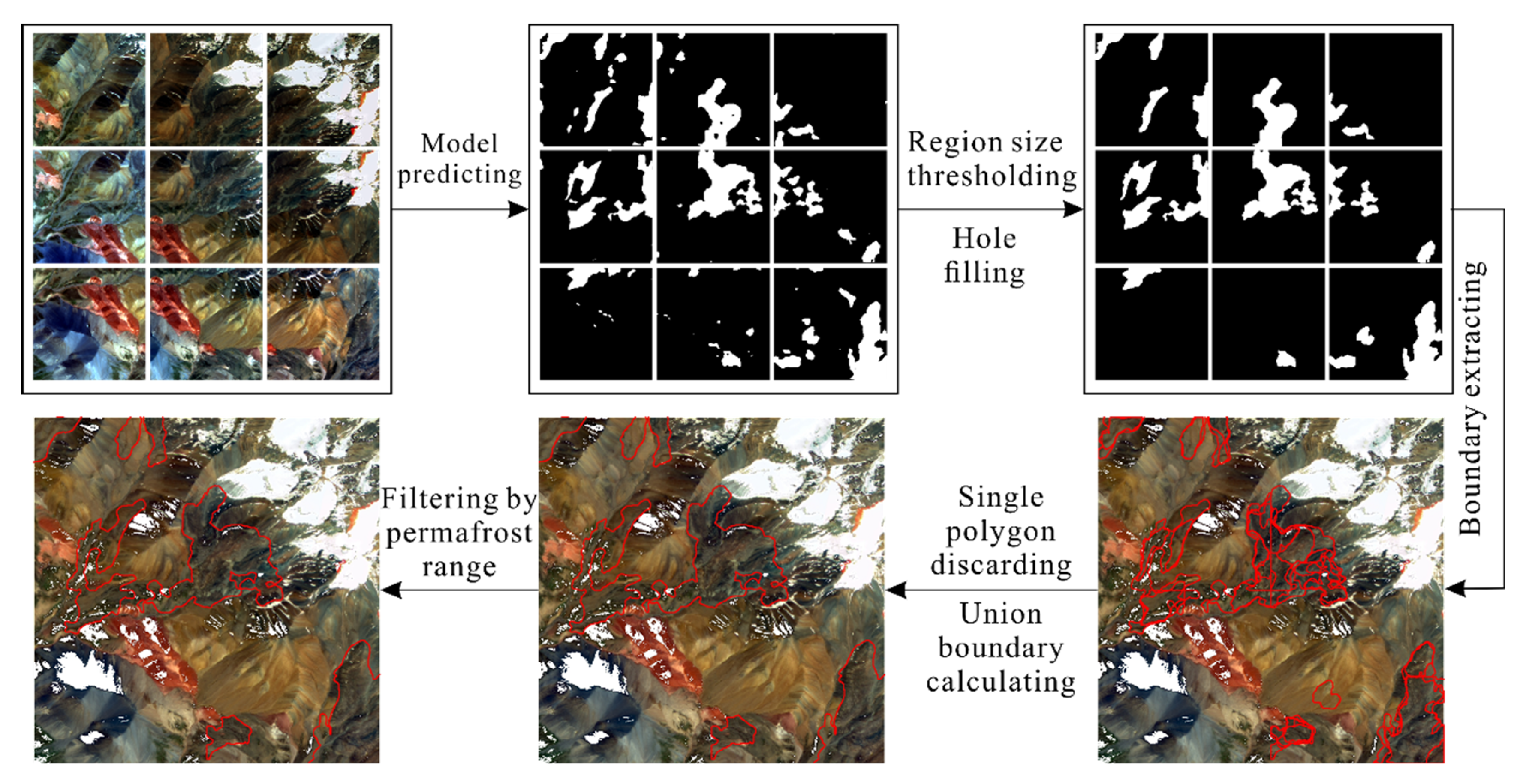
3.4.2. Mapping and Post-Processing Rock Glaciers

Several post-processing steps (Figure 5) were implemented to improve the quality of recognition results. (1) The lowest area threshold, the smallest area among all manually interpreted rock glacier polygons, was set to remove polygons smaller than 0.022 km2. (2) The holes enclosed in the RG_mm polygons were filled for continuity. (3) The RG_mm polygons were extracted from all test samples and were converted into vectors. (4) The single polygon that did not intersect with other ones was discarded, which might be misidentified due to a certain degree of randomness during the recognition process. (5) The union boundary of multiple intersection polygon vectors was calculated. (6) All polygons located within the permafrost range [38] were retained since rock glaciers are mainly distributed in the permafrost zone [9].

3.4.3. Testing Method and Metrics

The model evaluation metrics selected during the training and validating the DEDNet can assess the overall performance of the model, posing challenges for evaluating the recognition accuracy of individual rock glaciers. Therefore, following the evaluation method in [12], we employ the user’s accuracy (the percentage of the model classification that is actually a rock glacier) and the producer’s accuracy (the percentage of total rock glaciers that were classified by the model) to evaluate the model performance. In addition, to further explore the identification accuracy of individual rock glaciers, we also extracted each polygon’s area from the RG_mm and then compared that from RG_man to compute the area deviation. However, while mapping the new rock glaciers, the calculation of the union boundary of multiple intersection vectors may result in multiple adjacent rock glaciers being represented as a single one. Thus, the area-extracting method was designed with three scenarios: the first scenarios is a single RG_man polygon surrounded by a single RG_mm polygon or vice versa, where the polygon area of RG_man corresponds to that of RG_mm. We calculated the area of each rock glacier individually (Figure 6A). In the second scenario, several RG_man polygons are surrounded by a single RG_mm, where the combined area of these RG_man polygons corresponds to the area of the single RG_mm. We calculated the combined area of several RG_man polygons and the area of the single RG_mm polygon (Figure 6B). The last scenario is the opposite of the second scenario, where we calculated the combined area of several RG_mm polygons and the area of the single RG_man polygon (Figure 6C). After that, we computed the area deviation by taking the absolute value of the difference in polygon area between RG_man and RG_mm. The polygon area of RG_man and RG_mm was plotted in scatter plots, and the area deviations were used to create box plots, facilitating the analysis of recognition accuracy for individual rock glaciers.

4. Results

After 100 epochs of training and validating, the model converged with the loss value on the validation set floating around 0.20 (Figure 7), and we obtained the best model with an accuracy, precision, recall, specificity, and mIoU of 0.9131, 0.9130, 0.9270, 0.9195, and 0.8601, respectively, on the validation set. Subsequently, following the steps in the flowchart (Figure 5), the model was employed to map rock glaciers in VIAs and MTA, respectively.

4.1. Mapping Rock Glaciers in VIAs

Compared to the 542 RG_man polygons, the model identified 536 of them, and only 6 rock glaciers with an area less than 0.11 km2 were not recognized (Table S1). Additionally, the model erroneously identified 17 non-rock glaciers as rock glaciers due to their textural similarity (Table S1). The total area of 542 RG_man polygons is 155.07 km2, while the model delineated an area of 174.27 km2, indicating an overestimation of 12.38%. This is mainly because multiple adjacent rock glaciers may be represented as a single one [15], causing the inclusion of non-rock glacier areas between them.
We selected several representative polygons of RG_man and their corresponding RG_mm from four subareas to illustrate the strengths and weaknesses of the model (Figure 8). Overall, the RG_mm polygons on the validation dataset are visually accurate, and the boundaries of RG_mm are natural and basically consistent with RG_man, especially in subareas A, B, and C (Figure 8c–e), where the rock glaciers are active or transitional and exhibit readily identifiable morphological features. However, in subregion D, the rock glaciers are mainly relict, featuring indistinct morphological features and vegetation coverage similarity to surrounding landforms, resulting in insufficient consistency between the boundaries of few RG_mm and RG_man (Figure 8f). This is consistent with previous studies showing that rock glaciers with apparent ridges and furrows could be correctly identified [11], but smaller rock glaciers with subdued topography and/or evenly distributed vegetation cover were more likely to be missed [13].
To assess the identification accuracy of each individual rock glacier, the areas of each RG_mm polygon and their corresponding RG_man polygon were extracted following the method illustrated in “3.4.3 Testing method and metrics”. Nearly all points in subareas A, B, C, and D fell near the 1:1 regression line, representing a high accuracy level in identifying each rock glacier on the training and validation dataset (Figure 9a). The range (whiskers) and interquartile range (box length) of the boxplots showed a gradually decreasing trend as the scale of rock glaciers increased, indicating an improvement in the model’s recognition accuracy with the increasing size of rock glaciers (Figure 9b).

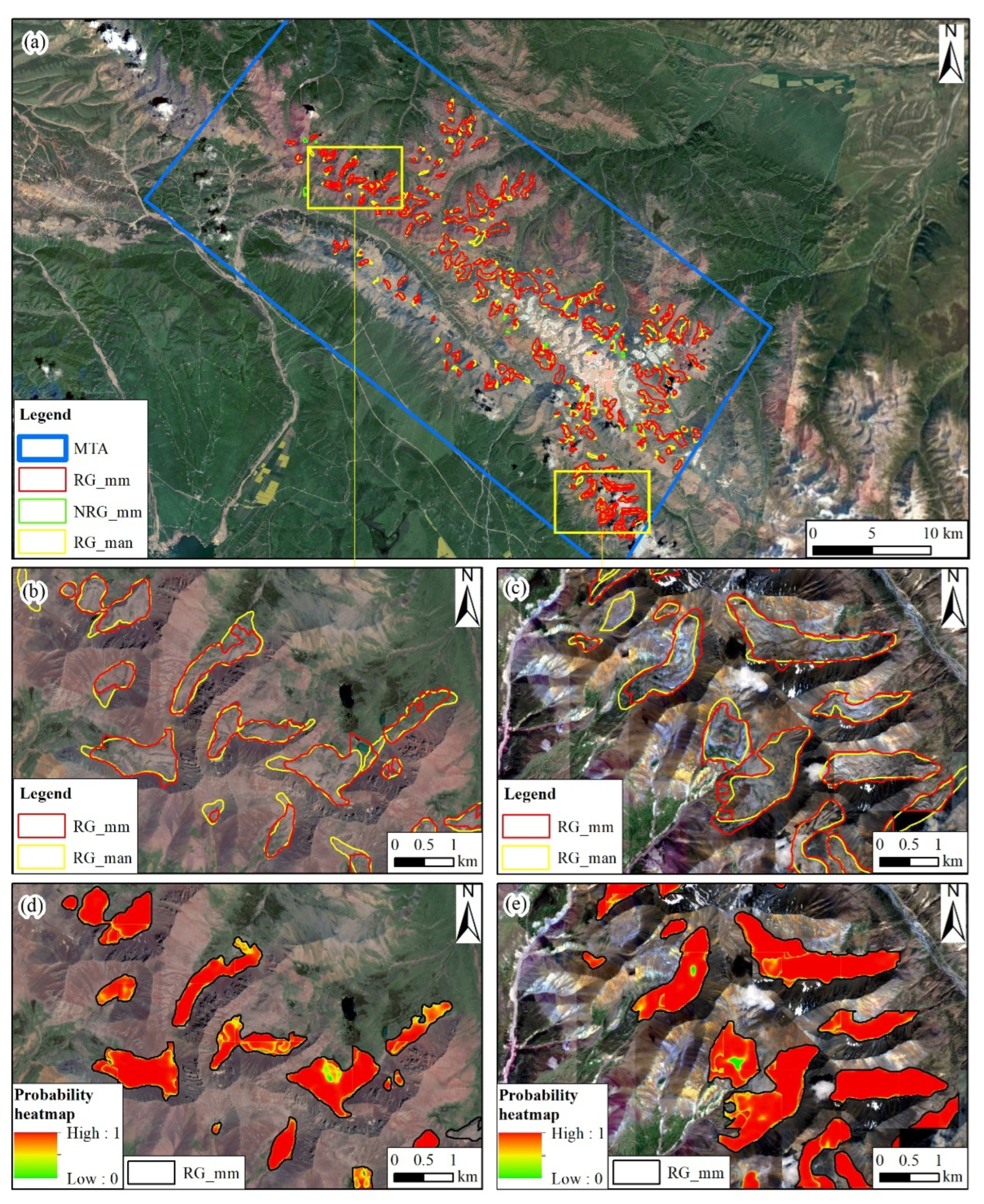
4.2. Mapping Rock Glaciers in MTA

Using the confusion matrix and metrics values (Table 2), we evaluated the model on the test dataset. The result shows that the model identified 178 out of 190 RG_man polygons with a producer’s accuracy of 93.68%. There are 12 RG_man polygons that the model failed to recognize, with the smallest area slightly larger than 0.03 km2. Additionally, the model incorrectly identified 11 non-rock glacier landforms as rock glaciers, resulting in a user’s accuracy of 94.18%. Among these 11 misclassified rock glaciers, 10 have areas smaller than 0.10 km2. Compared to larger rock glaciers, the model is more likely to misclassify rock glaciers with areas smaller than 0.10 km2.
When analyzing these 178 RG_mm polygons on the GF1/6 imagery (Figure 10a), we observed a generally high consistency between the boundaries of RG_mm and RG_man, with superior performance on larger rock glaciers compared to smaller ones (Figure 10b,c). The polygons were filled by multiple overlapping heatmaps with pixel values close to 1 (Figure 10d,e), signifying the excellent dependability of RG_mm.
Compared to the total area of 70.14 km2 of the 178 RG_man polygons, the model delineated 181 polygons with total area of 67.38 km2, indicating a slight underestimation of 3.94%. The vast majority of data points closely aligned with the 1:1 regression line, indicating a high degree of accuracy in identifying individual rock glaciers within the test area (Figure 11a). As the size of rock glaciers increased, the range (whiskers) and interquartile range (box length) of the boxplots consistently decreased, suggesting an enhancement in the model’s recognition accuracy with larger rock glaciers (Figure 11b). Estimations of individual rock glacier areas exhibit significant variation. Larger rock glaciers were generally identified and delineated with high accuracies, with an average overestimation of 1.81% for glacier areas larger than 1.00 km2, and an average underestimation of 2.51% for glacier areas between 0.50 km2 and 1.00 km2. Conversely, smaller rock glaciers exhibit lower identification accuracies, with an average underestimation of 13.57% for glacier areas between 0.1 km2 and 0.5 km2, and an average underestimation of 20.73% for glacier areas smaller than 0.10 km2.

5. Discussion

5.1. Ablation Experiment

When designing DEDNet based on the CDNet, we proposed various networks, each of which was trained on positive samples (or including negative samples) with the same hyperparameters and evaluated using mIoU, as shown in Table 3. The CDNet trained on the NIR-EVI-SAVI dataset achieved a comparable mIoU value to that trained on the RGB dataset. The model obtained by exclusively using block 2 for feature fusion in the DEDNet achieved a higher mIoU value compared to the model obtained by exclusively using block 1, indicating that high-level semantic features are more beneficial for rock glacier identification than low-level features. Of course, simultaneously applying both block 1 and block 2 to the DEDNet results in a superior rock glacier identification model, with an mIoU of 0.8519.
When training the CDNet and DEDNet including negative samples, the mIoU based on CDNet decreased from 0.8469 to 0.8457, while for the DEDNet, it increased from 0.8519 to 0.8601. The four models—training CDNet on positive samples (CDNet_Positive), training DEDNet on positive samples (DEDNet_Positive), training CDNet on positive and negative samples (CDNet_Positive_Negative), and training DEDNet on positive and negative samples (DEDNet_Positive_Negative)—were utilized to map new rock glaciers in the test area (Figure 12). The CDNet_Positive and DEDNet_Positive models classified some non-rock glacier landforms as rock glaciers, whereas the CDNet_Positive_Negative and DEDNet_Positive_Negative models significantly reduced this error, highlighting the importance of including negative samples during training [11,13]. Comparing the recognition results of models between CDNet_Positive_Negative and DEDNet_Positive_Negative, we observed that both models were able to identify larger rock glaciers (active or transitional), and they both exhibited instances where adjacent rock glaciers were delineated as a single union rock glacier (black arrows in Figure 12a1,a3), which has also been reported in other rock glacier identification models [15]. However, for delineating rock glacier boundaries, especially the smaller and relict rock glaciers, the recognition performance of DEDNet_Positive_Negative was noticeably better (white arrows in subregions of Figure 12a1,a3,b1,b3,c1,c3).
The extraction and fusion of spatial and spectral features by DEDNet enhance the accuracy of rock glacier recognition mainly because of the following: (1) For active rock glaciers, the distinct spatial features such as furrows–ridges and steep frontal and lateral margins contribute to the identification of rock glaciers. However, when combining the spatial features with spectral ones, the textural similarity landforms, such as debris-covered glaciers, could be excluded readily because the exposed ice in debris-covered glaciers could be distinguished by the lower reflectance in the NIR band. In addition, the identification accuracy of the rock glacier boundaries improved because the steep margins exhibit lighter slopes or darker shadows related to the sun position, making them easier to distinguish from the neighboring landforms due to their higher or lower spectral reflectance. (2) For transitional/relict rock glaciers, vegetation has developed along the longitudinal and transverse flow structures, as well as the frontal and lateral margins, forming distinctive and identifiable spatial features and heterogeneous vegetation spectral characteristics. This enables the differentiation of transitional/relict rock glaciers from upstream nonvegetated landforms and downstream homogeneous vegetation landforms.

5.2. Model Performance Comparison

We experimentally compare DEDNet with CDNet, modified CDNet, and the mature MSNet [21], using the training and validation datasets, which include both positive and negative samples. The CDNet is presently considered the most advanced and widely adopted method in rock glacier recognition [13,14,15,16]. There are two commonly used methods to modify CDNet for processing multispectral data: increasing the number of channels in CDNet input layer (MI_CDNet) to match the input data [39], and adding a convolution layer at the beginning of CDNet (AC_CDNet) to transform multispectral images to 3D features [40]. Furthermore, the MI_CDNet was trained without the pretrained HRNetV2 because of the structural mismatch between MI_CDNet and the pretrained HRNetV2. The significant advantages of MSNet over RTFNet [41], MUFNet [42], and MFNet [43] in processing 4-band images have been verified [21], and the comparison between MSNet and DEDNet can reflect the superiority of DEDNet to fuse spatial and spectral features in the semantic segmentation field. In addition, several powerful backbones, such as ResNet50, ResNet101, deep residual network (DRN), Xception, and Vision Transformer (VIT), were employed to replace the HRNetV2 for training the DEDNet with same hyperparameters, with the results presented in Table 4.
By training the DEDNet (with backbone of HRNetV2), we obtained the best-performing model, which outperformed the CDNet-based model and other comparative models in all evaluation metrics. The models trained with the MI_CDNet and AC_CDNet network achieved low accuracy, with mIoU values of 0.6944 and 0.7112, respectively, representing a 15 percent point decrease compared to the mIoU obtained with the DEDNet model, indicating the challenges of using CDNet for rock glacier identification on multispectral images. Comparing the models trained with MSNet and DEDNet (both using ResNet50 as the backbone) network, we found that the latter achieved an mIoU of 0.8455, slightly higher than the former’s 0.8413. This suggests that in the rock glacier identification field, the simple yet effective DEDNet is advantageous. Compared to other backbones, HRNetV2’s advantages are more pronounced, possibly because HRNetV2 maintains high-resolution representations through the whole process, aiding in distinguishing rock glaciers with spectral similarities from surrounding landforms.

5.3. Transferability of the Model

The well-trained DEDNet model was also applied to two areas with rock glacier inventories published, the northern Tien Shan (Kazakhstan) and Daxue Shan (approximately 1500 km in the south of the QLMs), to test the generalizability of the model. The northern Tien Shan, located 2500 km in the northwest of the QLMs (Figure 13a), has a rock glacier inventory including only active rock glaciers produced using InSAR kinematics [44]. A region ranging from 76°58′E to 77°13′E and 42°59′N to 43°10′N, with 54 rock glaciers according to the inventory, was selected for the generalizability research. In total, 50 out of the 54 rock glaciers (Figure 13b) were identified by the well-trained DEDNet model, with a total area of 42.63 km2, demonstrating an overestimation compared to the 32.33 km2 estimated by the InSAR kinematics, which only extracts the active “unit” of the rock glacier “system”.
The Daxue Shan [45] is located to the south of the QLMs (Figure 13d), at the southeastern edge of the Tibetan Plateau’s Hengduan Shan. A rock glacier inventory based on the analysis of Google Earth imagery has been released there. The region, ranging from 101°34′E to 101°40′E and 30°24′N to 30°32′N, contains 38 rock glaciers with different scale. The DEDNet model identified 35 out of the 38 rock glaciers (Figure 13e), with a total area of 8.58 km2, demonstrating 4.57% underestimation compared to the 8.99 km2 of the 38 rock glaciers. Rock glaciers with distinct/vague and identifiable frontal slope and furrows–ridges not in the inventories were also delineated by the DEDNet model (Figure 13c,f). Overall, our DEDNet-based model exhibits strong robustness and demonstrates great potential for applicability across diverse geographic regions.

5.4. Contribution and Limitation

When delineating rock glaciers on a large scale, DEDNet may have two foreseeable potential contributions. Firstly, The DEDNet showed its robustness when applying the DEDNet-based model to Daxue Shan and Tien Shan, demonstrating the potential capability to map rock glaciers across diverse geographic regions. Therefore, DEDNet can be employed in some alpine regions where inventories remain incomplete, to identify and delineate rock glaciers. Secondly, the model trained using DEDNet on RGB and NIR-EVI-SAVI datasets outperformed those trained solely on RGB or NIR-EVI-SAVI datasets using CDNet, even when supplemented with InSAR images [13], in identifying relict rock glaciers (Table 3). Exploring the distribution of relict rock glaciers contributes to a comprehensive understanding of the mountainous environment because of the cruciality for reconstructing ancient climates [18] and the significance for hydrogeology research [46].
DEDNet shows promise but still has two limitations. Firstly, the pretrained HRNetV2 is suitable for processing RGB datasets but is not optimized for NIR-EVI-SAVI datasets [21], which affects the extraction of spectral information. This may well explain the phenomenon: compared to the model trained using CDNet on 542 positive samples with mIoU of 0.8469, the model trained using DEDNet on the same dataset only achieved a slight increase to 0.8519, an improvement of just 0.005%. Furthermore, with the addition of 1353 negative samples, the mIoU increased from 0.8457 to 0.8601, showing a significant improvement of 0.0144%. This is because more training samples result in better fine-tuning of the pretrained model parameters. Secondly, the number of parameters of the DEDNet is approximately twice that of the CDNet. When training a rock glacier (or other landform) identification model using DEDNet, more computational resources are required. This is the reason why we resampled GF1/6 with a spatial resolution of 2 m to 4 m during the dataset preparation stage.

6. Conclusions

In this study, we designed a DEDNet with two encoders to simultaneously extract and fuse spatial and spectral features from the RGB dataset and the NIR-EVI-SAVI dataset, respectively. We trained the DEDNet with positive and negative samples including active, transitional, and relict type rock glaciers from VIAs in the QLMs and obtained a model with accuracy, precision, recall, specificity, and mIoU of 0.9131, 0.9130, 0.9270, 0.9195, and 0.8601, respectively. Then, we tested the model’s robustness in MTA and successfully identified 178 out of 190 RG_man, missing 12 small rock glaciers, and misidentifying 11 other landforms with textural similarity as rock glaciers. Ultimately, we achieved a producer’s accuracy of 93.68% and a user’s accuracy of 94.18%. Furthermore, our DEDNet demonstrates its robustness to map rock glaciers with greater accuracy across diverse geographic regions.

Supplementary Materials

The following supporting information can be downloaded at: https://www.mdpi.com/article/10.3390/rs16142603/s1. Table S1: The centroids (decimal latitude-longitude (dLL)) and images of 6 false negative and 17 false positive rock glaciers in VIAs (visual interpretation areas).

Author Contributions

Conceptualization, L.L. (Lei Liu), M.F., M.L., Y.S.K. and F.Y.; investigation, L.L. (Lujun Lin) and Q.Z.; data curation, L.L. (Lujun Lin); funding acquisition, L.L. (Lei Liu), F.Y. and L.L. (Lujun Lin); methodology, L.L. (Lujun Lin), M.L. and Q.Z.; supervision, M.L., L.L. (Lei Liu), M.F., Y.S.K. and F.Y.; project administration, L.L. (Lei Liu) and M.F.; software, L.L. (Lujun Lin); writing—original draft, L.L. (Lujun Lin) and Q.Z.; writing—review and editing, M.L., L.L. (Lei Liu) and M.F. All authors have read and agreed to the published version of the manuscript.

Funding

This work was funded by the Open Research Fund of TPESER, grant number TPESER202208; the Central University Basic Scientific Research Business Expenses Special Funds—Chang’an University Excellent Doctoral Dissertation Cultivation Support Project, grant number 300102273720; and the Natural Science Basic Research Program of Shaanxi Province, grant number 2024SF-YBXM-570.

Data Availability Statement

Data used and analyzed in the present study will be made available upon request.

Acknowledgments

The authors appreciate Google for the free use of the Google Earth Pro software (version: 7.3.6.9796). The authors also highly acknowledge Zhengchao Ren, Jinhao Xu, and Dezhao Yan for their contributions to the rock glacier field investigation in the Qilian Mountains. The permafrost distribution map made by Lin Zhao is available at https://data.tpdc.ac.cn/zh-hans/data/0231c972-8460-4691-a187-70e4cc356f60/ (accessed on 18 December 2023).

Conflicts of Interest

The authors declare no conflicts of interest.

References

  1. Azócar, G.F.; Brenning, A. Hydrological and Geomorphological Significance of Rock Glaciers in the Dry Andes, Chile (27°–33°S): Rock Glaciers in the Dry Andes. Permafr. Periglac. Process. 2010, 21, 42–53. [Google Scholar] [CrossRef]
  2. Yan, M.; Tian, X.; Li, Z.; Chen, E.; Li, C.; Fan, W. A Long-Term Simulation of Forest Carbon Fluxes over the Qilian Mountains. Int. J. Appl. Earth Obs. Geoinf. 2016, 52, 515–526. [Google Scholar] [CrossRef]
  3. Jones, D.B.; Harrison, S.; Anderson, K.; Whalley, W.B. Rock Glaciers and Mountain Hydrology: A Review. Earth-Sci. Rev. 2019, 193, 66–90. [Google Scholar] [CrossRef]
  4. Humlum, O. The Climatic Significance of Rock Glaciers. Permafr. Periglac. Process. 1998, 9, 375–395. [Google Scholar] [CrossRef]
  5. Humlum, O. Rock Glacier Appearance Level and Rock Glacier Initiation Line Altitude: A Methodological Approach to the Study of Rock Glaciers. Arct. Alp. Res. 1988, 20, 160–178. [Google Scholar] [CrossRef]
  6. Konrad, S.K.; Humphrey, N.F.; Steig, E.J.; Clark, D.H.; Potter, N.; Pfeffer, W.T. Rock Glacier Dynamics and Paleoclimatic Implications. Geology 1999, 27, 1131. [Google Scholar] [CrossRef]
  7. Harris, C.; Arenson, L.U.; Christiansen, H.H.; Etzelmüller, B.; Frauenfelder, R.; Gruber, S.; Haeberli, W.; Hauck, C.; Hölzle, M.; Humlum, O.; et al. Permafrost and Climate in Europe: Monitoring and Modelling Thermal, Geomorphological and Geotechnical Responses. Earth-Sci. Rev. 2009, 92, 117–171. [Google Scholar] [CrossRef]
  8. Petersen, E.I.; Levy, J.S.; Holt, J.W.; Stuurman, C.M. New Insights into Ice Accumulation at Galena Creek Rock Glacier from Radar Imaging of Its Internal Structure. J. Glaciol. 2020, 66, 1–10. [Google Scholar] [CrossRef]
  9. Bolch, T.; Gorbunov, A.P. Characteristics and Origin of Rock Glaciers in Northern Tien Shan (Kazakhstan/Kyrgyzstan). Permafr. Periglac. Process. 2014, 25, 320–332. [Google Scholar] [CrossRef]
  10. Feng, M.; Xu, J.; Wang, J.; Ran, Y.; Li, X. Identifying Rock Glacier in Western China Using Deep Learning and Satellite Data. In Proceedings of the AGU Fall Meeting Abstracts, San Francisco, CA, USA, 9–13 December 2019; Volume 2019, p. GC53G-1249. [Google Scholar]
  11. Marcer, M. Rock Glaciers Automatic Mapping Using Optical Imagery and Convolutional Neural Networks. Permafr. Periglac. Process. 2020, 31, 561–566. [Google Scholar] [CrossRef]
  12. Robson, B.A.; Bolch, T.; MacDonell, S.; Hölbling, D.; Rastner, P.; Schaffer, N. Automated Detection of Rock Glaciers Using Deep Learning and Object-Based Image Analysis. Remote Sens. Environ. 2020, 250, 112033. [Google Scholar] [CrossRef]
  13. Hu, Y.; Liu, L.; Huang, L.; Zhao, L.; Wu, T.; Wang, X.; Cai, J. Mapping and Characterizing Rock Glaciers in the Arid West Kunlun of China. Authorea Prepr. 2023. [Google Scholar] [CrossRef]
  14. Sun, Z.; Hu, Y.; Liu, L.; Racoviteanu, A.; Harrison, S. Mapping Rock Glaciers on the Tibetan Plateau from Planet Basemaps Using Deep Learning. In Proceedings of the AGU Fall Meeting Abstracts, Chicago, IL, USA, 12–16 December 2022; Volume 2022, p. C42E-1078. [Google Scholar]
  15. Sun, Z.; Hu, Y.; Racoviteanu, A.; Liu, L.; Harrison, S.; Wang, X.; Cai, J.; Guo, X.; He, Y.; Yuan, H. TPRoGI: A Comprehensive Rock Glacier Inventory for the Tibetan Plateau Using Deep Learning. Earth Syst. Sci. Data Discuss. 2024, 2024, 1–32. [Google Scholar]
  16. Sun, Z.; Hu, Y.; Liu, L.; Racoviteanu, A.; Harrison, S. Mapping and Inventorying Rock Glaciers on the Tibetan Plateau from Planet Basemaps Using Deep Learning. In Proceedings of the EGU General Assembly Conference Abstracts, Vienna, Austria, 23–28 April 2023; p. EGU-6816. [Google Scholar]
  17. Jiang, J.; Feng, X.; Liu, F.; Xu, Y.; Huang, H. Multi-Spectral RGB-NIR Image Classification Using Double-Channel CNN. IEEE Access 2019, 7, 20607–20613. [Google Scholar] [CrossRef]
  18. Barsch, D. Permafrost Creep and Rockglaciers. Permafr. Periglac. Process. 1992, 3, 175–188. [Google Scholar] [CrossRef]
  19. IPA Action Group Rock Glacier Inventories and Kinematics towards Standard Guidelines for Inventorying Rock Glaciers: Baseline Concepts (Version 4.2.2). 2022. 13p. Available online: https://bigweb.unifr.ch/Science/Geosciences/Geomorphology/Pub/Website/IPA/Guidelines/V4/220331_Baseline_Concepts_Inventorying_Rock_Glaciers_V4.2.2.pdf (accessed on 8 September 2023).
  20. Pan, B.; Shi, Z.; Xu, X.; Shi, T.; Zhang, N.; Zhu, X. CoinNet: Copy Initialization Network for Multispectral Imagery Semantic Segmentation. IEEE Geosci. Remote Sens. Lett. 2019, 16, 816–820. [Google Scholar] [CrossRef]
  21. Tao, C.; Meng, Y.; Li, J.; Yang, B.; Hu, F.; Li, Y.; Cui, C.; Zhang, W. MSNet: Multispectral Semantic Segmentation Network for Remote Sensing Images. GIScience Remote Sens. 2022, 59, 1177–1198. [Google Scholar] [CrossRef]
  22. Wang, J.; Sun, K.; Cheng, T.; Jiang, B.; Deng, C.; Zhao, Y.; Liu, D.; Mu, Y.; Tan, M.; Wang, X.; et al. Deep High-Resolution Representation Learning for Visual Recognition. IEEE Trans. Pattern Anal. Mach. Intell. 2021, 43, 3349–3364. [Google Scholar] [CrossRef]
  23. Yang, X.; Fan, X.; Peng, M.; Guan, Q.; Tang, L. Semantic Segmentation for Remote Sensing Images Based on an AD-HRNet Model. Int. J. Digit. Earth 2022, 15, 2376–2399. [Google Scholar] [CrossRef]
  24. Wu, H.; Liang, C.; Liu, M.; Wen, Z. Optimized HRNet for Image Semantic Segmentation. Expert Syst. Appl. 2021, 174, 114532. [Google Scholar] [CrossRef]
  25. Xu, Z.; Zhang, W.; Zhang, T.; Li, J. HRCNet: High-Resolution Context Extraction Network for Semantic Segmentation of Remote Sensing Images. Remote Sens. 2020, 13, 71. [Google Scholar] [CrossRef]
  26. Whalley, W.B. Enhancing the Digital Earth via Digital Decimal Geolocation and the FAIR Data Principles. Earth Sci. Syst. Soc. 2024, 4, 10110. [Google Scholar] [CrossRef]
  27. Lou, P.; Wu, T.; Chen, J.; Fu, B.; Zhu, X.; Chen, J.; Wu, X.; Yang, S.; Li, R.; Lin, X.; et al. Recognition of Thaw Slumps Based on Machine Learning and UAVs: A Case Study in the Qilian Mountains, Northeastern Qinghai-Tibet Plateau. Int. J. Appl. Earth Obs. Geoinf. 2023, 116, 103163. [Google Scholar] [CrossRef]
  28. Hu, Z.; Yan, D.; Feng, M.; Xu, J.; Liang, S.; Sheng, Y. Enhancing Mountainous Permafrost Mapping by Leveraging a Rock Glacier Inventory in Northeastern Tibetan Plateau. Int. J. Digit. Earth 2024, 17, 2304077. [Google Scholar] [CrossRef]
  29. Gilabert, M.A.; González-Piqueras, J.; García-Haro, F.J.; Meliá, J. A Generalized Soil-Adjusted Vegetation Index. Remote Sens. Environ. 2002, 82, 303–310. [Google Scholar] [CrossRef]
  30. Jiang, Z.; Huete, A.; Didan, K.; Miura, T. Development of a Two-Band Enhanced Vegetation Index without a Blue Band. Remote Sens. Environ. 2008, 112, 3833–3845. [Google Scholar] [CrossRef]
  31. Zhu, L.; Ji, D.; Zhu, S.; Gan, W.; Wu, W.; Yan, J. Learning Statistical Texture for Semantic Segmentation. In Proceedings of the IEEE/CVF Conference on Computer Vision and Pattern Recognition, Seattle, WA, USA, 13–19 June 2020; pp. 12975–12984. [Google Scholar]
  32. Long, J.; Shelhamer, E.; Darrell, T. Fully Convolutional Networks for Semantic Segmentation. In Proceedings of the IEEE Conference on Computer Vision and Pattern Recognition (CVPR), Boston, MA, USA, 7–12 June 2015; pp. 3431–3440. [Google Scholar]
  33. He, K.; Zhang, X.; Ren, S.; Sun, J. Deep Residual Learning for Image Recognition. In Proceedings of the 2016 IEEE Conference on Computer Vision and Pattern Recognition (CVPR), Las Vegas, NV, USA, 27–30 June 2016; pp. 770–778. [Google Scholar]
  34. Su, R.; Xu, D.; Sheng, L.; Ouyang, W. PCG-TAL: Progressive Cross-Granularity Cooperation for Temporal Action Localization. IEEE Trans. Image Process. 2021, 30, 2103–2113. [Google Scholar] [CrossRef]
  35. Yan, J.; Liu, J.; Liang, D.; Wang, Y.; Li, J.; Wang, L. Semantic Segmentation of Land Cover in Urban Areas by Fusing Multisource Satellite Image Time Series. IEEE Trans. Geosci. Remote Sens. 2023, 61, 4410315. [Google Scholar] [CrossRef]
  36. Chen, L.-C.; Papandreou, G.; Kokkinos, I.; Murphy, K.; Yuille, A.L. DeepLab: Semantic Image Segmentation with Deep Convolutional Nets, Atrous Convolution, and Fully Connected CRFs. IEEE Trans. Pattern Anal. Mach. Intell. 2018, 40, 834–848. [Google Scholar] [CrossRef]
  37. Zhao, R.; Qian, B.; Zhang, X.; Li, Y.; Wei, R.; Liu, Y.; Pan, Y. Rethinking Dice Loss for Medical Image Segmentation. In Proceedings of the 2020 IEEE International Conference on Data Mining (ICDM), Sorrento, Italy, 17–20 November 2020; pp. 851–860. [Google Scholar]
  38. Li, J.; Wang, Q.; Zhang, Y.; Yang, S.; Gao, G. An Improved Active Layer Thickness Retrieval Method over Qinghai-Tibet Permafrost Using InSAR Technology: With Emphasis on Two-Dimensional Deformation and Unfrozen Water. Int. J. Appl. Earth Obs. Geoinf. 2023, 124, 103530. [Google Scholar] [CrossRef]
  39. Carvalho, O.L.F.D.; De Carvalho Júnior, O.A.; Albuquerque, A.O.D.; Bem, P.P.D.; Silva, C.R.; Ferreira, P.H.G.; Moura, R.D.S.D.; Gomes, R.A.T.; Guimarães, R.F.; Borges, D.L. Instance Segmentation for Large, Multi-Channel Remote Sensing Imagery Using Mask-RCNN and a Mosaicking Approach. Remote Sens. 2020, 13, 39. [Google Scholar] [CrossRef]
  40. Han, W.; Li, J.; Wang, S.; Zhang, X.; Dong, Y.; Fan, R.; Zhang, X.; Wang, L. Geological Remote Sensing Interpretation Using Deep Learning Feature and an Adaptive Multisource Data Fusion Network. IEEE Trans. Geosci. Remote Sens. 2022, 60, 4510314. [Google Scholar] [CrossRef]
  41. Sun, Y.; Zuo, W.; Liu, M. RTFNet: RGB-Thermal Fusion Network for Semantic Segmentation of Urban Scenes. IEEE Robot. Autom. Lett. 2019, 4, 2576–2583. [Google Scholar] [CrossRef]
  42. Xu, F.; Shang, Z.; Wu, Q.; Zhang, X.; Lin, Z.; Shao, S. MUFNet: Toward Semantic Segmentation of Multi-Spectral Remote Sensing Images. In Proceedings of the 2021 4th Artificial Intelligence and Cloud Computing Conference, Kyoto Japan, 17–19 December 2021; pp. 39–46. [Google Scholar]
  43. Ha, Q.; Watanabe, K.; Karasawa, T.; Ushiku, Y.; Harada, T. MFNet: Towards Real-Time Semantic Segmentation for Autonomous Vehicles with Multi-Spectral Scenes. In Proceedings of the 2017 IEEE/RSJ International Conference on Intelligent Robots and Systems (IROS), Vancouver, BC, Canada, 24–28 September 2017; pp. 5108–5115. [Google Scholar]
  44. Bertone, A.; Barboux, C.; Bodin, X.; Bolch, T.; Brardinoni, F.; Caduff, R.; Christiansen, H.H.; Darrow, M.M.; Delaloye, R.; Etzelmüller, B.; et al. Incorporating InSAR Kinematics into Rock Glacier Inventories: Insights from 11 Regions Worldwide. Cryosphere 2022, 16, 2769–2792. [Google Scholar] [CrossRef]
  45. Ran, Z.; Liu, G. Rock Glaciers in Daxue Shan, South-Eastern Tibetan Plateau: An Inventory, Their Distribution, and Their Environmental Controls. Cryosphere 2018, 12, 2327–2340. [Google Scholar] [CrossRef]
  46. Colucci, R.R.; Forte, E.; Žebre, M.; Maset, E.; Zanettini, C.; Guglielmin, M. Is That a Relict Rock Glacier? Geomorphology 2019, 330, 177–189. [Google Scholar] [CrossRef]
Figure 1. (a) Location of the QLMs. (b) The location of the study area in the QLMs. (c) Location of VIAs (visual interpretation areas), MTA (model test area), field investigation, model training, model validation, and model test rock glaciers in the study area. In VIAs, the centroids of subareas A, B, C, and D are [38.314, 100.424], [38.116, 100.088], [37.526, 101.723], and [37.367, 101.315], respectively. The centroid of MTA is [37.758, 101.400].
Remotesensing 16 02603 g001
Figure 2. Flowchart of the methodology. RG_mm and RG_man represent the rock glacier model mapped and rock glacier manually delineated, respectively.
Remotesensing 16 02603 g002
Figure 3. The characteristics of four rock glaciers: (a1d1) field photos, (a2d2) GF1/6 images, and (a3d3) Google Earth 3D oblique view. The dLL locations in the first row images represent the centroid of four rock glaciers. The red lines represent the boundary of rock glaciers.
Remotesensing 16 02603 g003
Figure 4. The DEDNet with the backbone of HRNetV2 and the block 1 and block 2 we designed.
Remotesensing 16 02603 g004
Figure 5. The flowchart of mapping rock glaciers in MTA.
Remotesensing 16 02603 g005
Figure 6. Three area-extracting methods, where the area of (A) corresponds to that of a; the area of (B) corresponds to the combined area of b1, b2, b3, b4, b5, and b6; the area of (C) corresponds to the combined area of c1, c2, and c3. The centroids of polygon (AC) are [38.345, 100.334], [38.337, 100.327], and [38.355, 100.326], respectively.
Remotesensing 16 02603 g006
Figure 7. The evaluation metrics on validation set during training and validating the DEDNet.
Remotesensing 16 02603 g007
Figure 8. Comparison of boundaries between RG_mm and RG_man in VIAs (a,b). The panels (cf) correspond to the yellow box in subareas A, B, C, and D. The background images of (a,b) are the true color image composed of a combination of RGB bands of GF1/6. The background images of (cf) are a combination of NIR-G-B bands of GF1/6.
Remotesensing 16 02603 g008
Figure 9. Scatterplots illustrating the areas of RG_mm polygons compared to RG_man polygons on the training and validation datasets (a), and boxplots displaying the deviations in area across various scales on the training and validation datasets (b). In boxplots, “small” denotes areas less than 0.10 km2, “medium_s” refers to areas between 0.10 and 0.50 km2, “medium_l” signifies areas between 0.50 and 1.00 km2, and “large” indicates areas larger than 1.00 km2.
Remotesensing 16 02603 g009
Figure 10. Comparison of RG_man’s boundaries with RG_mm’s boundaries in MTA (a), along with two typical subregions (b,c), and their corresponding probability heatmap (d,e) on GF1/6 imagery. NRG_mm represents non-rock glacier model mapped. Background image is a true color image composed of a combination of RGB bands of GF1/6.
Remotesensing 16 02603 g010
Figure 11. Scatterplots illustrating the areas of RG_mm compared to RG_man on the test datasets (a), and boxplots displaying the deviations in area across various scales on the test datasets (b). Here, “small”, “medium_s”, “medium_l”, and “large” correspond to the same meanings as the terms used in Figure 9.
Remotesensing 16 02603 g011
Figure 12. Boundaries of RG_man and four models outlined in three subregions in MTA. (ac) represent three distinct subregions. 1, 2, 3, and 4 represent four different models. The four RG_models represent the rock glaciers delineated by corresponding models. For example, RG_CDNet_Positive represents rock glaciers delineated by CDNet_Positive. Black arrows represent adjacent rock glaciers mapped by one model, which were delineated as a single union rock glacier by another model. White arrows indicate that DEDNet_Positive_Negative identifies these rock glaciers better than CDNet_Positive_Negative.
Remotesensing 16 02603 g012
Figure 13. Locations of northern Tien Shan (Kazakhstan) (a) and Daxue Shan (d). Boundaries of RG_man and RG_inventory in northern Tien Shan (b) and Daxue Shan (e). Rock glaciers were model mapped but not included in the inventory of northern Tien Shan (c) and Daxue Shan (f). The background images of (b,e) are the true color image composed of a combination of RGB bands of GF1/6. The background images of (c,f) are a combination of NIR-G-B bands of GF1/6.
Remotesensing 16 02603 g013
Table 1. List of GF1/6 satellite images.
DateSensorSensor IDResolution
26 August 2015GF1GF1_PMS1_E101.4_N37.5_20150826_L1A00009998102/8 m
26 August 2015GF1GF1_PMS2_E101.8_N37.4_20150826_L1A0000999891
26 August 2015GF1GF1_PMS2_E101.8_N37.7_20150826_L1A0000999890
26 August 2015GF1GF1_PMS1_E101.5_N37.8_20150826_L1A0000999809
28 August 2020GF1GF1_PMS2_E100.4_N38.2_20200828_L1A0005019914
28 August 2020GF1GF1_PMS1_E100.0_N38.3_20200828_L1A0005019873
26 July 2020GF1GF1_PMS2_E101.4_N37.7_20200726_L1A0004951368
28 August 2020GF1GF1_PMS1_E99.9_N38.0_20200828_L1A0005019874
28 August 2020GF1GF1_PMS2_E100.3_N38.0_20200828_L1A0005019915
26 July 2020GF1GF1_PMS2_E101.4_N37.4_20200726_L1A0004951369
29 July 2020GF1GF1_PMS1_E101.0_N37.5_20200726_L1A0004951209
7 September 2021GF6GF6_PMS_E100.9_N37.3_20210907_L1A1120139417
26 August 2020GF6GF6_PMS_E100.0_N38.7_20200826_L1A1120029769
3 May 2020GF6GF6_PMS_E101.0_N38.0_20200503_L1A1119993834
1 June 2021GF6GF6_PMS_E99.3_N38.0_20210601_L1A1120110250
1 August 2021GF6GF6_PMS_E101.5_N37.3_20210801_L1A1120127842
26 August 2020GF6GF6_PMS_E99.8_N38.0_20200826_L1A1120030072
Table 2. Confusion matrix of the model on test dataset and accuracy metrics.
MetricsNoteResult
True positive (TP)Number of correct RG_mm178
False positive (FP)Number of wrong RG_mm11
False negative (FN)Number of missed RG_man12
Producer’s accuracyTP/(TP + FN)0.9368
User’s accuracyTP/(TP + FP)0.9418
Table 3. The mIoU of different networks trained with different datasets.
NetworkRGBNIR-EVI-SAVIBlock 1Block 2Negative SamplemIoU
CDNet 0.8469
CDNet 0.8464
DEDNet 0.8348
DEDNet 0.8509
DEDNet 0.8519
CDNet 0.8457
DEDNet0.8601
Table 4. The evaluation metrics of different networks on validation datasets.
NetworkBackbonePretrainedAccuracymIOUPrecisionRecallSpecificity
DEDNetHRNet V2True0.91310.86010.91300.92700.9195
CDNetHRNet V2True0.90470.84570.90450.91550.9095
MI_CDNetHRNet V2False0.78740.69440.78750.79000.7885
AC_CDNetHRNet V2True0.80730.71120.80750.80200.8045
MSNetResNet 50True0.90220.84130.90250.91250.9070
DEDNetResNet 50True0.90560.84550.90550.91450.9095
DEDNetResNet 101True0.90730.84900.90700.91750.9112
DEDNetDRNTrue0.90620.84900.90600.91900.9120
DEDNetXceptionTrue0.75630.60610.75600.66600.6990
DEDNetVITTrue0.83930.64050.83900.69000.7395
Note: the best model performance is shown in bold.
Disclaimer/Publisher’s Note: The statements, opinions and data contained in all publications are solely those of the individual author(s) and contributor(s) and not of MDPI and/or the editor(s). MDPI and/or the editor(s) disclaim responsibility for any injury to people or property resulting from any ideas, methods, instructions or products referred to in the content.

