
Evolution of Coastal Environments under Inundation Scenarios Using an Oceanographic Model and Remote Sensing Data

 ,
,  , ,
, ,  ,
,
Abstract
:1. Introduction
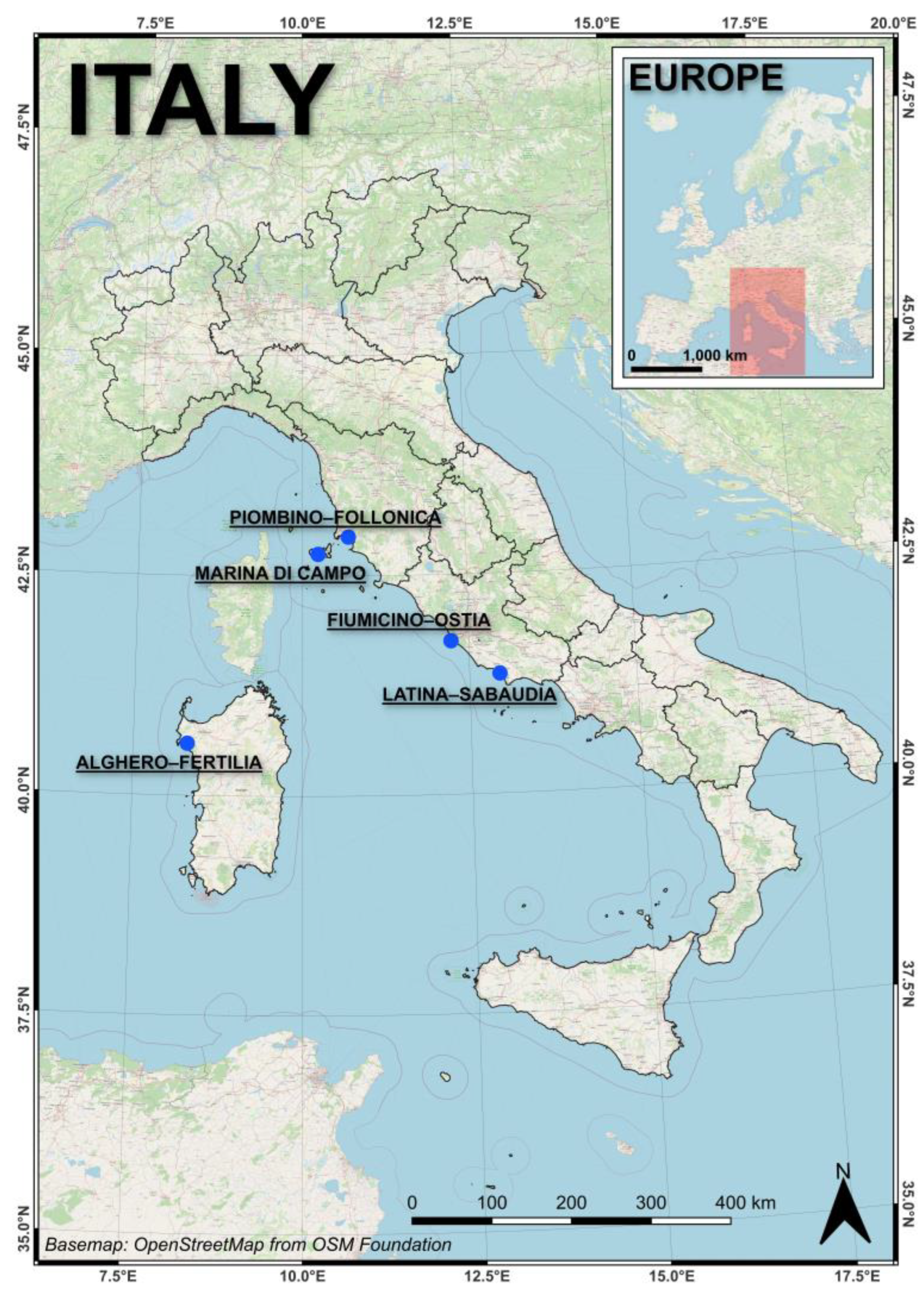
2. Study Area
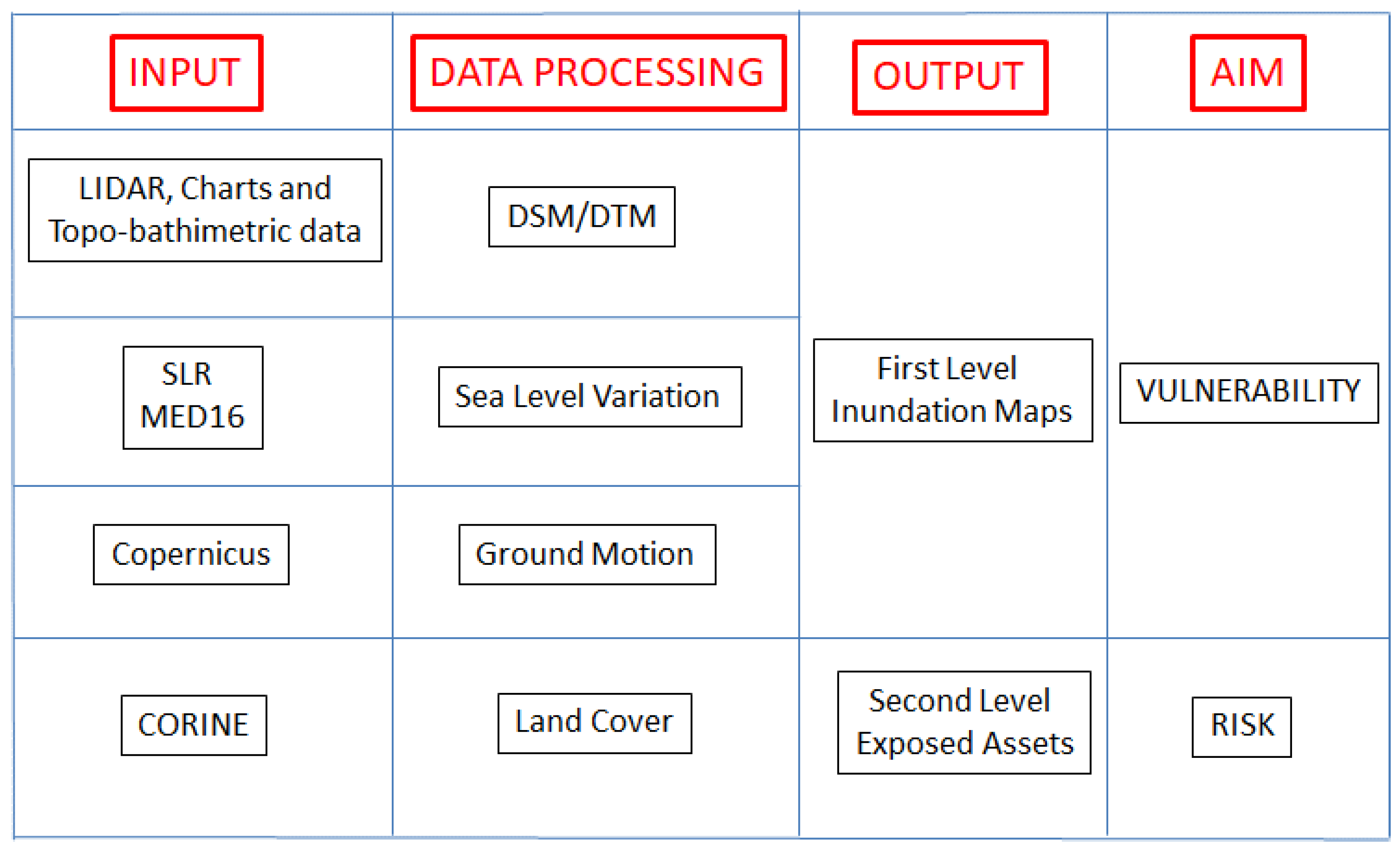
3. Data and Methodology
3.1. MED16 Ocean Model
3.2. Topography and Bathymetry
3.3. Ground Motion
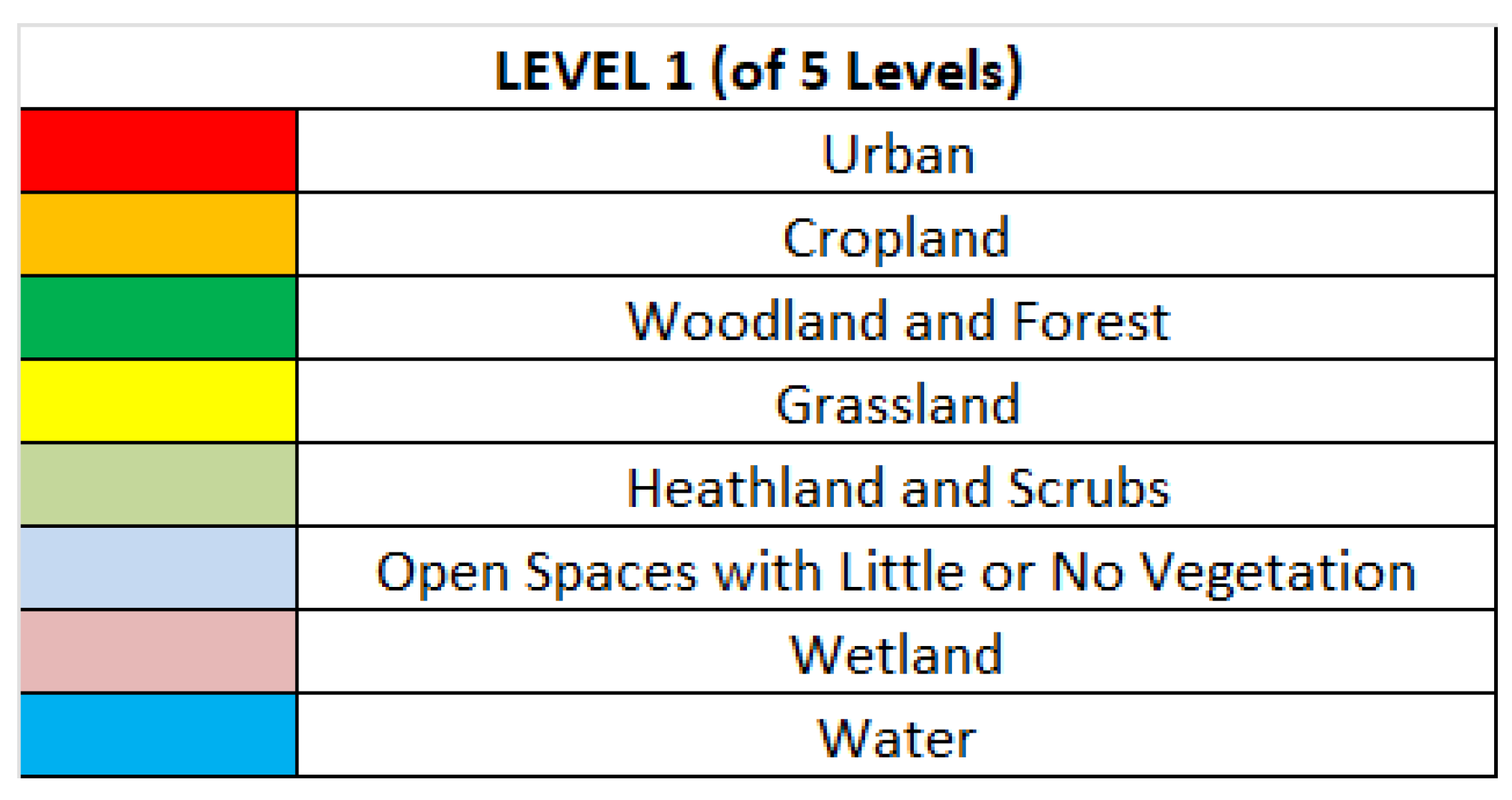
3.4. Land Cover
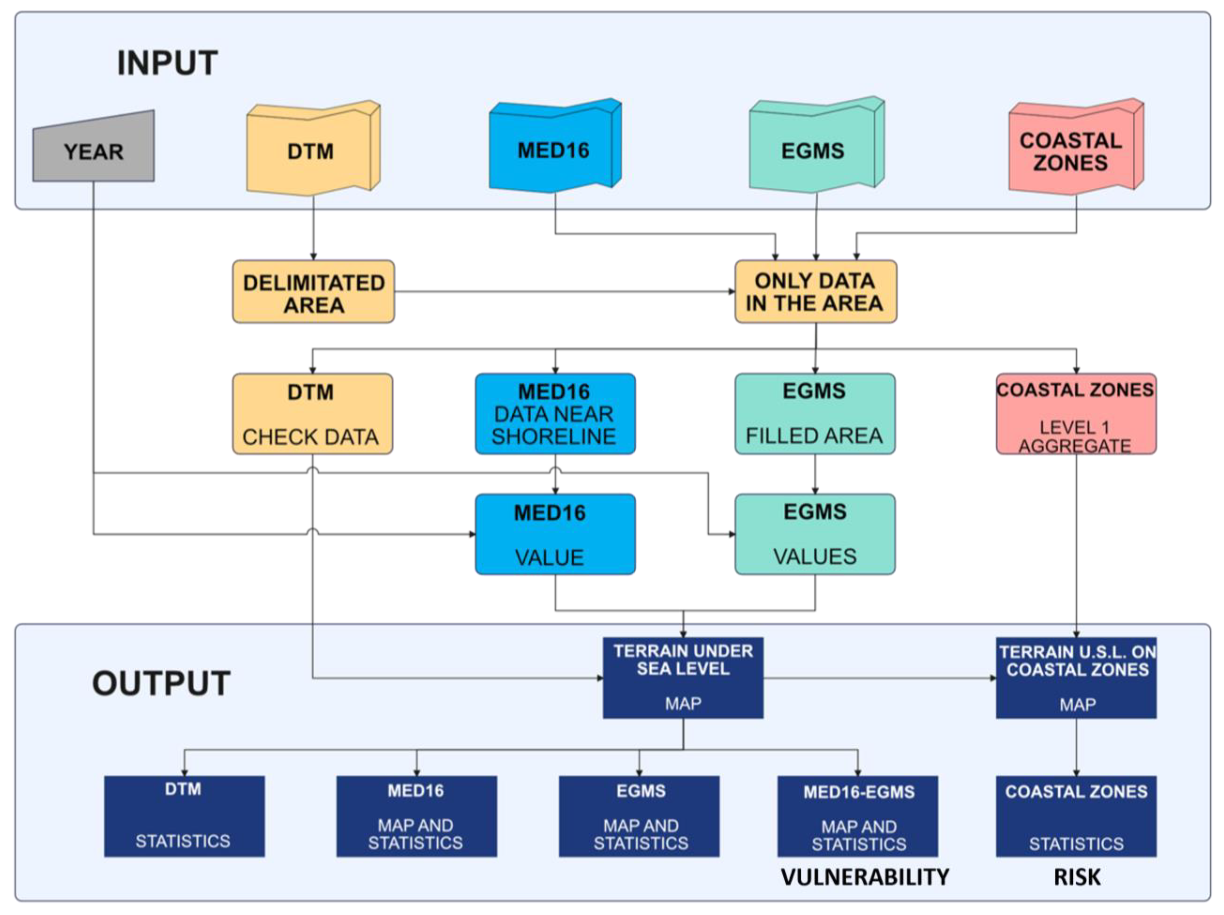
3.5. Processing Chain
4. Results
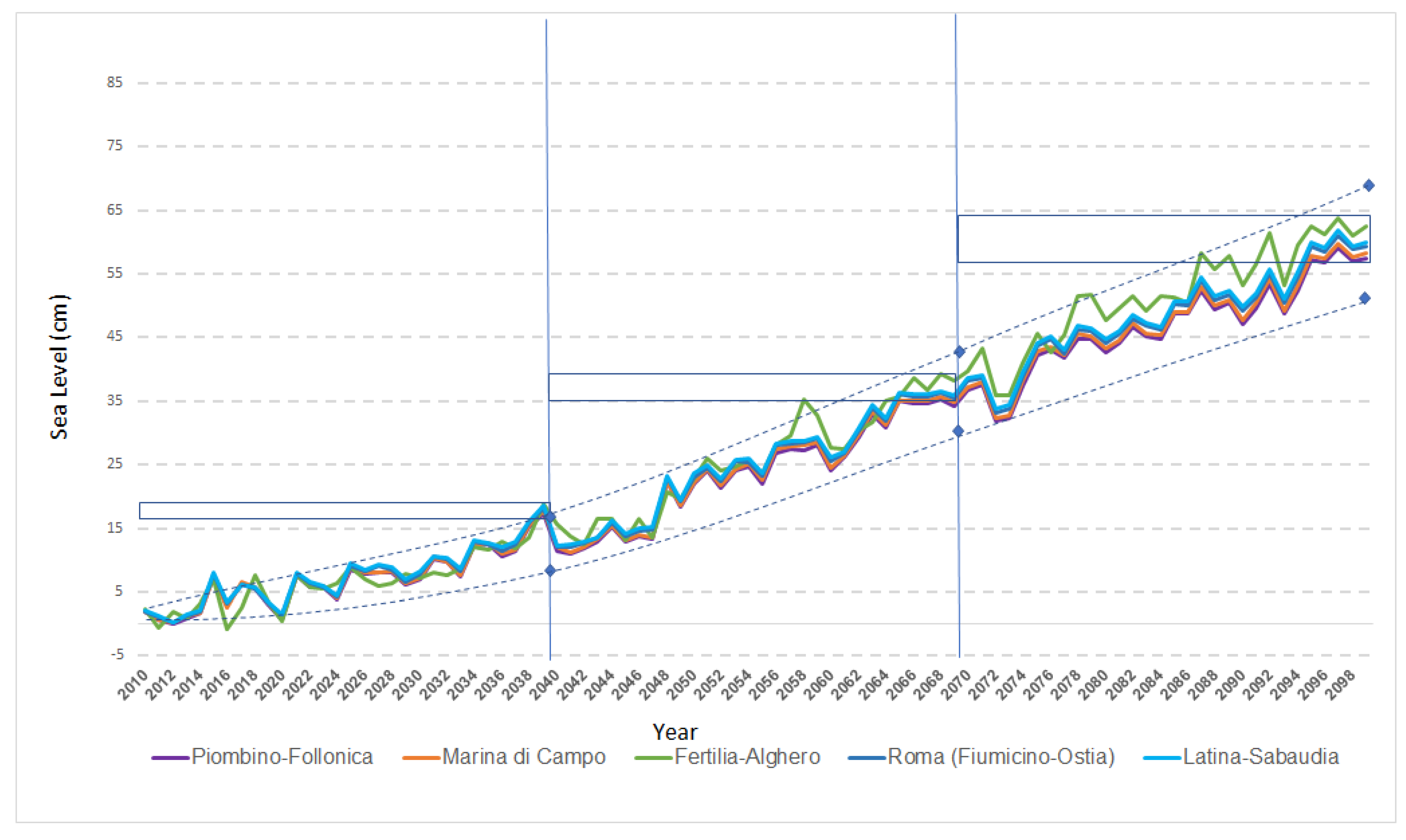
4.1. SLR in the Study Areas
4.2. Topography
4.3. Ground Motion
4.4. Inundation Maps
4.5. Assessment of Exposed Assets
5. Discussion and Conclusions
Author Contributions
Funding
Data Availability Statement
Acknowledgments
Conflicts of Interest
Abbreviations
References
- Nicholls, R.J.; Lincke, D.; Hinkel, J.; Brown, S.; Vafeidis, A.T.; Meyssignac, B.; Hanson, S.E.; Merkens, J.-L.; Fang, J. A Global Analysis of Subsidence, Relative Sea-Level Change and Coastal Flood Exposure. Nat. Clim. Chang. 2021, 11, 338–342. [Google Scholar] [CrossRef]
- Deiana, G.; Antonioli, F.; Moretti, L.; Orrù, P.E.; Randazzo, G.; Lo Presti, V. MIS 5.5 Highstand and Future Sea Level Flooding at 2100 and 2300 in Tectonically Stable Areas of Central Mediterranean Sea: Sardinia and the Pontina Plain (Southern Latium), Italy. Water 2021, 13, 2597. [Google Scholar] [CrossRef]
- Ferranti, L.; Antonioli, F.; Anzidei, M.; Monaco, C.; Stocchi, P. The Timescale and Spatial Extent of Recent Vertical Tectonic Motions in Italy: Insights from Relative Sea-Level Changes Studies. J. Virtual Explor. 2010, 36, 1–34. [Google Scholar] [CrossRef]
- Antonioli, F.; Anzidei, M.; Amorosi, A.; Lo Presti, V.; Mastronuzzi, G.; Deiana, G.; De Falco, G.; Fontana, A.; Fontolan, G.; Lisco, S.; et al. Sea-Level Rise and Potential Drowning of the Italian Coastal Plains: Flooding Risk Scenarios for 2100. Quat. Sci. Rev. 2017, 158, 29–43. [Google Scholar] [CrossRef]
- Amadio, M.; Essenfelder, A.H.; Bagli, S.; Marzi, S.; Mazzoli, P.; Mysiak, J.; Roberts, S. Cost–Benefit Analysis of Coastal Flood Defence Measures in the North Adriatic Sea. Nat. Hazards Earth Syst. Sci. 2022, 22, 265–286. [Google Scholar] [CrossRef]
- Hallegatte, S.; Green, C.; Nicholls, R.J.; Corfee-Morlot, J. Future Flood Losses in Major Coastal Cities. Nat. Clim. Chang. 2013, 3, 802–806. [Google Scholar] [CrossRef]
- Heberger, M.; Cooley, H.; Herrera, P.; Gleick, P.H.; Moore, E. Potential Impacts of Increased Coastal Flooding in California Due to Sea-Level Rise. Clim. Chang. 2011, 109, 229–249. [Google Scholar] [CrossRef]
- Paulik, R.; Wild, A.; Stephens, S.; Welsh, R.; Wadhwa, S. National Assessment of Extreme Sea-Level Driven Inundation under Rising Sea Levels. Front. Environ. Sci. 2023, 10, 1045743. [Google Scholar] [CrossRef]
- Hume, T.M.; Gerbeaux, P.; Hart, D.; Kettles, D.; Neale, D. A Classification of NZ Coastal Hydrosystems for Management Purpose; Hamilton, NIWA Client Report HAM2016-062; National Institute of Water & Atmospheric Research Ltd.: Auckland, New Zealand, 2016; p. 120. [Google Scholar]
- Kappes, M.; Keiler, M.; Glade, T. From Single- to Multi-Hazard Risk Analyses: A Concept Addressing Emerging Challenges. In Proceedings of the Mountains Risks: Bringing Science to Society, Florence, Italy, 24–26 November 2010; Malet, J.P., Glade, T., Casagli, N., Eds.; CERG Editions: Strassbourg, France, 2010; pp. 351–356. [Google Scholar]
- Kappes, M.S. Multi-Hazard Risk Analyses: A Concept and Its Implementation. Doctor Dissertation, University of Vienna, Vienna, Austria, 2011. [Google Scholar]
- Kappes, M.S.; Papathoma-Köhle, M.; Keiler, M. Assessing Physical Vulnerability for Multi-Hazards Using an Indicator-Based Methodology. Appl. Geogr. 2012, 32, 577–590. [Google Scholar] [CrossRef]
- Garner, G.; Hermans, T.H.J.; Kopp, R.; Slangen, A.; Edwards, T.; Levermann, A.; Nowicki, S.; Palmer, M.D.; Smith, C.; Fox-Kemper, B.; et al. IPCC AR6 WGI Sea Level Projections 2023; 1701334484 Bytes; IPCC: Geneva, Switzerland, 2023. [Google Scholar]
- Antonioli, F.; Silenzi, S.; Vittori, E.; Villani, C. Sea Level Changes and Tectonic Mobility: Precise Measurements in Three Coastlines of Italy Considered Stable during the Last 125 Ky. Phys. Chem. Earth Part A Solid Earth Geod. 1999, 24, 337–342. [Google Scholar] [CrossRef]
- Bonaldo, D.; Antonioli, F.; Archetti, R.; Bezzi, A.; Correggiari, A.; Davolio, S.; De Falco, G.; Fantini, M.; Fontolan, G.; Furlani, S.; et al. Integrating Multidisciplinary Instruments for Assessing Coastal Vulnerability to Erosion and Sea Level Rise: Lessons and Challenges from the Adriatic Sea, Italy. J. Coast. Conserv. 2019, 23, 19–37. [Google Scholar] [CrossRef]
- Lambeck, K.; Antonioli, F.; Purcell, A.; Silenzi, S. Sea-Level Change along the Italian Coast for the Past 10,000yr. Quat. Sci. Rev. 2004, 23, 1567–1598. [Google Scholar] [CrossRef]
- Lambeck, K.; Antonioli, F.; Anzidei, M.; Ferranti, L.; Leoni, G.; Scicchitano, G.; Silenzi, S. Sea Level Change along the Italian Coast during the Holocene and Projections for the Future. Quat. Int. 2011, 232, 250–257. [Google Scholar] [CrossRef]
- Lambeck, K.; Anzidei, M.; Antonioli, F.; Benini, A.; Esposito, A. Sea Level in Roman Time in the Central Mediterranean and Implications for Recent Change. Earth Planet. Sci. Lett. 2004, 224, 563–575. [Google Scholar] [CrossRef]
- Fox-Kemper, B.; Hewitt, H.T.; Xiao, C.; Aðalgeirsdóttir, G.; Drijfhout, S.S.; Edwards, T.L.; Golledge, N.R.; Hemer, M.; Kopp, R.E.; Krinner, G.; et al. Ocean, Cryosphere and Sea Level Change. In Climate Change 2021: The Physical Science Basis. Contribution of Working Group I to the Sixth Assessment Report of the Intergovernmental Panel on Climate Change; Masson-Delmotte, V., Zhai, P., Pirani, A., Connors, S.L., Péan, C., Berger, S., Caud, N., Chen, Y., Goldfarb, L., Gomis, M.I., et al., Eds.; Cambridge University Press: Cambridge, UK; New York, NY, USA, 2021; pp. 1211–1362. [Google Scholar] [CrossRef]
- Didier, D.; Baudry, J.; Bernatchez, P.; Dumont, D.; Sadegh, M.; Bismuth, E.; Bandet, M.; Dugas, S.; Sévigny, C. Multihazard Simulation for Coastal Flood Mapping: Bathtub versus Numerical Modelling in an Open Estuary, Eastern Canada. J. Flood Risk Manag. 2019, 12, e12505. [Google Scholar] [CrossRef]
- Cappucci, S.; Bertoni, D.; Cipriani, L.E.; Boninsegni, G.; Sarti, G. Assessment of the Anthropogenic Sediment Budget of a Littoral Cell System (Northern Tuscany, Italy). Water 2020, 12, 3240. [Google Scholar] [CrossRef]
- Spada, G.; Melini, D. New Estimates of Ongoing Sea Level Change and Land Movements Caused by Glacial Isostatic Adjustment in the Mediterranean Region. Geophys. J. Int. 2022, 229, 984–998. [Google Scholar] [CrossRef]
- Crosetto, M.; Solari, L.; Mróz, M.; Balasis-Levinsen, J.; Casagli, N.; Frei, M.; Oyen, A.; Moldestad, D.A.; Bateson, L.; Guerrieri, L.; et al. The Evolution of Wide-Area DInSAR: From Regional and National Services to the European Ground Motion Service. Remote Sens. 2020, 12, 2043. [Google Scholar] [CrossRef]
- Crosetto, M.; Solari, L.; Balasis-Levinsen, J.; Bateson, L.; Casagli, N.; Frei, M.; Oyen, A.; Moldestad, D.A.; Mróz, M. Deformation Monitoring at European Scale: The Copernicus Ground Motion Service. Int. Arch. Photogramm. Remote Sens. Spat. Inf. Sci. 2021, XLIII-B3-2021, 141–146. [Google Scholar] [CrossRef]
- Antonioli, F.; De Falco, G.; Lo Presti, V.; Moretti, L.; Scardino, G.; Anzidei, M.; Bonaldo, D.; Carniel, S.; Leoni, G.; Furlani, S.; et al. Relative Sea-Level Rise and Potential Submersion Risk for 2100 on 16 Coastal Plains of the Mediterranean Sea. Water 2020, 12, 2173. [Google Scholar] [CrossRef]
- Nicholls, R.J.; Cazenave, A. Sea-Level Rise and Its Impact on Coastal Zones. Science 2010, 328, 1517–1520. [Google Scholar] [CrossRef]
- Falciano, A.; Anzidei, M.; Greco, M.; Trivigno, M.L.; Vecchio, A.; Georgiadis, C.; Patias, P.; Crosetto, M.; Navarro, J.; Serpelloni, E.; et al. The SAVEMEDCOASTS-2 webGIS: The Online Platform for Relative Sea Level Rise and Storm Surge Scenarios up to 2100 for the Mediterranean Coasts. J. Mar. Sci. Eng. 2023, 11, 2071. [Google Scholar] [CrossRef]
- Andreucci, S.; Santonastaso, A.; De Luca, M.; Cappucci, S.; Cucco, A.; Quattrocchi, G.; Pascucci, V. A Shallow-Water Dunefield in a Microtidal, Wind-Dominated Strait (Stintino, NW Sardinia, Italy). Geol. Soc. Lond. Spéc. Publ. 2023, 523, 173–194. [Google Scholar] [CrossRef]
- Moftakhari, H.R.; AghaKouchak, A.; Sanders, B.F.; Feldman, D.L.; Sweet, W.; Matthew, R.A.; Luke, A. Increased Nuisance Flooding along the Coasts of the United States Due to Sea Level Rise: Past and Future. Geophys. Res. Lett. 2015, 42, 9846–9852. [Google Scholar] [CrossRef]
- Zanchettin, D.; Rubinetti, S.; Rubino, A. Is the Atlantic a Source for Decadal Predictability of Sea-Level Rise in Venice? Earth Space Sci. 2022, 9, e2022EA002494. [Google Scholar] [CrossRef]
- Ward, P.J.; Couasnon, A.; Eilander, D.; Haigh, I.D.; Hendry, A.; Muis, S.; Veldkamp, T.I.E.; Winsemius, H.C.; Wahl, T. Dependence between High Sea-Level and High River Discharge Increases Flood Hazard in Global Deltas and Estuaries. Environ. Res. Lett. 2018, 13, 084012. [Google Scholar] [CrossRef]
- Thiéblemont, R.; Le Cozannet, G.; D’Anna, M.; Idier, D.; Belmadani, A.; Slangen, A.B.A.; Longueville, F. Chronic Flooding Events Due to Sea-Level Rise in French Guiana. Sci. Rep. 2023, 13, 21695. [Google Scholar] [CrossRef]
- Vousdoukas, M.I.; Voukouvalas, E.; Mentaschi, L.; Dottori, F.; Giardino, A.; Bouziotas, D.; Bianchi, A.; Salamon, P.; Feyen, L. Developments in Large-Scale Coastal Flood Hazard Mapping. Nat. Hazards Earth Syst. Sci. 2016, 16, 1841–1853. [Google Scholar] [CrossRef]
- Acciarri, A.; Bisci, C.; Cantalamessa, G.; Cappucci, S.; Conti, M.; Di Pancrazio, G.; Spagnoli, F.; Valentini, E. Metrics for Short-Term Coastal Characterization, Protection and Planning Decisions of Sentina Natural Reserve, Italy. Ocean Coast. Manag. 2021, 201, 105472. [Google Scholar] [CrossRef]
- Luijendijk, A.; Hagenaars, G.; Ranasinghe, R.; Baart, F.; Donchyts, G.; Aarninkhof, S. The State of the World’s Beaches. Sci. Rep. 2018, 8, 6641. [Google Scholar] [CrossRef] [PubMed]
- Shadrick, J.R.; Rood, D.H.; Hurst, M.D.; Piggott, M.D.; Hebditch, B.G.; Seal, A.J.; Wilcken, K.M. Sea-Level Rise Will Likely Accelerate Rock Coast Cliff Retreat Rates. Nat. Commun. 2022, 13, 7005. [Google Scholar] [CrossRef] [PubMed]
- Becker, M.; Karpytchev, M.; Hu, A. Increased Exposure of Coastal Cities to Sea-Level Rise Due to Internal Climate Variability. Nat. Clim. Chang. 2023, 13, 367–374. [Google Scholar] [CrossRef]
- Jiménez, J.; Armaroli, C.; Bosom, E. Preparing for the Impact of Coastal Storms: A Coastal Manager-oriented Approach. In Coastal Storms; Ciavola, P., Coco, G., Eds.; Wiley: Hoboken, NJ, USA, 2017; pp. 217–239. ISBN 978-1-118-93710-5. [Google Scholar]
- Le Cozannet, G.; Nicholls, R.; Hinkel, J.; Sweet, W.; McInnes, K.; Van De Wal, R.; Slangen, A.; Lowe, J.; White, K. Sea Level Change and Coastal Climate Services: The Way Forward. J. Mar. Sci. Eng. 2017, 5, 49. [Google Scholar] [CrossRef]
- Wadey, M.P.; Nicholls, R.J.; Haigh, I. Understanding a Coastal Flood Event: The 10th March 2008 Storm Surge Event in the Solent, UK. Nat. Hazards 2013, 67, 829–854. [Google Scholar] [CrossRef]
- Ward, P.J.; Jongman, B.; Aerts, J.C.J.H.; Bates, P.D.; Botzen, W.J.W.; Diaz Loaiza, A.; Hallegatte, S.; Kind, J.M.; Kwadijk, J.; Scussolini, P.; et al. A Global Framework for Future Costs and Benefits of River-Flood Protection in Urban Areas. Nat. Clim. Chang. 2017, 7, 642–646. [Google Scholar] [CrossRef]
- Ward, P.J.; Blauhut, V.; Bloemendaal, N.; Daniell, J.E.; De Ruiter, M.C.; Duncan, M.J.; Emberson, R.; Jenkins, S.F.; Kirschbaum, D.; Kunz, M.; et al. Review Article: Natural Hazard Risk Assessments at the Global Scale. Nat. Hazards Earth Syst. Sci. 2020, 20, 1069–1096. [Google Scholar] [CrossRef]
- Kulp, S.A.; Strauss, B.H. CoastalDEM: A Global Coastal Digital Elevation Model Improved from SRTM Using a Neural Network. Remote Sens. Environ. 2018, 206, 231–239. [Google Scholar] [CrossRef]
- Kulp, S.A.; Strauss, B.H. New Elevation Data Triple Estimates of Global Vulnerability to Sea-Level Rise and Coastal Flooding. Nat. Commun. 2019, 10, 4844. [Google Scholar] [CrossRef] [PubMed]
- Hinkel, J.; Church, J.A.; Gregory, J.M.; Lambert, E.; Le Cozannet, G.; Lowe, J.; McInnes, K.L.; Nicholls, R.J.; Van Der Pol, T.D.; Van De Wal, R. Meeting User Needs for Sea Level Rise Information: A Decision Analysis Perspective. Earth’s Future 2019, 7, 320–337. [Google Scholar] [CrossRef]
- Oppenheimer, M.; Glavovic, B.C.; Hinkel, J.; van de Wal, R.; Magnan, A.K.; Abd-EIgawad, A.; Cai, R.; Cifuentes-Jara, M.; DeConto, R.M.; Ghosh, T.; et al. Sea Level Rise and Implications for Low-Lying Islands, Coasts and Communities; Intergovernmental Panel on Climate Change: Geneva, Switzerland, 2019; p. 126. [Google Scholar]
- Hinkel, J.; Lincke, D.; Vafeidis, A.T.; Perrette, M.; Nicholls, R.J.; Tol, R.S.J.; Marzeion, B.; Fettweis, X.; Ionescu, C.; Levermann, A. Coastal Flood Damage and Adaptation Costs under 21st Century Sea-Level Rise. Proc. Natl. Acad. Sci. USA 2014, 111, 3292–3297. [Google Scholar] [CrossRef]
- Hinkel, J.; Jaeger, C.; Nicholls, R.J.; Lowe, J.; Renn, O.; Peijun, S. Sea-Level Rise Scenarios and Coastal Risk Management. Nat. Clim. Chang. 2015, 5, 188–190. [Google Scholar] [CrossRef]
- Wilkinson, M.D.; Dumontier, M.; Aalbersberg, I.J.; Appleton, G.; Axton, M.; Baak, A.; Blomberg, N.; Boiten, J.-W.; Da Silva Santos, L.B.; Bourne, P.E.; et al. The FAIR Guiding Principles for Scientific Data Management and Stewardship. Sci. Data 2016, 3, 160018. [Google Scholar] [CrossRef]
- Tellez-Arenas, A.; Quique, R.; Boulahya, F.; Le Cozannet, G.; Paris, F.; Leroy, S.; Dupros, F.; Robida, F. Scalable Interactive Platform for Geographic Evaluation of Sea-Level Rise Impact Combining High-Performance Computing and WebGIS Client; HAL Open Science: Lyon, France, 2018. [Google Scholar]
- Gesch, D.B. Best Practices for Elevation-Based Assessments of Sea-Level Rise and Coastal Flooding Exposure. Front. Earth Sci. 2018, 6, 230. [Google Scholar] [CrossRef]
- SaveCoast. Available online: https://savecoast.com/en/home-en/ (accessed on 30 April 2024).
- CoCliCo Project H2020. Available online: https://cordis.europa.eu/project/id/101003598 (accessed on 30 April 2024).
- Seibold, E. Natural Disasters and Early Warning. In Early Warning Systems for Natural Disaster Reduction; Zschau, J., Küppers, A., Eds.; Springer: Berlin/Heidelberg, Germany, 2003; pp. 3–10. ISBN 978-3-642-63234-1. [Google Scholar]
- Tilloy, A.; Malamud, B.D.; Winter, H.; Joly-Laugel, A. A Review of Quantification Methodologies for Multi-Hazard Interrelationships. Earth-Sci. Rev. 2019, 196, 102881. [Google Scholar] [CrossRef]
- Barnard, P.L.; Short, A.D.; Harley, M.D.; Splinter, K.D.; Vitousek, S.; Turner, I.L.; Allan, J.; Banno, M.; Bryan, K.R.; Doria, A.; et al. Coastal Vulnerability across the Pacific Dominated by El Niño/Southern Oscillation. Nat. Geosci. 2015, 8, 801–807. [Google Scholar] [CrossRef]
- Jorissen, R.; Kraaij, E.; Tromp, E. Dutch Flood Protection Policy and Measures Based on Risk Assessment. E3S Web Conf. 2016, 7, 20016. [Google Scholar] [CrossRef]
- Ward, P.J.; Jongman, B.; Weiland, F.S.; Bouwman, A.; Van Beek, R.; Bierkens, M.F.P.; Ligtvoet, W.; Winsemius, H.C. Assessing Flood Risk at the Global Scale: Model Setup, Results, and Sensitivity. Environ. Res. Lett. 2013, 8, 044019. [Google Scholar] [CrossRef]
- Ward, P.J.; Kummu, M.; Lall, U. Flood Frequencies and Durations and Their Response to El Niño Southern Oscillation: Global Analysis. J. Hydrol. 2016, 539, 358–378. [Google Scholar] [CrossRef]
- Sánchez Garrido, J.C.; García Lafuente, J.; Criado Aldeanueva, F.; Baquerizo, A.; Sannino, G. Time-spatial Variability Observed in Velocity of Propagation of the Internal Bore in the Strait of Gibraltar. J. Geophys. Res. 2008, 113, 2007JC004624. [Google Scholar] [CrossRef]
- Sannino, G.; Bargagli, A.; Artale, V. Numerical Modeling of the Semidiurnal Tidal Exchange through the Strait of Gibraltar. J. Geophys. Res. 2004, 109, 2003JC002057. [Google Scholar] [CrossRef]
- Sannino, G.; Carillo, A.; Artale, V. Three-layer View of Transports and Hydraulics in the Strait of Gibraltar: A Three-dimensional Model Study. J. Geophys. Res. 2007, 112, 2006JC003717. [Google Scholar] [CrossRef]
- Sannino, G.; Pratt, L.; Carillo, A. Hydraulic Criticality of the Exchange Flow through the Strait of Gibraltar. J. Phys. Oceanogr. 2009, 39, 2779–2799. [Google Scholar] [CrossRef]
- Gonzalez, N.M.; Waldman, R.; Sannino, G.; Giordani, H.; Somot, S. Understanding Tidal Mixing at the Strait of Gibraltar: A High-Resolution Model Approach. Prog. Oceanogr. 2023, 212, 102980. [Google Scholar] [CrossRef]
- Artale, V.; The PROTHEUS Group; Calmanti, S.; Carillo, A.; Dell’Aquila, A.; Herrmann, M.; Pisacane, G.; Ruti, P.M.; Sannino, G.; Struglia, M.V.; et al. An Atmosphere–Ocean Regional Climate Model for the Mediterranean Area: Assessment of a Present Climate Simulation. Clim. Dyn. 2010, 35, 721–740. [Google Scholar] [CrossRef]
- Sannino, G.; Carillo, A.; Pisacane, G.; Naranjo, C. On the Relevance of Tidal Forcing in Modelling the Mediterranean Thermohaline Circulation. Prog. Oceanogr. 2015, 134, 304–329. [Google Scholar] [CrossRef]
- Akhtar, N.; Brauch, J.; Ahrens, B. Climate Modeling over the Mediterranean Sea: Impact of Resolution and Ocean Coupling. Clim. Dyn. 2018, 51, 933–948. [Google Scholar] [CrossRef]
- Nabat, P.; Somot, S.; Cassou, C.; Mallet, M.; Michou, M.; Bouniol, D.; Decharme, B.; Drugé, T.; Roehrig, R.; Saint-Martin, D. Modulation of Radiative Aerosols Effects by Atmospheric Circulation over the Euro-Mediterranean Region. Atmos. Chem. Phys. 2020, 20, 8315–8349. [Google Scholar] [CrossRef]
- Reale, M.; Giorgi, F.; Solidoro, C.; Di Biagio, V.; Di Sante, F.; Mariotti, L.; Farneti, R.; Sannino, G. The Regional Earth System Model RegCM-ES: Evaluation of the Mediterranean Climate and Marine Biogeochemistry. J. Adv. Model. Earth Syst. 2020, 12, e2019MS001812. [Google Scholar] [CrossRef]
- Anav, A.; Carillo, A.; Palma, M.; Struglia, M.V.; Turuncoglu, U.U.; Sannino, G. The ENEA-REG System (v1.0), a Multi-Component Regional Earth System Model: Sensitivity to Different Atmospheric Components over the Med-CORDEX (Coordinated Regional Climate Downscaling Experiment) Region. Geosci. Model Dev. 2021, 14, 4159–4185. [Google Scholar] [CrossRef]
- Adloff, F.; Jordà, G.; Somot, S.; Sevault, F.; Arsouze, T.; Meyssignac, B.; Li, L.; Planton, S. Improving Sea Level Simulation in Mediterranean Regional Climate Models. Clim. Dyn. 2018, 51, 1167–1178. [Google Scholar] [CrossRef]
- Sannino, G.; Carillo, A.; Iacono, R.; Napolitano, E.; Palma, M.; Pisacane, G.; Struglia, M. Modelling Present and Future Climate in the Mediterranean Sea: A Focus on Sea-Level Change. Clim. Dyn. 2022, 59, 357–391. [Google Scholar] [CrossRef]
- Allison, M.; Yuill, B.; Törnqvist, T.; Amelung, F.; Dixon, T.; Erkens, G.; Stuurman, R.; Jones, C.; Milne, G.; Steckler, M.; et al. Global Risks and Research Priorities for Coastal Subsidence. Eos 2016, 97, 22–27. [Google Scholar] [CrossRef]
- King, B.A.; Blackley, M.W.L.; Carr, A.P.; Hardcastle, P.J. Observations of Wave-induced Set-up on a Natural Beach. J. Geophys. Res. 1990, 95, 22289–22297. [Google Scholar] [CrossRef]
- Ramirez, J.A.; Lichter, M.; Coulthard, T.J.; Skinner, C. Hyper-Resolution Mapping of Regional Storm Surge and Tide Flooding: Comparison of Static and Dynamic Models. Nat. Hazards 2016, 82, 571–590. [Google Scholar] [CrossRef]
- Cappucci, S.; De Cassan, M.; Grillini, M.; Proposito, M.; Screpanti, A. Multisource water characterisation for water supply and management strategies on a small Mediterranean Island. Hydrogeol. J. 2020, 28, 1155–1171. [Google Scholar] [CrossRef]
- Aerts, J.C.J.H.; Barnard, P.L.; Botzen, W.; Grifman, P.; Hart, J.F.; De Moel, H.; Mann, A.N.; De Ruig, L.T.; Sadrpour, N. Pathways to Resilience: Adapting to Sea Level Rise in Los Angeles. Ann. N. Y. Acad. Sci. 2018, 1427, 1–90. [Google Scholar] [CrossRef] [PubMed]
- Sayers, P.; Galloway, G.; Penning-Rowsell, E.; Yuanyuan, L.; Fuxin, S.; Yiwei, C.; Kang, W.; Le Quesne, T.; Wang, L.; Guan, Y. Strategic Flood Management: Ten ‘Golden Rules’ to Guide a Sound Approach. Int. J. River Basin Manag. 2015, 13, 137–151. [Google Scholar] [CrossRef]
- Motta Zanin, G.; Barbanente, A.; Romagnoli, C.; Parisi, A.; Archetti, R. Traditional vs. novel approaches to coastal risk management: A review and insights from Italy. J. Environ. Manag. 2023, 346, 119003. [Google Scholar] [CrossRef]
- Cipriani, L.E.; Pranzini, E.; Vitale, G. Coastal erosion in Tuscany: Short vs. medium term evolution. In Coastal Erosion Monitoring. A Network of Regional Observatories—Results from RESMAR Project; Cipriani, L.E., Ed.; Nuova Grafica Fiorentina: Florence, Italy, 2013; pp. 135–155. [Google Scholar]
- Pranzini, E.; Cinelli, I.; Cipriani, L.E.; Anfuso, G. An Integrated Coastal Sediment Management Plan: The Example of the Tuscany Region (Italy). J. Mar. Sci. Eng. 2020, 8, 33. [Google Scholar] [CrossRef]
- Bigongiari, N.; Cipriani, L.E.; Pranzini, E.; Renzi, M.; Vitale, G. Assessing Shelf Aggregate Environmental Compatibility and Suitability for Beach Nourishment: A Case Study for Tuscany (Italy). Mar. Pollut. Bull. 2015, 93, 183–193. [Google Scholar] [CrossRef]
- Pranzini, E.; Anfuso, G.; Cinelli, I.; Piccardi, M.; Vitale, G. Shore Protection Structures Increase and Evolution on the Northern Tuscany Coast (Italy): Influence of Tourism Industry. Water 2018, 10, 1647. [Google Scholar] [CrossRef]
- Cappucci, S.; Vaccari, M.; Falconi, M.; Tudor, T. Sustainable Management of Sedimentary Resources: A Case Study of the Egadi Project. Environ. Eng. Manag. J. 2019, 18, 317–328. [Google Scholar]
- Iacono, R.; Napolitano, E.; Palma, M.; Sannino, G. The Tyrrhenian Sea Circulation: A Review of Recent Work. Sustainability 2021, 13, 6371. [Google Scholar] [CrossRef]
- Bendoni, M.; Fattorini, M.; Taddei, S.; Brandini, C. High-Resolution Downscaling of CMEMS Oceanographic Reanalysis in the Area of the Tuscany Archipelago (Italy). Ocean Dyn. 2022, 72, 295–312. [Google Scholar] [CrossRef]
- Ciuffardi, T.; Napolitano, E.; Iacono, R.; Reseghetti, F.; Raiteri, G.; Bordone, A. Analysis of Surface Circulation Structures along a Frequently Repeated XBT Transect Crossing the Ligurian and Tyrrhenian Seas. Ocean Dyn. 2016, 66, 767–783. [Google Scholar] [CrossRef]
- Iacono, R.; Napolitano, E. Aspects of the Summer Circulation in the Eastern Ligurian Sea. Deep Sea Res. Part I Oceanogr. Res. Pap. 2020, 166, 103407. [Google Scholar] [CrossRef]
- Manca, E.; Pascucci, V.; Deluca, M.; Cossu, A.; Andreucci, S. Shoreline Evolution Related to Coastal Development of a Managed Beach in Alghero, Sardinia, Italy. Ocean Coast. Manag. 2013, 85, 65–76. [Google Scholar] [CrossRef]
- De Luca, M.; Pascucci, V.; Puccini, A.; Pireddu, L.; Santonastaso, A.; Stelletti, M.; Gazale, V.; Zanello, A. Sea Floorof the Marine Protected Area of the Asinara Island (Sardinia, Italy). J. Maps 2022, 18, 288–299. [Google Scholar] [CrossRef]
- Vicinanza, D.; Contestabile, P.; Ferrante, V. Wave Energy Potential in the North-West of Sardinia (Italy). Renew. Energy 2013, 50, 506–521. [Google Scholar] [CrossRef]
- Pallottini, E.; Cappucci, S. Beach-dune system interaction and evolution. Rend. Online Soc. Geol. Ital. 2009, 8, 87–97. [Google Scholar]
- Valentini, E.; Taramelli, A.; Cappucci, S.; Filipponi, F.; Nguyen Xuan, A. Exploring the Dunes: The Correlations between Vegetation Cover Pattern and Morphology for Sediment Retention Assessment Using Airborne Multisensor Acquisition. Remote Sens. 2020, 12, 1229. [Google Scholar] [CrossRef]
- Taramelli, A.; Cappucci, S.; Valentini, E.; Rossi, L.; Lisi, I. Nearshore Sandbar Classification of Sabaudia (Italy) with LiDAR Data: The FHyL Approach. Remote Sens. 2020, 12, 1053. [Google Scholar] [CrossRef]
- Conti, M.; Cappucci, S.; La Monica, G.B. Sediment dynamic of nourished sandy beaches. Rend. Online Soc. Geol. Ital. 2009, 8, 31–38. [Google Scholar]
- Marshall, J.; Hill, C.; Perelman, L.; Adcroft, A. Hydrostatic, Quasi-hydrostatic, and Nonhydrostatic Ocean Modeling. J. Geophys. Res. 1997, 102, 5733–5752. [Google Scholar] [CrossRef]
- Strandberg, G.; Bärring, L.; Hansson, U.; Jansson, C.; Jones, C.; Kjellström, E.; Kolax, M.; Kupiainen, M.; Nikulin, G.; Samuelsson, P.; et al. CORDEX Scenarios for Europe from the Rossby Centre Regional Climate Model RCA4; Report Meteorology and Climatology; SMHI: Norrköping, Sweden, 2014; Volume 116, p. 84. [Google Scholar]
- Dee, D.P.; Uppala, S.M.; Simmons, A.J.; Berrisford, P.; Poli, P.; Kobayashi, S.; Andrae, U.; Balmaseda, M.A.; Balsamo, G.; Bauer, P.; et al. The ERA-Interim Reanalysis: Configuration and Performance of the Data Assimilation System. Q. J. R. Meteorol. Soc. 2011, 137, 553–597. [Google Scholar] [CrossRef]
- Collins, W.J.; Bellouin, N.; Doutriaux-Boucher, M.; Gedney, N.; Halloran, P.; Hinton, T.; Hughes, J.; Jones, C.D.; Joshi, M.; Liddicoat, S.; et al. Development and Evaluation of an Earth-System Model—HadGEM2. Geosci. Model Dev. 2011, 4, 1051–1075. [Google Scholar] [CrossRef]
- Cappucci, S.; Valentini, E.; Monte, M.D.; Paci, M.; Filipponi, F.; Taramelli, A. Detection of Natural and Anthropic Features on Small Islands. J. Coast. Res. 2017, 77, 73–87. [Google Scholar] [CrossRef]
- Gallien, T.W.; Barnard, P.L.; Van Ormondt, M.; Foxgrover, A.C.; Sanders, B.F. A Parcel-Scale Coastal Flood Forecasting Prototype for a Southern California Urbanized Embayment. J. Coast. Res. 2012, 29, 642. [Google Scholar] [CrossRef]
- Geoportale MASE. Available online: https://gn.mase.gov.it/portale (accessed on 1 May 2024).
- Pallottini, E.; Cappucci, S.; Taramelli, A.; Innocenti, C.; Screpanti, A. Variazioni morfologiche stagionali del sistema spiaggia-duna del Parco Nazionale del Circeo. Studi Costieri 2011, 17, 105–124. [Google Scholar]
- Pedretti, L.; Bordoni, M.; Vivaldi, V.; Figini, S.; Parnigoni, M.; Grossi, A.; Lanteri, L.; Tararbra, M.; Negro, N.; Meisina, C. InterpolatiON of InSAR Time Series for the dEtection of Ground deforMatiOn eVEnts (ONtheMOVE): Application to Slow-Moving Landslides. Landslides 2023, 20, 1797–1813. [Google Scholar] [CrossRef]
- Mitáš, L.; Mitášová, H. Spatial Interpolation. Rev. Mod. Phys. 1999, 73, 33–83. [Google Scholar] [CrossRef]
- Mitasova, H.; Mitas, L.; Brown, W.M.; Gerdes, D.P.; Kosinovsky, I.; Baker, T. Modelling Spatially and Temporally Distributed Phenomena: New Methods and Tools for GRASS GIS. Int. J. Geogr. Inf. Syst. 1995, 9, 433–446. [Google Scholar] [CrossRef]
- R.Fillnulls—GRASS GIS Manual. Available online: https://grass.osgeo.org/grass83/manuals/r.fillnulls.html (accessed on 30 April 2024).
- Mitášová, H.; Mitáš, L. Interpolation by Regularized Spline with Tension: I. Theory and Implementation. Math. Geol. 1993, 25, 641–655. [Google Scholar] [CrossRef]
- Mitášová, H.; Hofierka, J. Interpolation by Regularized Spline with Tension: II. Application to Terrain Modeling and Surface Geometry Analysis. Math. Geol. 1993, 25, 657–669. [Google Scholar] [CrossRef]
- Heymann, Y. (Ed.) CORINE Land Cover: Technical Guide; Office for Official Publications of the European Communities: Luxembourg, 1994; ISBN 978-92-826-2578-1. [Google Scholar]
- Büttner, S.H.; Isemonger, E.W.; Isaacs, M.; Van Niekerk, D.; Sipler, R.E.; Dorrington, R.A. Living Phosphatic Stromatolites in a Low-phosphorus Environment: Implications for the Use of Phosphorus as a Proxy for Phosphate Levels in Paleo-systems. Geobiology 2021, 19, 35–47. [Google Scholar] [CrossRef] [PubMed]
- Coastal Zones. Available online: https://land.copernicus.eu/en/products/coastal-zones (accessed on 1 May 2024).
- Gallien, T.W.; Sanders, B.F.; Flick, R.E. Urban Coastal Flood Prediction: Integrating Wave Overtopping, Flood Defenses and Drainage. Coast. Eng. 2014, 91, 18–28. [Google Scholar] [CrossRef]
- Williams, L.L.; Lück-Vogel, M. Comparative Assessment of the GIS Based Bathtub Model and an Enhanced Bathtub Model for Coastal Inundation. J. Coast. Conserv. 2020, 24, 23. [Google Scholar] [CrossRef]
- Gomarasca, M.A.; Tornato, A.; Spizzichino, D.; Valentini, E.; Taramelli, A.; Satalino, G.; Vincini, M.; Boschetti, M.; Colombo, R.; Rossi, L.; et al. Sentinel for applications in agriculture. Int. Arch. Photogramm. Remote Sens. Spat. Inf. Sci. 2019, XLII-3/W6, 91–98. [Google Scholar] [CrossRef]
- Valentini, E.; Filipponi, F.; Xuan, A.N.; Taramelli, A. Marine food provision ecosystem services assessment using EO products. In Proceedings of the Living Planet Symposium 2016, Prague, Czech Republic, 9–13 May 2016. [Google Scholar]
- Rahmstorf, S. A Semi-Empirical Approach to Projecting Future Sea-Level Rise. Science 2007, 315, 368–370. [Google Scholar] [CrossRef]
- AR5 Climate Change 2013: The Physical Science Basis—IPCC. Available online: https://www.ipcc.ch/report/ar5/wg1/ (accessed on 1 May 2024).
- PNRR MER. Available online: https://www.isprambiente.gov.it/it/progetti/cartella-progetti-in-corso/progetti-mare/pnrr-mer-marine-ecosystem-restoration (accessed on 6 May 2024).
- Cappucci, S.; Carillo, A.; Iacono, R.; Moretti, L.; Palma, M.; Peloso, A.; Righini, S.G. Security of Mediterranean coastal areas under future inundation scenarios. In Proceedings of the Special Issue of Climate Change and Security in the Maritime Domain Conference 2023, Lerici, Italy, 3–5 October 2023. [Google Scholar]
- Joubert-Boitat, I.; Wania, A.; Dalmasso, S. Manual for CEMS-Rapid Mapping Products; EUR 30370 EN; Publications Office of the European Union: Ispra, Italy, 2020; ISBN 978-92-76-21683-4. [Google Scholar] [CrossRef]
- Wania, A.; Joubert-Boitat, I.; Dottori, F.; Kalas, M.; Salamon, P. Increasing Timeliness of Satellite-Based Flood Mapping Using Early Warning Systems in the Copernicus Emergency Management Service. Remote Sens. 2021, 13, 2114. [Google Scholar] [CrossRef]
- Antonioli, F.; Agate, A.; Ascione, A.; Cerrone, P.; Deiana, G.; Ferranti, L.; Fontana, A.; Leoni, G.; Monaco, C.; Mastronuzzi, G.; et al. Quaternary Map of Italy (Metiq); MIS 5.5 Higstand. Metiq; ISPRA, CNR, INGV, OGS, AIQUA, Eds.; Italian Geological Survey: Rome, Italy, 2023. [Google Scholar]
- Cardello, G.L.; Antonioli, F.; Barreca, G.; Monaco, C. A first comparison of instrumental European Grand Motion Service by Copernicus data with short and long term geological vertical movements for the Italian coasts. In Proceedings of the Abstract Volume INQUA Roma Congress, Rome, Italy, 13–20 July 2023; pp. 105–107. [Google Scholar]
- Cardello, G.L.; Vico, G.; Consorti, L.; Sabbatino, M.; Carminati, E.; Doglioni, C. Constraining the Passive to Active Margin Tectonics of the Internal Central Apennines: Insights from Biostratigraphy, Structural, and Seismic Analysis. Geosciences 2021, 11, 160. [Google Scholar] [CrossRef]
- Cardello, G.L.; Barreca, G.; Monaco, C.; De Michele, M.; Antonioli, F. First Comparison of Instrumental European Ground Motion Service by Copernicus Data with Short and Long-term Geological Vertical Movements for the Italian Coasts. In Proceedings of the Book of Abstract of SGI-SIMP 2024 Congress, Bari, Italy, 2–5 September 2024. [Google Scholar]
- Ferranti, L.; Antonioli, F.; Mauz, B.; Amorosi, A.; Dai Pra, G.; Mastronuzzi, G.; Monaco, C.; Orrù, P.; Pappalardo, M.; Radtke, U.; et al. Markers of the Last Interglacial Sea-Level High Stand along the Coast of Italy: Tectonic Implications. Quat. Int. 2006, 145–146, 30–54. [Google Scholar] [CrossRef]
- Antonioli, F.; Ferranti, L.; Fontana, A.; Amorosi, A.; Bondesan, A.; Braitenberg, C.; Dutton, A.; Fontolan, G.; Furlani, S.; Lambeck, K.; et al. Holocene Relative Sea-Level Changes and Vertical Movements along the Italian and Istrian Coastlines. Quat. Int. 2009, 206, 102–133. [Google Scholar] [CrossRef]
- Anav, A.; Antonelli, M.; Calmanti, S.; Carillo, A.; Catalano, F.; Dell’Aquila, A.; Iacono, R.; Marullo, S.; Napolitano, E.; Palma, M.; et al. Dynamical Downscaling of CMIP6 Scenarios with ENEA-REG: An Impact-Oriented Application for the Med-CORDEX Region. Clim. Dyn. 2024, 62, 3261–3287. [Google Scholar] [CrossRef]
- Storto, A.; Hesham Essa, Y.; De Toma, V.; Anav, A.; Sannino, G.; Santoleri, R.; Yang, C. MESMAR v1: A New Regional Coupled Climate Model for Downscaling, Predictability, and Data Assimilation Studies in the Mediterranean Region. Geosci. Model Dev. 2023, 16, 4811–4833. [Google Scholar] [CrossRef]
- Sweet, W.V.; Horton, R.; Kopp, R.E.; LeGrande, A.N.; Romanou, A. Chapter 12: Sea Level Rise. Climate Science Special Report: Fourth National Climate Assessment, Volume I; U.S. Global Change Research Program: Washington, DC, USA, 2017. [Google Scholar]
- Ramm, T.D.; Watson, C.S.; White, C.J. Strategic Adaptation Pathway Planning to Manage Sea-Level Rise and Changing Coastal Flood Risk. Environ. Sci. Policy 2018, 87, 92–101. [Google Scholar] [CrossRef]
- Cappucci, S.; Pollino, M.; Farrace, M.G.; Della Morte, L.; Baiocchi, V. Infrastructure Impact Assessment through Multi-Hazard Analysis at Different Scales: The 26 November 2022 Flood Event on the Island of Ischia and Debris Management. Land 2024, 13, 500. [Google Scholar] [CrossRef]
- Gould, I.J.; Wright, I.; Collison, M.; Ruto, E.; Bosworth, G.; Pearson, S. The Impact of Coastal Flooding on Agriculture: A Case-study of Lincolnshire, United Kingdom. Land Degrad. Dev. 2020, 31, 1545–1559. [Google Scholar] [CrossRef]


| Station | Piombino-Follonica | Marina di Campo | Alghero-Fertilia | Rome | Latina Sabaudia |
|---|---|---|---|---|---|
| Minimum (m) | −0.244 | −0.244 | −0.216 | −0.268 | −0.277 |
| Maximum (m) | 0.229 | 0.229 | 0.193 | 0.240 | 0.246 |
| Dataset | Year | Source | Link |
|---|---|---|---|
| MED16 Ocean model | 2010–2099 | ENEA | Not Applicable |
| Topography of Italian coastal areas | 2008–2012 | National Geoportal | http://www.pcn.minambiente.it/mattm/ |
| Digital Terrain Model of Sardinia | 2008 | Sardinia Region Geoportal | https://www.sardegnageoportale.it/areetematiche/modellidigitalidielevazione/ |
| Bathymetry of coastal areas | 2012 | Bathymetric LiDAR up to 40 m of depth | http://www.pcn.minambiente.it/mattm/ |
| European Ground Motion Service | 2016–2021 | COPERNICUS Land Monitoring Service | https://land.copernicus.eu/pan-european/european-ground-motion-service |
| CORINE Coastal Zones 2012 and 2018 | 2010–2014 2017–2019 Changes 2012–2018 | COPERNICUS Land Monitoring Service | https://land.copernicus.eu/local/coastal-zones |
| Minimum Values (mm) | ||||||
| Study Area | 2016 | 2017 | 2018 | 2019 | 2020 | 2021 |
| Piombino-Follonica | 18.80 | 17.20 | 21.00 | 27.00 | 31.60 | 36.50 |
| Marina di Campo | 17.30 | 14.50 | 13.00 | 11.60 | 14.60 | 15.50 |
| Alghero-Fertilia | 17.40 | 2240 | 2190 | 23.50 | 24.90 | 28.30 |
| Rome | 20.40 | 23.00 | 15.10 | 14.60 | 17.90 | 14.50 |
| Latina-Sabaudia | 16.00 | 14.10 | 13.00 | 13.00 | 23.20 | 33.20 |
| Medium Values (mm) | ||||||
| Study Area | 2016 | 2017 | 2018 | 2019 | 2020 | 2021 |
| Piombino-Follonica | −0.80 | −2.00 | −3.20 | −4.50 | −6.20 | −8.40 |
| Marina di Campo | −0.80 | −2.50 | −4.20 | −6.20 | −8.50 | −10.90 |
| Alghero-Fertilia | −0.80 | −2.30 | −3.50 | −4.70 | −6.00 | −7.30 |
| Rome | −1.00 | −3.00 | −4.90 | −6.90 | −9.40 | −12.10 |
| Latina-Sabaudia | −1.10 | −3.20 | −5.50 | −7.30 | −8.70 | −9.60 |
| Maximum Values (mm) | ||||||
| Study Area | 2016 | 2017 | 2018 | 2019 | 2020 | 2021 |
| Piombino-Follonica | −22.70 | −33.10 | −52.30 | −67.40 | −82.30 | −95.70 |
| Marina di Campo | −20.80 | −24.90 | −34.90 | −37.10 | −41.60 | −51.50 |
| Alghero-Fertilia | −19.70 | −27.20 | −43.80 | −60.60 | −72.50 | −89.10 |
| Rome | −15.40 | −60.70 | −78.60 | −102.30 | −125.70 | −148.00 |
| Latina-Sabaudia | −20.00 | −31.00 | −38.60 | −44.20 | −54.90 | −61.80 |
| Study Area | Piombino-Follonica | Marina di Campo | Alghero-Fertilia | ||||||
| Year | 2040 | 2070 | 2099 | 2040 | 2070 | 2099 | 2040 | 2070 | 2099 |
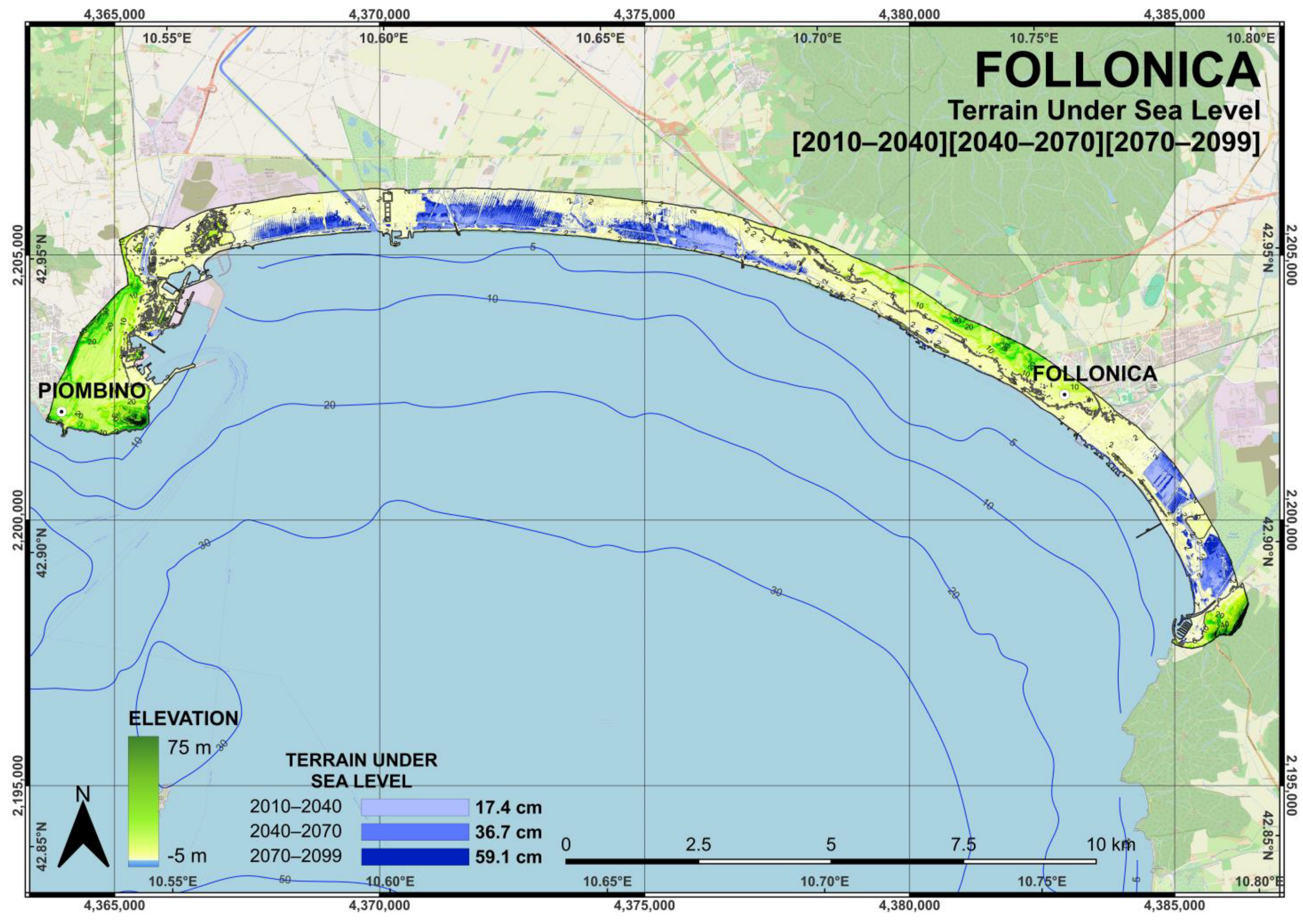
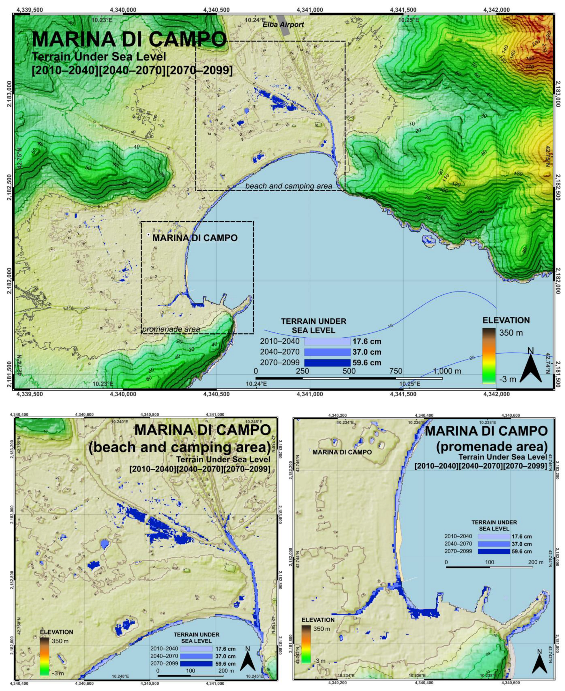
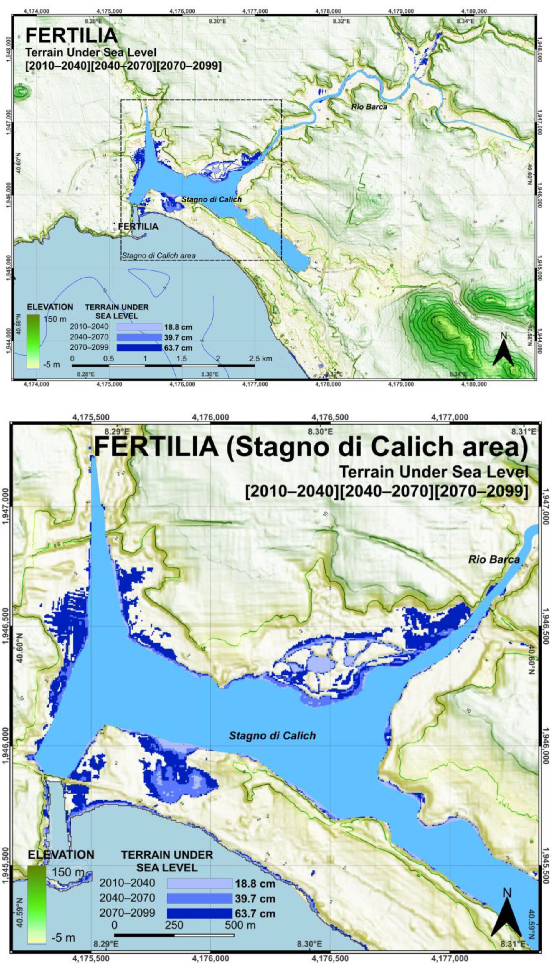
| RSLR (cm) | 21.44 | 44.86 | 71.22 | 23.5 | 48.73 | 76.84 | 22.39 | 46.91 | 74.42 |
| SULS (km2) | 1.36 | 2.72 | 4.57 | 0.04 | 0.06 | 0.09 | 0.99 | 1.13 | 1.44 |
| Study Area | Rome | Latina-Sabaudia | |||||||
| Year | 2040 | 2070 | 2099 | 2040 | 2070 | 2099 | |||
| RSLR (cm) | 23.62 | 48.87 | 76.98 | 25.05 | 51.62 | 81.26 | |||
| SULS (km2) | 1.99 | 3.31 | 5.84 | 9.43 | 12.05 | 14.84 | |||
| Piombino-Follonica | Marina di Campo | Alghero-Fertilia | ||||||||||
| Terrain Under Sea Level | 2010 | 2040 | 2070 | 2099 | 2010 | 2040 | 2070 | 2099 | 2010 | 2040 | 2070 | 2099 |
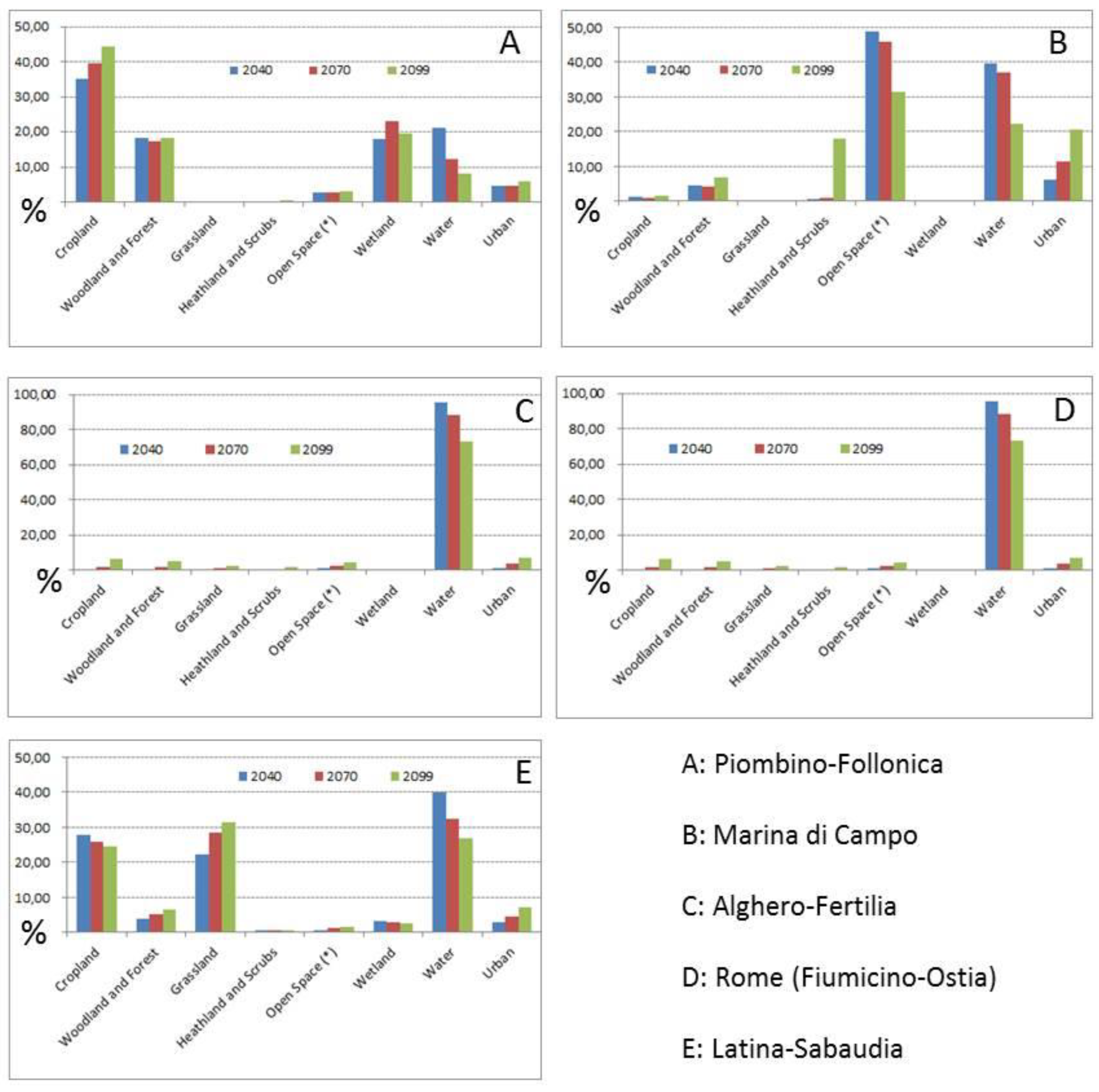
| Cropland | 26.60 | 35.20 | 39.60 | 44.60 | 1.54 | 1.03 | 0.96 | 1.52 | 2.83 | 0.68 | 1.92 | 6.36 |
| Woodland and Forest | 12.30 | 18.30 | 17.30 | 18.30 | 1.54 | 4.38 | 4.19 | 6.69 | 0.53 | 0.45 | 1.52 | 5.37 |
| Grassland | 0.00 | 0.01 | 0.05 | 0.10 | - | - | - | - | 2.49 | 0.59 | 0.98 | 2.39 |
| Heathland and Scrubs | 0.01 | 0.03 | 0.30 | 0.46 | 0.14 | 0.21 | 0.88 | 17.90 | - | 0.12 | 0.52 | 1.49 |
| Open Space 1 | 2.98 | 2.64 | 2.74 | 3.11 | 43.40 | 48.80 | 45.70 | 31.20 | 11.60 | 1.40 | 2.57 | 4.07 |
| Wetland | 17.60 | 18.00 | 23.00 | 19.50 | - | - | - | - | - | - | - | - |
| Water | 35.30 | 21.20 | 12.40 | 8.15 | 45.90 | 39.60 | 36.90 | 22.00 | 68.80 | 95.40 | 88.50 | 73.30 |
| Urban | 5.19 | 4.57 | 4.55 | 5.83 | 7.55 | 6.03 | 11.40 | 20.60 | 13.70 | 1.34 | 3.96 | 6.98 |
| Rome | Latina-Sabaudia | |||||||||||
| Terrain Under Sea level | 2010 | 2040 | 2070 | 2099 | 2010 | 2040 | 2070 | 2099 | ||||
| Cropland | 31.70 | 42.70 | 43.20 | 38.60 | 29.30 | 27.80 | 25.80 | 24.50 | ||||
| Woodland and Forest | 12.10 | 8.71 | 6.85 | 7.75 | 2.04 | 3.62 | 5.21 | 6.50 | ||||
| Grassland | 0.13 | 0.24 | 0.96 | 3.07 | 15.30 | 22.30 | 28.40 | 31.20 | ||||
| Heathland and Scrubs | 0.01 | 0.12 | 0.36 | 0.39 | - | 0.00 | 0.00 | 0.00 | ||||
| Open Space 1 | 5.35 | 6.25 | 6.84 | 6.14 | 0.41 | 0.64 | 1.14 | 1.58 | ||||
| Wetland | 2.10 | 3.72 | 5.61 | 5.14 | 3.66 | 3.16 | 2.74 | 2.42 | ||||
| Water | 35.80 | 25.20 | 17.90 | 11.80 | 48.00 | 39.80 | 32.30 | 26.60 | ||||
| Urban | 12.80 | 13.10 | 18.20 | 27.10 | 1.28 | 2.73 | 4.44 | 7.16 | ||||
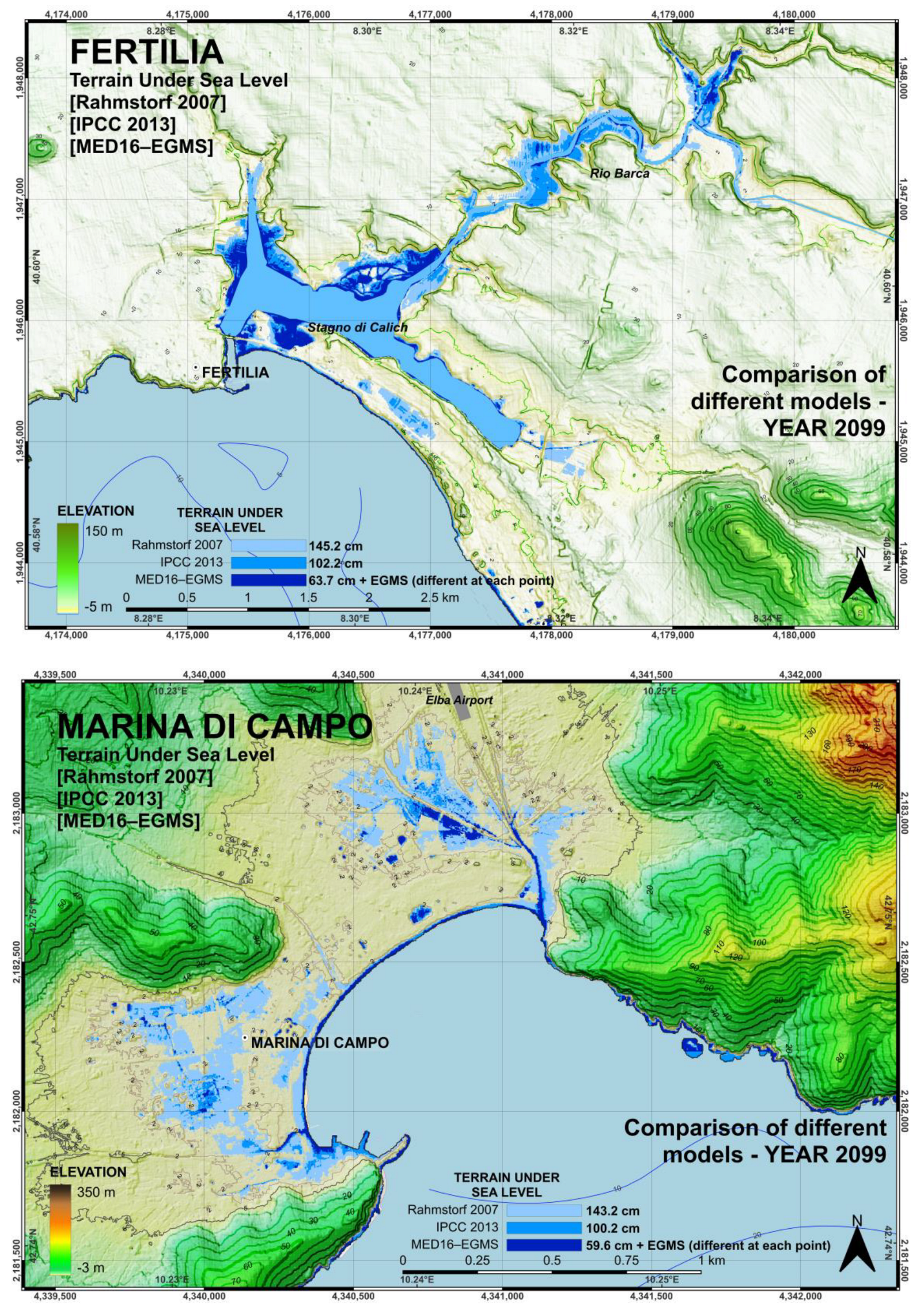
| Marina di Campo | Fertilia | |||
|---|---|---|---|---|
| SLR (cm) | SUSL (km2) | SLR (cm) | SUSL (km2) | |
| Rahmstorf 2007 * | 143.2 | 0.39 | 145.2 | 2.29 |
| IPCC 2013 * | 102.2 | 0.14 | 102.2 | 1.89 |
| MED16 2022 ** | 58.3 | 0.09 | 62.6 | 1.44 |
Disclaimer/Publisher’s Note: The statements, opinions and data contained in all publications are solely those of the individual author(s) and contributor(s) and not of MDPI and/or the editor(s). MDPI and/or the editor(s) disclaim responsibility for any injury to people or property resulting from any ideas, methods, instructions or products referred to in the content. |
© 2024 by the authors. Licensee MDPI, Basel, Switzerland. This article is an open access article distributed under the terms and conditions of the Creative Commons Attribution (CC BY) license (https://creativecommons.org/licenses/by/4.0/).
Share and Cite
Cappucci, S.; Carillo, A.; Iacono, R.; Moretti, L.; Palma, M.; Righini, G.; Antonioli, F.; Sannino, G. Evolution of Coastal Environments under Inundation Scenarios Using an Oceanographic Model and Remote Sensing Data. Remote Sens. 2024, 16, 2599. https://doi.org/10.3390/rs16142599
Cappucci S, Carillo A, Iacono R, Moretti L, Palma M, Righini G, Antonioli F, Sannino G. Evolution of Coastal Environments under Inundation Scenarios Using an Oceanographic Model and Remote Sensing Data. Remote Sensing. 2024; 16(14):2599. https://doi.org/10.3390/rs16142599
Chicago/Turabian StyleCappucci, Sergio, Adriana Carillo, Roberto Iacono, Lorenzo Moretti, Massimiliano Palma, Gaia Righini, Fabrizio Antonioli, and Gianmaria Sannino. 2024. "Evolution of Coastal Environments under Inundation Scenarios Using an Oceanographic Model and Remote Sensing Data" Remote Sensing 16, no. 14: 2599. https://doi.org/10.3390/rs16142599
APA StyleCappucci, S., Carillo, A., Iacono, R., Moretti, L., Palma, M., Righini, G., Antonioli, F., & Sannino, G. (2024). Evolution of Coastal Environments under Inundation Scenarios Using an Oceanographic Model and Remote Sensing Data. Remote Sensing, 16(14), 2599. https://doi.org/10.3390/rs16142599