Abstract
The proliferation of electronic countermeasure (ECM) technology has presented military radar with unprecedented challenges as it remains the primary method of battlefield situational awareness. In this paper, a joint antenna scheduling and power allocation (JASPA) scheme is put forward for multi-target tracking (MTT) in the distributed multiple-input multiple-output (D-MIMO) radar. Aiming at radar resource scheduling in the presence of range deception jamming (RDJ), the false target discriminator is designed based on the Cramer–Rao lower bound (CRLB) in terms of the spoofing range, and the predicted conditional CRLB (PC-CRLB) plays a role in evaluating tracking accuracy. The JASPA scheme integrates the quality of service (QoS) principle to develop an optimization model based on false target discrimination, with the objective of enhancing both the discrimination probability of false targets and the tracking accuracy of real targets concurrently. Since the optimal variables can be separated in constraints, a four-step optimization cycle (FSOC)-based algorithm is developed to solve the multidimensional non-convex problem. Numerical simulation results are provided to illustrate the effectiveness of the proposed JASPA scheme in dealing with MTT in the RDJ environment.
1. Introduction
Under the background of electronic warfare (EW), the working environment of the radar system may be maliciously affected by electronic jammers, thus weakening its combat capability [1]. Generally speaking, when the self-defense jammer interferes with the main lobe of a single-station radar, its anti-interference ability is very limited due to the finite observation angle and single information source [2]. Owing to the “defocused transmit focused receive” (DTFR) working mode, the distributed multiple-input multiple-output (D-MIMO) radar is capable of transmitting wide beams to illuminate the surveillance area and synthesize the focused beams at the receiving end [3], which enhances spatial resolution and brings higher degrees of freedom [4]. Thus, the D-MIMO radar can combine the observation information of multiple channels to expand detection coverage and enhance parameter estimation capability, which shows great potential in the electronic counter-countermeasure (ECCM) [5,6]. However, when the D-MIMO radar performs the MTT task that the tracked targets carry with the self-defense jammer, due to its limited communication capability, the data processing speed of the fusion center, and the total transmit power budget [7,8], anti-jamming performance still needs to be guaranteed by an effective resource scheduling strategy.
In general, aiming at the target tracking scenario, the resource scheduling studies in the D-MIMO radar system consist of two categories, i.e., transmit parameter allocation [9,10,11,12,13,14] and array architecture configuration [15,16,17,18,19,20,21]. As for the transmit parameter allocation problem, ref. [9] studies the single target tracking (STT) scenario in the D-MIMO radar system and constructs the power allocation problem as a cooperative game model. Focusing on the multi-target tracking (MTT) scenario, by introducing the posterior Cramer–Rao lower bound (PCRLB) as an error estimate criterion, ref. [10] proposes a dynamic receive beam allocation algorithm. According to the principle of the low probability of intercept (LPI), in order to achieve the expected estimate accuracy and take into account the communication requirements at the same time, ref. [11] develops a power allocation model by reducing the radar power and the wireless communication power. Since the optimal variables of sensor subset selection, transmit power, and effective bandwidth are coupled in the objective function, ref. [12] designs the sequential parametric convex approximation (SPCA) method to solve the multidimensional joint resource allocation problem. Considering tracking multiple targets in the presence of a hostile interceptor, ref. [13] studies the LPI-based collaborative resource allocation model by reducing the transmit power and effective bandwidth of the transmitted signals under the premise of meeting the given tracking task requirements. In order to enhance tracking performance and maintain anti-interception ability, ref. [14] expands upon the joint transmit beampattern optimization and resource allocation scheme, where the maneuvering target assignment integrated with beampattern optimization and bandwidth allocation are tackled simultaneously.
As for the array architecture configuration problem in the D-MIMO radar system, ref. [15] formulates the joint antenna deployment and power allocation model for enhancing detection performance and proposes a water-filling method to solve the optimization model. Ref. [16] derives the Cramer–Rao lower bound (CRLB) for velocity estimation and proposes an antenna placement algorithm to improve velocity tracking accuracy. By incorporating the transmit antenna position, the receive antenna position, and the allocated transmit power into the Neyman–Pearson (NP) detector, ref. [17] develops collaborative transmit-receive antenna deployment integrated with a transmit power allocation strategy. An efficient node selection and power allocation algorithm in a radar network is proposed by [18], which can enhance the worst-case tracking accuracy in the MTT task. Aiming at the MTT scenario in the clutter environment using the large-scale D-MIMO radar network, ref. [19] proposes the subarray selection and power allocation algorithm with the optimization direction of improving the overall tracking accuracy. The authors of ref. [20] realize the online antenna scheduling of radar networks by dwell time allocation and establish a general framework with respect to self-adaptive radar resource allocation. In order to further improve the LPI capability of the D-MIMO radar system, by minimizing the interception probability of transmit signals when meeting tracking accuracy requirements, ref. [21] constructs an optimization model based on transmit node selection and the transmit power allocation.
Although the existing research on radar resource scheduling provides some useful guidance for solving the MTT problem under non-ideal detection conditions, the electronic interference scenario is rarely involved. In modern EW, jamming equipment can actively transmit or retransmit electromagnetic waves, seriously affecting radar detection, tracking, and recognition, which is called active jamming. According to the different effects, radar active jamming can be divided into active blanket jamming and active deception jamming. Active blanket jamming reduces the signal-to-noise ratio (SNR) of echoes by transmitting high-energy noise or noise-like signals [22], thus reducing detection probability and estimation accuracy. Active deception jamming means that the jammer generates false target information by intercepting, modulating, and forwarding radar signals to cover the real target [23]. In summary, the existing radar anti-jamming methods can be roughly divided into three categories: (1) Reducing the interception probability. By controlling transmit power and developing parameter agility to reduce the interception probability of the radar system [24,25], the estimation of radar parameters by reconnaissance equipment can be affected. (2) Avoiding jamming signal processing. By using sidelobe cancellation, sidelobe blanking, and waveform diversity methods [26,27], the jamming signals are suppressed at the radar receiving end to prevent them from entering the signal processing equipment. (3) Suppressing the mainlobe jamming signal by signal processing. When the jamming signals enter the signal processing equipment through the mainlobe, mainlobe jamming is suppressed by signal processing methods, e.g., multi-domain filtering, subspace separation, and jamming reconstruction cancellation [28,29]. It can be seen that the research on existing anti-jamming technology focuses on different periods, i.e., before, during, and after the entry of jamming signals, but most of the research focuses on the suppression of active blanket jamming and the discussion of countering active deception jamming is not sufficient. Moreover, many existing anti-jamming technologies based on signal processing often cause the loss of the real target signal while suppressing interference.
Many studies in the literature have proved that using radar resource management technology to suppress blanket jamming from the perspective of data processing has obvious effects and broad application prospects [1,3,9,13,14,21,22,24]. In this case, it is also of great research value to use the spatial diversity gain of the D-MIMO radar to counter range deception jamming by reasonably scheduling radar system resources. However, due to the lack of studies on radar resource scheduling in the context of deception jamming, when faced with a complex electromagnetic environment and diversified task scenarios, the previous radar resource scheduling strategies are unlikely to work effectively and are likely to cause task scheduling failures. For instance, if an enemy target carries a self-defense jamming pod or is covered by an electronic jammer escort, more flexible scheduling schemes are needed to improve the signal-to-noise and jamming ratio (SNJR) or implement false target identification. However, as far as our information goes, radar resource scheduling under deception jamming for MTT applications has not been effectively developed before. Due to the possibility that range deception jamming can be identified by the multi-station radar system on the spatial resolution cell, in order to apply this property to the multi-target tracking scenario, this paper pertinently studies the dynamic selection problem of the transmit antenna and receive antenna based on the distributed MIMO radar. In this case, if the optimal tracking channels can be dynamically selected according to the characteristics of range deception jamming and the relative position relationship between the target and the radar antenna, the capability of radar with respect to identifying false targets can be theoretically increased. In addition, there is a coupling relationship between transmit power allocation and transmit antenna scheduling in the D-MIMO radar system, and the joint optimization of the two resources can further improve resource utilization. Therefore, this paper focuses on the MTT task by utilizing the D-MIMO radar and examines the joint antenna scheduling and power allocation (JASPA) scheme under range deception jamming (RDJ). The primary works and contributions are outlined as follows.
(1) The discriminating algorithm for false targets based on the CRLB is developed and the parallel modified particle filter (MPF) is built to judge false targets in real-time and pertinently perform tracking tasks. By deriving the CRLB of the range spoofing parameter and combining the statistical principle, the false target discriminator is established as a hypothesis test on the chi-square distribution. In order to reduce the influence of RDJ on the filtering algorithm, the particle filter (PF) is modified according to the characteristics of the RDJ scenario, and the discrimination probability of false targets is coupled with the MPF to ensure that reliable parameter estimation results can be obtained steadily.
(2) A collaborative resource management approach is suggested for MTT based on the D-MIMO radar while dealing with the RDJ implemented by the self-defense jammer. For a precise description of tracking accuracy, the predicted conditional CRLB (PC-CRLB) of the time delay and the Doppler frequency are jointly calculated and applied to formulate an objective function. Due to the fact that false targets can waste considerable radar resources in practice, an effective JASPA scheme is proposed to address this issue. According to the computed discrimination probability of false targets, the JASPA model is formulated by enhancing the sum of tracking utility values corresponding to the identified true target under the predetermined system resource. In this case, the D-MIMO radar can improve the identification ability of false targets while maintaining the quality of service (QoS) for performing tracking tasks, and finally enhance radar anti-interference capability.
(3) In order to efficiently obtain the suboptimal solutions of the formulated non-convex and NP-hard problem, a four-step optimization cycle (FSOC)-based algorithm is developed. As the Boolean variables of transmit–receive antenna scheduling, the continuous power allocation variable, and the indicator value are coupled in an objective function and constraints, the JASPA model is a discontinuous non-convex and NP-hard problem. To improve solving efficiency and ensure solution accuracy, the step-by-step approach and the smoothing technique are adopted to relax the original problem, and the proximal alternating direction method of multipliers (P-ADMM) algorithm is repeatedly applied to solve the relaxed models. Finally, in order to reduce the system error introduced by relaxation operation, the cyclic minimization technique is adopted to control the solution accuracy.
The subsequent sections of this paper are structured as follows. Section 2 presents the system model, and Section 3 provides the tracking filter in detail and derives the PC-CRLB of the time delay and the Doppler frequency. Section 4 formulates the JASPA model and develops an iterative four-step solution technique to solve the proposed optimization model. Section 5 illustrates the detailed numerical simulation results to verify the effectiveness of the proposed JASPA scheme. Lastly, conclusions are summarized in Section 6.
2. System Model
Consider a D-MIMO radar with M transmitters and N receivers that are dispersedly deployed in the two-dimensional space, where the set of transmitters and the set of receivers are denoted as and , respectively. Moreover, suppose transmitter m and receiver n are separately situated at distinct locations and , where and . For briefness, we give the following assumptions:
(a) The D-MIMO radar system operates in the DTFR mode and continuously undertakes target tracking tasks in the region of interest (ROI).
(b) The ROI consists of Q point-like targets, and all targets are widely separated and maintain the cruising state. For the D-MIMO radar system, the number of moving targets in the ROI is known as a priori information before tracking them in the RDJ environment.
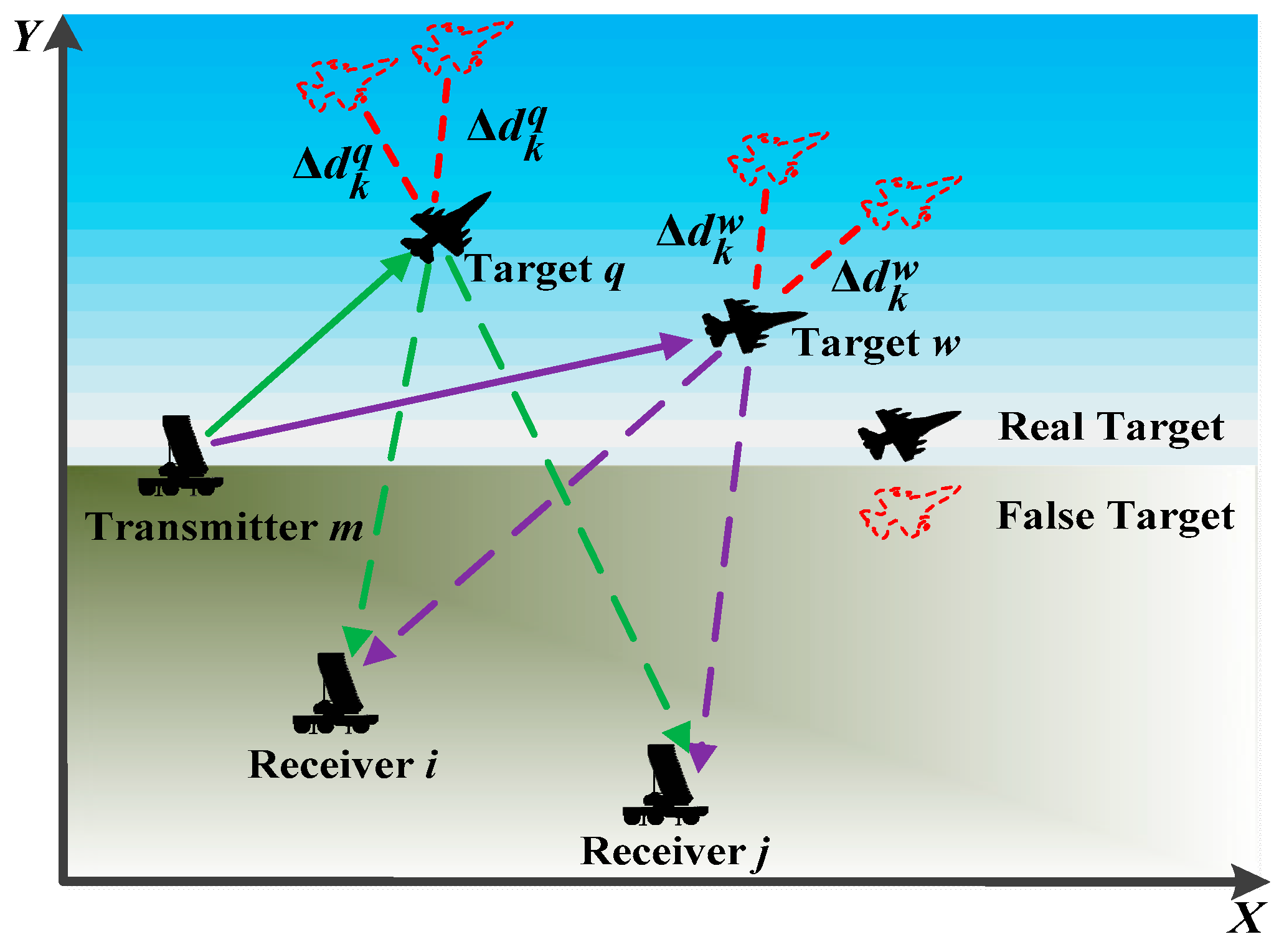
(c) In order to protect real targets from being attacked, the airborne self-defense jammers implement deception jamming by continuously delaying and retransmitting transmit signals from all air defense radars.
(d) Although the deception jammer is able to generate different false targets in theory, herein, we assume that each jammer only generates one false target for each tracking radar at the same time.
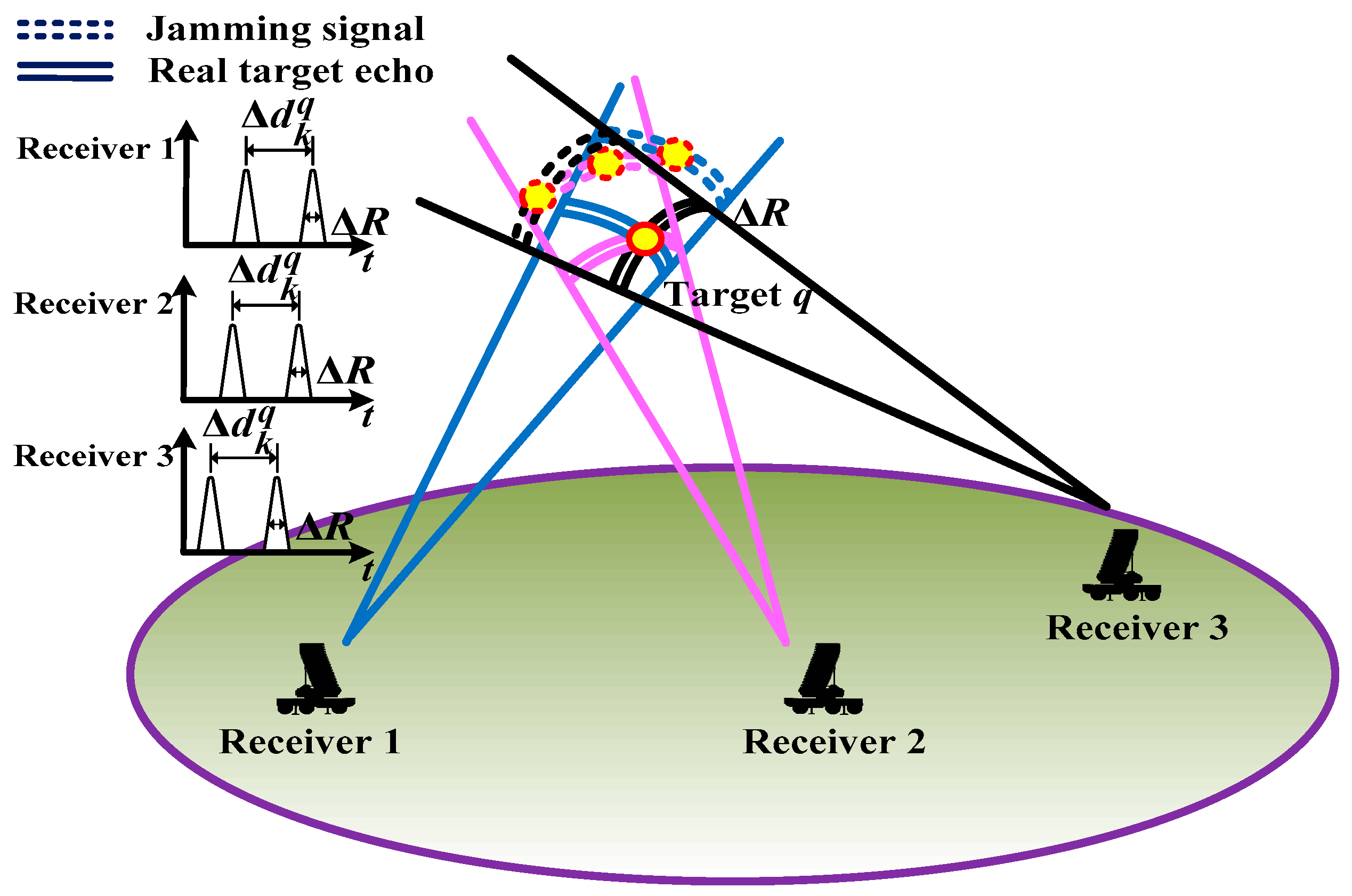
The MTT process in the RDJ environment can be intuitively demonstrated, as shown in Figure 1.

Figure 1.
Illustration of the MTT tracking scheme in the presence of RDJ.
2.1. Signal Model
Assume that all the transmitted signals are narrowband and orthogonal. In this case, we can normalize the transmitted signal from the mth transmitter as
Moreover, the bandwidth and the time width of transmitted signal can be given by
where denotes the equivalent form of after the Fourier transformation.
In the path, the baseband signal reflected by target q at sample interval k is
where represents the attenuation of signal strength due to the bistatic path loss effect, satisfying [15]
where denotes the transmit power from transmitter m, represents the distance between transmitter m and target q, and indicates the distance between receiver n and target q, given by
where represents the location of the qth target. Herein, is the radar cross-section (RCS) of the qth target, which is modeled as a complex parameter and satisfies . The term of represents the combination of the time delay from the real target and active deception jamming, which can be calculated as
where denotes the spoofing distance parameter imposed by the airborne jamming system carried by target q, and c represents the speed of light. In theory, the real radial distance is obtained when , and the false target can be generated when . In this case, the spatial resolution cells (SRCs) of jamming signals and real echoes may become spatially intertwined for a given target, which can be intuitively shown as in Figure 2. Herein, represents the Doppler frequency which is expressed as [16]
where denotes the signal wavelength, represents the azimuth angle of target q to transmitter m, and indicates the azimuth angle of target q to receiver n, respectively.
where represents the four-quadrant inverse tangent operation. Herein, the term of denotes the complex Gaussian noise.
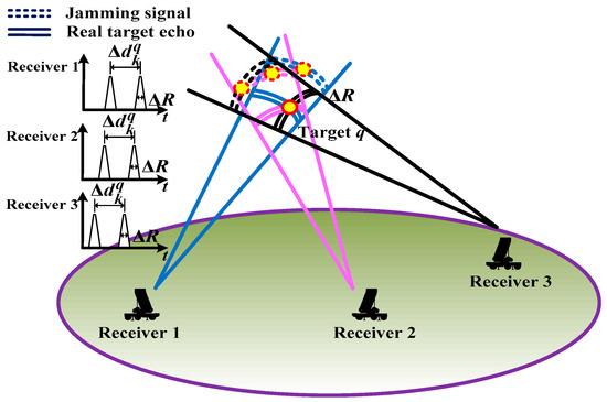
Figure 2.
Diagram of the mixed SRCs under the RDJ scenario.
2.2. Motion Model
For simplicity, consider that all the moving targets satisfy the nearly constant velocity (NCV) model [30]
where is the moving state of target q at sample interval k, and F is the state transition matrix, given by
where denotes the sample interval, represents the second-order identity matrix, and the term of denotes the Kronecker productor. Herein, represents the process noise, and the covariance matrix is computed by
where denotes the noise intensity during the state transition process [31].
2.3. Measurement Model
Using the maximum likelihood (ML) estimation algorithm [32] allows for extracting valuable information from the received signal as outlined in (4), such as the time delay and the Doppler frequency, while the relevant process is shown in Appendix A. We define two binary vectors for selecting transmitters and receivers at the kth sample interval
where , , for and . With the combination of the binary antenna selection variables, the relevant measurement model can be denoted by
Herein, denotes the nonlinear transform function with . According to (7), it is essential to state that the measured data are derived from the real target when , otherwise, they are from false targets. represents the zero-mean Gaussian noise, and the corresponding covariance matrix . Herein, is the CRLB in terms of the time delay and Doppler frequency, which are derived in the next subsection. For future use, we defined the measured dataset of target q from different channels as
2.4. Identification Model
In practice, the range spoofing parameter serves as a valuable tool for distinguishing between real targets and false targets in the RDJ scenario [5]. Mathematically, due to the presence of estimation error, the estimated outcome of variable can be considered as a stochastic process, which satisfies . Herein, the term of denotes the CRLB on the range spoofing parameter, which is given in Appendix B.
Based on the NP detection theory [33], we utilize as the statistical discriminator, and two hypotheses are given by
where represents that , thus the qth target is discriminated as genuine. Conversely, denotes that , so the identification of a false target is declared. The term of represents the chi-square distribution with one degree of freedom, while denotes the noncentral chi-square distribution with one degree of freedom. Given the expected probability for recognizing the real target, denoted as , the identification threshold of the statistical discriminator is given by
where represents the inverse cumulative distribution function of . Therefore, the theoretical discrimination probability of a false target is
where is the theoretical discrimination probability of .
3. Tracking the Filtering Algorithm and Performance Metrics
As shown in Section 2, the measurement data are nonlinear and may contain range drag interference. For the purpose of effectively obtaining the target estimation state in the MTT scenario, in this section, we first outline a parallel MPF which is designed for dealing with the RDJ condition. Moreover, since the PC-CRLB can be calculated in closed form and effectively utilize the actual measurement data, it is employed as an estimation performance metric to guide radar resource scheduling.
3.1. Parallel Modified Particle Filter
The PF surpasses the constraints of the Kalman filter (KF) and is suitable for parameter estimation, especially in situations involving nonlinearity and non-Gaussian noise [34,35]. To prevent particle degradation and suppress the measurement disturbance caused by jamming signals, square-root cubature Kalman filtering (SCKF) [36] and adaptive robust filtering (ARF) [37] are combined with the PF; thus, the MPF can be obtained. In this case, the SCKF is used to assist in selecting importance functions, and the ARF is utilized to reduce the influence of measurement disturbance.
Moreover, the radar system is capable of detecting false targets when the airborne jammers delay and retransmit radar signals through specialized modulation [38]. This case arises due to the possibility of deception jamming signals surpassing the test threshold in the process of target detection [39]. Therefore, we introduced a jamming determination section in the MPF framework. Assume that ς is a given threshold value, and if at the current time, the current measurement information is judged as normal data; otherwise, it would be judged as interference data. Then, the normal data will be substituted into the calculation process to obtain the current time target estimation state, while the interference data will not be sent into the calculation process and the predicted values of the last time will be used as the estimation results at the current time.
With the measurement information , the parallel MPF can be described as follows.
- FOR .
- Initializing the random samples. Let , and assume the initial PDF , , where PN denotes the particle number. Consider that each particle has the same weight .
- Updating the particle state and the covariance matrix by the SCKF algorithm. By introducing and into the SCKF algorithm, the predicted and the predicted are solved. Upon incorporation of measurement data , the updated covariance matrix can be obtained (further information regarding the SCKF algorithm can be found in our previous work [40]). Moreover, the residual of each particle is computed by
- Calculating the adaptive factor. The discriminant statistic of model error can be expressed asand the adaptive factor iswhere is an empirical constant, which is often set as . The term of denotes a constant which is subject to adjustment based on the simulation outcomes.
- Particle set update and particle weight calculation. Incorporating the aforementioned parameters into the SCKF algorithm for the purpose of updating and , the particle state is calculated aswhereMoreover, the particle weight can be expressed by
- IF .
Normalizing the particle weight and resampling the particle set. Let the particle weight be . Then, the new particle sets can be obtained by resampling the particles in according to the corresponding importance weight, and is redistributed. Then, the target state and the relevant variance matrix is updated as
- ELSE.
Let and
Then goes to the recursion step.
- END IF.
- Recursion. Let , and return to the third step.
- END FOR.
3.2. Derivation of PC-CRLB
The CRLB provides a rigorous lower bound for unbiased estimators and may closely approximate the ideal state estimate at the high SNR condition [41]. Since the PC-CRLB is conditioned on the measurement data [42], it is adopted as the performance criterion to fully utilize the measured data with potential instability in RDJ, given by
where denotes the predicted conditional fisher information matrix (PC-FIM), whose inverse is the PC-CRLB matrix. The PC-FIM is computed as [43]
where is the joint probability density function (JPDF), and denotes the operator for the second-order partial derivative with respect to . The PC-FIM is given by [44]
where denotes the prior information, and represents the data information. Mathematically, is defined as
and can be expressed as
In (31), is the Jacobian matrix, where , given by
Herein, let , thus is the FIM with respect to , given by
However, due to the existence of a nonlinear operation, e.g., mathematical expectation, it is difficult to derive an analytical solution of (30) and (31). In the PF framework, the approximation of and can be calculated as [18,19,44]
where and are the estimate matrices of and with respect to . Herein, is the predicted state of without the process noise.
4. JASPA Model Formulation and Solution Strategy
It can be seen from the previous derivation processes that the JASPA results are closely tied to real target tracking accuracy and false target discrimination performance. In practice, due to the limitation of communication on the signal bandwidth and to meet the low interception requirements, the resources available for the distributed radar system are limited [45]. Hence, we formulated a JASPA model to improve anti-jamming ability while ensuring a certain tracking accuracy, and a four-step solving algorithm is proposed subsequently to solve it.
4.1. Problem Formulation
Mathematically speaking, in this paper, the proposed JASPA denotes the non-convex optimization problem which aims at enhancing the anti-jamming capabilities of the D-MIMO radar system. To be specific, the objective function aims at improving both the discrimination probability with respect to false targets and the tracking accuracy with respect to real targets. Inspired by [46], we constructed a two-stage discriminant function to measure whether the discrimination performance of false targets satisfies system requirements. Moreover, in order to better satisfy the requirements of tracking accuracy, the QoS model [47] is introduced to ensure estimate accuracy for all tracked targets in a differentiated manner. In this case, the mathematical representation of the JASPA model at the kth sample interval is
where denotes the threshold of discrimination probability, and the indicator function satisfies
Herein, denotes the task utility value for tracking the qth target, given by
where is the normalization matrix, and represents the expected tracking accuracy.
As for the constraints in (36), constraint indicates that the total number of active antennas is restricted by data processing ability and communication capacity, and denotes the total number of antennas that can be scheduled for performing tracking tasks simultaneously. Constraints and are utilized to keep the D-MIMO radar system in effective operation. To be specific, let the bounds for the antenna scheduling problem be , , , and . Constraints and describe the selection results of the mth transmit antenna and the nth receive antenna by the D-MIMO radar system at sample interval k. Constraint demonstrates that the total power budget is limited and predetermined in practice. Constraint constructs the relationship between transmit antenna selection and power allocation and maintains the normal operation of the radar system while satisfying absolute detection.
Remark 1.
The discrimination probability of the qth target in optimization model is predicted based on a one-step state prediction vector . In addition, it is obvious that the larger spoofing distance and the smaller estimation error will increase the discrimination probability for false targets. Herein, the estimation error is related to the SNR and the spatial relationship between the multi-station radar system and the self-defense jammer, which enables the D-MIMO radar to increase the capability of RDJ resistance by properly dealing with the JASPA problem.
Remark 2.
Since we primarily address the radar resource allocation problem, the parameters in optimization model are assumed to have been initialized and confirmed as a priori knowledge. In addition, for simplicity, it is assumed that the application of RDJ by each target remains consistent throughout the entire tracking process. In this case, the proposed JASPA model can be directly applied from sample interval k = 1. In particular, the threshold of discrimination probability and the expected tracking accuracy can be set from the prior judgment of whether the RDJ is performed by target q.
Remark 3.
By combining the indicator function and the utility value of tracking task , the radar system can perform tracking for the targets that are smaller than the thresholds of discrimination probability, and abandon the targets with higher values than the thresholds of discrimination probability. Specifically, since the task utility value , in order to minimize the objective function in optimization model , the radar system tends to increase the discrimination probability for false targets in a certain range to satisfy . Hence, the proposed JASPA model can improve tracking accuracy for real targets and enhance the capability of identifying false targets simultaneously.
4.2. Solution Technique
Since the maximum number of antennas that can be scheduled at every instant is , the feasible number of active antennas at tracking instant k is . In this case, one possible approach to achieving the optimal solution of antenna scheduling is by systematically enumerating the various configurations of active antennas [48]. Hence, the optimization model can be converted into
where , , , and . In addition, the objective function in is given by
Mathematically, due to the existence of the indicator function and binary selection variables, the optimization model is characterized by its non-convexity and discontinuity, rendering it challenging to solve. In addition, contains both discrete variables related to antenna selection and the continuous variable related to power allocation, which is known to be NP-hard [49]. Since the antenna selection variables and the power allocation variable are separable in constraints, this paper proposes a FSOC approach to approximately solve .
Step 1—Model smoothing. Since the sigmoid function can effectively approximate the indicator function [46], the sigmoid function is adopted to relax the original problem. Furthermore, we relax the discrete variables to and to , for and . Hence, is converted into a smooth non-convex optimization.
Step 2—Transmit antenna selection. Assume that the quantity of active transmit antennas is denoted as , with all receive antennas being assigned for receiving target echo signals. Moreover, the power budget is evenly allocated among the active transmit antennas. At this point, the described optimization model can be expressed as
where .
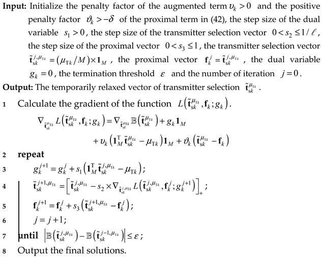
Although the optimization model is greatly relaxed after smoothing and parameter assignment, is still a non-convex problem due to the sigmoid function being non-convex. In order to address the optimization model characterized by a non-convex objective function and linear constraints, the P-ADMM algorithm [50] is adopted to obtain the approximate optimal solution with guaranteed convergence [51]. The fundamental concept underlying the P-ADMM algorithm involves the incorporation of an exponential averaging scheme and the introduction of a proximal term containing the quadratic form to ensure that the non-convex problem, under linear constraints, converges to a steady-state point [50]. To be specific, the augmented Lagrangian function in is computed by
where is the proximal vector, denotes the dual variable, represents the penalty factor of the augmented term, is the positive penalty factor for the proximal term, and is the 2-norm operator. In order to solve , the procedural steps of the P-ADMM algorithm are outlined in Algorithm 1, according to which we can obtain the temporarily relaxed selection vector with respect to transmit antenna . In Algorithm 1, for convergence consideration, we set two constants and to make the two inequalities hold
Specifically, since the solution for the relaxed model can be fractional, the temporary transmitter selection vector can be obtained by selecting the largest elements from to be one and setting the remaining elements to zero [52].
Step 3—Receive antenna selection. By setting the scheduling strategy of the transmit antenna to the solution vector in step 2 and the allocation strategy of transmit power to , the relaxed optimization model of receive antenna selection can be expressed as
Similarly, the optimization model is characterized by non-convexity and can be effectively addressed through the utilization of the P-ADMM algorithm. Considering that the solving process is similar to Algorithm 1 (only the optimization parameters need to be changed to the receive antenna selection variables), the detailed process is not discussed here for brevity. After solving , the largest elements in are assigned as ones to formulate the temporary vector .
Step 4—Transmit power allocation. After obtaining the antenna selection results and , the temporary power allocation results can be achieved via the following optimization model
Similar to the first two steps, the power allocation results can be obtained by solving using the P-ADMM algorithm. Meanwhile, the objective function value of will be repetitively recorded and compared with the previously solved objective function value of in step 2. Thus, the cycle will cease until the discrepancy between the outputs of step 2 and step 4 is below the predetermined termination threshold. The final objective function values of all potential solution sets corresponding to and are compared, with the solution set demonstrating the lowest objective function value being designated as the optimal JASPA strategy. The complete proposed solution methodology is summarized in Algorithm 2.
| Algorithm 1. The general steps of the P-ADMM algorithm for solving model (41). |
 |
| Algorithm 2. Summary of the proposed FSOC approach. |
 |
Remark 4.
In Algorithm 1, the term of in step 4 denotes a projection operator which projects a vector into the non-negative quadrant. In the iterative computation process, updating the dual variable in step 3 and the proximal vector in step 5 is relatively simple and imposes little effect on the computational complexity of the P-ADMM algorithm. However, according to step 1, the updating process of the optimal solution set in step 4 is difficult due to the gradient calculation of the highly nonlinear objective function, which mainly determines the computational complexity of the P-ADMM algorithm.
Remark 5.
The computational complexity of the FSOC-based solving approach is primarily influenced by the predetermined termination threshold in Algorithm 2 and the P-ADMM algorithm. Based on [50], the iteration complexity of the P-ADMM algorithm is . In addition, when solving the temporary transmit antenna selection results , the computational complexity of the P-ADMM algorithm in one iteration is , where denotes the dimension of the target state. Similarly, in one iteration, the computational complexity for solving and are and , respectively. Therefore, considering the amount of work brought by the matrix inversion, i.e., , the total computational complexity of the FSOC-based solving approach is denoted by .
Remark 6.
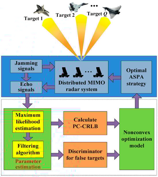
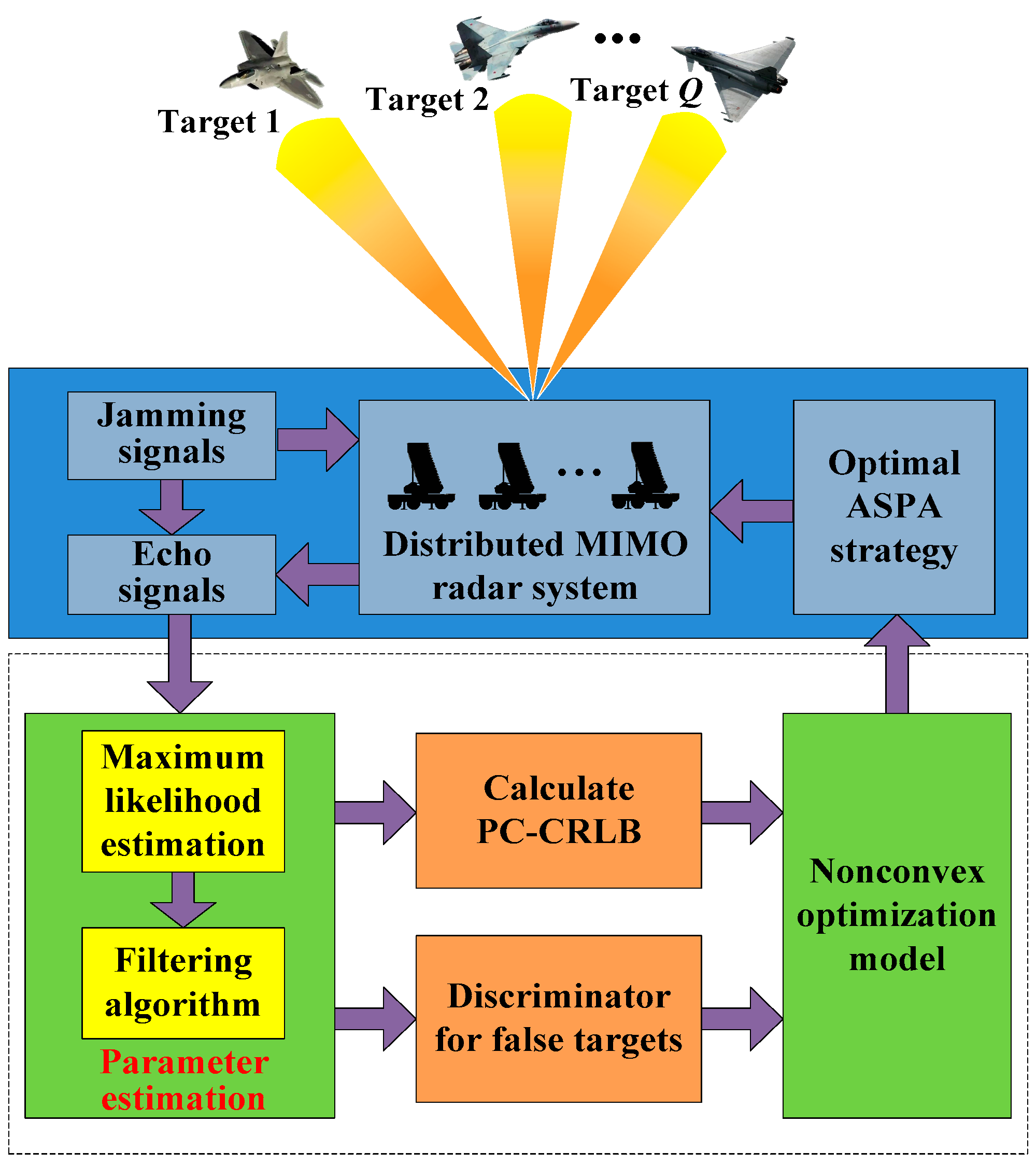
The final solution results are fed back to the radar system to guide the JASPA strategy at the next tracking instant, which leads to a closed-loop tracking framework in the D-MIMO radar [10]. Specifically, by utilizing the PC-CRLB and the constructed discriminator based on the tracking recursive prediction scheme [53], the resource-aware radar system can learn the environment dynamically and formulate a reliable JASPA strategy to improve its anti-jamming capability. Finally, Figure 3 illustrates the flowchart depicting the proposed resource-aware closed-loop tracking process in the D-MIMO radar system.
Figure 3.
Flowchart of the proposed resource-aware tracking framework.
5. Simulation Results
In order to elucidate the efficacy of the formulated JASPA strategy, numerical simulation results are presented in this section. The distributed MIMO radar system with transmit antennas and receive antennas is selected for analysis, where the remaining relevant system parameters are presented in Table 1. Assume that there are targets moving in the ROI, whose initial state is shown in Table 2. In each Monte Carlo trial, 20 frames of data are used for tracking, and the total number of Monte Carlo trials is set as . Moreover, in order to be closer to a real air defense combat environment, it is postulated that a critical defense target is situated at point , and the task of the air defense combat system is to protect the defense target from being attacked. In this case, as for the radar system, the closer the moving target is to the defense target, the lower the expected tracking error should be set. Herein, the task area is divided into three parts by a piecewise function, given by
where denotes the operation of radial distance.

Table 1.
Simulation parameters of the established MTT system in the RDJ environment.
Table 2.
Real initial state of each moving target.
Furthermore, in order to enhance the clarity of parameter estimation performance for each moving target, the normalized PC-CRLB of target q is defined as
where denotes the state estimation result of target q in the jth trial.
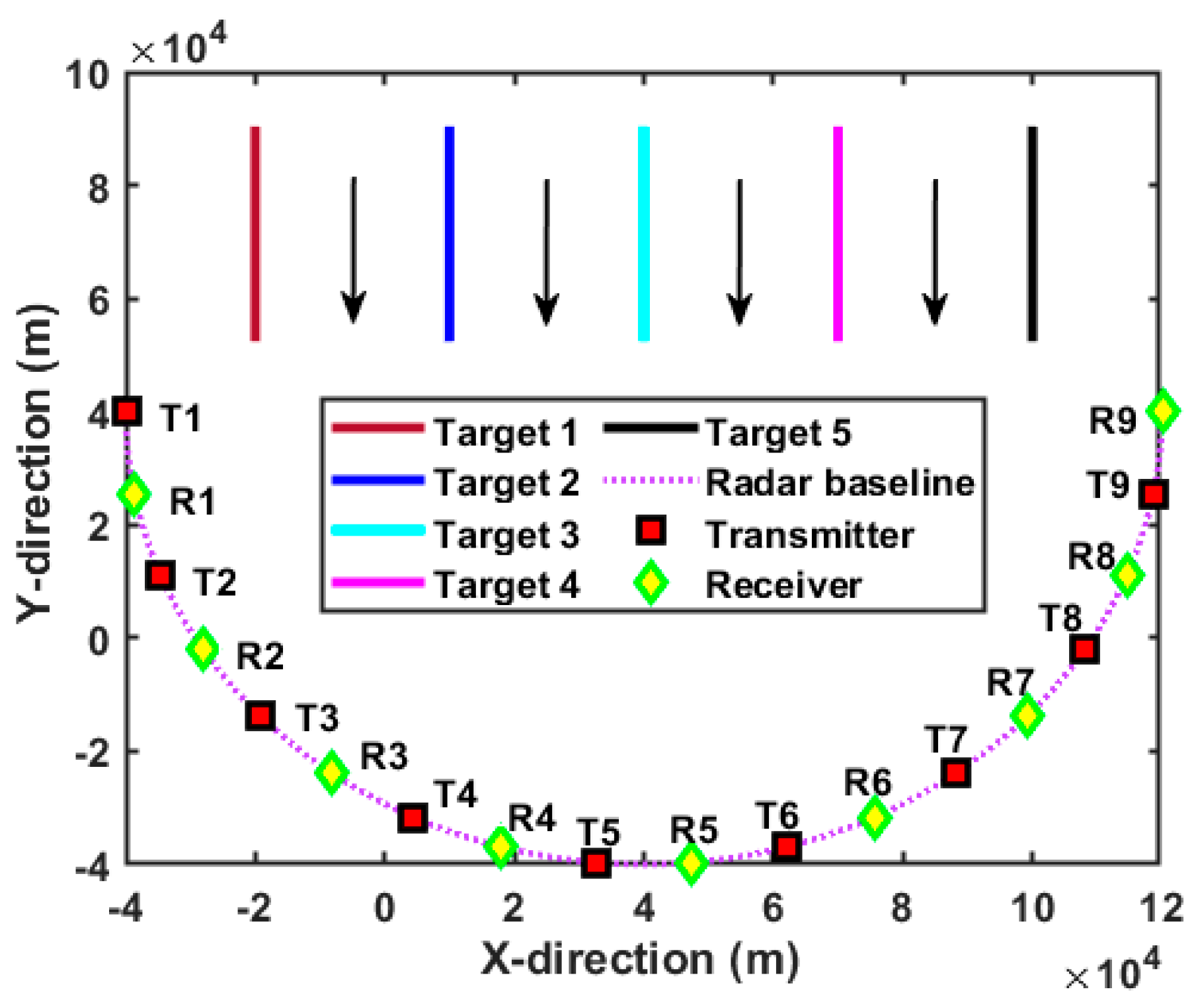
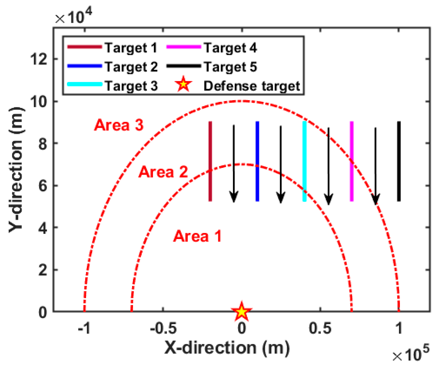
Based on the above simulation condition assumptions, the spatial arrangement of the D-MIMO radar system in relation to the moving targets is illustrated in Figure 4. Specifically, all the transmit antennas and the receive antennas are interspersed, and the formed radar baseline is semicircular. Herein, the red rectangle represents the transmit antenna, and the yellow diamond represents the receiving antenna. In addition, each target moves towards the radar baseline at the same speed, and the distance between adjacent targets is always equal. In order to clearly show the battlefield situation, the geometric relationship of the defense target, the moving targets, and the surveillance areas is intuitively demonstrated in Figure 5. Herein, the pentagram denotes the critical defense target. Based on Equation (47), the surveillance region is divided into three areas displayed by the red dotted line according to the radial distance difference. Apparently, target 5 is always moving in surveillance area 3, while other targets have completed a one-time crossing of the surveillance area. In this case, the radar system has a lower requirement for the tracking accuracy of target 5, and higher requirements for targets that later enter the areas with higher priority, e.g., target 1, target 2, and target 3. It should be emphasized that such a division satisfies the principle of air defense operations, i.e., giving priority to attacking targets with greater threat.

Figure 4.
Target trajectories with respect to the D-MIMO radar system.

Figure 5.
Geometric relationship between the divided surveillance areas and moving targets.
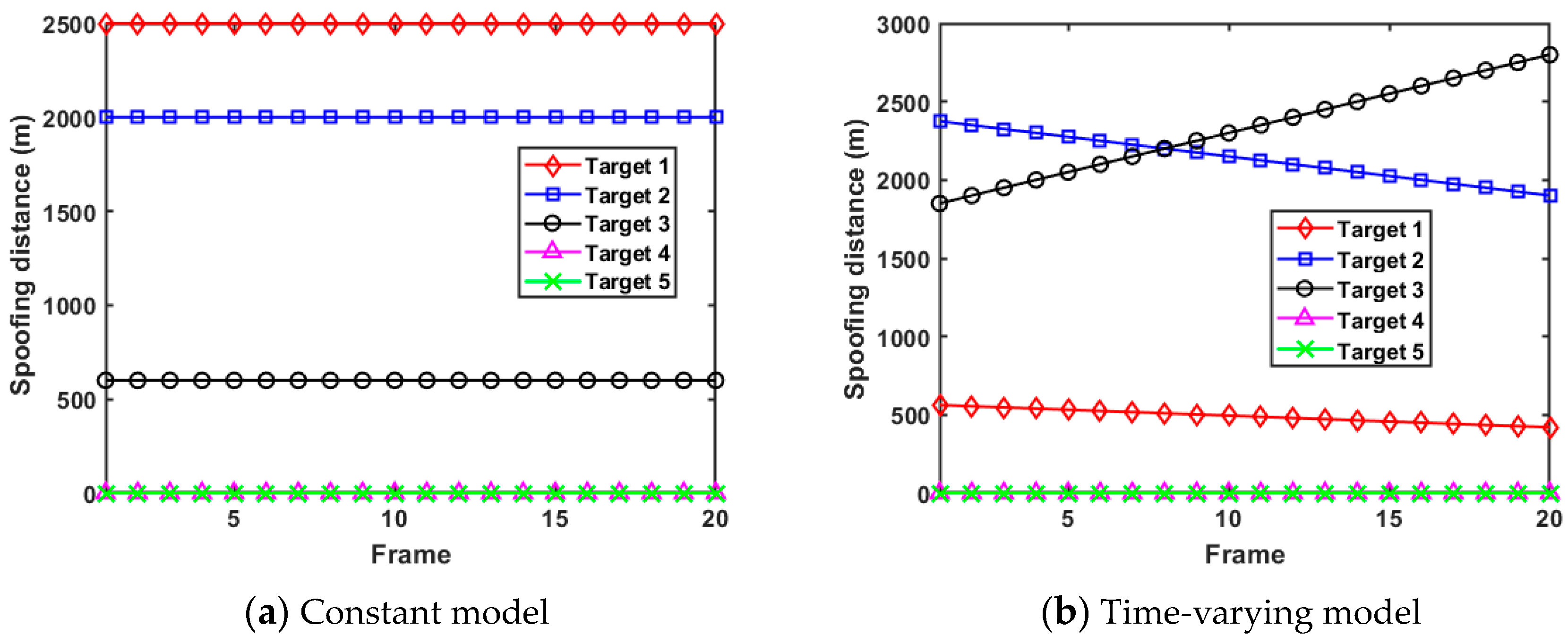
Since the established expected tracking error model is independent of the target RCS, the impact of the RCS on the results of radar resource scheduling should be avoided, so as to better study the RDJ problem. Hence, we assume that the RCSs of all the moving targets are always maintained at 1 m2 for briefness. In order to explore the influence of the spoofing distance parameter on tracking performance and resource scheduling, a constant model and a time-varying model are designed for simulation research, which is demonstrated in Figure 6. It can be seen from Figure 6a that the spoofing distance parameters corresponding to all targets in the constant model are constant with time, and target 1 has the largest setting value of the spoofing distance parameter. Meanwhile, Figure 6b demonstrates that the values of the spoofing distance parameters of target 1, target 2, and target 3 change linearly with time, and the setting values of target 3 increase with time while the setting values of target 1 and target 2 decrease dynamically. It is worth noting that target 4 and target 5 are not supposed to implement jamming in both models, so as to build control experiments with respect to whether to implement the RDJ.
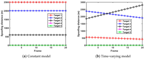
Figure 6.
Two kinds of spoofing distance parameter models.
5.1. Case 1: Constant Spoofing Distance Model
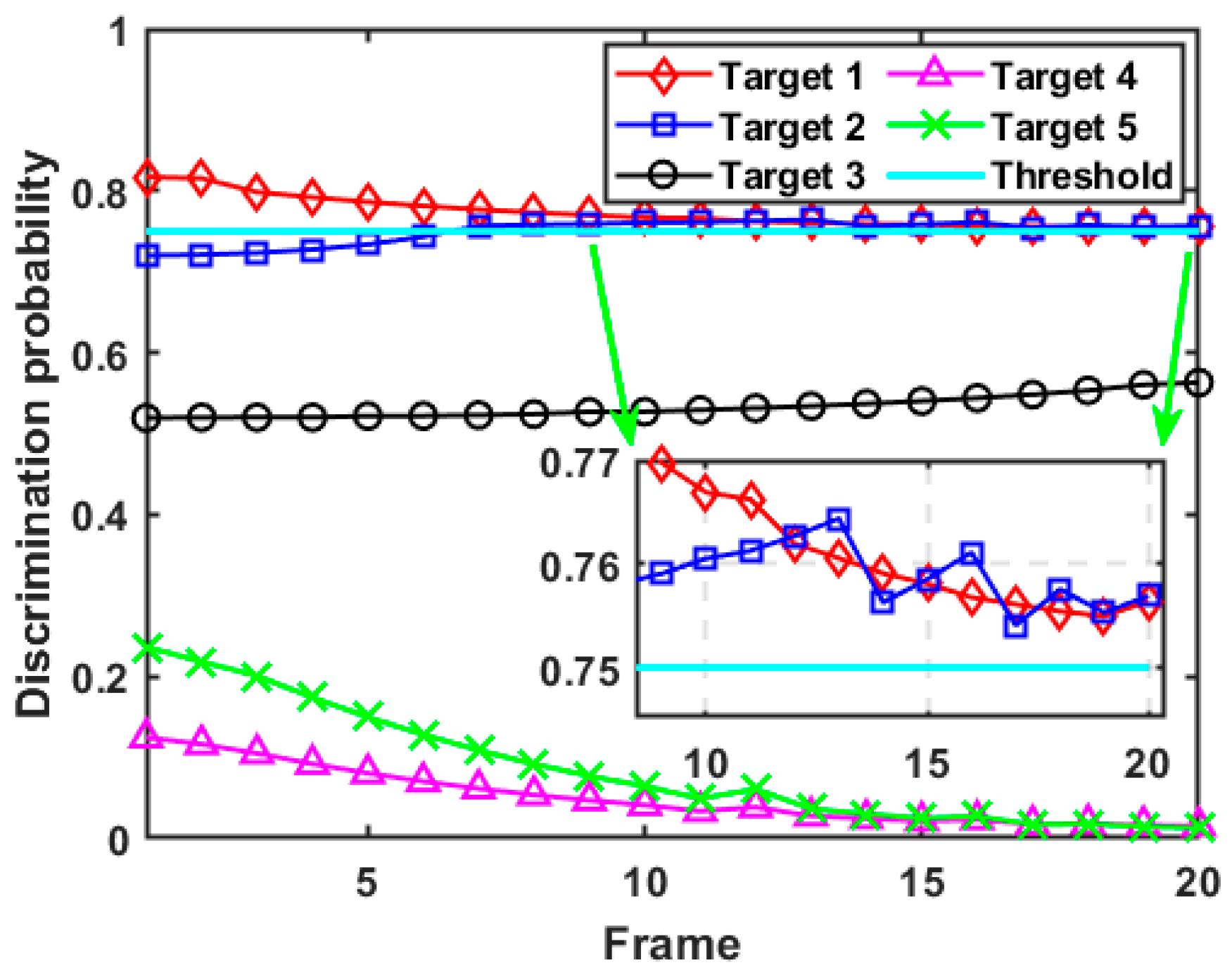
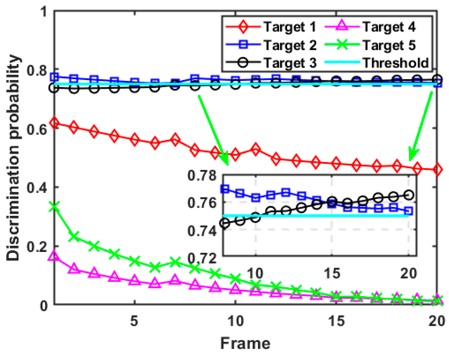
In this case, since the spoofing distance parameters introduced by each target are constant to the D-MIMO radar system, the RDJ strategy carried out by the self-defense jammer does not change with time. The computing results of the discrimination probability for each target in case 1 are given in Figure 7. Due to the implementation of self-defense RDJ, the discrimination probability of target 1, target 2, and target 3 is significantly higher than that of target 4 and target 5. Since target 4 and target 5 do not retransmit radar signals, the calculated discrimination probability from the MIMO radar system is kept at a low level, and gradually decreases with time until it trends to zero. Specifically, after resource optimization scheduling, the discrimination probability of target 1 is always greater than the preset discrimination threshold, so target 1 is identified as a false target throughout the whole tracking process. Meanwhile, although the initial discrimination probability of target 2 is less than the threshold, it starts exceeding the discrimination threshold after the seventh frame. Due to the small spoofing distance parameter of target 3 and the limited resources that the D-MIMO radar system can schedule, the discrimination probability of target 3 increases with time, but it still fails to reach the preset threshold. The discrimination probability of target 4 and target 5 without the RDJ decreases with the increase in tracking accuracy. Moreover, it can be seen from the numerical range of the discrimination probability of each target that the higher the spoofing range parameter setting, the greater the corresponding discrimination probability, which proves the correctness of the formulated discriminator.
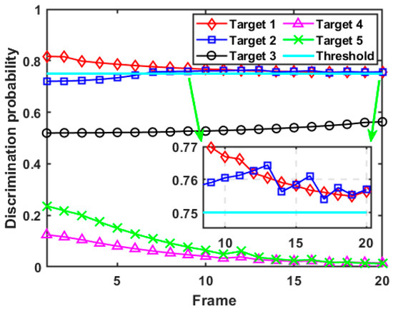
Figure 7.
Discrimination probability of each target in case 1.
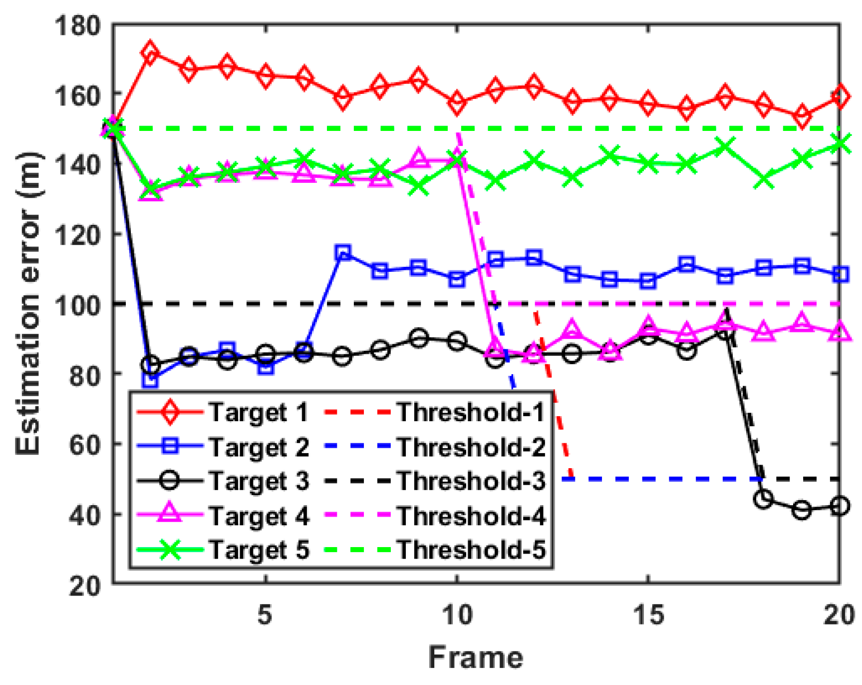
In actual combat, military radar usually does not know the RDJ strategy of the enemy in advance, which may lead to the introduction of biased estimations. Since the PC-CRLB can only provide the lower bound for the unbiased estimation, it is not reliable to judge the tracking performance by analyzing the PC-CRLB of each target without the discrimination results of false targets. In this case, the PC-CRLB and the feasible accuracy threshold of each target are further illustrated in the supplementary data of Figure 7 and Figure 8. It can be seen from Figure 8 that after the identification and screening of false targets, the D-MIMO radar system can achieve a tracking accuracy for real targets that is close to the initial expected tracking accuracy and abandon the strict control of the tracking accuracy of false targets, which leads to stronger adaptive ability.
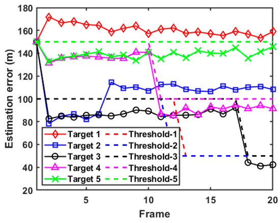
Figure 8.
Estimation error of each target in case 1.
To be specific, combined with Figure 7 and Figure 8, it can be seen that since the D-MIMO radar determines that target 3, target 4, and target 5 are always real targets, the PC-CRLBs of these targets are lower than the thresholds of estimation error after resource scheduling. In addition, due to target 1 being judged as a false target during the whole tracking process, the radar system does not take the tracking performance of target 1 into account, so its PC-CRLB is higher than the corresponding threshold of estimation error. Similarly, target 2 is judged as a false target at the beginning of frame 7, which also causes its PC-CRLB to be higher than the threshold of estimation error after frame 7. On the whole, due to the strong adaptability of the adopted filtering algorithm, the tracking accuracy of each target can be maintained at a relatively low level and always converges, which also reflects the correctness of the established model.
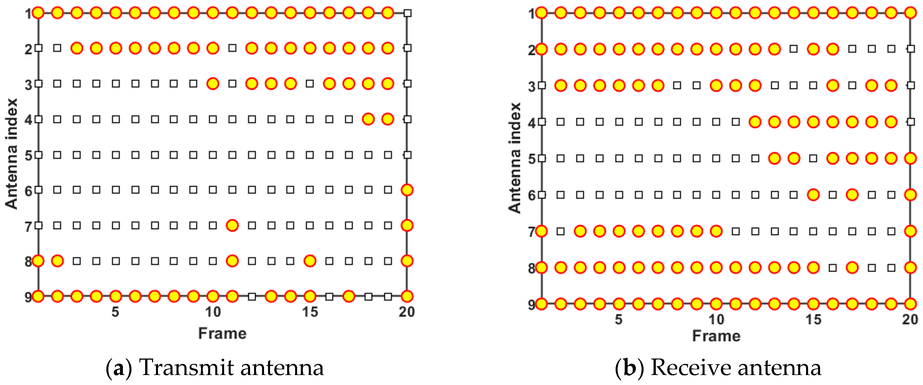
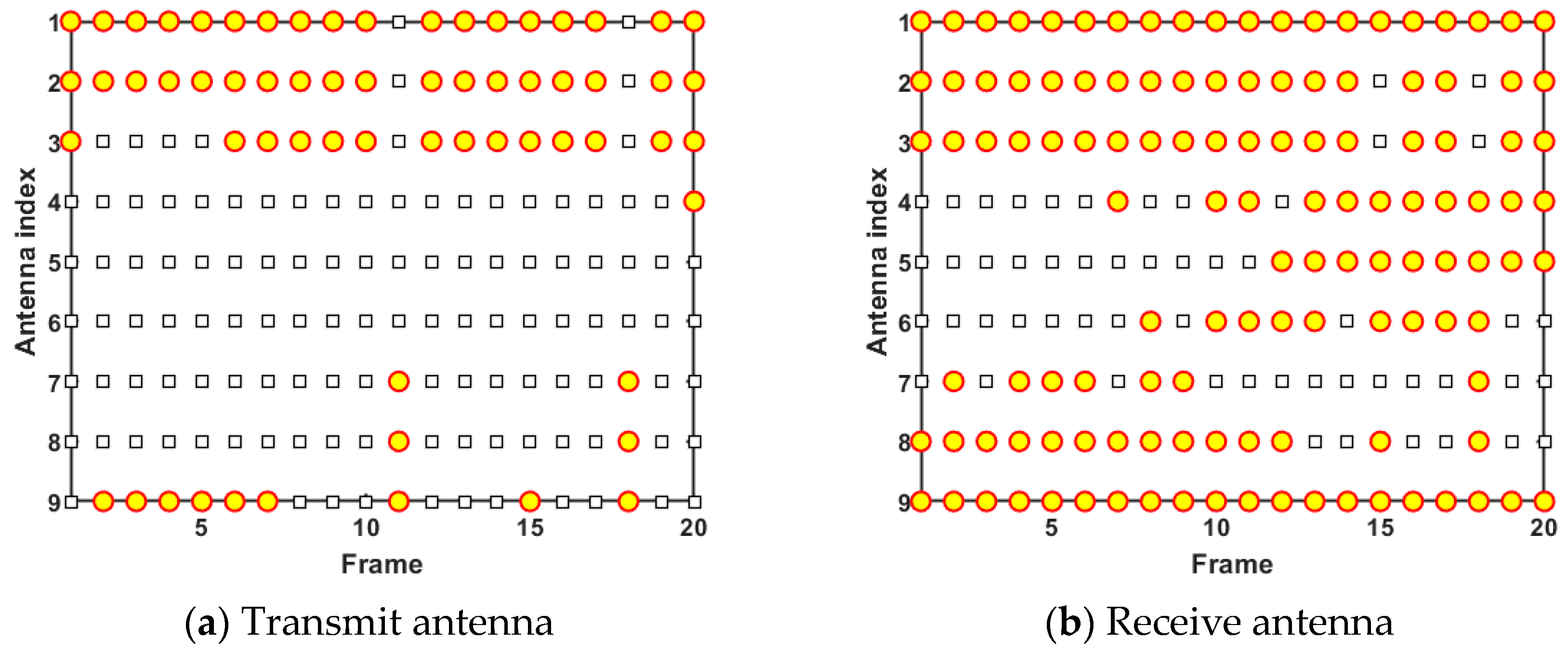
Figure 9 and Figure 10 demonstrate the results of antenna scheduling and power allocation in one simulation trial, respectively. In Figure 9, the yellow circles indicate that the antennas with the corresponding index are active and assigned to perform tracking tasks at the current frame. According to the analysis of Figure 9a, transmit antenna 1, transmit antenna 2, and transmit antenna 9 are scheduled most frequently. The emergence of this phenomenon can be explained by the fact that the three transmit antennas are closer to moving targets and possess better observation positions. In addition, it can be seen from Figure 9b that receive antenna 1, receive antenna 2, receive antenna 8, and receive antenna 9 are scheduled most frequently due to their location advantages. The results shown in Figure 9 demonstrate that although the D-MIMO radar has multiple independent antennas with large distances, the radar system tends to schedule the antennas in dominant positions to participate in the tracking task, so as to maximize the radar performance boundary and improve resource utilization.
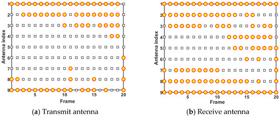
Figure 9.
Antenna scheduling results in case 1.
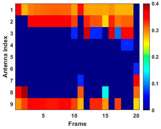
Figure 10.
Transmit power allocation results in case 1.
In Figure 10, the different color in each rectangular box denotes the corresponding transmit power ratio. Herein, the dark blue rectangular box indicates that the transmit power allocation ratio is zero, and the crimson rectangular box represents the highest ratio of transmit power allocation. The results in Figure 10 are consistent with the conclusions in Figure 9a, i.e., transmit antenna 1, transmit antenna 2, and transmit antenna 9 consume most of the transmit power resources in case 1. It can be seen that by jointly optimizing antenna scheduling and transmit power allocation, transmit power resources can be more concentrated to parts of the transmit antennas, and the power quota can be dynamically adjusted according to situational changes.
5.2. Case 2: Time-Varying Spoofing Distance Model
This case investigates the impact of changes in the spoofing distance parameter on tracking performance and resource scheduling over time. As shown in Figure 6b, the spoofing distance parameters of target 1 and target 2 decrease with time, and the initial value of the spoofing distance parameter of target 3 is high and increases rapidly with time. Without loss of generality, the spoofing distance model in case 2 still ensures that the spoofing distance parameters of target 4 and target 5 are consistent with case 1, i.e., always equal to zero.
Figure 11 demonstrates the calculation results of the discrimination probability with respect to each target in case 2. It can be seen from Figure 11 that the variation trend of the discrimination probability for target 1 corresponds roughly to the trend in its spoofing distance parameters, and the results of discrimination probability are always below the preset threshold, suggesting that the radar resource budget is not enough to accurately identify all false targets. In addition, although the spoofing distance parameter of target 2 is always in a decreasing state, due to its large initial value, target 2 is always judged as a false target by the radar system after resource optimal scheduling. The discrimination probability of target 3 increases with the increase of its spoofing distance parameter and exceeds the discrimination threshold after the 11th frame. Similar to case 1, the results of the discrimination probability of target 4 and target 5 always remain at a low level and show a decreasing trend over time, which shows that the discrimination probability for the real target can be reduced with the improvement of its tracking accuracy at the same time. In summary, the calculation results of discrimination probability shown in Figure 11 conform to the change rule of the preset time-varying model of the spoofing distance parameter, which demonstrates the effectiveness and robustness of the formulated discriminator.
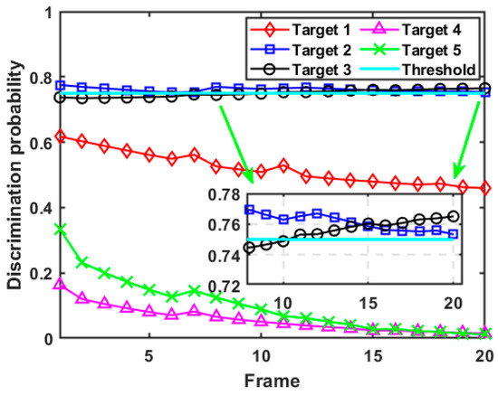
Figure 11.
Discrimination probability of each target in case 2.
The results of estimation error for each target in case 2 are demonstrated in Figure 12. Firstly, combined with Figure 11, it can be seen that since the discrimination probability of target 1, target 4, and target 5 is always lower than the preset discrimination threshold, the radar system regards these three targets as true targets and tracks them according to the expected tracking accuracy. Therefore, the lower bounds of estimation error in terms of target 1, target 4, and target 5 are less than the expected tracking error and can be dynamically adjusted with the target passing through the task area, reflecting higher target tracking accuracy and adaptive ability. In addition, since the discrimination probability of target 2 is higher than its discrimination threshold, target 2 is judged as a false target, so that its PC-CRLB is always unaffected by the expected tracking accuracy. Finally, the discrimination probability of target 3 is always lower than the threshold in the first 10 frames, so its PC-CRLB meets the expected tracking accuracy requirements. However, after the 11th frame, due to the abandonment of the radar system to optimize the tracking performance of target 3, its PC-CRLB shows a significant increase.
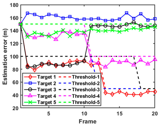
Figure 12.
Estimation error of each target in case 2.
Figure 13 and Figure 14 give the results of antenna scheduling and power allocation in case 2, respectively. According to Figure 13, we can see that the results of antenna scheduling right now are similar to those in case 1, i.e., the radar system tends to assign the antennas closer to moving targets to perform tracking tasks. However, since the intensity of RDJ applied by target 1 is lower than that in case 1, it is difficult for the radar system to accurately identify target 1 as a false target with the finite system resources. In this case, transmit antenna 3 is scheduled more frequently to track target 1, and transmit antenna 9 is less selected for target tracking. It can be seen from Figure 13b that the D-MIMO radar system tends to assign as many receive antennas as possible to measure transmitted signals under the limited number of activable antennas, so as to make full use of the spatial diversity gain to identify false targets.

Figure 13.
Antenna scheduling results in case 2.
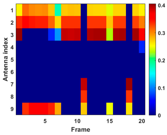
Figure 14.
Transmit power allocation results in case 2.
The results of transmit power allocation shown in Figure 14 are highly consistent with the results of transmit antenna scheduling in Figure 13a, i.e., most transmit resources are allocated to transmit antenna 1, transmit antenna 2, and transmit antenna 3. Specifically, due to the high expected tracking accuracy of target 1, the scheduling frequency and the transmit power of transmit antenna 9 are significantly reduced to meet the tracking performance requirement, while the scheduling frequency and the allocated transmit power of transmit antenna 3 are increased in case 2. In addition, we note that when transmit antenna 3 is assigned to perform tracking tasks, the corresponding ratio of transmit power is usually higher than the ratio in terms of other active transmit antennas, because transmit antenna 3 undertakes the heavy task of effectively improving the tracking accuracy of target 1 to the expected tracking accuracy. In general, from the perspective of resource scheduling results, the proposed algorithm shows good adaptability in dealing with changes in spoofing distance conditions.
6. Conclusions
In this paper, an effective JASPA scheme is developed for the D-MIMO radar system to enhance target tracking performance in the RDJ environment. To enhance the discernment of false targets, based on the characteristics of RDJ, the CRLB-based false target discriminator is built for identifying false targets dynamically, and the PC-CRLB in terms of time delay and the Doppler frequency is derived as the estimation error criterion. On the basis of this, by optimizing the discrimination probability of false targets and the tracking accuracy of real targets, the JASPA model is established to enhance the anti-jamming ability of the D-MIMO radar within the predetermined system resource. Due to the non-convex and NP-hard characteristics of the formulated JASPA model, an FSOC algorithm was developed to relax and solve the original problem. Numerical simulation results show that adopting the JASPA scheme led to improvements in tracking performance and anti-jamming effectiveness.
Author Contributions
Conceptualization, Z.L.; methodology, Z.L. and R.W.; software, Z.L.; validation, Y.Y.; formal analysis, investigation, Z.L.; resources, data curation, Z.L.; writing—original draft preparation, Z.L.; writing—review and editing, C.Q. and J.H.; visualization, Z.L. and C.Q.; supervision, Y.Y.; project administration, R.W.; funding acquisition, R.W. All authors have read and agreed to the published version of the manuscript.
Funding
This work was supported by the Shaanxi Natural Science Foundation Basic Research Project under Grant 2023JCYB509.
Data Availability Statement
The original contributions presented in the study are included in the article, further inquiries can be directed to the corresponding author.
Acknowledgments
The authors would like to thank the Editors and all the reviewers for their very valuable and insightful comments during the revision of this work.
Conflicts of Interest
The authors declare no conflicts of interest.
Appendix A
The process of ML estimation.
At the kth sample interval, we can obtain an observation vector
Based on the received signal model in (4), the conditional PDF satisfies
where . Herein, , , and are expressed as
The ML estimate of can be expressed as
By substituting , the ML estimate of is computed by
Therefore, the target information of the time delay and Doppler frequency of target q at sample interval k is estimated as , which is then put into the filter to update the measurement information.
Appendix B
The derivation of the CRLB for .
According to (4)–(7), the estimate vector of the position parameters is considered as . Hence, the following inequality holds for the unbiased estimate of
where represents the FIM in terms of and can be computed by
We notice that is only related to the delay parameter . Based on the chain rule, we have
Similar with (A7), is defined as
Herein, the term of is derived as
where several geometric relationship parameters are denoted as , , , and .
By substituting (A9) and (A10) into (A8), the CRLB of the estimate vector can be computed by
where is a third-order square matrix, given by
The third element on the diagonal of denotes the CRLB of , which can be expressed as
References
- Li, Z.; Xie, J.; Liu, W.; Zhang, H. Resource optimization strategy in phased array radar network for multiple target tracking when against active oppressive interference. IEEE Syst. J. 2023, 17, 3539–3550. [Google Scholar] [CrossRef]
- Pu, W.; Liang, Z.; Wu, J.; Liu, Q. Joint generalized inner product method for main lobe jamming suppression in distributed array radar. IEEE Trans. Aerosp. Electron. Syst. 2023, 59, 6940–6953. [Google Scholar] [CrossRef]
- Zhang, W.; Shi, C.; Zhou, J. Power minimization-based joint resource allocation algorithm for target localization in noncoherent distributed MIMO radar system. IEEE Syst. J. 2022, 16, 2183–2194. [Google Scholar] [CrossRef]
- Shi, J.; Yang, Z.; Liu, Y. On parameter identifiability of diversity-smoothing-based MIMO radar. IEEE Trans. Aerosp. Electron. Syst. 2022, 58, 1660–1675. [Google Scholar] [CrossRef]
- Zhao, S.; Liu, Z. Deception parameter estimation and discrimination in distributed multiple-radar architectures. IEEE Sens. J. 2017, 17, 6322–6330. [Google Scholar] [CrossRef]
- Zhang, H.; Liu, W.; Zhang, Q.; Liu, B. Joint customer assignment, power allocation, and subchannel allocation in a UAV-based joint radar and communication network. IEEE Internet Things J. 2024, in press. [Google Scholar] [CrossRef]
- Yan, J.; Shi, C.; Dai, J.; Liu, H. Radar sensor network resource allocation for fused target tracking: A brief review. Inf. Fusion 2022, 86, 104–115. [Google Scholar] [CrossRef]
- Zhang, H.; Liu, W.; Zhang, Q. A robust joint frequency spectrum and power allocation strategy in a coexisting radar and communication system. Chinese J. Aeronaut. 2024, in press. [Google Scholar]
- Chen, H.; Ta, S.; Sun, B. Cooperative game approach to power allocation for target tracking in distributed MIMO radar sensor networks. IEEE Sens. J. 2015, 15, 5423–5432. [Google Scholar] [CrossRef]
- Xie, M.; Yi, W.; Kong, L.; Kirubarajan, T. Receive-beam resource allocation for multiple target tracking with distributed MIMO radars. IEEE Trans. Aerosp. Electron. Syst. 2018, 54, 2421–2436. [Google Scholar] [CrossRef]
- Shi, C.; Wang, Y.; Wang, F.; Salous, S.; Zhou, J. Power resource allocation scheme for distributed MIMO dual-function radar-communication system based on low probability of intercept. Digital Signal Process. 2020, 106, 102850. [Google Scholar] [CrossRef]
- Zheng, N.; Sun, Y.; Song, X.; Chen, S. Joint resource allocation scheme for target tracking in distributed MIMO radar systems. J. Syst. Eng. Electron. 2019, 30, 709–719. [Google Scholar]
- Shi, C.; Ding, L.; Wang, F. Low probability of intercept-based collaborative power and bandwidth allocation strategy for multi-target tracking in distributed radar network system. IEEE Sens. J. 2020, 20, 6367–6377. [Google Scholar] [CrossRef]
- Su, Y.; Cheng, T.; He, Z. LPI-constrained collaborative transmit beampattern optimization and resource allocation for maneuvering targets tracking in colocated MIMO radadr network. Signal Process. 2023, 207, 108935. [Google Scholar] [CrossRef]
- Radmard, M.; Chitgarha, M.; Majd, M.; Nayebi, M. Antenna placement and power allocation optimization in MIMO detection. IEEE Trans. Aerosp. Electron. Syst. 2014, 50, 1468–1478. [Google Scholar] [CrossRef]
- He, Q.; Blum, R.S.; Godrich, H.; Haimovich, A.M. Target velocity estimation and antenna placement for MIMO radar with widely separated antennas. IEEE J. Sel. Topics Signal Process. 2010, 4, 79–100. [Google Scholar] [CrossRef]
- Qi, C.; Xie, J.; Zhang, H. Joint antenna placement and power allocation optimization in MIMO detection. Remote Sens. 2022, 14, 2650. [Google Scholar] [CrossRef]
- Chi, M.; Yi, W.; Kirubarajan, T.; Kong, L. Joint node selection and power allocation strategy for multitarget tracking in decentralized radar networks. IEEE Trans. Signal Process. 2018, 66, 729–743. [Google Scholar]
- Zhang, H.; Liu, W.; Xie, J.; Zhang, Z.; Lu, W. Joint subarray selection and power allocation for cognitive target tracking in large-scale MIMO radar networks. IEEE Syst. J. 2020, 14, 2569–2580. [Google Scholar] [CrossRef]
- Liu, X.; Xu, Z.; Dong, W.; Wang, L.; Li, X. Cognitive resource allocation for target tracking in location-aware radar networks. IEEE Signal Process. Lett. 2020, 27, 650–654. [Google Scholar] [CrossRef]
- Lu, X.; Yi, W.; Kong, L. LPI-based transmit resource scheduling for target tracking with distributed MIMO radar systems. IEEE Trans. Veh. Tech. 2023, 72, 14230–14244. [Google Scholar] [CrossRef]
- Li, Z.; Xie, J.; Zhang, H.; Xiang, H.; Ge, J. Joint beam selection and power allocation in cognitive collocated MIMO radar for potential guidance application under oppressive jamming. Digital Signal Process. 2022, 127, 103579. [Google Scholar] [CrossRef]
- Zhang, H.; Liu, W.; Zhang, Q.; Xie, J. Joint resource optimization for a distributed MIMO radar when tracking multiple targets in the presence of deception jamming. Signal Process. 2022, 200, 108641. [Google Scholar] [CrossRef]
- Li, Z.; Wei, Y.; Xie, J.; Zhang, H.; Tian, Y. Resource-saving scheduling scheme for centralized target tracking in multiple radar system under automatic blanket jamming. Chin. J. Aeronaut. 2024, 37, 349–362. [Google Scholar] [CrossRef]
- Ailiya; Yi, W.; Varshney, P. Adaptation of frequency hopping interval for radar anti-jamming based on reinforcement learning. IEEE Trans. Veh. Technol. 2022, 71, 12434–12449. [Google Scholar] [CrossRef]
- Han, K.; Hong, S. High-resolution phased-subarray MIMO radar with grating lobe cancellation technique. IEEE Trans. Microw. Theory Tech. 2022, 70, 2775–2785. [Google Scholar] [CrossRef]
- Cui, G.; Maio, A.; Piezzo, M.; Farina, A. Sidelobe blanking with generalized Swerling-chi fluctuation models. IEEE Trans. Aerosp. Electron. Syst. 2013, 49, 982–1005. [Google Scholar] [CrossRef]
- Elgamel, S.; Soraghan, J. Using EMD-FrFT filtering to mitigate very high power interference in chirp tracking radars. IEEE Signal Process. Lett. 2011, 18, 263–266. [Google Scholar] [CrossRef]
- Yang, Z.; Du, W.; Liu, Z.; Liao, G. WBI suppression for SAR using iterative adaptive method. IEEE J. Sel. Top. Appl. Earth Observ. Remote Sens. 2016, 9, 1008–1014. [Google Scholar] [CrossRef]
- Stone, L.D.; Streit, R.L.; Corwin, T.L.; Bell, K.L. Bayesian Multiple Target Tracking; Artech House: Norwood, MA, USA, 2013. [Google Scholar]
- Yan, J.; Jiu, B.; Chen, B.; Bao, Z. Prior knowledge based simultaneous multibeam power allocation algorithm for cognitive multiple targets tracking in clutter. IEEE Trans. Signal Process. 2015, 63, 512–527. [Google Scholar] [CrossRef]
- He, Q.; Blum, R.S.; Haimovich, A.M. Noncoherent MIMO radar for location and velocity estimation: More antennas means better performance. IEEE Trans. Signal Process. 2010, 58, 3661–3680. [Google Scholar] [CrossRef]
- Poor, H.V. Fundamentals of Statistical Signal Processing: Estimation Theory; Prentice-Hall: Englewood Cliffs, NJ, USA, 1993. [Google Scholar]
- Tsakonas, E.; Sidiropoulos, N.; Swami, A. Optimal particle filters for tracking a time-varying harmonic or chip signal. IEEE Trans. Signal Process. 2008, 56, 4598–4610. [Google Scholar] [CrossRef]
- Yi, W.; Fu, L.; Garcia, A.; Xu, L.; Kong, L. Particle filtering based track-before-detect method for passive array sonar systems. Signal Process. 2019, 165, 303–314. [Google Scholar] [CrossRef]
- Yang, X.; Zhang, W.; Yu, L.; Yang, F. Sequential Gaussian approximation filter for target tracking with nonsynchronous measurements. IEEE Trans. Aerosp. Electron. Syst. 2019, 55, 407–418. [Google Scholar] [CrossRef]
- Yang, Y.; He, H.; Xu, G. Adaptively robust filtering for kinematic geodetic positioning. J. Geod. 2001, 75, 109–116. [Google Scholar] [CrossRef]
- Farina, A. Electronic Counter-Countermeasures. In Radar Handbook, 3rd ed.; Skolnic, M.I., Ed.; McGraw-Hill: New York, NY, USA, 2008. [Google Scholar]
- Zhang, S.; Zhou, Y.; Zhang, L.; Zhang, Q.; Du, L. Target detection for multistatic radar in the presence of deception jamming. IEEE Sens. J. 2021, 21, 8130–8141. [Google Scholar] [CrossRef]
- Zhang, H.; Xie, J.; Ge, J.; Lu, W.; Zong, B. Adaptive strong tracking square-root cubature Kalman filter for maneuvering aircraft tracking. IEEE Access 2018, 6, 10052–10061. [Google Scholar] [CrossRef]
- Zhang, W.; Shi, C.; Zhou, J.; Lv, R. Joint aperture and transmit resource allocation strategy for multi-target localization in phased array radar network. IEEE Trans. Aerosp. Electron. Syst. 2023, 59, 1551–1565. [Google Scholar] [CrossRef]
- Dai, J.; Yan, J.; Pu, W.; Liu, H.; Greco, M.S. Adaptive channel assignment for maneuvering target tracking in multistatic passive radar. IEEE Trans. Aerosp. Electron. Syst. 2023, 59, 2780–2793. [Google Scholar] [CrossRef]
- Zhang, H.; Jian, W.; Zong, B.; Shi, J.; Xie, J. An efficient power allocation strategy for maneuvering target tracking in cognitive MIMO radar. IEEE Trans. Signal Process. 2021, 69, 1591–1602. [Google Scholar] [CrossRef]
- Bell, K.L.; Baker, C.J.; Smith, G.E.; Johnson, J.T. Cognitive radar framework for target detection and tracking. IEEE J. Sel. Topics Signal Process. 2015, 9, 1427–1439. [Google Scholar] [CrossRef]
- Shi, C.; Wang, Y.; Salous, S.; Zhou, J.; Yan, J. Joint transmit resource management and waveform selection strategy for target tracking in distributed phased array radar network. IEEE Trans. Aerosp. Electron. Syst. 2022, 58, 2762–2778. [Google Scholar] [CrossRef]
- Yan, J.; Zhang, P.; Dai, J.; Liu, H. Target capacity based simultaneous multibeam power allocation scheme for multiple target tracking application. Signal Process. 2021, 178, 107794. [Google Scholar] [CrossRef]
- Yuan, Y.; Yi, W.; Hoseinnezhad, R.; Varshney, P.K. Robust power allocation for resource-aware multi-target tracking with colocated MIMO radars. IEEE Trans. Signal Process. 2021, 69, 443–458. [Google Scholar] [CrossRef]
- Yan, J.; Liu, H.; Jiu, B.; Chen, B.; Liu, Z.; Bao, Z. Simultaneous multibeam resource allocation scheme for multiple target tracking. IEEE Trans. Signal Process. 2015, 63, 3110–3122. [Google Scholar] [CrossRef]
- Dai, J.; Yan, J.; Lv, J.; Ma, L.; Pu, W.; Liu, H.; Greco, M.S. Composed resource optimization for multitarget tracking in active and passive radar network. IEEE Trans. Geosci. Remote Sens. 2022, 60, 5119215. [Google Scholar] [CrossRef]
- Zhang, J.; Luo, Z. A proximal alternating direction method of multiplier for linearly constrained nonconvex minimization. SIAM J. Optim. 2020, 3, 2272–2302. [Google Scholar] [CrossRef]
- Yan, J.; Dai, J.; Pu, W.; Liu, H.; Greco, M. Target capacity based resource optimization for multiple target tracking in radar network. IEEE Trans. Signal Process. 2021, 69, 2410–2421. [Google Scholar] [CrossRef]
- Ma, B.; Chen, H.; Sun, B.; Xiao, H. A joint scheme of antenna selection and power allocation for localization in MIMO radar sensor networks. IEEE Commun. Lett. 2014, 18, 2225–2228. [Google Scholar] [CrossRef]
- Yi, W.; Yuan, Y.; Hoseinnezhad, R.; Kong, L. Resource scheduling for distributed multi-target tracking in netted colocated MIMO radar systems. IEEE Trans. Signal Process. 2020, 68, 1602–1617. [Google Scholar] [CrossRef]


Disclaimer/Publisher’s Note: The statements, opinions and data contained in all publications are solely those of the individual author(s) and contributor(s) and not of MDPI and/or the editor(s). MDPI and/or the editor(s) disclaim responsibility for any injury to people or property resulting from any ideas, methods, instructions or products referred to in the content. |
© 2024 by the authors. Licensee MDPI, Basel, Switzerland. This article is an open access article distributed under the terms and conditions of the Creative Commons Attribution (CC BY) license (https://creativecommons.org/licenses/by/4.0/).