Abstract
In direction-of-arrival (DOA) estimation with sensor arrays, the background noise is usually modeled to be uncorrelated uniform white noise, such that the related algorithms can be greatly simplified by making use of the property of the noise covariance matrix being a diagonal matrix with identical diagonal entries. However, this model can be easily violated by the nonuniformity of sensor noise and the presence of outliers that may arise from unexpected impulsive noise. To tackle this problem, we first introduce an exploratory factor analysis (EFA) model for DOA estimation in nonuniform noise. Then, to deal with the outliers, a generalized extreme Studentized deviate (ESD) test is applied for outlier detection and trimming. Based on the trimmed data matrix, a modified EFA model, which belongs to weighted least-squares (WLS) fitting problems, is presented. Furthermore, a monotonic convergent iterative reweighted least-squares (IRLS) algorithm, called the iterative majorization approach, is introduced to solve the WLS problem. Simulation results show that the proposed algorithm offers improved robustness against nonuniform noise and observation outliers over traditional algorithms.
1. Introduction
Usually, in the problem of direction-of-arrival (DOA) estimation, the background noise is assumed to be uniform white noise, i.e., all sensor noises constitute a zero-mean Gaussian process with the covariance matrix , where is the noise variance and is the identity matrix [1]. with such an assumption, the problem of DOA estimation can be much simplified. For instance, in subspace-based approaches such as multiple signal classification (MUSIC) and the estimation of signal parameters via rotational invariant techniques (ESPRIT), the signal subspace and noise subspace can be simply separated by the eigenvalue decomposition of the array covariance matrix. In those maximum-likelihood (ML) algorithms [2,3,4], one can concentrate the resultant log-likelihood (LL) function with respect to both signal waveform and noise nuisance parameters. Therefore, the dimension of unknown parameter space and the associated computational burden can be significantly reduced.
However, in practical applications, the noise may be time-varying because of temperature drift, and in some system implementations, the sensor noise variances are not identical to each other due to the difference between the sensor locations and the associated noise environment. As a result, the uniform white noise assumption may be violated, and in general, the classical methods aforementioned cannot provide satisfactory performance in these situations. As discussed in [1], in some applications, such as sparse array systems, the sensor noises are spatially uncorrelated. However, the noise variances of the sensors may be different from each other. This is probably caused by the nonuniformity of sensor noise or the imperfection of array calibration. In this case, the noise covariance matrix can still be modeled as a diagonal matrix, whereas its diagonal elements are no longer identical. This kind of noise is named nonuniform white noise, and it is one of the main aspects that we shall study in this paper.
Many efforts have been devoted to the problem of DOA estimation in the presence of nonuniform noise [1,2,3,4,5,6,7,8]. A series of ML-based algorithms were proposed in [1,2,3,4,5,6], and deterministic/stochastic ML DOA estimators were derived [1,6]. For implementation, the authors gave an iterative procedure, including a stepwise concentration of the LL function with respect to the signal and noise nuisance parameters. For some specific cases, e.g., where the number of sensors is no smaller than three times the number of sources, various methods were proposed for noise covariance matrix estimation, which can be utilized to prewhiten the observations or removed from the array covariance matrix [7,8]. These methods have lower computational complexity compared with the ML DOA estimators. In particular, Liao et al. have made significant contributions on this topic by proposing a series of algorithms for DOA estimation in nonuniform noise, including the iterative ML subspace estimation (IMLSE) and iterative least-squares subspace estimation (ILSSE) algorithms [9], the partly calibrated array with nonuniform noise [10], eigendecomposition- and rank minimization-based approaches [11], the spatial smoothing-based method [12], and the matrix completion-based method [13]. More recently, a sparse reconstruction-based approach was proposed in [14] and a low-rank matrix recovery-based method was reported in [15].
Besides the nonuniformity of sensor noise, the other aspect that may cause significant performance degradation of the conventional Gaussian assumption-based array signal processing methods is the data outliers. Moreover, it is known that in practical systems, one of the key reasons for the presence of data outliers is the existence of unexpected impulsive noise. Due to the importance of this problem, a large number of robust methods against impulsive noise have been developed. In [16], an expectation maximization (EM) algorithm is proposed to estimate the source locations, signal waveforms, and noise distribution parameters. In [17], the Shapiro–Wilk goodness-of-fit W test is utilized to suppress impulsive noise by trimming the outliers prior to covariance estimation, so that the impact of impulsive noise on conventional DOA estimation algorithms can be minimized. It is shown in [18] that as a powerful robust statistical technique, the M-estimator [19,20,21] can be incorporated to the traditional projection approximation subspace tracking (PAST) algorithm [22]. Therefore, the impulse-corrupted data (outliers) can be detected and prevented from corrupting the subspace estimate, and hence, the subspace-based DOA estimators can be properly performed.
In this paper, we develop a more practical and general DOA estimator, which takes both the nonuniform noise and data outliers into account. More precisely, the background noise is assumed to be nonuniform white noise with an unknown covariance matrix. Furthermore, the collected observation data are corrupted by outliers. In order to handle these two aspects simultaneously in the problem of direction finding, a novel robust exploratory factor analysis (EFA)-based DOA estimator is introduced. Firstly, an approach to DOA estimation in the presence of nonuniform noise is derived based on the EFA model [23,24,25,26,27]. Next, with the help of generalized extreme Studentized deviate (ESD) test [28], a modified EFA model is proposed to combat the hostile effect of outliers. We show that the modified EFA model can be deemed a weighted least-squares (WLS) fitting problem. In order to solve this problem, a monotonic convergent iterative reweighted least-squares (IRLS) algorithm [29] is employed. After the subspace is robustly estimated through the above procedure, conventional algorithms such as MUSIC for DOA estimation can be applied directly. Simulation results demonstrate that the proposed method performs well in the presence of nonuniform noise and offers improved robustness against outliers over traditional algorithms.
The remainder of this paper is organized as follows. The EFA-based subspace and DOA estimation algorithms are first introduced in Section 2. The proposed methods for DOA estimation in the presence of nonuniform noise and observation outliers are presented in Section 3 and Section 4. Numerical examples are conducted in Section 5 to evaluate the performance of the proposed method. Finally, Section 6 concludes the paper.
2. Signal Model
Consider an array of M sensors receiving L uncorrelated narrowband source signals. The observation vector can be written as
where denotes the steering matrix with being the steering vector, and and are the signal waveform vector and additive noise measurement vector, respectively. More specifically, the steering vector can be written as
where , f is the carrier frequency, and , with c being the propagation velocity. and , respectively, are the unite vector and sensor position:
The source signals are assumed to be temporally uncorrelated zero-mean Gaussian processes with and , where denotes statistical expectation. Moreover, the covariance matrix is diagonal, and its diagonal entries represent the signal powers. For the nonuniform white noise considered in this paper, we have
where denotes the noise power in the sensor. It can be seen that if , the above model is reduced to that of uniform white noise. For the convenience of the following derivation, we rewrite the noise vector as follows:
where is a diagonal matrix representing the standard deviation of each sensor noise, and is a spatially and temporally uncorrelated standard normal distribution such that and , where is an identity matrix. According to (1) and (5), we have
Assuming that N snapshots are collected, the observation data matrix can be written compactly as
where , , , and . Given a sufficiently large N, we have
Making use of the above identities, Equation (7) can be further reformulated as
where , , , and . Moreover, we have
It is assumed that the source signals and noise are uncorrelated, so that we have , and hence
In this paper, we focus on the problem of DOA estimation based on the subspace, which spans the same space as the steering vector matrix . Once such a subspace estimate is available, the conventional subspace-based DOA estimation algorithms can be applied. Moreover, from the identity , it is known that the spans the same space as .
3. EFA-Based DOA Estimation
In this section, we shall focus on estimating by taking advantage of the EFA model. More precisely, according to (9)–(11), the EFA model can be described as
Consequently, based on the LS goodness-of-fit criterion, the corresponding problem for subspace (or say ) estimation is given by
In order to transform the complex-valued problem (13) into a real-valued one, the following proposition will be applied:
Proposition 1.
Let be a complex-valued matrix and the corresponding real-valued matrix be defined as
then, we have
Further, given another complex-valued matrix , and letting , we have
where and are real-valued matrices defined according to (14).
Proof.
See Appendix A. □
Following the above proposition, the objective function in (13) can be rewritten as
where , , , and are similarly defined as (14). Moreover, the constraints in (13) can be equivalently represented as
Consequently, the problem in (13) can be equivalently transformed to the following real-value optimization problem:
Now, an iterative method will be introduced to solve the above problem. Firstly, we define two matrices and , respectively, as
Then, the problem in (19) can be rewritten as
It can be noted that for a given , the problem in (21) is an orthogonal Procrustes problem, and its solution is given by [30]
where and are obtained from the economy SVD of the matrix as
where is a diagonal matrix composed of the singular values.
According to (20a), once has been obtained, and can be respectively determined from the first and the last columns of , i.e., , . In addition, taking advantage of the properties of and as shown in (18a), (18b) and (18c), one obtains
This indicates that and can be respectively updated as
Meanwhile, the matrix can be further updated. It can be seen that and are estimated iteratively, and the procedure should be stopped after a certain convergence criterion is met, such as the difference between two consecutive s (where ) being less than the prescribed threshold or the maximal iterations being reached. Finally, can be extracted from as
and it is then applied to the conventional high-resolution direction-finding algorithms. In this paper, the MUSIC algorithm is employed, and hence, the DOAs can be estimated from the following spectrum:
where is an orthonormal matrix of . In summary, the main steps of the proposed EFA-based method for DOA estimation are listed in Algorithm 1.
| Algorithm 1 Proposed EFA-based Method for DOA Estimation in Nonuniform Noise |
|
4. Robust EFA-Based DOA Estimation against Outliers
In the above section, we show that the subspace—and hence, DOAs—can be estimated in cases where the background noise is nonuniform white. However, it is worth noting that the above approach does not take the data outliers into account. Unfortunately, the standard LS problem (21) is not robust against—and is unstable to—the data outliers. Outlying data usually result in an effect so strong in the minimization that the parameters and estimates are distorted. In this paper, to combat the hostile effect of data outliers, a simple robust statistical technique is used to detect the outliers. Then, the detected outliers with extremely large values are treated as missing data, which are then replaced by some mild values. Moreover, relatively small weights are attached to these data points in order to indicate their importance, and hence, a WLS problem is formulated. The resulting approach is thus named the robust EFA-based method, which extends the EFA-based method to the scenarios with both nonuniform noise and data outliers.
4.1. Outlier Detection
Many methods have been developed in the past several decades to detect data outliers; the interested reader is referred to [28,31,32,33,34] and related references therein. In this paper, a method called the generalized ESD test is employed [28]. The main reason for choosing this approach is that it is unnecessary to exactly specify the number of outliers. Instead, only an upper bound on the suspected number of outliers is required, and hence, it is the recommended test when the exact number of outliers is not known. As a result, the generalized ESD test is performed both on the real and imaginary parts of the samples of each array channel.
Let denote the real part of the observation of the sensor, and
To detect whether there are outliers in the sample set , the hypothesis is defined as
where K denotes the upper bound of the number of the outliers, and it is assumed to be known. The statistics , ,…, , i.e., extreme Studentized deviates, are computed according to the following rule:
where and s are the sample mean and sample standard deviation, respectively, of , i.e.,
Then, the sample associated with is removed from the sample set . This yields to a reduced set with samples, and is calculated similarly as from . The above process is repeated until is computed. Next, critical values of the test are determined as
where , represents the percentile of a t distribution with v degrees of freedom, and p is given by
where is the prescribed significance level, which is typically selected to be 0.05.
with the statistics , and critical values , , one can then verify the outliers in the sample set . If for ; then, one can declare that there are no outliers in , i.e., is chosen. Otherwise, if , then the sample in associated with is flagged as an outlier, and hence, is chosen. It is worth noting that we do not focus on outlier detection. Instead, further processing of these outliers should be performed to guarantee that the future estimation problem can be carried out properly. Thus, one needs to consider how to deal with outliers. Much attention has been dedicated to the problem of what to do with identified outliers [31]. In this paper, a common method is employed, i.e., the outlying data points are removed and then replaced by some mild values, such as the median of the data set. Therefore, the observation data matrix is replaced by a trimmed data matrix , where the outlying data points have been preprocessed.
4.2. Robust EFA-Based Subspace Estimation
In this section, the problem of robust subspace estimation using the trimmed data matrix is presented. Firstly, we reconsider the objective function in the standard LS problem (21), and obtain
where denotes the entry of the residual matrix . However, when there are outliers in the data matrix , the corresponding residuals will tend to be abnormal. In this case, minimizing will lead to an unsatisfactory solution. with the modified data matrix , the corresponding standard LS problem is readily given by
if the trimmed data points in are treated equally as others. On the other hand, a more natural way is that relatively small weights are attached to those trimmed data points to indicate the importance of them. Consequently, a WLS problem is formulated as
where denotes the weight matrix, with being a non-negative weight value associated with the residual ; and ∘ denotes the Hadamard product (matrix element-wise product). Generally, the weight value can be given as
where . Therefore, according to (21), the resultant problem is
Similar to the normal case as described in Section 3, once the above problem is solved, the matrix standing for the subspace can be obtained.
4.3. Solution of the WLS Problem
In this subsection, a monotonic convergent IRLS algorithm, i.e., the so-called iterative majorization approach [29], is utilized to solve the optimization problem in (38). In this approach, one can minimize a majoring function instead of minimizing the original complicated objective function directly. Let be the parameter matrix lying in a certain domain and be the current estimate of (called the supporting point): the majorizing function and the original objective function must satisfy
Hence, given the supporting point , the corresponding problem for updating the estimate can be formulated as
According to (39a), (39b) and (40), it can be found that . This implies that by iteratively minimizing the majorizing function , a sequence of monotonically decreasing loss function values of can be obtained. For the function bounded below, such an iterative procedure terminates when no significant gains are obtained.
In the considered problem, we aim to minimize the function . Thus, if the corresponding majorizing function is available, the iterative majorization approach can be used. As shown in [29], a majorizing function of is given by
where is the maximum element of the weight matrix ; in this paper, we have , as shown in (37), and is given by
It can be seen from (41) that the minimization of is equivalent to minimizing . As a result, given the current estimate , in each iteration, the updated estimate can be obtained from the following problem:
which is similar to the original one (21), except that the data matrix is replaced by . Again, the iterative algorithm can be employed to solve the above problem. In brief, given a certain estimate , The solution of (43) is given by
where and are obtained from the economy SVD of the matrix as
where is a diagonal matrix composed of the singular values.
Similarly to the EFA algorithm, the above iterative procedure stops when the difference between two consecutive ’s is negligible or the maximal iterations are reached. Therefore, can be estimated from according to (20a), (20b) and (26), and the DOA can be estimated from the MUSIC spectrum as (27). Finally, the proposed robust EFA algorithm for DOA estimation against outliers is summarized in Algorithm 2.
4.4. Complexities of the Proposed Methods
In the EFA-based approach for subspace estimation, the main complexity comes from the SVD of the matrix with dimensions in each iteration. Since N is commonly larger than , the complexity is . Similarly, the complexity of the robust EFA-based approach is , due to the SVD of the matrix with dimensions in (45). The complexity is comparable to the conventional ILSSE algorithm with complexity , Moreover, it is computationally more efficient than the nonuniform ML methods, which require a multidimensional parameter search. Note that to determine the DOAs based on the subspace, a spectrum search is required if the MUSIC algorithm is used.
| Algorithm 2 Proposed Robust EFA-based DOA Estimation Against Outliers |
|
5. Simulation Results
To evaluate the performance of the proposed method, in this section, we consider the problem of 2D DOA estimation using a rectangular planar array, and hence, . The sensors are spaced by half-wavelength. For illustrative purposes, we assume that the source signal impinges on , . More precisely, three uncorrelated narrowband signals with identical power impinge on the array from the far field. The DOAs of them are assumed to be , , and , respectively. Unless otherwise specified, the covariance matrix of the nonuniform noise is assumed to be
Accordingly, the signal-to-noise ratio (SNR) is defined as follows [9]: where denotes the signal power. For the special case of uniform white noise, we set , so that , which is the traditional definition.
Except for the last example in Section 5.2, the number of snapshots is 100. Moreover, if outliers are considered, we assume that they occur at the , , , and entries of the data matrix . In the simulations, random values produced from normal distribution with large variance are added to those entries to simulate outliers.
5.1. Uniform White Noise without Outliers
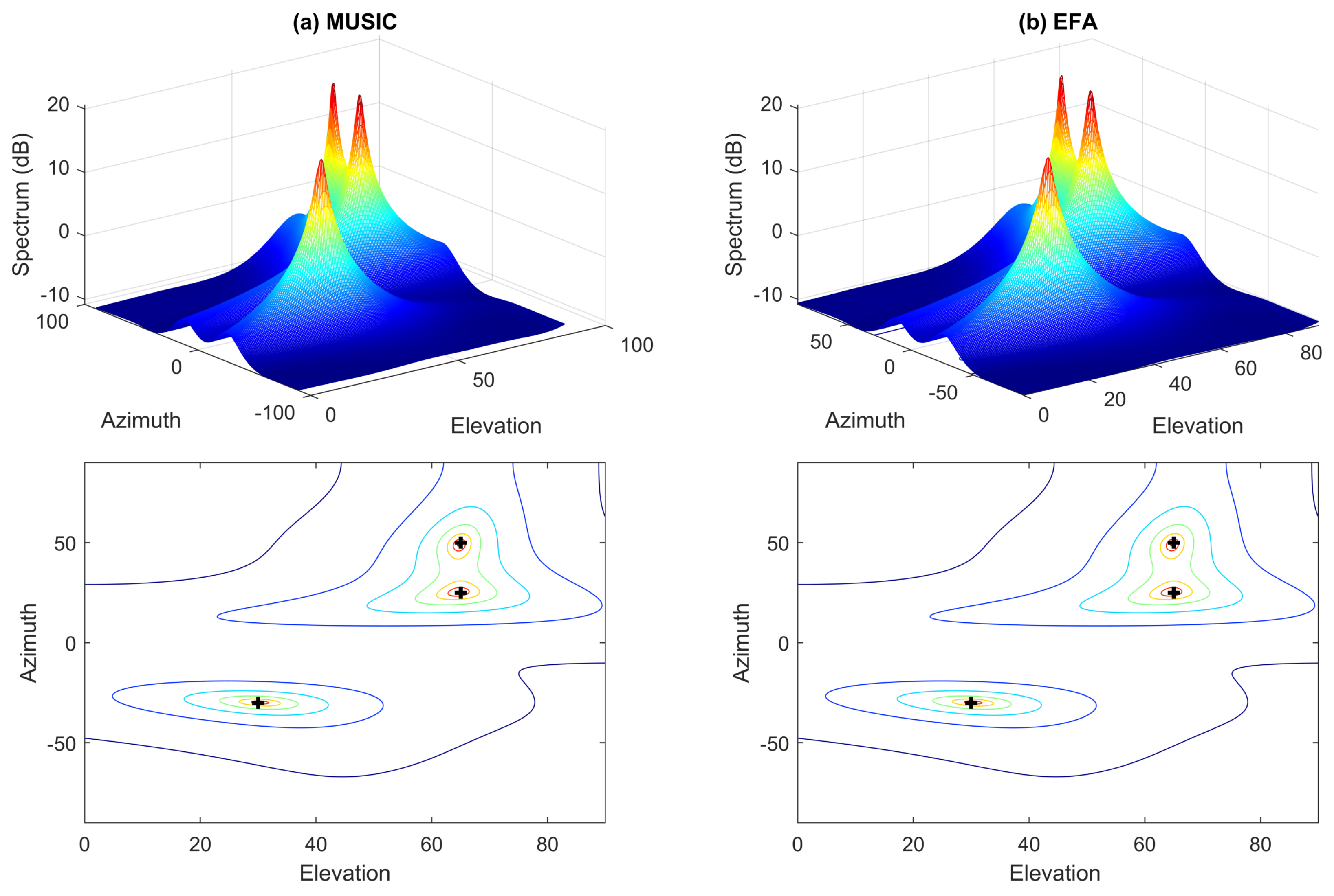
As a special case of nonuniform white noise, uniform white noise is considered in this example. Firstly, we assume that no outliers exist. The SNR is 10 dB. Figure 1 shows the resultant spectra and their contour plots of the MUSIC- and EFA-based approaches. It should be mentioned that in all simulations, the MUSIC algorithm is carried out by obtaining the subspace through the eigenvalue decomposition of the covariance matrix estimate, . From Figure 1, we notice that in such an ideal case, i.e., in uniform white noise and in the absence of data outliers, the two methods perform very well; the elevation as well as azimuth angles of the sources can be correctly estimated.
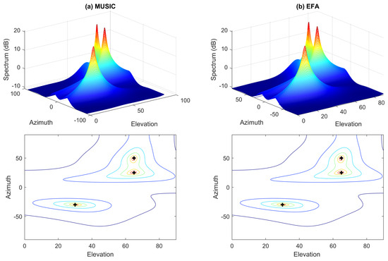
Figure 1.
Spectra and their contour plots of different methods in uniform white noise without outliers. Crosses denote the true DOAs. (a) left column: MUSIC; (b) right column: EFA.
5.2. Uniform White Noise with Outliers
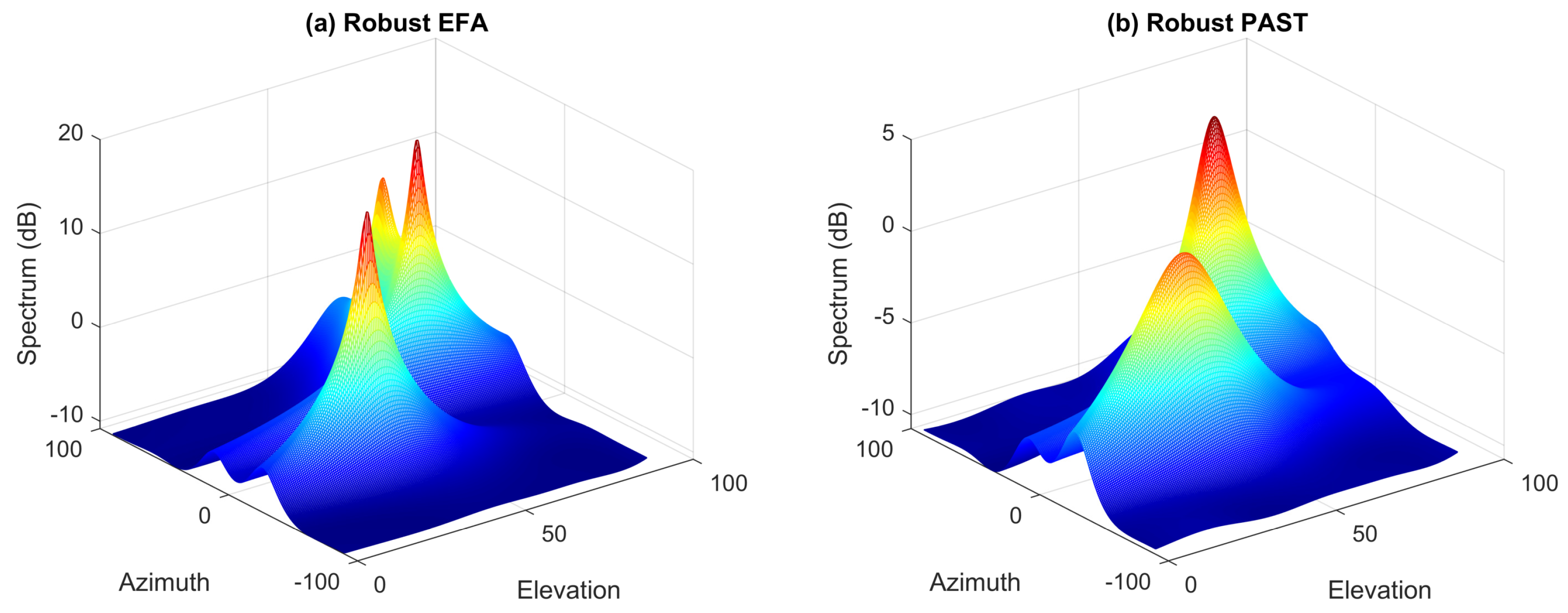
In this subsection, we assume that the data are corrupted by outliers. Figure 2a,b show the spectra and their contour plots of MUSIC and EFA in such a situation. It can be found that the data outliers can significantly deteriorate the performance of these nonrobust methods. Specifically, the spectra do not form proper peaks at the true DOAs. On the contrary, it can be seen from Figure 3a that the hostile effect of data outliers can be effectively suppressed by the proposed robust EFA method and hence, the DOAs can be still correctly estimated from the spectra. In the robust EFA method, the weight for the trimmed data point is set to . For comparison, the performance of the conventional robust PAST algorithm [18], where the forgetting factor is set to 0.95, is also tested and the corresponding result is shown in Figure 3b. We notice that the robust PAST algorithm also provide satisfactory performance in this case.
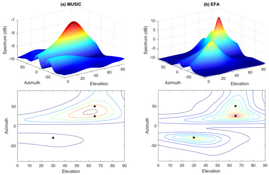
Figure 2.
Spectra and their contour plots of different methods in uniform white noise with outliers. Crosses denote the true DOAs. (a) left column: MUSIC; (b) right column: EFA.
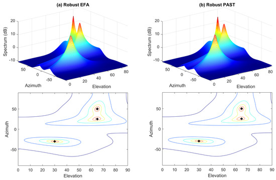
Figure 3.
Spectra and their contour plots of different methods in uniform white noise with outliers. Crosses denote the true DOAs. (a) left column: Robust EFA; (b) right column: Robust PAST.
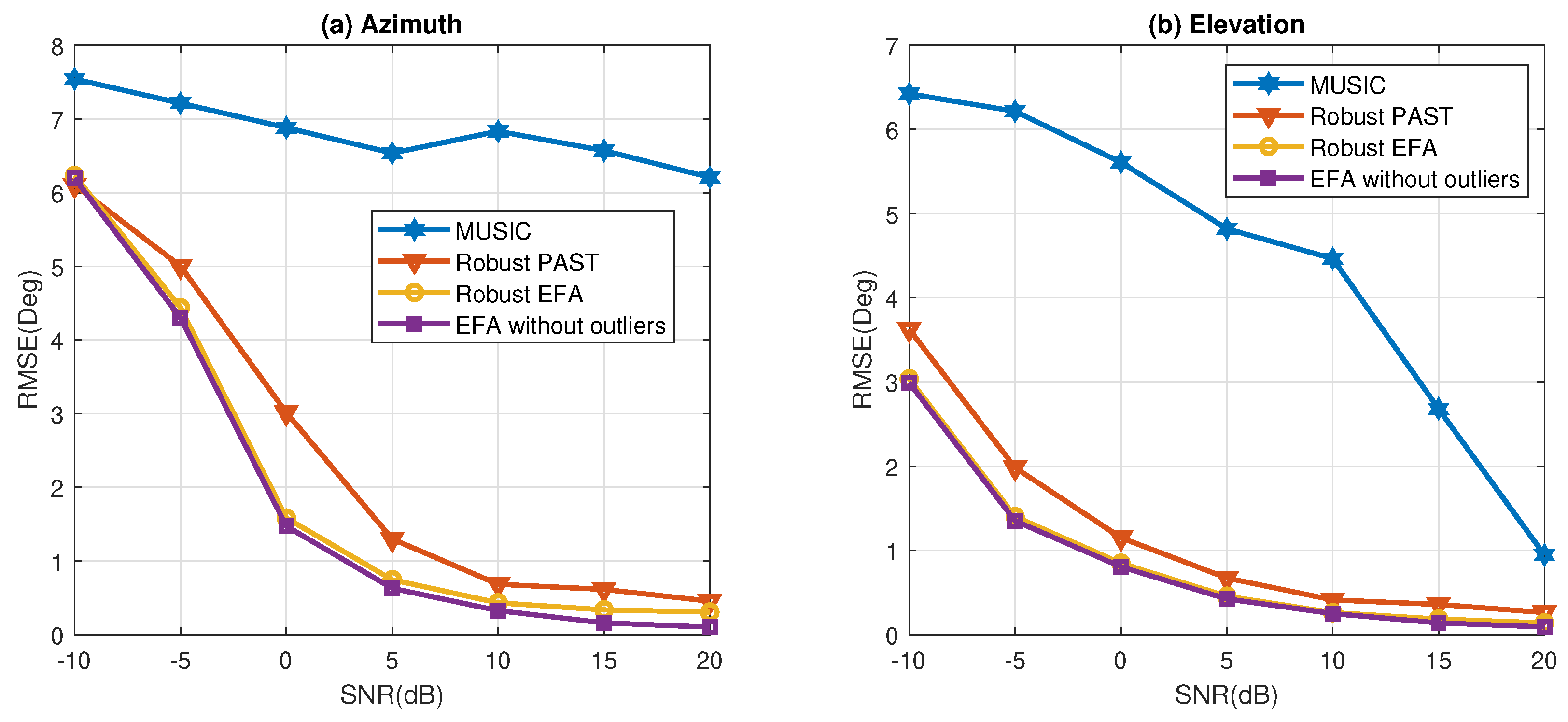
To further examine the performance of the robust EFA algorithm, the root-mean-square error (RMSE) of DOA estimation is compared with those of other methods (MUSIC and robust PAST) in Figure 4. The results are obtained from 100 independent runs. The performance of EFA without outliers is also shown as benchmark. It can be seen that the nonrobust MUSIC algorithm performs poorly in this scenario. Moreover, the proposed robust EFA algorithm generally outperforms the robust PAST algorithm. One reason is that the robust PAST algorithm does not update the subspace when the data are corrupted by outliers. In other words, the corrupted data are completely excluded for subspace estimation, and the number of effective snapshots in the robust PAST algorithm is less than that in the proposed method. In addition, it is found that the robust EFA algorithm is capable of achieving similar performance as the ideal case without outliers.
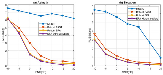
Figure 4.
RMSE of angle estimation in the uniform white noise with outliers (a) Azimuth angle; (b) Elevation angle.
It is also worth noting the robust PAST algorithm requires several snapshots to converge [18]. Hence, compared with the robust EFA algorithm, it may be further affected when the sample number is relatively small, or outliers exist in the first few snapshots. For illustration, we reduce the number of snapshots to 50, and the outliers occur at the th, th, th, and th entries of the data matrix. The resulting spectra of the robust PAST and robust EFA algorithms are shown in Figure 5. It is seen that the robust PAST algorithm does not perform well in this case, whereas the robust EFA algorithm still offer good performance.
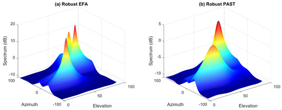
Figure 5.
Comparison of the spectra of robust EFA and robust PAST algorithms in the uniform white noise with outliers. The number of snapshots is 50.
5.3. Nonuniform White Noise without Outliers
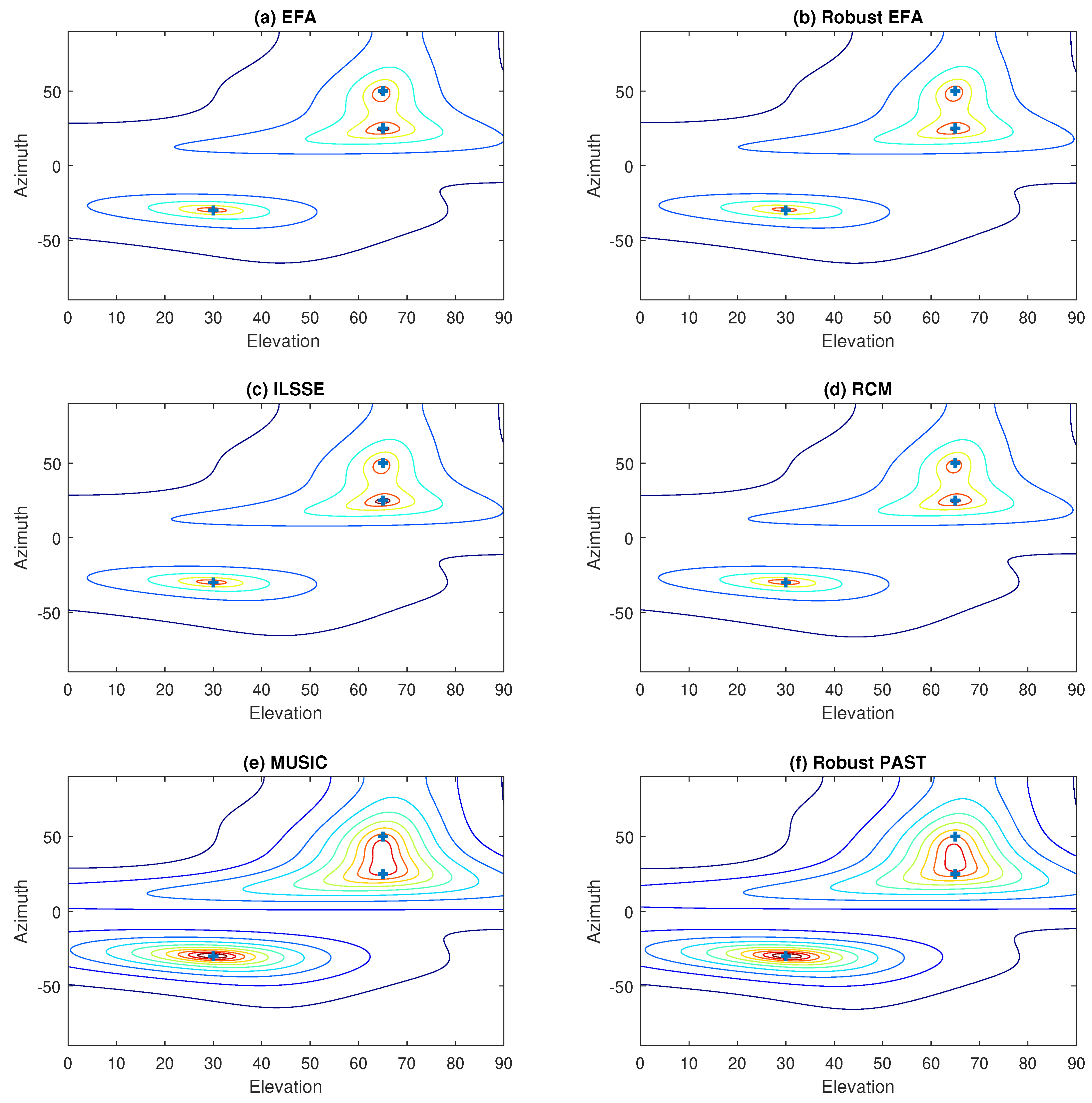
In this subsection, the noise is assumed to be nonuniform white. Firstly, we assume that there are no outliers in the data matrix . The SNR is 10 dB according to (46). Figure 6 shows the resultant contour plots of the spectra of various methods including EFA, robust EFA, ILSSE [9], reduced covariance matrix (RCM) [11], robust PAST [18], and MUSIC. Obviously, we can notice from Figure 6e,f that two peaks of the MUSIC spectrum and robust PAST spectrum are merged together. This is because in the nonuniform white noise environment, the subspace cannot be well estimated by these approaches. On the contrary, the EFA-based approaches (EFA and robust EFA), ILSSE, and RCM take the noise nonuniformity into account, so that the subspaces and DOAs can be properly determined.
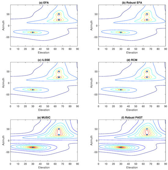
Figure 6.
Contour plots of the spectra of various methods in nonuniform white noise without outliers.
In Figure 7, the RMSEs of DOA estimation of different methods are compared. Since outliers are not considered in this example, the robust EFA and robust PAST are excluded, and we focus on comparing the performance of the proposed EFA-based method with the RCM and ILSSE algorithms. It is observed that when only nonuniform noise exists, the DOA estimation accuracy of these methods is similar, and the performance gap among these methods is small.
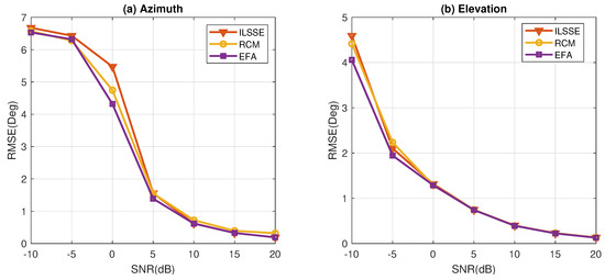
Figure 7.
Comparison of the RMSEs versus SNR in the nonuniform white noise without outliers.
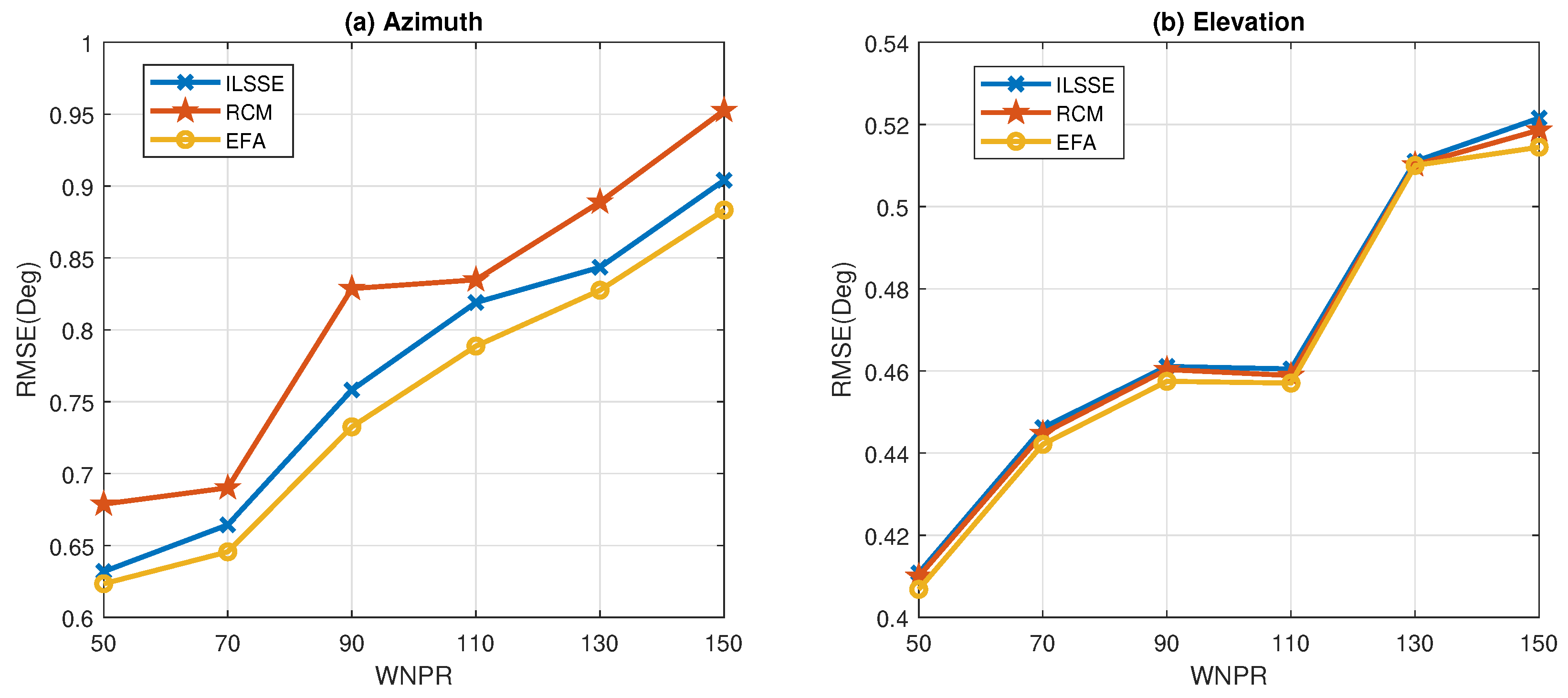
In order to examine the influence of the degree of the noise nonuniformity on DOA estimation, we change the maximum noise power, i.e., in (46), from 25 to 75, and keep . Therefore, the worst noise power ratio (WNPR), is varied from 50 to 150. For each WNPR, the SNR remains to be 10dB. It is seen from Figure 8 that the performance of all the tested methods degrades with the increase of WNPR. In general, the proposed EFA-based method achieves better performance than the other two methods.
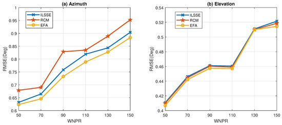
Figure 8.
Comparison of the RMSEs versus WNPR in the nonuniform white noise without outliers.
5.4. Nonuniform White Noise with Outliers
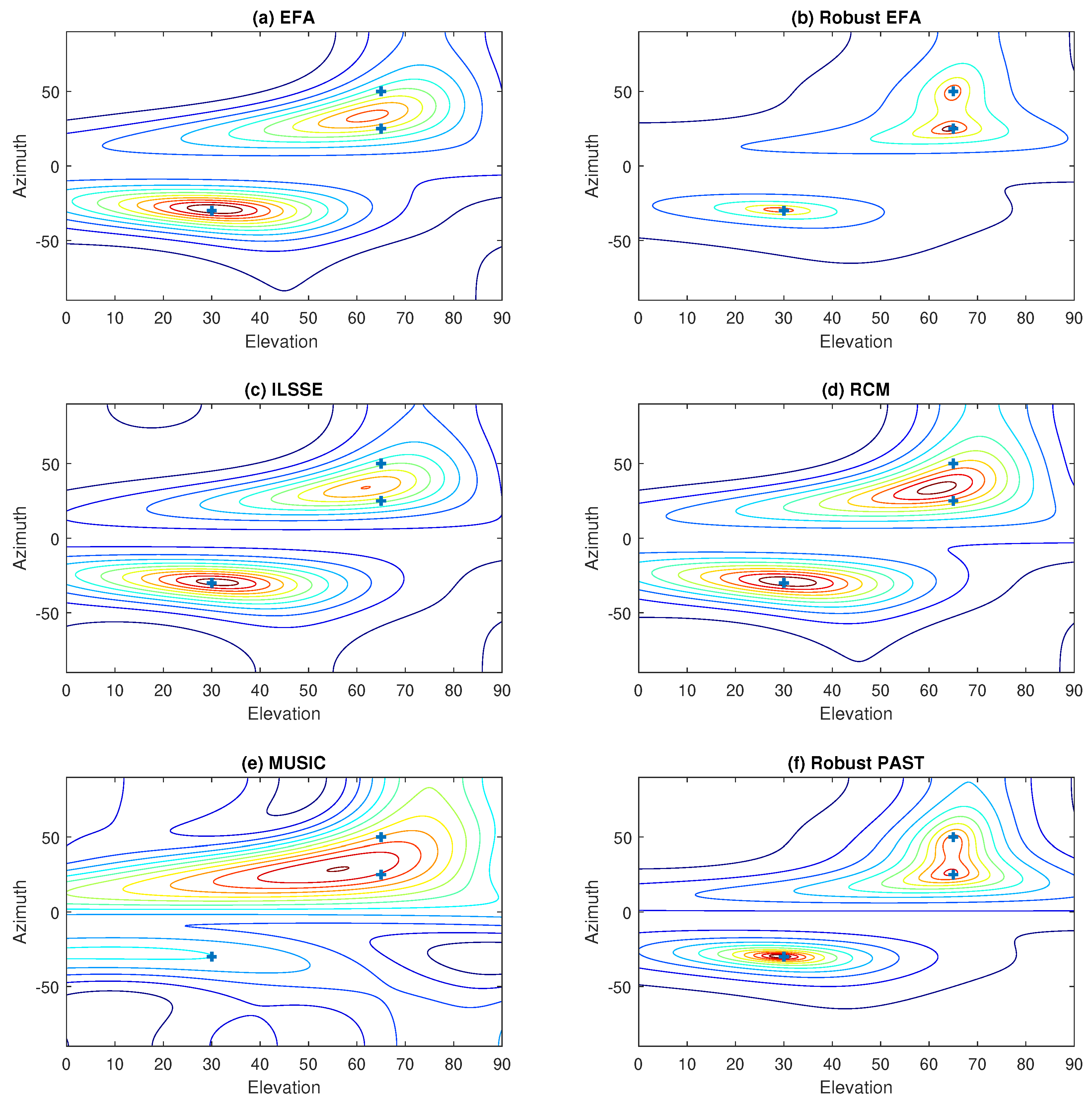
Following the previous setup, both noise nonuniformity and data outliers are considered. The resultant contour plots of the spectra of the proposed robust EFA algorithm and various conventional robust and nonrobust methods are shown in Figure 9. Obviously, it can be seen that the proposed robust EFA method can clearly identify the three source signals. As expected, the nonrobust methods, e.g., MUSIC, EFA, EFA, ILSSE, and RCM, are greatly affected by the outliers and they cannot provide satisfactory performance in this case. Furthermore, though the conventional robust PAST algorithm performs well in uniform noise with outliers, it does not offer satisfactory performance in nonuniform white noise. On the contrary, the issues of nonuniformity and data outliers can be simultaneously handled by the robust EFA method.
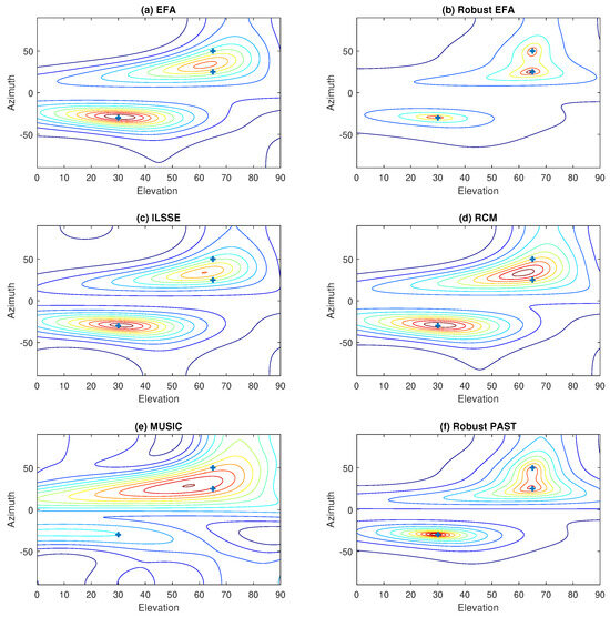
Figure 9.
Contour plots of the spectra of various methods in nonuniform white noise with outliers.
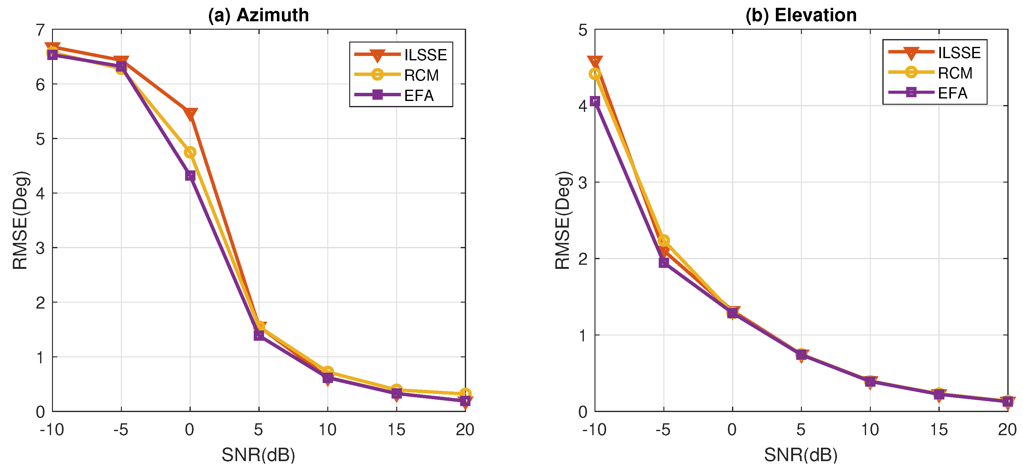
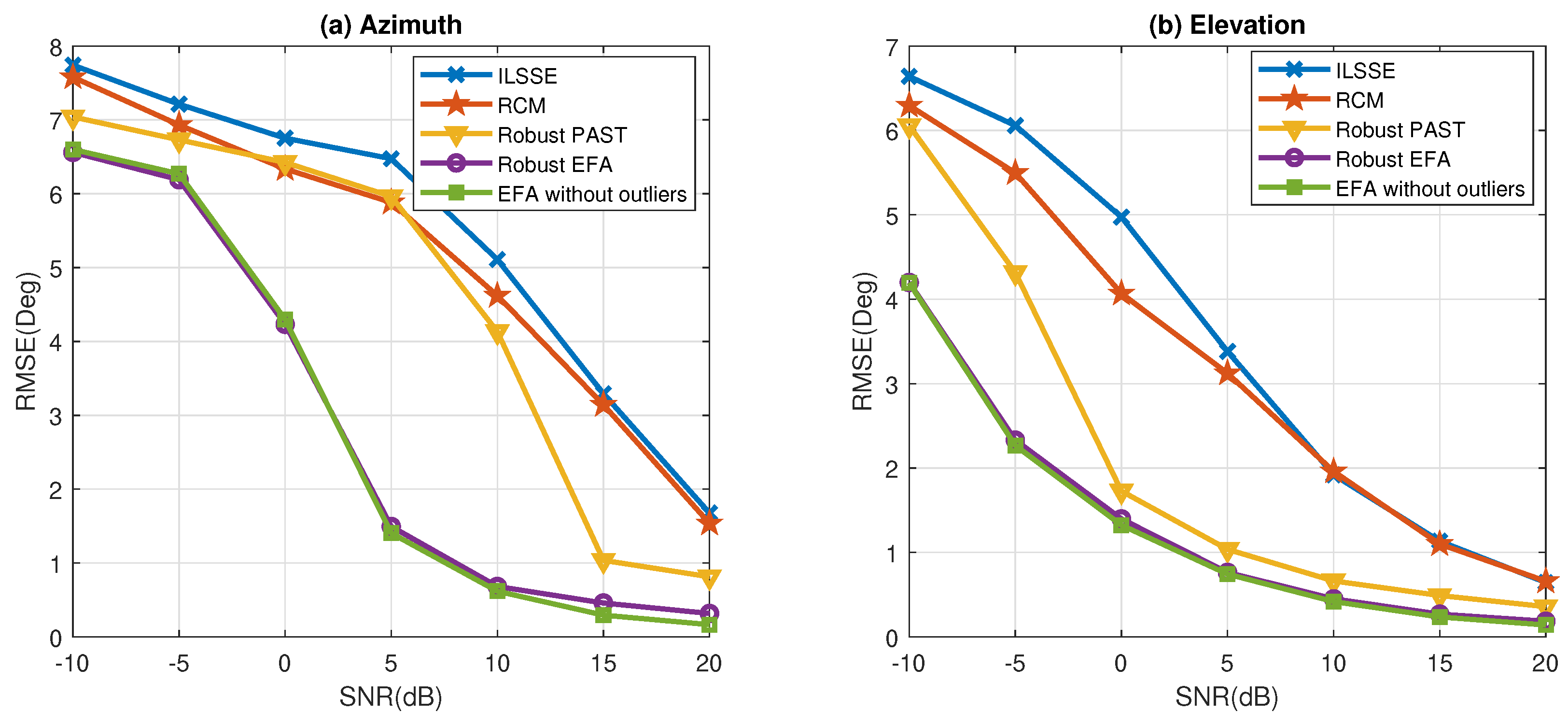
To further show the ability of the robust EFA against outliers, the RMSEs of azimuth and elevation estimation using this method are compared to various methods, including ILSSE, RCM, robust PAST, and the benchmark method (EFA without outliers) in Figure 10. We notice that the hostile effects of outliers can be successfully suppressed in all SNR levels tested, and the performance is quite closed to the case without outliers. Moreover, although the robust PAST algorithm is robust against outliers, it cannot suppress the nonuniform noise effectively, and hence, it is outperformed by the proposed method. For the ILSSE and RCM algorithms, although they can perform well in nonuniform noise, they cannot provide robustness against outliers and perform even worse than the robust PAST algorithm.

Figure 10.
Comparison of the RMSEs of angle estimation versus SNR in nonuniform white noise with outliers: (a) azimuth angle; (b) elevation angle.
6. Conclusions
In this paper, we investigate the problem of DOA estimation in the presence of nonuniform noise as well as data outliers. Differently to many traditional DOA estimation algorithms, which use a uniform white noise mode, it is assumed that the noise is nonuniform white noise, and the noise covariance matrix is diagonal but the diagonal elements are not identical. In order to estimate the subspace, and hence, DOAs, in this case, a new algorithm based on the EDA model is developed. Next, the data outliers are also considered. A simple method, i.e., the ESD test, is employed for outlier detection. Based on this detection, a trimmed data matrix can be obtained. According to the trimmed data matrix, a WLS problem is formulated to determine the subspace. Moreover, an iterative majorization approach, which is monotonic convergent, is introduced to solve the WLS problem. Simulation results show that the proposed robust DOA estimator outperforms traditional algorithms in the presence of nonuniform noise and outliers.
Author Contributions
Conceptualization, B.G. and B.L.; methodology, B.G. and B.L.; software, B.L. and X.S.; validation, B.G., X.S., Z.L. and B.L.; formal analysis, B.L., X.S. and B.L.; investigation, X.S., Z.L. and B.L.; resources, X.S. and Z.L.; writing—original draft preparation, B.G. and B.L.; writing—review and editing, B.G., X.S., Z.L. and B.L.;supervision, X.S. and Z.L.; project administration, X.S., Z.L. and B.L.; funding acquisition, X.S., Z.L. and B.L. All authors have read and agreed to the published version of the manuscript.
Funding
This work was funded in part by the National Natural Science Foundation of China under Grants 62171292 and 62101340, and in part by the Guangdong Basic and Applied Basic Research Foundation under Grant 2022A1515010188.
Data Availability Statement
The data presented in this study are available on request from the corresponding author.
Conflicts of Interest
Author Zhengqiang Li was employed by the company Shanghai Aircraft Design and Research Institute. The remaining authors declare that the research was conducted in the absence of any commercial or financial relationships that could be construed as a potential conflict of interest.
References
- Pesavento, M.; Gershman, A.B. Maximum-likelihood direction-of-arrival estimation in the presence of unknown nonuniform noise. IEEE Trans. Signal Process. 2001, 49, 1310–1324. [Google Scholar] [CrossRef]
- Böhme, J.F. Estimation of spectral parameters of correlated signals in wavefields. Signal Process. 1986, 11, 329–337. [Google Scholar] [CrossRef]
- Jaffer, A.G. Maximum likelihood direction finding of stochastic sources: A separable solution. In Proceedings of the ICASSP-88, International Conference on Acoustics, Speech, and Signal Processing, New York, NY, USA, 11–14 April 1988; pp. 2893–2894. [Google Scholar]
- Stoica, P.; Nehorai, A. On the concentrated stochastic likelihood function in array signal processing. Circuits Syst. Signal Process. 1995, 14, 669–674. [Google Scholar] [CrossRef]
- Stoica, P.; Viberg, M.; Wong, K.M.; Wu, Q. Maximum-likelihood bearing estimation with partly calibrated arrays in spatially correlated noise fields. IEEE Trans. Signal Process. 1996, 44, 888–899. [Google Scholar] [CrossRef]
- Chen, C.E.; Lorenzelli, F.; Hudson, R.E.; Yao, K. Stochastic maximum-likelihood DOA estimation in the presence of unknown nonuniform noise. IEEE Trans. Signal Process. 2008, 56, 3038–3044. [Google Scholar] [CrossRef]
- Wu, Y.; Hou, C.; Liao, G.; Guo, Q. Direction-of-arrival estimation in the presence of unknown nonuniform noise fields. IEEE J. Ocean. Eng. 2006, 31, 504–510. [Google Scholar] [CrossRef]
- Liao, B.; Liao, G.; Wen, J. A method for DOA estimation in the presence of unknown nonuniform noise. J. Electromagn. Waves Appl. 2008, 22, 2113–2123. [Google Scholar] [CrossRef]
- Liao, B.; Chan, S.C.; Huang, L.; Guo, C. Iterative methods for subspace and DOA estimation in nonuniform noise. IEEE Trans. Signal Process. 2016, 64, 3008–3020. [Google Scholar] [CrossRef]
- Liao, B.; Wen, J.; Huang, L.; Guo, C.; Chan, S.C. Direction finding with partly calibrated uniform linear arrays in nonuniform noise. IEEE Sens. J. 2016, 16, 4882–4890. [Google Scholar] [CrossRef]
- Liao, B.; Huang, L.; Guo, C.; So, H.C. New approaches to direction-of-arrival estimation with sensor arrays in unknown nonuniform noise. IEEE Sens. J. 2016, 16, 8982–8989. [Google Scholar] [CrossRef]
- Wen, J.; Liao, B.; Guo, C. Spatial smoothing based methods for direction-of-arrival estimation of coherent signals in nonuniform noise. Digit. Signal Process. 2017, 67, 116–122. [Google Scholar] [CrossRef]
- Liao, B.; Guo, C.; Huang, L.; Wen, J. Matrix completion based direction-of-arrival estimation in nonuniform noise. In Proceedings of the 2016 IEEE International Conference on Digital Signal Processing (DSP), Beijing, China, 16–18 October 2016; pp. 66–69. [Google Scholar]
- Fang, Y.; Zhu, S.; Zeng, C.; Gao, Y.; Li, S. DOA Estimations with Limited Snapshots Based on Improved Rank-One Correlation Model in Unknown Nonuniform Noise. IEEE Trans. Veh. Technol. 2021, 70, 10308–10319. [Google Scholar] [CrossRef]
- Xu, H.; Jin, M.; Guo, Q.; Jiang, T.; Tian, Y. Direction of Arrival Estimation with Gain-Phase Uncertainties in Unknown Nonuniform Noise. IEEE Trans. Aerosp. Electron. Syst. 2023, 59, 9686–9696. [Google Scholar] [CrossRef]
- Kozick, R.J.; Sadler, B.M. Maximum-likelihood array processing in non-Gaussian noise with Gaussian mixtures. IEEE Trans. Signal Process. 2000, 48, 3520–3535. [Google Scholar]
- Lim, C.H.; See, S.C.M.; Zoubir, A.M.; Ng, B.P. Robust adaptive trimming for high-resolution direction finding. IEEE Signal Process. Lett. 2009, 16, 580–583. [Google Scholar]
- Chan, S.C.; Wen, Y.; Ho, K.L. A robust past algorithm for subspace tracking in impulsive noise. IEEE Trans. Signal Process. 2005, 54, 105–116. [Google Scholar] [CrossRef]
- Huber, P.J. Robust Statistics; John Wiley & Sons: Hoboken, NJ, USA, 2004; Volume 523. [Google Scholar]
- Zou, Y.; Chan, S.; Ng, T. A recursive least M-estimate (RLM) adaptive filter for robust filtering in impulse noise. IEEE Signal Process. Lett. 2000, 7, 324–326. [Google Scholar] [CrossRef]
- Zou, Y.; Chan, S.C.; Ng, T.S. Fast least mean M-estimate algorithms for robust adaptive filtering in impulse noise. In Proceedings of the 2000 10th European Signal Processing Conference, Tampere, Finland, 4–8 September 2000; pp. 1–4. [Google Scholar]
- Yang, B. Projection approximation subspace tracking. IEEE Trans. Signal Process. 1995, 43, 95–107. [Google Scholar] [CrossRef]
- Mardia, K.; Kent, J.; Bibby, J. Multivariate Analysis (Probability and Mathematical Statistics); Academic Press: Cambridge, MA, USA, 1980. [Google Scholar]
- McDonald, R.P. The simultaneous estimation of factor loadings and scores. Br. J. Math. Stat. Psychol. 1979, 32, 212–228. [Google Scholar] [CrossRef]
- Knott, M.; Bartholomew, D.J. Latent Variable Models and Factor Analysis; Edward Arnold: New York, NY, USA, 1999. [Google Scholar]
- Trendafilov, N.T.; Unkel, S. Exploratory factor analysis of data matrices with more variables than observations. J. Comput. Graph. Stat. 2011, 20, 874–891. [Google Scholar] [CrossRef]
- Unkel, S.; Trendafilov, N.T. Simultaneous parameter estimation in exploratory factor analysis: An expository review. Int. Stat. Rev. 2010, 78, 363–382. [Google Scholar] [CrossRef]
- Rosner, B. Percentage points for a generalized ESD many-outlier procedure. Technometrics 1983, 25, 165–172. [Google Scholar] [CrossRef]
- Kiers, H.A. Weighted least squares fitting using ordinary least squares algorithms. Psychometrika 1997, 62, 251–266. [Google Scholar] [CrossRef]
- Gower, J.C.; Dijksterhuis, G.B. Procrustes Problems; Oxford University Press: Oxford, UK, 2004. [Google Scholar]
- Osborne, J.W.; Overbay, A. The power of outliers (and why researchers should always check for them). Pract. Assess. Res. Eval. 2019, 9, 6. [Google Scholar]
- Barnett, V.; Lewis, T. Outliers in Statistical Data; Wiley: New York, NY, USA, 1994. [Google Scholar]
- Hawkins, D.M. Identification of Outliers; Springer: Berlin/Heidelberg, Germany, 1980; Volume 11. [Google Scholar]
- Hodge, V.; Austin, J. A survey of outlier detection methodologies. Artif. Intell. Rev. 2004, 22, 85–126. [Google Scholar] [CrossRef]


Disclaimer/Publisher’s Note: The statements, opinions and data contained in all publications are solely those of the individual author(s) and contributor(s) and not of MDPI and/or the editor(s). MDPI and/or the editor(s) disclaim responsibility for any injury to people or property resulting from any ideas, methods, instructions or products referred to in the content. |
© 2024 by the authors. Licensee MDPI, Basel, Switzerland. This article is an open access article distributed under the terms and conditions of the Creative Commons Attribution (CC BY) license (https://creativecommons.org/licenses/by/4.0/).