A Novel Mamba Architecture with a Semantic Transformer for Efficient Real-Time Remote Sensing Semantic Segmentation

Abstract

Real-time remote sensing segmentation technology is crucial for unmanned aerial vehicles (UAVs) in battlefield surveillance, land characterization observation, earthquake disaster assessment, etc., and can significantly enhance the application value of UAVs in military and civilian fields. To realize this potential, it is essential to develop real-time semantic segmentation methods that can be applied to resource-limited platforms, such as edge devices. The majority of mainstream real-time semantic segmentation methods rely on convolutional neural networks (CNNs) and transformers. However, CNNs cannot effectively capture long-range dependencies, while transformers have high computational complexity. This paper proposes a novel remote sensing Mamba architecture for real-time segmentation tasks in remote sensing, named RTMamba. Specifically, the backbone utilizes a Visual State-Space (VSS) block to extract deep features and maintains linear computational complexity, thereby capturing long-range contextual information. Additionally, a novel Inverted Triangle Pyramid Pooling (ITP) module is incorporated into the decoder. The ITP module can effectively filter redundant feature information and enhance the perception of objects and their boundaries in remote sensing images. Extensive experiments were conducted on three challenging aerial remote sensing segmentation benchmarks, including Vaihingen, Potsdam, and LoveDA. The results show that RTMamba achieves competitive performance advantages in terms of segmentation accuracy and inference speed compared to state-of-the-art CNN and transformer methods. To further validate the deployment potential of the model on embedded devices with limited resources, such as UAVs, we conducted tests on the Jetson AGX Orin edge device. The experimental results demonstrate that RTMamba achieves impressive real-time segmentation performance.

1. Introduction

Real-time remote sensing semantic segmentation is a critical task for unmanned aerial vehicle (UAV) applications, aiming to classify each pixel in images into categories like buildings, roads, vegetation, etc. [1,2]. This enables UAVs to perform real-time segmentation without offline processing, which is crucial for emergency scenarios such as disaster response and military operations. The task must be executed on edge computing devices like embedded GPUs in UAVs, necessitating segmentation models with low parameter counts, minimal power consumption, and high computational efficiency.

Deep learning [3] has revolutionized remote sensing semantic segmentation [4]. Fully convolutional networks (FCNs) [5] excel in hierarchical feature learning. Encoder–decoder architectures like U-Net [6] introduce refined upsampling and skip connections. DeeplabV3+ [7] and PSPNet [8] improve multiscale feature capture. Recent methods like BiseNet [9] and BiseNetv2 [10] optimize latency, feature extraction, and efficiency, emphasizing real-time performance. The high computational costs of complex networks have shifted the focus to lightweight networks. GAGNet [11] utilizes a novel lightweight student network framework for remote sensing segmentation tasks. DDRNet [12] balances speed and precision with multi-stage fusion. DSANet [13] uses lightweight attention for faster processing. TransUNet [14] and UNetFormer [15] integrate the transformer architecture with a UNet framework. PIDNet [16] and SCTNet [17] offer new solutions for real-time segmentation tasks. Hybrid CNN and transformer architectures face limitations: CNNs have a limited receptive field, while transformers’ self-attention is computationally expensive. State-space models (SSMs), such as Mamba [18], are promising for sequence modeling and excel in language and visual tasks. Mamba’s success has extended to remote sensing. RSMamba [19] is an efficient model for remote sensing image classification, while Remote Sensing Mamba (RSM) [20] handles dense prediction tasks. In particular, RS3Mamba [21] was the first to introduce the visual state-space model into remote sensing semantic segmentation, although it did not emphasize real-time performance. Although the above methods have achieved significant success in the field of remote sensing image segmentation, complex scene content in remote sensing images often contains a considerable amount of noise and redundant feature information. Thus, achieving effective filtering of this information to strike a balance between speed and accuracy is a process that requires further exploration. Therefore, to address the aforementioned issues, this paper explores the potential of state-space models (SSMs) in real-time remote sensing segmentation for UAVs.

To address these challenges and leverage the strengths of SSMs, this paper proposes RTMamba, a novel architecture for real-time semantic segmentation in remote sensing. RTMamba comprises three main components: the backbone, the decoder, and a semantic transformer. The backbone uses CNNs for shallow feature capture and VSS blocks for deep features and long-range dependencies, reducing computational complexity. The decoder predicts feature masks and includes an Inverted Triangle Pyramid Pooling (ITP) module to filter redundant information and enhance multiscale object perception. The semantic transformer used only during training provides semantic and spatial details to the backbone and decoder. During inference, RTMamba retains only the backbone and decoder, ensuring a lightweight architecture. Experiments on three aerial remote sensing datasets show that RTMamba balances accuracy and speed better than previous models. Speed tests on the Jetson AGX Orin [22] edge device confirm RTMamba’s robust real-time performance.

The main contributions of the proposed RTMamba can be summarized as follows:

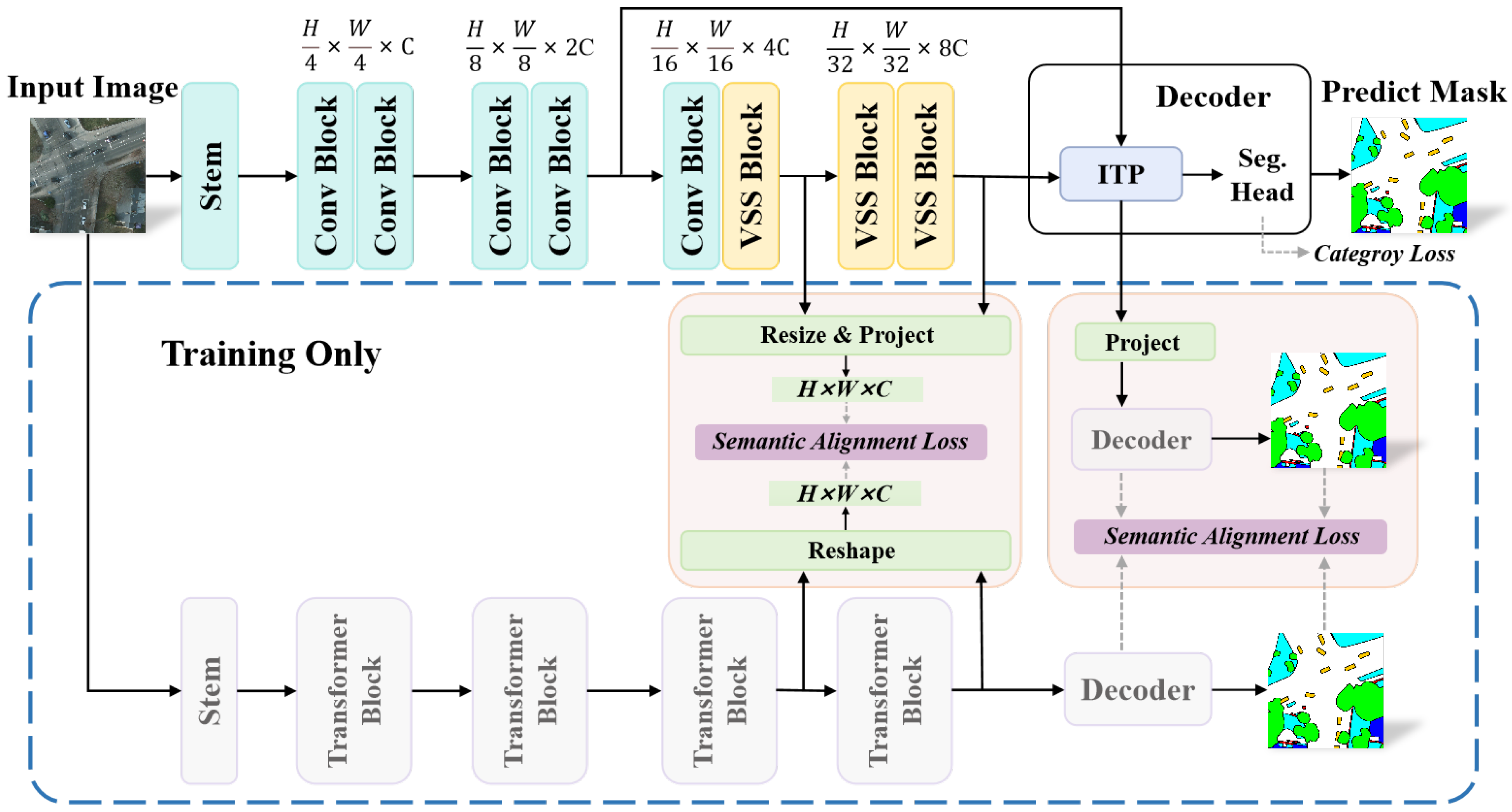
• In this paper, we propose a novel remote sensing Mamba architecture for real-time semantic segmentation tasks, named RTMamba. The backbone section leverages VSS blocks to exploit their potential in remote sensing semantic segmentation. During inference, only the backbone and decoder are retained, ensuring a lightweight design.
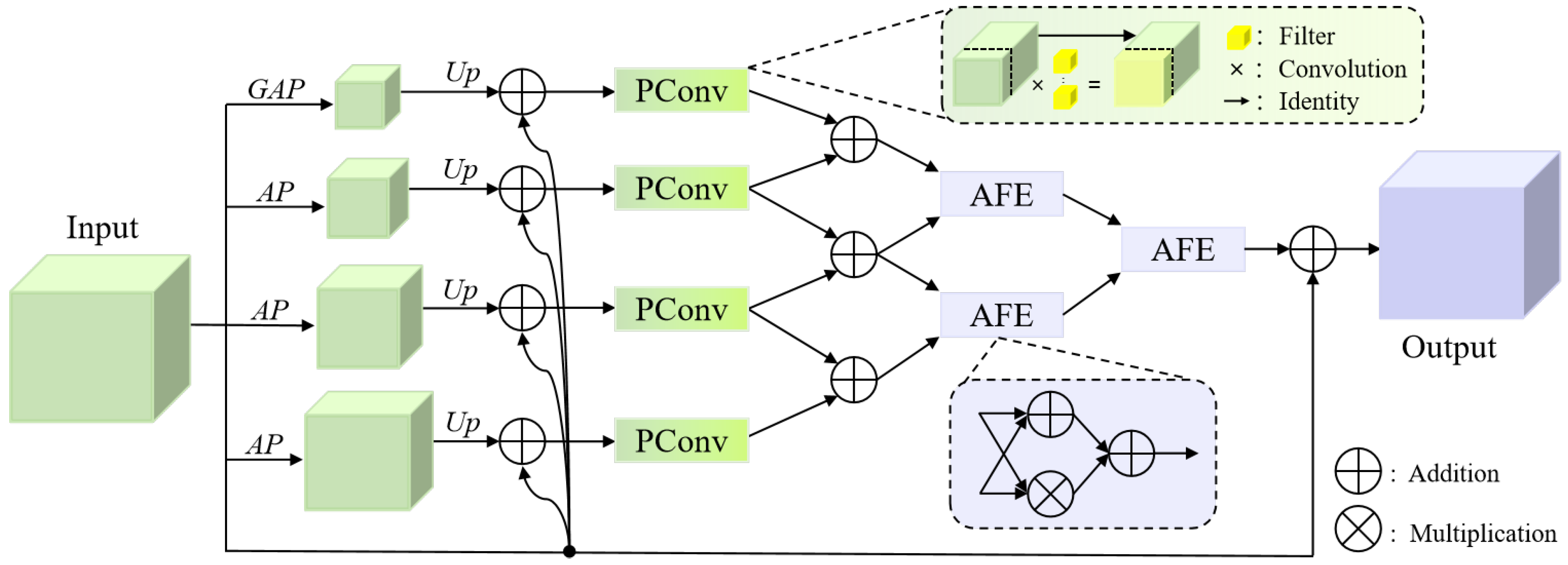
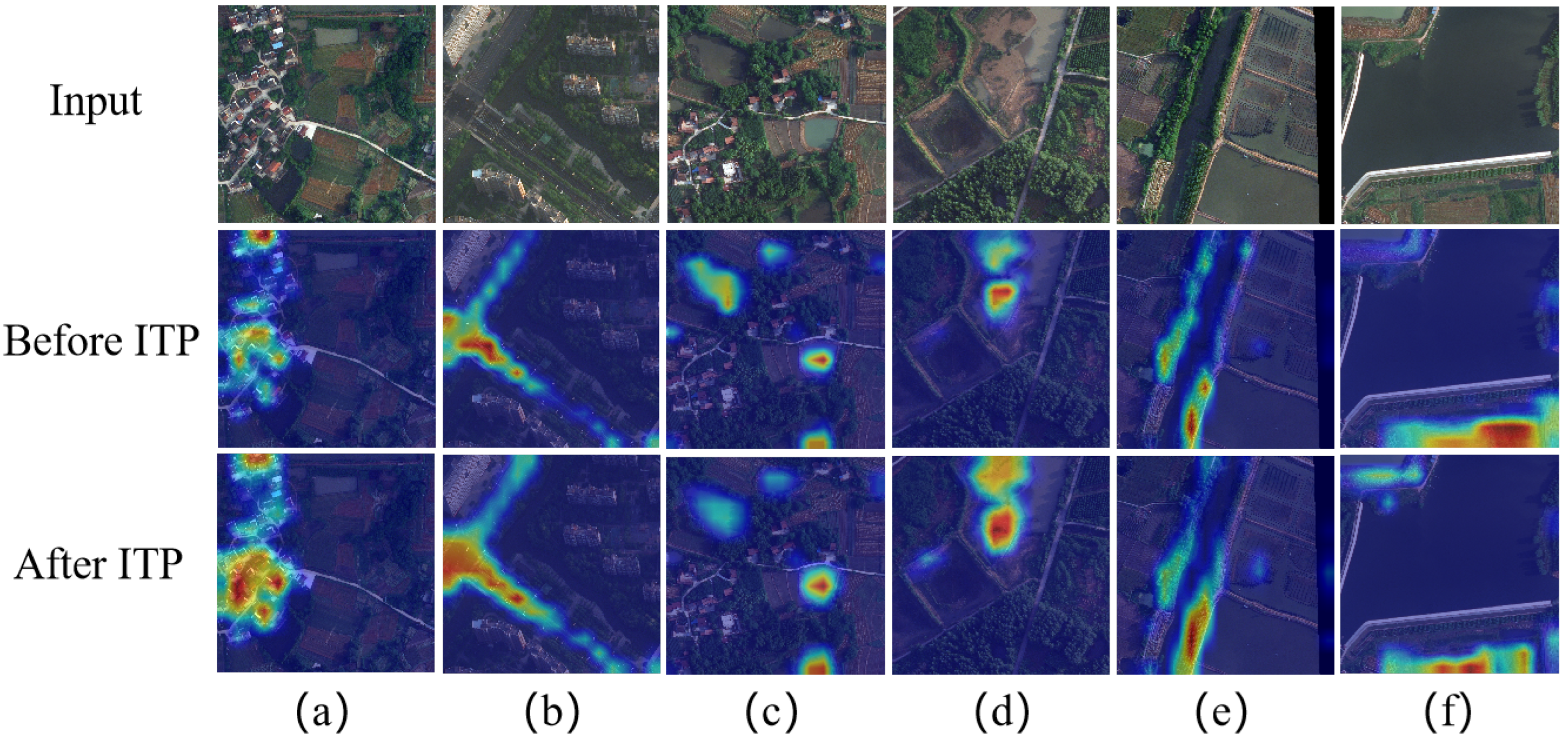
• To address the issue of redundant features from the backbone input to the decoder, we design a novel Inverted Triangle Pyramid Pooling (ITP) module. The ITP module effectively utilizes multiscale features, filtering redundant information and enhancing the perception capability of objects and their boundaries in remote sensing images.
• Extensive experiments are conducted on three well-known remote sensing datasets: Vaihingen, Potsdam, and LoveDA. The results illustrate that RTMamba exhibits competitive performance advantages compared to existing state-of-the-art CNN and transformer methods. Additionally, testing on the Jetson AGX Orin edge device further underscores the potential application prospects of RTMamba in real-time remote sensing segmentation tasks for UAVs.

2. Related Works

2.1. Semantic Segmentation

Semantic segmentation, as a fundamental task of environmental perception, has attracted significant attention from researchers in the field [1]. Ref. [4] proposed a new segmentation algorithm based on the Markov random-field model. Fully convolutional networks (FCNs) [5], which are derived from convolutional neural networks (CNNs), excel in hierarchical feature learning and have pioneered the field. However, alternative approaches have emerged, such as encoder–decoder architectures. For example, SegNet [23] uses max-pooling indices for refined upsampling during decoding, while U-Net [6] integrates skip connections for effective layer linkage. To effectively capture multiscale object features, DeepLab [7] utilizes the atrous spatial pyramid pooling (ASPP) module. On the other hand, PSPNet [8] incorporates a pyramid pooling module to achieve context integration. Recent advancements, such as BiseNet [9], optimize low latency and spatial-contextual feature extraction. BiseNetV2 [10] improves information flow through bidirectional aggregation. These methods have significantly advanced the field of semantic segmentation, particularly in the domain of remote sensing image segmentation [2]. Currently, the remote sensing semantic segmentation task is increasingly focused on real-time performance, and an increasing number of researchers are investigating real-time semantic segmentation tasks for remote sensing images.

2.2. Real-Time Semantic Segmentation of Remote Sensing Images

Real-time semantic segmentation in remote sensing faces a trade-off between speed and precision. Existing methods address this challenge using various approaches. GAGNet [11] utilizes a novel lightweight student network framework for remote sensing segmentation tasks. This framework is guided by a graph attention mechanism with knowledge extraction capabilities. DDRNet [12] addresses this challenge with a novel context extractor employing multi-stage fusion, effectively balancing speed and precision. MANet [24] utilizes a multi-aggregation network for remote sensing image segmentation. Additionally, DSANet [13] integrates a lightweight attention mechanism for faster processing of large remote sensing images. PIDNet [16] and SCTNet [17] offer new solutions for real-time segmentation tasks. Moreover, UNetFormer [15] integrates the transformer architecture into a UNet-inspired framework, demonstrating its effectiveness in remote sensing image segmentation. These advances pave the way for the broader application of real-time semantic segmentation in remote sensing tasks, thereby enabling more efficient and accurate monitoring and analysis of the Earth’s surface.

2.3. State-Space Models and Applications

State-space models (SSMs), particularly exemplified by Mamba [18], have emerged as promising architectures for sequence modeling. They can efficiently handle long-range dependencies and offer solutions to challenges in various domains. Mamba has not only achieved success in language modeling but also in visual tasks. DenseMamba [25] preserves fine-grained information, essential for output quality. Vim [26] and VMamba [27] introduce bidirectional SSM blocks and the Cross-Scan Module (CSM) for efficient visual representation learning. MotionMamba [28] introduces innovative motion generation techniques using hierarchical temporal and bidirectional spatial Mamba blocks. Moreover, Mamba has attracted the attention of researchers in the field of remote sensing. RSMamba [19] is an efficient state-space model for remote sensing image classification. Ref. [20] proposed a method called Remote Sensing Mamba (RSM) based on the state-space model, which effectively accomplishes dense prediction tasks. RS3Mamba [21] incorporates the visual state-space model into remote sensing semantic segmentation and features a dual-branch network. In conclusion, the integration of SSMs (especially Mamba) represents a significant advancement in sequence modeling, providing effective solutions for handling long-term dependencies in various applications. This paper continues the examination of potential applications of SSMs in real-time segmentation in remote sensing.

3. Methods

3.1. Preliminary: State-Space Model

State-space models represent dynamic systems using first-order differential or difference equations to describe the internal state evolution and their relationship to outputs. This matrix-vector approach, expressed through equations, facilitates the analysis of multivariable systems. In particular, a sequence $x(t)\in {\mathbb{R}}^L$ is mapped to $y(t)\in {\mathbb{R}}^L$ through the hidden state $h(t)\in {\mathbb{R}}^N$. The formula is as follows:

$$h^{\prime }(t)=Ah(t)+Bx(t)$$

(1)

$$y(t)=Ch(t)+Dx(t)$$

(2)

where $A\in {\mathbb{R}}^{N\times N}$ represents the evolution parameters. $B\in {\mathbb{R}}^N$ and $C\in {\mathbb{R}}^N$ are the projection parameters. $D\in {\mathbb{R}}^1$ represents the skip connection.

3.2. RTMamba Architecture

The proposed RTMamba follows a similar architecture to SCTNet [17], as shown in Figure 1. RTMamba follows a single-branch structure during inference. During training, a semantic transformer is introduced to provide rich semantic information and spatial detail information. Specifically, RTMamba consists of a backbone, a decoder, and a semantic transformer.

The components of the RTMamba architecture are as follows:

(1) Backbone: In our architecture, we employ a CNN for initial feature extraction in the shallow layers of the backbone. For deeper feature coding, we utilize a VSS block, maintaining linear complexity while capturing long-range contextual information. This enhances feature representation, which is especially beneficial for high-resolution images in remote sensing tasks. The input features $X\in {\mathbb{R}}^{H\times W\times 3}$ are processed initially via a stem block with consecutive $3\times 3$ convolutional layers, followed by stacked residual blocks for shallow feature extraction, producing features of size ${\displaystyle \frac{H}{4}}\times {\displaystyle \frac{W}{4}}\times C,{\displaystyle \frac{H}{8}}\times {\displaystyle \frac{W}{8}}\times 2C$. In the last two stages, deep feature correlation extraction is conducted using two VSS blocks, yielding features of size ${\displaystyle \frac{H}{16}}\times {\displaystyle \frac{W}{16}}\times 4C,{\displaystyle \frac{H}{32}}\times {\displaystyle \frac{W}{32}}\times 8C$. During training, features from these stages are jointly learned with those from the semantic transformer, enabling the backbone to enhance semantic and spatial detail information.

(2) Decoder: The decoder incorporates the ITP module and segmentation heads. Our novel ITP module serves as the feature interaction module, effectively filtering redundant features and enhancing object perception in remote sensing images. It accepts feature maps from the backbone’s second stage. The segmentation head is straightforward, comprising a $3\times 3$ convolutional layer, BN, ReLU activation, and a $1\times 1$ convolutional classifier. During training, the decoder aligns features with the semantic transformer for loss computation.

(3) Semantic Transformer: The semantic transformer part follows the design of SCTNet [17]. During training only, the features obtained in the third and fourth stages are aligned and interactively learned with the corresponding features of the backbone in the corresponding stages. In addition, in the decoder part of the semantic transformer, the predicted results also participate in the alignment with the decoder for joint learning. In this context, we employ the CWD loss [29] as our semantic alignment loss function.

3.3. VSS Block

The recent emergence of SSMs has attracted widespread attention among researchers. In VMamba [27], the state-space model is extended to the visual domain. Inspired by VMamba, we introduce a VSS block into the backbone of RTMamba as a module for deep feature processing. It is capable of capturing long-range contextual information while maintaining linear complexity. Furthermore, the VSS block enhances the acquisition of refined semantic information. During the training phase, the VSS block undergoes feature interaction training with the semantic transformer. The semantic alignment loss guides the VSS block to focus on capturing more semantically meaningful features that align well with the semantic transformer’s understanding. Specifically, as illustrated in Figure 2, the input features are split into two paths after layer normalization.

One path sequentially traverses through a linear layer, depth-wise convolution, 2D selective scanning (SS2D) operation, and layer normalization to obtain the features. Another path simply passes through a linear layer, and then the results of the two paths are fused by element-wise multiplication. Finally, the output of the VSS block is obtained by connecting the result to the original features through a linear layer using a residual connection. The formula is as follows:

$$Q_x=f^{LN}(x)$$

(3)

$$S_x=f^{LN}(f^{SS2D}(D^{conv}(f^{Linear}(Q_x))))\odot Q_x$$

(4)

$$F_x^{VSS}=f^{Linear}(S_x)+x$$

(5)

where x represents the input features. $f^{LN}(·)$ is the layer normalization operation. $f^{Linear}(·)$ is the linear transform operation. $D^{conv}(·)$ is the depth-wise convolution operation. ⊙ is the element-wise multiplication operation. $f^{SS2D}(·)$ is the 2D selective scanning operation. $F_x^{VSS}$ represents the result obtained by processing the input feature x through the VSS block. During the training phase, the result obtained after processing through the VSS block is projected with the corresponding stage of the semantic transformer. Semantic alignment loss is later applied during the training phase to help the backbone effectively learn both semantic and spatial detail information.

The core of the VSS block is the 2D selective scanning (SS2D) structure, as shown in Figure 3.

To enlarge the receptive field without increasing computational complexity, forward or backward scanning of the image is implemented. This involves expanding the image along four directions to obtain four different sequences, which are then processed by S6 [27]. The S6 operation allows each element in the one-dimensional array to interact with all previously scanned samples through compressed hidden states, capturing different features. The pseudo-code for the S6 operation is presented in Algorithm 1.

Algorithm 1: S6 operation in SS2D: Pseudo-code

Input: x, a feature tensor of shape [B, L, D]   (batch size, sequence length, dimension)   Parameters:A, D, nn.Parameters   Operator: Linear(.), a linear projection layer Output: y, the feature tensor of shape [B, L, D]   1: $\mathrm{\Delta },B,C=\mathrm{Linear}(x),\mathrm{Linear}(x),\mathrm{Linear}(x)$   2: $\overline{A}=exp(\mathrm{\Delta }A)$   3: $\overline{B}={(\mathrm{\Delta }A)}^{-1}(exp(\mathrm{\Delta }A)-I)·\mathrm{\Delta }B$   4: $h_t=\overline{A}{h}_{t-1}+\overline{B}{x}_t$   5: $y_t=C{h}_t+D{x}_t$   6: $y=[y_1,y_2,\dots ,y_t,\dots ,y_L]$   7: return y

Finally, the output image is restored to its original size through scan merging. The formula is as follows:

$$X_O=S^{se}(x,O)$$

(6)

$$\widehat{X_O}=S6(X_O)$$

(7)

$$X_{ss2d}=S^{sm}(\widehat{X_{(1)}},\widehat{X_{(2)}},\widehat{X_{(3)}},\widehat{X_{(4)}})$$

(8)

where O stands for the different directions, $O\in [1,2,3,4]$. x denotes the input features. $S^{se}(·)$ and $S^{sm}(·)$ represent the scan expanding and scan merging operations, respectively. $S6(·)$ represents the S6 operation.

3.4. Inverted Triangle Pyramid Pooling (ITP) Module

Remote sensing images commonly encompass a diverse array of object categories with considerable scale variations. The abundance of redundant feature information can significantly impede the segmentation process’s efficacy. Previous studies have often concentrated on capturing both global and local contextual information, such as the Deep Aggregation Pyramid Pooling Module (DAPPM) [12]. However, features transmitted from the backbone to the decoder frequently contain redundancies. To overcome this obstacle, we have devised a novel Inverted Triangle Pyramid Pooling (ITP) module and integrated it into the decoder architecture. The ITP algorithm employs pooling operations at multiple scales to capture both global and local contextual information. Subsequently, Partial convolution (PConv) operations are applied to reduce the parameter count. Finally, an inverted triangle structure is adopted to facilitate progressive feature interaction. At each tier of the inverted triangle, features from various spatial scales are amalgamated and refined using the adaptive feature enhancement (AFE) method. This iterative procedure allows for the gradual filtration of redundant information while retaining critical details of both objects and their surrounding contexts in remote sensing images. As shown in Figure 4, the input feature $X\in {\mathbb{R}}^{{\displaystyle \frac{H}{32}}\times {\displaystyle \frac{W}{32}}\times 8C}$ undergoes processing with large pooling kernels, yielding feature maps of sizes ${\displaystyle \frac{H}{64}}\times {\displaystyle \frac{W}{64}}\times 8C,{\displaystyle \frac{H}{128}}\times {\displaystyle \frac{W}{128}}\times 8C,{\displaystyle \frac{H}{256}}\times {\displaystyle \frac{W}{256}}\times 8C$. It incorporates both the input feature map and global average pooling-derived image-level information. Each resulting feature map is processed with $1\times 1$ convolution, followed by upsampling. The original input features are then added in parallel to each layer of the processed features. The formula is as follows:

$$F_{in}=f_{1\times 1}^{conv}(x)$$

(9)

$$F_{(p)}=\left\{\begin{array}{c}up(f_{1\times 1}^{conv}(f_{k,s}^{AP}(x))+F_{in}1\le p\le 3;\hfill \\ up(f_{1\times 1}^{conv}(f^{GAP}(x))+F_{in}p=4.\hfill \end{array}\right.$$

(10)

where x represents the input features. $F_{in}$ represents the initialization processing of the input features. $F_{(p)}$ represents the input result after feature aggregation following pooling operations of different scales, where $p\in \{1,2,3,4\}$. $f_{1\times 1}^{conv}(·)$ represents the $1\times 1$ convolution operation. $f_{k,s}^{AP}(·)$ represents the processing of the input features with different strides and pooling kernel sizes, where $p=[1,2,3]$ corresponds to $k,s=[(5,2),(9,4),(17,8)]$, respectively. $up(·)$ represents the upsampling operation using the bilinear interpolation as the upsampling operator. $f^{GAP}(·)$ is the global average pooling operation. Partial convolution (PConv) [30] is a special type of convolutional kernel. Following multiscale pooling and upsampling, the resulting features undergo PConv processing. PConv performs convolution operations on a portion of the channel features while directly mapping the majority. This reduces the computational cost and memory usage for spatial feature extraction within the ITP module. The formula is as follows:

$$\widetilde{F_{(p)}}=f^{PConv}(F_{(p)})1\le p\le 4.$$

(11)

where $f^{PConv}(·)$ represents the partial convolution operation. $\widetilde{F_{(p)}}$ represents the features after partial convolution processing. Next, the resulting multiple features are subjected to an inverse-triangle operation. First, an addition operation is performed between two adjacent layers of features. The formula is as follows:

$$\widetilde{F^{(1)}}=\widetilde{F_{(1)}}+\widetilde{F_{(2)}}$$

(12)

$$\widetilde{F^{(2)}}=\widetilde{F_{(2)}}+\widetilde{F_{(3)}}$$

(13)

$$\widetilde{F^{(3)}}=\widetilde{F_{(3)}}+\widetilde{F_{(4)}}$$

(14)

where $\widetilde{F^{(1)}}, \widetilde{F^{(2)}},$ and $\widetilde{F^{(3)}}$ are the newly merged features for the next round. Then, we employ the adaptive feature enhancement (AFE) method. It performs multiplication and addition on two input features in parallel, and then the results are added together. The AFE algorithm employs a progressive integration of multi-level features, enabling adaptive focus on objects within the region. This enhances the perception ability of objects in remote sensing images. The formula is as follows:

$${\overline{\mathrm{\Phi }}}^{(1)}=\widetilde{F^{(1)}}·\widetilde{F^{(2)}}+\widetilde{F^{(1)}}+\widetilde{F^{(2)}}$$

(15)

$${\overline{\mathrm{\Phi }}}^{(2)}=\widetilde{F^{(2)}}·\widetilde{F^{(3)}}+\widetilde{F^{(2)}}+\widetilde{F^{(3)}}$$

(16)

$${\overline{\mathrm{\Phi }}}^{(3)}={\overline{\mathrm{\Phi }}}^{(1)}·{\overline{\mathrm{\Phi }}}^{(2)}+{\overline{\mathrm{\Phi }}}^{(1)}+{\overline{\mathrm{\Phi }}}^{(2)}$$

(17)

where ${\overline{\mathrm{\Phi }}}^{(i)}$ represents the adaptive feature enhancement operation. Finally, the output of ${\overline{\mathrm{\Phi }}}^{(3)}$ undergoes a residual connection and is added to the original input features to obtain the output result. The four-scale receptive field improves RTMamba’s perception of multiscale objects. It provides more accurate localization information for the final scene segmentation while effectively reducing feature redundancy.

3.5. Loss Function

Regarding the loss function, similar to SCTNet [17], we use cross-entropy loss (CE Loss) [31] for training the segmentation categories and channel-wise distillation loss (CWDLoss) [29] as the feature alignment loss. CE Loss is applied to the decoder head. CWDLoss is used in the third and fourth stages of the backbone and in parts of the decoder aligned with the semantic transformer.

The cross-entropy loss function can be succinctly described as follows:

$$\begin{array}{c}\hfill {\mathcal{L}}_{CE}(y,p)=-\sum _{i=1}^N\sum _{c=1}^C{y}_i^{c}log(p_i^c)\end{array}$$

(18)

where y is the true label, $y\in {\mathbb{R}}^{N\times H\times W\times C}$. Each pixel $y_i^c$ represents the probability that the pixel belongs to class c. p represents the predicted probability of the model, with the same shape as y. Each pixel $p_i^c$ represents the model’s prediction of the probability that the pixel belongs to class c.

The CWDLoss can be summarized as follows:

$$\begin{array}{c}\hfill {\mathcal{L}}_{CWD}(s,t)={\displaystyle \frac{1}{C}}\sum _{c=1}^C\sum _{i=1}^H\sum _{j=1}^W\left|\right|s_{i,j}^c-t_{i,j}^c{\left|\right|}_2^2\end{array}$$

(19)

where s represents the feature map predicted by the backbone model, $s\in {\mathbb{R}}^{N\times H\times W\times C}$. t represents the feature map predicted by the semantic transformer, with the same shape as s.

The overall training loss is as follows:

$${\mathcal{L}}_{\mathrm{all}}={\lambda }_{\mathrm{ff}}{\mathcal{L}}_{\mathrm{ce}}+\sum _{i=0}^3{\lambda }_{\mathrm{fi}}^i{\mathcal{L}}_{\mathrm{cwd}}^i$$

(20)

where ${\lambda }_{\mathrm{ff}}$ and ${\lambda }_{\mathrm{fi}}^i$ are the weight coefficients. The hyperparameters are set as ${\lambda }_{\mathrm{ff}}=1.0$ and ${\lambda }_{\mathrm{fi}}^i=[15,15,3,15]$, representing the features of the third stage of the backbone, the features of the fourth stage of the backbone, the features before the decoder output, and the decoder features, respectively.

3.6. Training and Inference Phases

The training and inference phases are described as follows:

(1) Training Phase: During training, RTMamba utilizes two branches—a backbone and a decoder branch—alongside a semantic branch from the transformer. The semantic transformer improves segmentation accuracy by aligning or distilling its features into the backbone, thereby enhancing its scene understanding. This collaborative learning approach empowers RTMamba to capture high-quality global contexts, effectively integrating semantic and spatial details. Algorithm 2 delineates the training phase of RTMamba.

Algorithm 2: RTMamba training strategy

(2) Inference Phase: During the inference stage, only the backbone and decoder structures are retained, without the need for additional transformer branches, to ensure low computational cost. Maintaining only the backbone and the decoder branch during the inference phase ensures real-time inference capability on edge devices.

4. Experiments

4.1. Datasets

The performance of RTMamba was evaluated on three challenging aerial remote sensing datasets: LoveDA [32], Vaihingen [33], and Potsdam [34]. In addition, similar to SCTNet-b [17], we constructed a model of a similar size called RTMamba-b for a fair comparison. We also developed a smaller-scale variant called RTMamba-s. Similar to SCTNet [17], we used Segformer-B3/B2 [35] as the semantic transformer for RTMamba-b/s. We pre-trained it on ImageNet and then fine-tuned it on other semantic segmentation datasets. Unless otherwise specified, the test of the inference speed was performed on a single NVIDIA RTX 3090.

The datasets used were the following:

(1) Vaihingen and Potsdam: The experiments utilized the Vaihingen dataset [33] and the Potsdam dataset [34] from the ISPRS 2D Semantic Labeling Challenge. Both datasets contain six classes of annotations: road, building, low vegetation, tree, car, and background. The Potsdam dataset consists of 38 high-resolution remote sensing images, each with dimensions of $6000\times 6000$ pixels and a ground-sampling distance of 5 cm. On the other hand, the Vaihingen dataset comprises 33 high-resolution remote sensing images, with an average size of $2494\times 2064$ pixels and a ground-sampling distance of 9 cm.

(2) LoveDA: The LoveDA dataset [32] is a comprehensive remote sensing dataset covering urban and rural areas. Primarily, it consists of 5789 high-resolution optical remote sensing images with a ground-sampling distance of 0.3m. The dataset poses challenges due to the abundance of multiscale objects, intricate background samples, and scenes characterized by inconsistent distributions.

4.2. Implementation Details

The implementation details of the experiments were as follows:

(1) Dataset Implementation Details: For the Vaihingen [33] and Potsdam [34] datasets, we cropped the images to $1024\times 1024$. For the Vaihingen dataset, similar to [36], we used 16 images for training and 17 images for testing, which is also the widely used partitioning method for this dataset. The Potsdam dataset consists of 24 training images and 14 testing images. For the LoveDA dataset, cropping was unnecessary as the original image size was already $1024\times 1024$. The models used in the experiments were implemented using the PyTorch framework with a batch size of 4. We used AdamW [37] as the learning rate optimizer, with an initial value of 4 × 10⁻⁴ and a weight decay of 1.25 × 10⁻². In addition, we used a cosine learning rate schedule to adjust the learning rate. The maximum number of iterations was set to 160,000. During the training phase, basic data augmentation strategies were used, including random horizontal and vertical flipping, as well as random scaling. Other configurations followed the default settings of mmsegmentation [38].

(2) Jetson AGX Orin: Jetson AGX Orin [22] is NVIDIA’s latest edge AI system, featuring next-generation deep learning and vision accelerators based on the NVIDIA Ampere architecture. It offers significant performance improvements (up to 8x increase to 275 TOPS) and power efficiency (configurable between 15W and 60W) compared to its predecessor. Equipped with development tools like TensorRT, CUDA, and cuDNN, it supports various AI frameworks. Due to these capabilities, Jetson AGX Orin is widely used for real-time processing of sensor data, such as real-time segmentation of remote sensing data for UAVs. Our speedup experiments on RTMamba’s real-time segmentation performance were conducted on Jetson AGX Orin using TensorRT and ONNX acceleration.

4.3. Model Configuration

We developed two versions of our base model—RTMamba-b and a smaller version named RTMamba-s— similar in size to SCTNet [17] and DDRNet [12]. The network architecture hyperparameters for both versions were as follows:

For RTMamba-b: C = {64, 128, 256, 512}, layer numbers = {2, 2, 2, 2}, d = 16.

For RTMamba-s: C = {32, 64, 128, 256}, layer numbers = {2, 2, 2, 2}, d = 16.

Here, C represents the number of channels in each stage, and d represents the value of the d-state in the VSS block.

4.4. Evaluation Metrics

In this study, we used the mean intersection over union (mIoU), mean F1 score (mean F1), and overall accuracy (OA) as evaluation metrics. mIoU measures the accuracy of predictions by comparing the intersection area between the predictions and ground truth to their union. The F1 score considers recall and precision, assessing the completeness of predictions. OA represents the proportion of correctly classified pixels to the total number of pixels.

$$mIoU={\displaystyle \frac{1}{N}}\sum _{i=1}^N{\displaystyle \frac{T{P}_i}{T{P}_i+F{P}_i+F{N}_i}}$$

(21)

$$F1=2\times {\displaystyle \frac{precision\times recall}{precision+recall}}$$

(22)

$$OA={\displaystyle \frac{{\sum }_{i=1}^{N}T{P}_i}{{\sum }_{i=1}^N(T{P}_i+F{P}_i+F{N}_i)}}$$

(23)

where N is the number of semantic classes. $T{P}_i$ denotes the true positives. $F{P}_i$ denotes the false positives. $F{N}_i$ denotes the false negatives. Precision is the proportion of positive samples correctly predicted by the model, while recall is the proportion of all actual positive samples captured by the model.

Additionally, frames per second (FPS) and parameters are metrics used to evaluate real-time operation and model complexity. FPS measures the model’s inference speed, representing the rate of image frames processed per second. A higher FPS means faster processing. The number of trainable parameters indicates the model’s size and complexity. A lower parameter count suggests a more lightweight model.

4.5. Ablation Study

Ablation experiments were conducted on both the Vaihingen and Potsdam datasets. Additionally, experiments were performed to validate the design and parameter aspects of the modules. Unless otherwise noted, all experiments described below were based on SCTNet-b [17] as the baseline, with Segformer-b3 as the semantic transformer. The results were obtained from a training period of 160,000 iterations.

4.5.1. Ablation Experiments on Components

This section analyzes the importance of the model’s components through ablation experiments on the Vaihingen and Potsdam test sets, focusing on the mean F1, OA, and mIoU metrics. The effects of introducing the VSS block and ITP module in a baseline model were evaluated. As shown in

Table 1. Ablation experiments on the model’s components on the Vaihingen and Potsdam test sets. “-” indicates that the method is not applicable. “✓” indicates that the method is available. The best results are in bold.

		Vaihingen			Potsdam
VSS Block	ITP	Mean F1 (%)	OA (%)	IoU (%)	Mean F1 (%)	OA (%)	mIoU (%)
-	-	90.40	89.01	80.61	88.23	89.77	83.25
✓	-	90.79	91.05	81.46	90.71	90.06	85.43
-	✓	91.04	91.20	82.96	90.85	90.43	86.29
✓	✓	91.08	91.30	83.92	92.86	91.56	87.15

, both the VSS block and ITP module improved all three metrics on both datasets. On the Potsdam test set, the VSS block increased the mIoU by 2.18%, and on the Vaihingen test set, the ITP module increased the mIoU by 2.35%, indicating that both methods effectively improved the overall segmentation performance of objects in remote sensing images. Figure 5 visually demonstrates the improvements resulting from these components. The results show that when both methods were introduced together, RTMamba achieved the best performance, confirming the effectiveness of the VSS block and ITP module.

4.5.2. Design of ITP Module

This section presents the ablation experiments on the design of the ITP module’s structure, which filters noise and redundant feature information from the backbone. The adaptive feature enhancement (AFE) module within the inverted triangle structure effectively focuses on objects and edges in remote sensing images. The ITP module captures multiscale contextual information through multiscale pooling, similar to the DAPPM [12], and uses PConv to reduce redundant computations and memory accesses, enhancing spatial feature extraction. AFE directs attention to important information. We designed various feature fusion methods for the ITP module, as shown in Figure 6. Specifically, these include (a) additive feature fusion (AFF), (b) multiplicative feature fusion (MFF), and (c) adaptive feature enhancement (AFE).

Table 2. Ablation experiments on the design of the ITP module’s structure on the Vaihingen test set. “↑” indicates that a higher result is preferable. “↓” indicates that a lower result is preferable. The best results are in bold.

Method	Mean F1 (%) ↑	OA (%) ↑	mIoU (%) ↑	FPS ↑	Params (M) ↓
DAPPM [12]	91.04	91.20	82.96	139	21.62
ITP(MFF)	89.39	90.98	81.37	140	21.55
ITP(AFF)	90.43	88.90	82.85	138	21.55
ITP(AFE)	91.08	91.30	83.92	135	21.55

compares these methods on the Vaihingen test set, alongside the DAPPM. The results show that AFE consistently yielded performance improvements, achieving mean F1, OA, and mIoU scores of 91.08%, 91.30%, and 83.92%, respectively, with a frame rate of 135 FPS for a $512\times 512$ input. Although AFE’s frame rate was slightly lower than that of AFF, MFF, and DAPPM, it offered superior segmentation accuracy while ensuring real-time performance without excessive computational overhead.

4.5.3. Setting the d-State in the VSS Block

This section examines the impact of the d-state value on the model. The d-state, a crucial parameter in the VSS block, determines the dimensionality of the state parameters and the complexity of the associated probability distribution. Experiments were conducted on the Vaihingen test set with d-state values of 4, 8, 16, 32, and 64, evaluating mean F1, OA, mIoU, FPS, and Params (

Table 3. Ablation experiments on the d-state value in the VSS block on the Vaihingen test set. “↑” indicates that a higher result is preferable. “↓” indicates that a lower result is preferable. The best results are in bold.

d-State	Mean F1 (%) ↑	OA (%) ↑	mIoU (%) ↑	FPS ↑	Params (M) ↓
4	90.43	88.79	82.85	112	21.19
8	89.34	88.01	81.24	119	21.31
16	91.08	91.30	83.92	135	21.55
32	91.07	89.53	83.88	135	22.05
64	90.74	89.11	83.39	111	23.03

). It can be observed that varying the d-state influenced all metrics (Figure 7). In particular, when the d-state value was 16, the mean F1, OA, and mIoU reached their optimal performance at 91.08%, 91.30%, and 83.92%, respectively. Additionally, the FPS was highest when the d-state values were 16 and 32, at 135 FPS. Regarding the parameters, it was observed that the parameters increased as the d-state value increased. When the d-state value was 4, the parameters were 21.19 M, while when the d-state value was 16, the parameters were 21.55 M, representing an increase of only 0.36 M. Overall, the model achieved optimal performance when the d-state value was 16.

4.6. Comparison with State-of-the-Art Methods

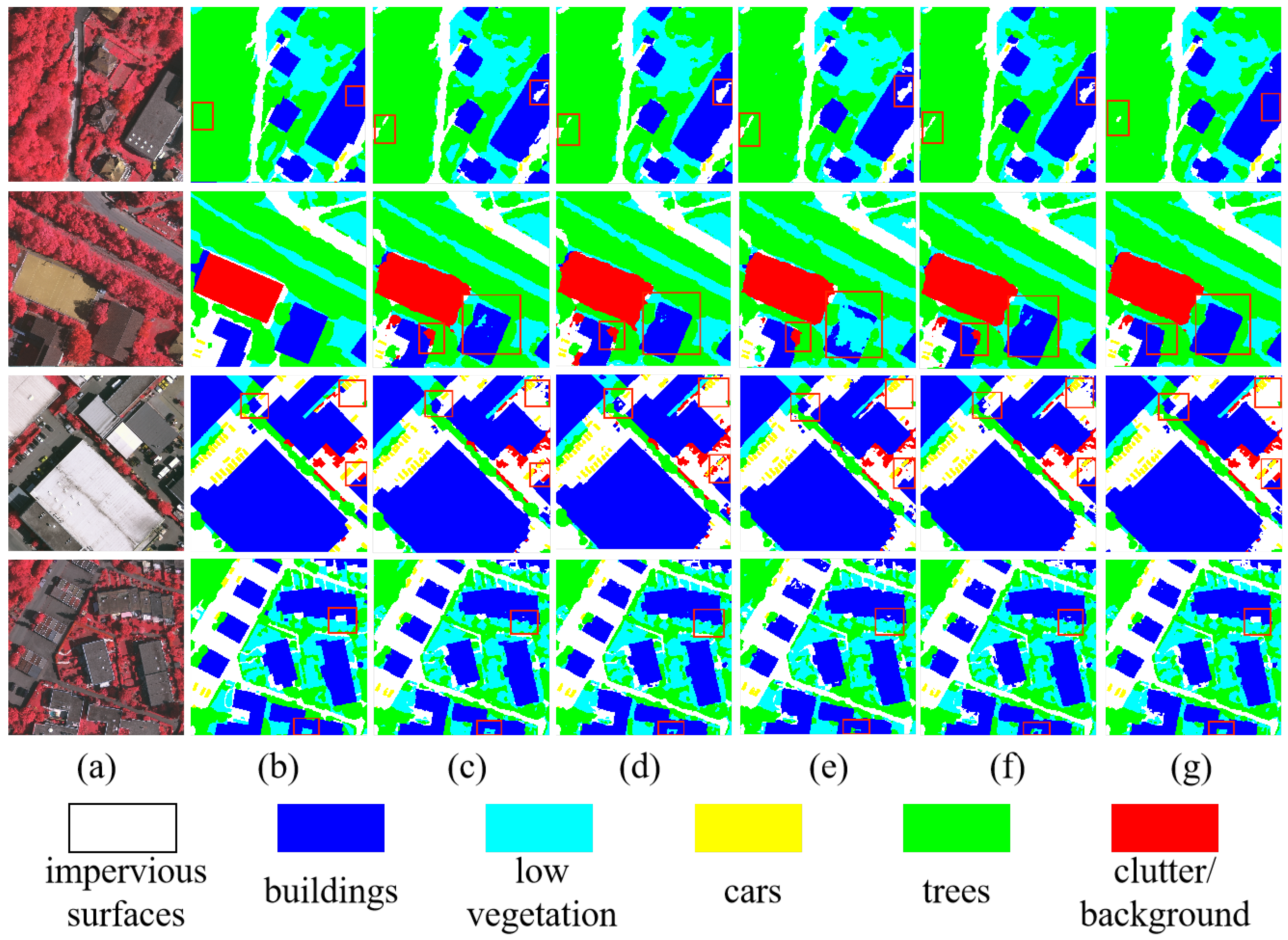
4.6.1. Results on Vaihingen

The RTMamba model, evaluated on the Vaihingen dataset using its RTMamba-s and RTMamba-b versions, showed significant advantages over current state-of-the-art (SOTA) models, as depicted in

Table 4. Comparison with state-of-the-art methods on the Vaihingen dataset. Two RTMamba versions are used for comparison: RTMamba-s and RTMamba-b. The size of the test images is $1024\times 1024$. All experiments were performed in the same environment. “↑” indicates that a higher result is preferable. The best results are in bold.

Method	Imp.surf	Building	Low.Veg	Tree	Car	Mean F1 (%) ↑	OA (%) ↑	mIoU (%) ↑
BiSeNet [9]	91.31	94.74	82.27	88.69	78.30	87.07	89.47	77.59
BiSeNetv2 [10]	91.59	94.16	82.16	89.01	78.98	87.18	89.42	77.72
DANet [39]	91.85	94.93	83.81	89.60	80.27	88.09	90.15	79.12
SCTNet-s [17]	91.31	94.02	80.45	88.56	78.14	88.25	86.50	79.46
SCTNet-b [17]	90.16	94.48	82.21	89.27	85.14	90.40	89.01	80.61
TransUNet [14]	92.80	95.40	84.40	89.90	85.30	89.50	90.70	81.30
DeeplabV3+ [7]	92.38	95.17	84.29	89.52	86.47	89.57	90.56	81.57
PSPNet [8]	92.79	95.46	84.51	89.94	88.61	90.26	90.85	82.58
UNetFormer [15]	92.70	95.30	84.90	90.60	88.50	-	-	82.70
MANet [24]	93.02	95.47	84.64	89.98	88.95	90.41	90.96	82.71
RS3Mamba * [21]	86.62	93.83	67.84	83.66	81.97	90.34	-	82.78
PIDNet [16]	92.30	95.50	85.40	89.90	89.40	-	-	83.00
RTMamba-s	92.48	94.46	85.62	90.32	85.64	89.11	90.39	81.01
RTMamba-b	93.75	95.30	85.97	90.93	88.70	91.08	91.30	83.92

* The results in the original paper.

. RTMamba-s achieved an mIoU of 81.01% at a $1024\times 1024$ resolution. In contrast to PIDNet [16], RTMamba-b showcased a performance enhancement of 0.92% in the mIoU. However, it exhibited lower segmentation accuracy for building and car objects, with mIoU scores of 0.20% and 0.70%, respectively. This was possibly influenced by various factors such as category similarity and model preferences. Additionally, compared to other models, RTMamba exhibited the most favorable performance in terms of mean F1, OA, and mIoU metrics, with scores of 91.08%, 91.30%, and 83.92%, respectively. Figure 8 presents a visual comparison of RTMamba with other SOTA methods on the Vaihingen test set, including PSPNet [8], MANet [24], SCTNet [17], and PIDNet [16]. As highlighted by the red boxes in the figure, RTMamba demonstrated superior segmentation outcomes for buildings and tree objects compared to other SOTA methods, effectively addressing issues such as boundary blur and misclassification. These results underscore the robust capability of RTMamba in remote sensing semantic segmentation tasks.

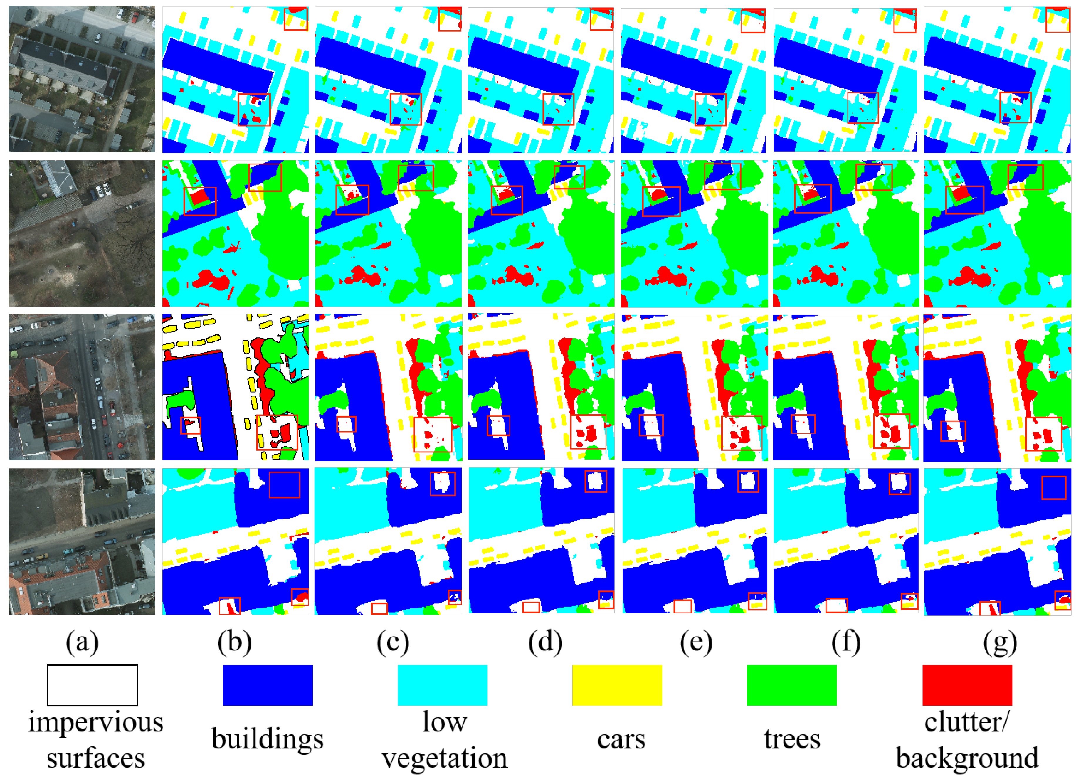
4.6.2. Results on Potsdam

Similarly, RTMamba was evaluated on the Potsdam dataset. As depicted in

Table 5. Comparison with state-of-the-art methods on the Potsdam dataset. Two RTMamba versions are used for comparison: RTMamba-s and RTMamba-b. The size of the test images is $1024\times 1024$. All experiments were performed in the same environment. “↑” indicates that a higher result is preferable. The best results are in bold.

Method	Imp.surf	Building	Low.Veg	Tree	Car	Mean F1 (%) ↑	OA (%) ↑	mIoU (%) ↑
SegNet [23]	89.83	93.27	84.62	84.37	92.51	88.92	87.21	80.26
SCTNet-s [17]	88.41	94.31	81.47	78.25	90.06	89.54	88.52	81.87
BiSeNet [9]	91.07	95.12	85.81	86.63	91.37	90.00	89.06	81.99
BiSeNetv2 [10]	90.92	94.92	85.99	86.17	91.93	89.99	89.98	81.97
SCTNet-b [17]	88.95	94.68	80.71	80.01	92.33	88.23	89.77	83.25
DeepLabV3+ [7]	92.95	95.88	87.62	88.15	96.02	92.12	90.88	84.32
DANet [39]	92.31	96.21	86.82	88.14	94.85	91.67	90.23	84.83
PSPNet [8]	93.36	96.97	87.75	88.50	95.42	92.40	91.08	84.88
TransUNet [14]	92.60	96.00	86.80	87.90	95.30	91.70	90.10	84.90
UNetFormer [15]	93.60	97.20	87.70	88.90	96.50	-	-	86.80
PIDNet [16]	92.60	96.90	89.00	89.20	96.30	-	-	86.90
MANet [24]	93.40	96.96	88.32	89.36	96.48	92.90	91.32	86.95
RTMamba-s	92.11	96.26	86.92	88.94	95.67	91.35	90.45	84.58
RTMamba-b	93.91	96.52	88.98	89.98	96.64	92.86	91.56	87.15

, comparisons were conducted with current SOTA models. The experimental results demonstrate the notable advantages of RTMamba-b over existing SOTA methods. With an input size of $1024\times 1024$, RTMamba-s achieved an mIoU score of 84.58%, surpassing the capabilities of most existing models (e.g., SCTNet-b [17]: 83.25%; DeepLabV3+ [7]: 84.32%). Specifically, RTMamba-b achieved an mIoU of 87.15%, representing a 0.2% performance improvement over MANet [24]. Additionally, compared to other models, RTMamba-b also achieved competitive results in other metrics. Figure 9 presents a visual comparison of RTMamba with other methods on the Potsdam test set. The comparison methods include PSPNet [8], MANet [24], SCTNet [17], and PIDNet [16]. The red boxes in the first and fourth rows demonstrate RTMamba’s advantage in segmenting boundary regions and achieving accurate segmentation results. The red boxes in the second and third rows illustrate that RTMamba achieved more precise segmentation results at the junctions of two different categories of objects, indicating the beneficial effect of multiscale feature interaction from the ITP module and the AFE method. Overall, RTMamba has the potential to be a valuable tool for applications in the field of remote sensing segmentation, offering a novel solution for semantic segmentation tasks in remote sensing images.

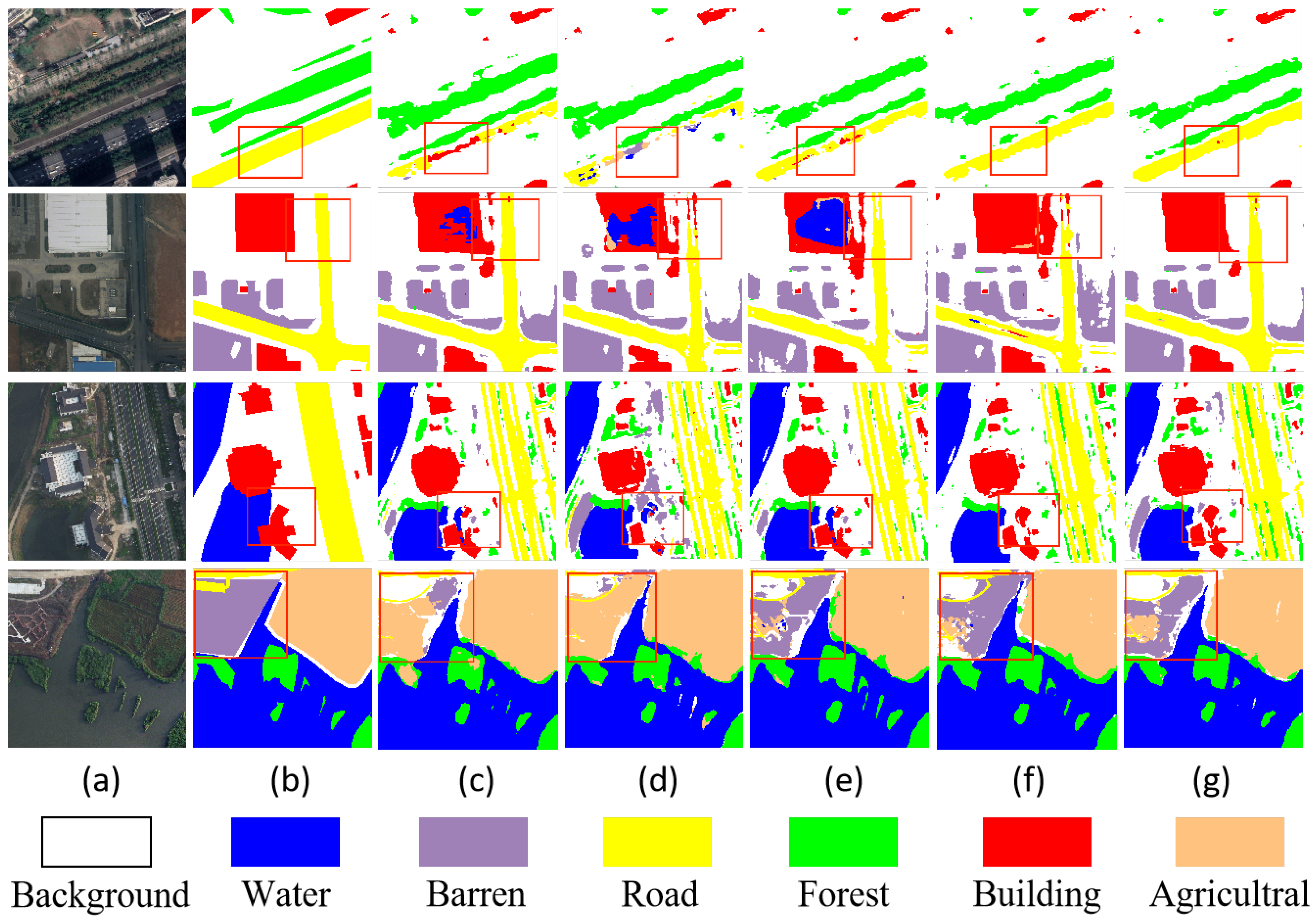
4.6.3. Results on LoveDA

We conducted an evaluation of RTMamba on the LoveDA dataset. As depicted in

Table 6. Comparison of methods on the LoveDA dataset. Two RTMamba versions are used for comparison: RTMamba-s and RTMamba-b. The test image size is $1024\times 1024$. All experiments were performed in the same environment. “↑” indicates that a higher result is preferable. The best results are in bold.

Method	Background	Building	Road	Water	Barren	Forest	Agriculture	mIoU (%) ↑	FPS ↑
SCTNet-s [17]	38.17	49.06	51.06	75.70	18.50	42.19	54.44	47.02	-
BiSeNet [9]	41.78	50.23	52.54	74.93	14.05	41.99	56.12	47.37	121.9
DeeplabV3+ [7]	42.97	50.88	52.02	74.36	10.40	44.21	58.53	47.62	53.7
SCTNet-b [17]	43.37	52.17	50.51	75.71	18.15	43.21	52.97	47.73	-
PSPNet [8]	44.40	52.13	53.52	76.50	9.73	44.07	57.85	48.31	-
BiSeNetv2 [10]	43.04	51.19	52.77	75.93	14.99	43.66	60.65	48.89	40.3
TransUNet [14]	43.00	56.10	53.70	78.00	9.30	44.90	56.90	48.90	13.4
MANet [24]	43.29	55.35	56.20	74.18	14.28	42.85	58.62	49.26	-
PIDNet [16]	44.15	54.72	56.54	76.81	17.49	47.13	57.54	50.63	52.2
RS3Mamba * [21]	39.72	58.75	57.92	61.00	37.24	39.67	33.98	50.93	-
UNetFormer [15]	44.70	58.80	54.90	79.60	20.10	46.00	62.40	52.40	115.3
RTMamba-s	42.40	51.06	50.45	76.09	18.25	43.81	58.51	48.65	139
RTMamba-b	44.72	56.43	52.49	79.90	20.96	44.46	55.06	50.57	95.63

* The results in the original paper.

, comparisons were made with current advanced models. Specifically, RTMamba-s achieved a frame rate of 139 FPS, demonstrating excellent real-time performance. Additionally, RTMamba-b outperformed most models in terms of the mIoU metric. In comparison to RS3Mamba [21], which also employs the Mamba architecture, RTMamba exhibited superior performance in the background, water, forest, and agriculture categories, with mIoU scores of 44.72%, 79.90%, 44.46%, and 55.06%, respectively. However, in the building, road, and barren categories, it lagged behind RS3Mamba. The discrepancy in the results can be attributed to the differing architectural approaches employed by RTMamba and RS3Mamba. RTMamba employs a single-branch architecture for the backbone and decoder during inference, whereas RS3Mamba employs a dual-branch architecture. This architectural divergence influenced the segmentation accuracy for different classes. Although the mIoU of UNetFormer [15] was higher than that of RTMamba-b, it lagged behind RTMamba-b for individual classes such as water, barren, and background. Figure 10 presents a visual comparison of RTMamba with other SOTA methods on the LoveDA test set, including PSPNet [8], MANet [24], SCTNet [17], and PIDNet [16]. The red boxes in the first and second lines demonstrate that RTMamba exhibited good performance in the segmentation of the road category. In the third row of images, the original image contains a substantial amount of intricate content, resulting in more intricate segmentation outcomes across numerous methodologies. In comparison, RTMamba achieved effective segmentation. In the fourth row of images, the original category in the red box is barren, but both RTMamba and other methods produced a number of incorrect segmentations. This indicates confusion between the agricultural category and the barren category, suggesting that there is still room for improvement in the existing segmentation methods. The experimental results indicate that RTMamba demonstrated competitive performance, achieving a balance between accuracy and efficiency.

5. Discussion

This paper introduces RTMamba, a real-time remote sensing segmentation framework based on a Mamba network architecture. The complex scenes in remote sensing images often lead to challenges such as noise and feature redundancy in feature extraction. This work explores the potential of SSMs in real-time segmentation tasks in remote sensing, addressing the limitations of the CNN and transformer models. RTMamba aims to effectively address these challenges. The following analysis is provided to demonstrate the effectiveness of the proposed method:

(1) Real-time capability of the model: RTMamba incorporates VSS blocks into the backbone as a method for deep feature extraction. Utilizing the 2D selection scanning algorithm effectively captures long-range dependencies while maintaining linear complexity, thereby providing a prerequisite guarantee for the real-time performance of the model. Real-time segmentation tests on the Jetson AGX Orin edge device (Figure 11) confirm RTMamba’s excellent performance (

Table 7. Real-world performance of RTMamba-s/b on Jetson AGX Orin, evaluated using various input sizes and acceleration methods (e.g., TensorRT, ONNX). “↑” indicates that a higher result is preferable. “↓” indicates that a lower result is preferable.

Method	Inference	Acceleration	Data Type	Latency ↓	FPS ↑
RTMamba-s	$512\times 512$	ONNX	fp32	16.736	59.751
RTMamba-s	$512\times 512$	TensorRT	fp16	16.334	61.222
RTMamba-s	$512\times 1024$	ONNX	fp32	19.482	51.329
RTMamba-s	$512\times 1024$	TensorRT	fp16	17.881	55.927
RTMamba-s	$1024\times 1024$	ONNX	fp32	22.846	43.771
RTMamba-s	$1024\times 1024$	TensorRT	fp16	20.825	48.018
RTMamba-b	$512\times 512$	ONNX	fp32	17.400	57.472
RTMamba-b	$512\times 512$	TensorRT	fp16	16.224	61.638
RTMamba-b	$512\times 1024$	ONNX	fp32	19.055	52.479
RTMamba-b	$512\times 1024$	TensorRT	fp16	18.753	53.324
RTMamba-b	$1024\times 1024$	ONNX	fp32	22.446	44.551
RTMamba-b	$1024\times 1024$	TensorRT	fp16	21.570	46.360

). Using multiscale input inference with TensorRT [40] and ONNX [41], RTMamba achieves speeds exceeding 43 FPS. Additionally, the lightweight RTMamba-s model, comprising only 5.82M parameters, sets the stage for future deployment on UAVs.

(2) Addressing the challenges posed by noise and feature redundancy: The ITP module, located within the decoder, effectively filters redundant information. It employs a multiscale pooling strategy using different pooling operation sizes. This enables feature maps to capture varying receptive-field sizes, leading to a more comprehensive characterization of the information present in the image. Subsequently, partial convolution (PConv) reduces redundant computations and memory accesses, facilitating efficient spatial feature extraction. The adaptive feature enhancement (AFE) operation within the inverted triangular structure is designed to focus on important information, consequently leading to refined segmentation results. To elucidate the role of the ITP module, we leverage GradCAM [42] to generate attention heatmaps for different classes on the LoveDA test set (Figure 12). Each column in the figure represents a visualization of attention for a specific class, namely (a) building, (b) road, (c) water, (d) barren, (e) forest, and (f) agriculture. Six remote sensing images from the test set are displayed in the first row. The second and third rows present visualizations of attention levels for corresponding class objects before and after ITP processing, respectively. Darker colors indicate a higher level of attention at that position. The comparison clearly demonstrates that after ITP processing, the model focuses more on regions corresponding to each class. This illustrates AFE’s ability to enhance the model’s responsiveness to specific information, thereby facilitating the generation of refined segmentation results.

(3) Lightweight nature of the model: During the training phase, RTMamba undergoes joint training with the semantic transformer. Through alignment loss, it effectively aligns the feature distribution with the transformer. During the inference phase, only the backbone and decoder parts are retained, which does not affect the inference performance. This ensures the lightweight nature of the model.

The effectiveness of RTMamba is demonstrated through ablative and comparative experiments, showcasing its competitive object segmentation performance in aerial remote sensing images. Particularly, RTMamba achieves superior results on the Vaihingen and Potsdam datasets and maintains a balanced speed–accuracy tradeoff on the LoveDA dataset.

Additionally, this article acknowledges certain limitations. Firstly, concerning the application of SSMs, we did not delve into exploring the effectiveness of further designing any variants. Based on the current experimental results, RTMamba emerges as an excellent method suitable for real-time remote sensing segmentation. Secondly, regarding the dataset experiments, we conducted validation using three aerial remote sensing datasets. However, further validation in real-world situations is still required. Lastly, it is important to note that RTMamba is presently tailored for single RGB modalities, thus limiting its applicability to multi-modal data. Moving forward, we intend to persist in exploring real-time segmentation on actual UAV devices, alongside further investigation into multi-modal real-time remote sensing segmentation tasks.

6. Conclusions

This paper introduces RTMamba, a novel architecture tailored for real-time remote sensing segmentation tasks, particularly for resource-constrained embedded devices like UAVs. The backbone integrates VSS blocks to effectively capture long-range dependencies with linear computational complexity. Additionally, a novel ITP module within the decoder suppresses noise, filters redundant information, and enhances object perception in remote sensing images at reduced computational cost. During training, the semantic transformer enriches the backbone and decoder with semantic and spatial details. Comparative experiments on three aerial datasets demonstrate RTMamba’s superior performance on the Vaihingen and Potsdam datasets and a balanced accuracy–speed tradeoff on the LoveDA dataset. Speed tests on the Jetson AGX Orin edge device confirm RTMamba’s excellent real-time performance, highlighting its potential for UAV deployment.

It should be noted that the proposed method also has certain limitations. Firstly, due to the differences in floating-point precision between edge devices and GPU devices, there is a certain performance loss when testing on edge devices. Further optimization is needed to reduce this loss. Secondly, in the visual representation of the segmentation results on the LoveDA dataset, our method exhibits issues such as classification errors, missing segmentation regions, and blurry edge segmentation. Therefore, RTMamba still has room for improvement, such as designing a lightweight edge feature extraction module and applying novel loss functions. Finally, our method is not yet sufficiently developed for practical application in drones and requires extensive experimental testing to verify its stability and reliability in various complex environments.

In future work, we will continue to conduct segmentation experiments with RTMamba on real drone devices and study the application of multi-modal Mamba semantic segmentation methods.

References

1. Talukdar, S.; Singha, P.; Mahato, S.; Pal, S.; Liou, Y.A.; Rahman, A. Land-use land-cover classification by machine learning classifiers for satellite observations—A review. Remote Sens. 2020, 12, 1135. [Google Scholar] [CrossRef]
2. Phan, T.N.; Kuch, V.; Lehnert, L.W. Land cover classification using Google Earth Engine and random forest classifier—The role of image composition. Remote Sens. 2020, 12, 2411. [Google Scholar] [CrossRef]
3. Krizhevsky, A.; Sutskever, I.; Hinton, G.E. Imagenet classification with deep convolutional neural networks. Adv. Neural Inf. Process. Syst. 2012, 25, 84–90. [Google Scholar] [CrossRef]
4. Grinias, I.; Panagiotakis, C.; Tziritas, G. MRF-based segmentation and unsupervised classification for building and road detection in peri-urban areas of high-resolution satellite images. ISPRS J. Photogramm. Remote Sens. 2016, 122, 145–166. [Google Scholar] [CrossRef]
5. Long, J.; Shelhamer, E.; Darrell, T. Fully convolutional networks for semantic segmentation. In Proceedings of the IEEE Conference on Computer Vision and Pattern Recognition (CVPR), Boston, MA, USA, 7–12 June 2015; pp. 3431–3440. [Google Scholar]
6. Ronneberger, O.; Fischer, P.; Brox, T. U-net: Convolutional networks for biomedical image segmentation. In Proceedings of the Medical Image Computing and Computer-Assisted Intervention–MICCAI 2015: 18th International Conference (Part III 18), Munich, Germany, 5–9 October 2015; Springer: Berlin/Heidelberg, Germany, 2015; pp. 234–241. [Google Scholar]
7. Chen, L.C.; Zhu, Y.; Papandreou, G.; Schroff, F.; Adam, H. Encoder-decoder with atrous separable convolution for semantic image segmentation. In Proceedings of the European Conference on Computer Vision (ECCV), Munich, Germany, 8–14 September 2018; pp. 801–818. [Google Scholar]
8. Zhao, H.; Shi, J.; Qi, X.; Wang, X.; Jia, J. Pyramid scene parsing network. In Proceedings of the IEEE Conference on Computer Vision and Pattern Recognition (CVPR), Honolulu, HI, USA, 21–26 July 2017; pp. 2881–2890. [Google Scholar]
9. Yu, C.; Wang, J.; Peg, C.; Gao, C.; Yu, G.; Sang, N. Bisenet: Bilateral segmentation network for real-time semantic segmentation. In Proceedings of the European Conference on Computer Vision (ECCV), Munich, Germany, 8–14 September 2018; pp. 325–341. [Google Scholar]
10. Yu, C.; Gao, C.; Wang, J.; Yu, G.; Shen, C.; Sang, N. Bisenet v2: Bilateral network with guided aggregation for real-time semantic segmentation. Int. J. Comput. Vis. 2021, 129, 3051–3068. [Google Scholar] [CrossRef]
11. Zhou, W.; Fan, X.; Yan, W.; Shan, S.; Jiang, Q.; Hwang, J.N. Graph attention guidance network with knowledge distillation for semantic segmentation of remote sensing images. IEEE Trans. Geosci. Remote Sens. 2023, 61, 4506015. [Google Scholar] [CrossRef]
12. Hong, Y.; Pan, H.; Sun, W.; Jia, Y. Deep dual-resolution networks for real-time and accurate semantic segmentation of road scenes. arXiv 2021, arXiv:2022.3228042. [Google Scholar]
13. Shi, W.; Meng, Q.; Zhang, L.; Zhao, M.; Su, C.; Jancsó, T. DSANet: A deep supervision-based simple attention network for efficient semantic segmentation in remote sensing imagery. Remote Sens. 2022, 14, 5399. [Google Scholar] [CrossRef]
14. Chen, J.; Lu, Y.; Yu, Q.; Luo, X.; Adeli, E.; Wang, Y.; Lu, L.; Yuille, A.L.; Zhou, Y. Transunet: Transformers make strong encoders for medical image segmentation. arXiv 2021, arXiv:2102.04306. [Google Scholar]
15. Wang, L.; Li, R.; Zhang, C.; Fang, S.; Duan, C.; Meng, X.; Atkinson, P.M. UNetFormer: A UNet-like transformer for efficient semantic segmentation of remote sensing urban scene imagery. ISPRS J. Photogramm. Remote Sens. 2022, 190, 196–214. [Google Scholar] [CrossRef]
16. Xu, J.; Xiong, Z.; Bhattacharyya, S.P. PIDNet: A real-time semantic segmentation network inspired by PID controllers. In Proceedings of the IEEE/CVF Conference on Computer Vision and Pattern Recognition (CVPR), Vancouver, BC, Canada, 17–24 June 2023; pp. 19529–19539. [Google Scholar]
17. Xu, Z.; Wu, D.; Yu, C.; Chu, X.; Sang, N.; Gao, C. SCTNet: Single-Branch CNN with Transformer Semantic Information for Real-Time Segmentation. Proc. Aaai Conf. Artif. Intell. 2024, 38, 6378–6386. [Google Scholar] [CrossRef]
18. Gu, A.; Dao, T. Mamba: Linear-time sequence modeling with selective state spaces. arXiv 2023, arXiv:2312.00752. [Google Scholar]
19. Chen, K.; Chen, B.; Liu, C.; Li, W.; Zou, Z.; Shi, Z. Rsmamba: Remote sensing image classification with state space model. arXiv 2024, arXiv:2403.19654. [Google Scholar] [CrossRef]
20. Zhao, S.; Chen, H.; Zhang, X.; Xiao, P.; Bai, L.; Ouyang, W. Rs-mamba for large remote sensing image dense prediction. arXiv 2024, arXiv:2404.02668. [Google Scholar] [CrossRef]
21. Ma, X.; Zhang, X.; Pun, M.O. RS3Mamba: Visual State Space Model for Remote Sensing Images Semantic Segmentation. arXiv 2024, arXiv:2404.02457. [Google Scholar] [CrossRef]
22. Barnell, M.; Raymond, C.; Smiley, S.; Isereau, D.; Brown, D. Ultra low-power deep learning applications at the edge with Jetson Orin AGX hardware. In Proceedings of the 2022 IEEE High Performance Extreme Computing Conference (HPEC), Waltham, MA, USA, 19–23 September 2022; pp. 1–4. [Google Scholar]
23. Badrinarayanan, V.; Kendall, A.; Cipolla, R. Segnet: A deep convolutional encoder-decoder architecture for image segmentation. IEEE Trans. Pattern Anal. Mach. Intell. 2017, 39, 2481–2495. [Google Scholar] [CrossRef] [PubMed]
24. Chen, B.; Xia, M.; Qian, M.; Huang, J. MANet: A multi-level aggregation network for semantic segmentation of high-resolution remote sensing images. Int. J. Remote Sens. 2022, 43, 5874–5894. [Google Scholar] [CrossRef]
25. He, W.; Han, K.; Tang, Y.; Wang, C.; Yang, Y.; Guo, T.; Wang, Y. Densemamba: State space models with dense hidden connection for efficient large language models. arXiv 2024, arXiv:2403.00818. [Google Scholar]
26. Zhu, L.; Liao, B.; Zhang, Q.; Wang, X.; Liu, W.; Wang, X. Vision mamba: Efficient visual representation learning with bidirectional state space model. arXiv 2024, arXiv:2401.09417. [Google Scholar]
27. Liu, Y.; Tian, Y.; Zhao, Y.; Yu, H.; Xie, L.; Wang, Y.; Ye, Q.; Liu, Y. Vmamba: Visual state space model. arXiv 2024, arXiv:2401.10166. [Google Scholar]
28. Zhang, Z.; Liu, A.; Reid, I.; Hartley, R.; Zhuang, B.; Tang, H. Motion mamba: Efficient and long sequence motion generation with hierarchical and bidirectional selective ssm. arXiv 2024, arXiv:2403.07487. [Google Scholar]
29. Shu, C.; Liu, Y.; Gao, J.; Yan, Z.; Shen, C. Channel-wise knowledge distillation for dense prediction. In Proceedings of the IEEE/CVF International Conference on Computer Vision (ICCV), Montreal, QC, Canada, 10–17 October 2021; pp. 5311–5320. [Google Scholar]
30. Chen, J.; Kao, S.h.; He, H.; Zhuo, W.; Wen, S.; Lee, C.H.; Chan, S.H.G. Run, Don’t walk: Chasing higher FLOPS for faster neural networks. In Proceedings of the IEEE/CVF Conference on Computer Vision and Pattern Recognition (CVPR), Vancouver, BC, Canada, 17–24 June 2023; pp. 12021–12031. [Google Scholar]
31. Milletari, F.; Navab, N.; Ahmadi, S.A. V-net: Fully convolutional neural networks for volumetric medical image segmentation. In Proceedings of the 2016 Fourth International Conference on 3D Vision (3DV), Stanford, CA, USA, 25–28 October 2016; pp. 565–571. [Google Scholar]
32. Wang, J.; Zheng, Z.; Ma, A.; Lu, X.; Zhong, Y. LoveDA: A remote sensing land-cover dataset for domain adaptive semantic segmentation. arXiv 2021, arXiv:2110.08733. [Google Scholar]
33. 2D Semantic Labeling Contest—Vaihingen. Available online: https://www.isprs.org/education/benchmarks/UrbanSemLab/2d-semlabel-vaihingen.aspx (accessed on 8 February 2022).
34. 2D Semantic Labeling Contest—Potsdam. Available online: https://www.isprs.org/education/benchmarks/UrbanSemLab/2d-semlabel-potsdam.aspx (accessed on 8 February 2022).
35. Xie, E.; Wang, W.; Yu, Z.; Anandkumar, A.; Alvarez, J.M.; Luo, P. SegFormer: Simple and efficient design for semantic segmentation with transformers. Adv. Neural Inf. Process. Syst. 2021, 34, 12077–12090. [Google Scholar]
36. Zhang, R.; Zhang, Q.; Zhang, G. LSRFormer: Efficient Transformer Supply Convolutional Neural Networks with Global Information for Aerial Image Segmentation. IEEE Trans. Geosci. Remote Sens. 2024, 62, 5610713. [Google Scholar] [CrossRef]
37. Loshchilov, I.; Hutter, F. Decoupled weight decay regularization. arXiv 2017, arXiv:1711.05101. [Google Scholar]
38. Contributors, M. MMSegmentation: OpenMMLab Semantic Segmentation Toolbox and Benchmark. 2020. Available online: https://github.com/open-mmlab/mmsegmentation (accessed on 8 February 2022).
39. Xue, H.; Liu, C.; Wan, F.; Jiao, J.; Ji, X.; Ye, Q. Danet: Divergent activation for weakly supervised object localization. In Proceedings of the IEEE/CVF International Conference on Computer Vision (ICCV), Seoul, Republic of Korea, 27 October–2 November 2019; pp. 6589–6598. [Google Scholar]
40. Jeong, E.; Kim, J.; Tan, S.; Lee, J.; Ha, S. Deep learning inference parallelization on heterogeneous processors with tensorrt. IEEE Embed. Syst. Lett. 2021, 14, 15–18. [Google Scholar] [CrossRef]
41. Jajal, P.; Jiang, W.; Tewari, A.; Woo, J.; Thiruvathukal, G.K.; Davis, J.C. Analysis of failures and risks in deep learning model converters: A case study in the onnx ecosystem. arXiv 2023, arXiv:2303.17708. [Google Scholar]
42. Selvaraju, R.R.; Cogswell, M.; Das, A.; Vedantam, R.; Parikh, D.; Batra, D. Grad-cam: Visual explanations from deep networks via gradient-based localization. In Proceedings of the IEEE/CVF International Conference on Computer Vision (ICCV), Venice, Italy, 22–29 October 2017; pp. 618–626. [Google Scholar]
Figure 1. Overview of the proposed RTMamba. The backbone employs VSS blocks for feature extraction, while the decoder integrates the ITP module to filter redundant feature information. During training, the semantic transformer blocks, indicated in gray, provide semantic and spatial detail information to the backbone.
Remotesensing 16 02620 g001
Figure 2. Detailed depiction of the VSS block, where SS2D denotes the 2D selective scanning operation.
Remotesensing 16 02620 g002
Figure 3. 2D selective scanning (SS2D) process. It mainly consists of three operations, namely a scan expanding operation, an S6 operation, and a scan merging operation.
Remotesensing 16 02620 g003
Figure 4. Design of ITP module. PConv is the partial convolution operation. AFE is the adaptive feature fusion module.
Remotesensing 16 02620 g004
Figure 5. Visual analysis of ablation experiments on components on the Vaihingen and Potsdam datasets.
Remotesensing 16 02620 g005
Figure 6. Different designs of the ITP module. (a) Additive feature fusion (AFF); (b) Multiplicative feature fusion (MFF); (c) Adaptive Feature Enhancement (AFE).
Remotesensing 16 02620 g006
Figure 7. Ablation experiments on the d-state value in the VSS block on the Vaihingen test set. The five figures correspond to the mean F1, OA, mIoU, FPS, and Params values on the Vaihingen test set.
Remotesensing 16 02620 g007
Figure 8. Visual representation of segmentation results on the Vaihingen test set using multiple lightweight models. The size of the segmentation image is 1024 × 1024. (a) Input; (b) Ground truth; (c) PSPNet; (d) MANet; (e) SCTNet; (f) PIDNet; (g) RTMamba (ours).
Remotesensing 16 02620 g008
Figure 9. Visual comparison of segmentation results on the Potsdam test set using multiple lightweight models. The size of the segmentation image is 1024 × 1024 . (a) Input; (b) Ground truth; (c) PSPNet; (d) MANet; (e) SCTNet; (f) PIDNet; (g) RTMamba (ours).
Remotesensing 16 02620 g009
Figure 10. Visual representation of segmentation results on the LoveDA test set using multiple lightweight models. The size of the segmentation image is 1024 × 1024 . (a) Input; (b) Ground truth; (c) PSPNet; (d) MANet; (e) SCTNet; (f) PIDNet; (g) RTMamba (ours).
Remotesensing 16 02620 g010
Figure 11. Jetson AGX Orin edge device.
Remotesensing 16 02620 g011
Figure 12. Heatmaps of attention levels for different classes using the ITP module on the LoveDA test set. (a) Building; (b) Road; (c) Water; (d) Barren; (e) Forest; (f) Agriculture.
Remotesensing 16 02620 g012