Article

Improved ISAL Imaging Based on RD Algorithm and Image Translation Network Cascade

1
Changchun Institute of Optics, Fine Mechanics and Physics, Chinese Academy of Sciences, Changchun 130024, China
2
University of Chinese Academy of Sciences, Beijing 100049, China
3
Key Laboratory for Applied Statistics of MOE, School of Mathematics and Statistics, Northeast Normal University, Changchun 130024, China
*
Author to whom correspondence should be addressed.
These authors contributed equally to the work.
Remote Sens. 2024, 16(14), 2635; https://doi.org/10.3390/rs16142635
Submission received: 2 July 2024 / Revised: 14 July 2024 / Accepted: 16 July 2024 / Published: 18 July 2024
(This article belongs to the Special Issue Advances in Remote Sensing, Radar Techniques, and Their Applications)

Abstract

:
Inverse synthetic aperture LiDAR (ISAL) can create high-resolution images within a few milliseconds, which are employed for long-range airspace target identification. However, its optical signal characteristics incur the non-negligible higher-order kinematic parameters of the target and phase errors due to atmospheric turbulence. These higher-order parameters and phase errors make it challenging for imaging the ISAL signals. In this paper, we propose an approach integrating the RD algorithm with an image translation network. Unlike the conventional methods, our approach does not require high accuracy in estimating each target motion and atmospheric parameter. The phase error of the RD image is fitted by an image translation network, which greatly simplifies the computational difficulty of the ISAL imaging model. The experimental results demonstrate that our model has good generalization performance. Specifically, our method consistently performs well in capturing the target information under different types of noise and sparsity aperture (SA) rates compared to other conventional methods. In addition, our approach can be applied to the measured data after training the network by using simulated data.

1. Introduction

Inverse synthetic aperture LiDAR (ISAL) is an active imaging LiDAR technology similar to inverse synthetic aperture radar (ISAR), and it is widely used in the fields of military defense and target identification. ISAL emits signals towards a target and captures the reflected signals, operating continuously to provide all-weather coverage. The performance difference between ISAL and ISAR primarily depends on the signal wavelength. The wavelength of lasers is much shorter than microwaves [1], allowing ISAL to achieve higher-resolution imaging in a shorter period of time compared to ISAR. ISAL achieves range resolution by emitting broadband signals and azimuth resolution by synthetic aperture techniques [2], making the resolution distance-independent and overcoming the diffraction and limitations in conventional optical imaging. It can theoretically still achieve a sub-centimeter resolution at ultra-long distances.
However, due to the large bandwidth and high frequency of the laser signal, coupled with the short coherent imaging time of ISAL [3], it becomes challenging to ignore the higher-order terms of target motion. This makes the phase error caused by target motion in ISAL more complex than in ISAR. The broadband and frequency requirements of laser pulse signals are constrained by laser modulation technology, leading to random errors in the initial phase of the emitted signals. Additionally, the extra phase error induced by atmospheric turbulence further degrades the image resolution [4]. These factors collectively affect ISAL’s ability to obtain an ideal focused image.
The traditional ISAL image focusing methods usually rely on signal processing techniques [5], such as Fourier transform [6] and wavelet transform [7]. For instance, Li et al. [8] proposed a robust autofocus approach for motion compensation in the ISAR imaging of moving targets. Xing et al. [9] suggested a pre-processing algorithm to mitigate Migration of Resolution Cells (MTRCs) caused by rotational motion, ultimately producing a focused ISAR image. Zhao et al. [10] achieved a high-resolution radar image by estimating the sparse scattering coefficients and phase errors in both the individual and global stages, leveraging sparsity statistically. These methods generally depend on prior assumptions, such as the target movement following a specific statistical distribution, limiting their adaptability to the diversity and complexity of real target motions in the optical band. In recent years, new statistical methods and compensation schemes have been developed to enhance the quality of ISAL images. Wang et al. [11] proposed frequency descent (FD) minimum entropy optimization to compensate for the vibration phase errors from satellite microvibration. Xue et al. [12] used the Kirchhoff approximation and convolution back-projection algorithm to obtain ISAL images under various turbulence conditions. Li et al. [13] introduced an adaptive compensation method that handles the motion errors of maneuvering targets by estimating and compensating for various types of errors introduced during the target motion process.
In contrast, deep learning-based methods have shown advantages due to their potential to handle complex and highly noisy scenes [14,15,16,17]. For active imaging models such as ISAL, generative adversarial networks (GAN) have emerged as the most promising approach for unsupervised learning on complex distributions in recent years [18]. An attention GAN has been applied to low-sampling ISAR imaging [19], and an improved attention GAN has been utilized for ISAR imaging to enhance the performance [20]. Additionally, a sparse feature extraction method based on dilated convolution has been proposed to improve the reconstruction quality of ISAR images [21]. However, these deep learning methods primarily address the problems under microwave signals and often rely on specific imaging models to solve particular problems. As LiDAR technology advances and the demand for higher-resolution and more accurate imaging increases, there is a growing need for more powerful and efficient image restoration techniques for ISAL. These techniques must effectively handle both alternative motion compensation schemes and the elimination of the phase errors caused by atmospheric conditions.
In this paper, we propose an improved network combining the RD algorithm with the image translation network [22]. Specifically, we first use the RD algorithm to generate a roughly compensated RD image and further utilize the image translation network to learn the joint distribution of the RD image and the point-target projection image, and finally obtain a focused ISAL image. Our model incorporates a spatial attention mechanism to extract the features of ISAL images, addressing issues such as the inaccurate compensation for the radial motion of scattering points and clutter due to signal transmission. Additionally, we propose using multiple densely cascaded layers in variational autoencoders (VAEs) and generators to enhance the network performance. The main contributions of our proposed model are as follows. Firstly, the network autonomously learns the complex features of ISAL images without requiring the precise modeling of different targets in ISAL imaging. Secondly, the spatial attention module enhances the features related to the defocus of the scattering points in ISAL images, making the network more suitable for ISAL imaging. Lastly, our model can be applied to real-world airspace scenarios after training the network on simulated data with scattering points.
This paper is organized as follows. In Section 2, we introduce the imaging principle of ISAL and explain the reasons for ISAL’s unique performance in the optical band. In Section 3, we detail the RD algorithm and image translation network. In Section 4, we present our dataset and experimental results. Finally, in Section 5, we conclude the paper and outline the direction for future work.

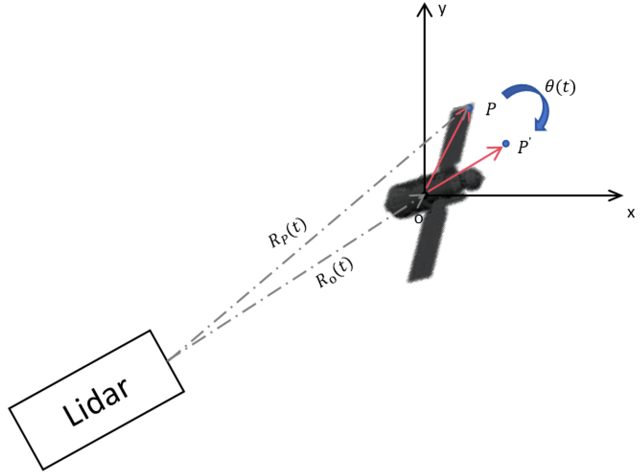
2. Signal Model of ISAL

Figure 1 illustrates the geometric model used by ISAL for imaging non-cooperative targets at long range. Point o represents the geometric center of the target, point p indicates a scattering point at the edge of the satellite, and the coordinate plane x o y represents the image planes of the target. The relative motion between the LiDAR and the target in ISAL imaging can be divided into translational component and rotational components. The distance from the LiDAR to point p is provided by Equation (1):
R p ( t ) = R o ( t ) + x p s i n ( θ ( t ) ) y p c o s ( θ ( t ) )
where R o ( t ) and θ ( t ) are the distance of the LiDAR to the o point and the rotation angle p o p , respectively. And
R o ( t ) = R 0 + v t + 1 2 a t 2 , θ ( t ) = ω t + 1 2 τ t 2 ,
where R 0 is the target’s initial displacement, and v, a, ω , and τ represent velocity, acceleration, angular velocity, and angular acceleration of the target, respectively. Since the coherent processing interval (CPI) of the ISAL is extremely short, the distance R p ( t ) can be approximated by
R p ( t ) = R o ( t ) + v t + 1 2 a t 2 + x p θ ( t ) y p .
Typically, ISAL uses linear frequency modulation (LFM) signals for target detection [23]. These signals satisfy the conditions for pulse compression and can be expressed as
L ( t f , t s ) = r e c t ( t f T a ) · e x p ( j 2 π ( f c t + 1 2 K r t f 2 ) )
where the rectangle function
r e c t ( x ) = 1 , x 1 2 0 , x > 1 2 ,
and f c and T a are the carrier frequency and pulse width, respectively. The ratio K r = B / T a represents the frequency modulation rate, where B is the bandwidth of LFM signal. The slow time t s = t t f = s · P R I , where s is the number of transmitted pulses, P R I represents the pulse repetition interval, and t and t f are full time and fast time, respectively.
The signal is reflected by the target and received by the LiDAR. Considering Equations (3) and (4), the sum of echo signals for the scatter points is provided by
L r ( t f , t s ) p A p r e c t ( t f 2 R p ( t ) / c T a ) · e x p ( j 2 π ( f c ( t 2 R p ( t ) / c ) ) · e x p ( j π K r ( t f 2 R p ( t ) / c ) 2 )
where c is the light speed and A p is the scattering coefficient at point p. To modulate the signal, we adopt the de-chirp modulation technique. It uses a time-fixed LFM signal as a reference signal and processes the differential frequency for the echo signal [24]. The reference signal can be written as
L r e f ( t f , t s ) r e c t ( t f 2 R r e f / c T r e f ) r e c t ( t s T c ) · e x p ( j 2 π ( f c ( t 2 R r e f / c ) ) · e x p ( j π K r ( t f 2 R r e f / c ) 2 )
where R r e f and T r e f are the reference distance and reference pulse width, respectively. The carrier frequency of the reference signal is the same as that of the transmitter signal, and, in the ISAL system, we have that T a T r e f . At this point, we can obtain the echo signal S ( t f , t s ) after de-chirp modulation:
S ( t f , t s ) = L r ( t f , t s ) · L r e f * ( t f , t s ) p A p r e c t ( t f 2 R p ( t ) / c T a ) r e c t ( t s T c ) e x p [ j ( φ ( t f , t s ) + φ 0 ) ] .
This two-dimensional matrix signal S ( t f , t s ) is received by the LiDAR after the coherent detection, consisting of the number of distance gates and the number of pulses. The phase error φ ( t f , t s ) can be computed by
φ ( t f , t s ) = 4 π ( f c τ t + K r τ t ( t f t r e ) K r τ t 2 )
where τ t is the delay time, equal to R p R r e f / c , and t r e is the delay time of the local oscillator light field, equal to 2 R r e f / c . Equation (8) provides the motion information of the target. The range profile of signal can be expressed as
S ( f f , t s ) = F S ( t f , t s ) t f = p A p T a · s i n c ( T a ( f f + 2 K r τ t ) ) · r e c t ( t s T c ) · e x p ( j 4 π f f τ t ) · e x p ( j 4 π ( f c τ t + K r τ t 2 ) ) · e x p ( j φ 0 ) .
The above model is similar to the ISAR system. However, optical signals in ISAL have significantly higher carrier frequencies and bandwidths compared to microwave signals. As a result, the target does not satisfy the uniform motion at the time of the each pulse, making it more challenging to estimate the delay time τ t in the ISAL than the ISAR. Those factors make the "one-step-and-stop" model used in ISAR [25] does not apply to ISAL and traditional methods lead to defocusing issues in ISAL imaging. In addition, the laser wavelength is highly sensitive to atmospheric interference during transmission, leading to dramatic variations in the resulting image phase error φ 0 . These factors all make the ISAL image blurred.

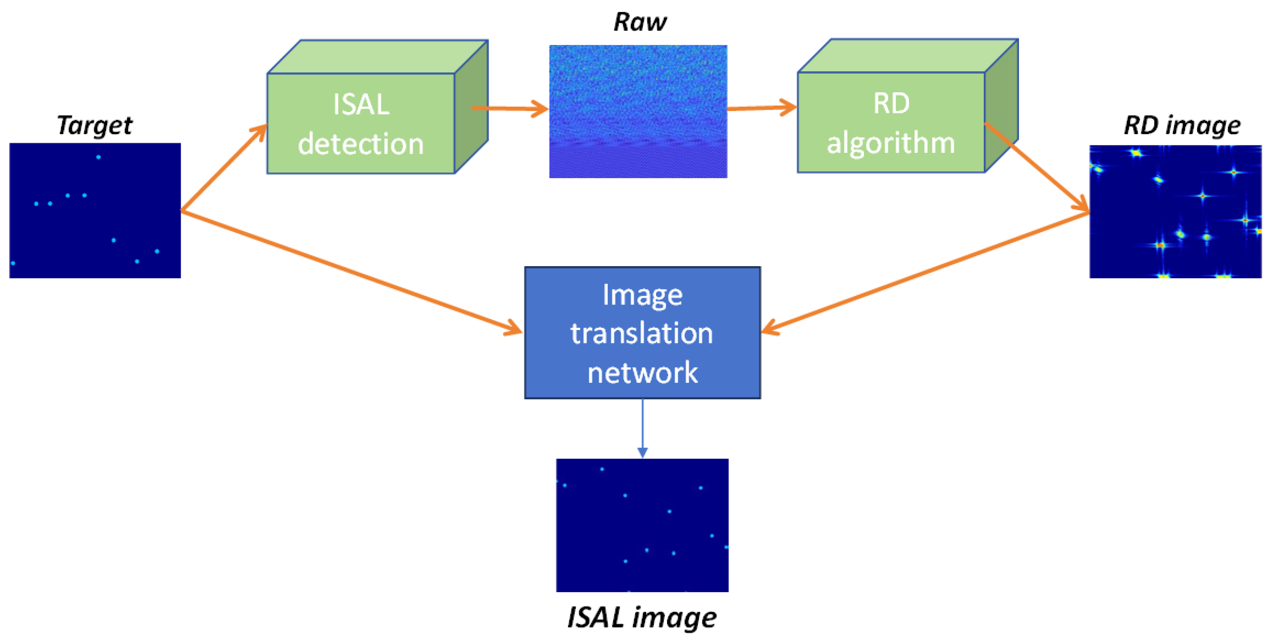
3. Structure of Proposed Network

To mitigate the impact of the phase error in Equation (9) on the ISAL imaging, we design a structure that cascades an RD algorithm with an image translation network, shown in Figure 2. Initially, our method utilizes the RD algorithm to obtain an ISAL image, which provides rough compensation for phase errors resulting from target motion. Subsequently, an image translation network addresses issues such as envelope drift and Migration of MTRCs, which arise from inaccuracies in the compensation of the RD algorithm. Furthermore, this network eliminates phase error induced by atmospheric influences during signal transmission, ultimately enhancing the quality ISAL image.

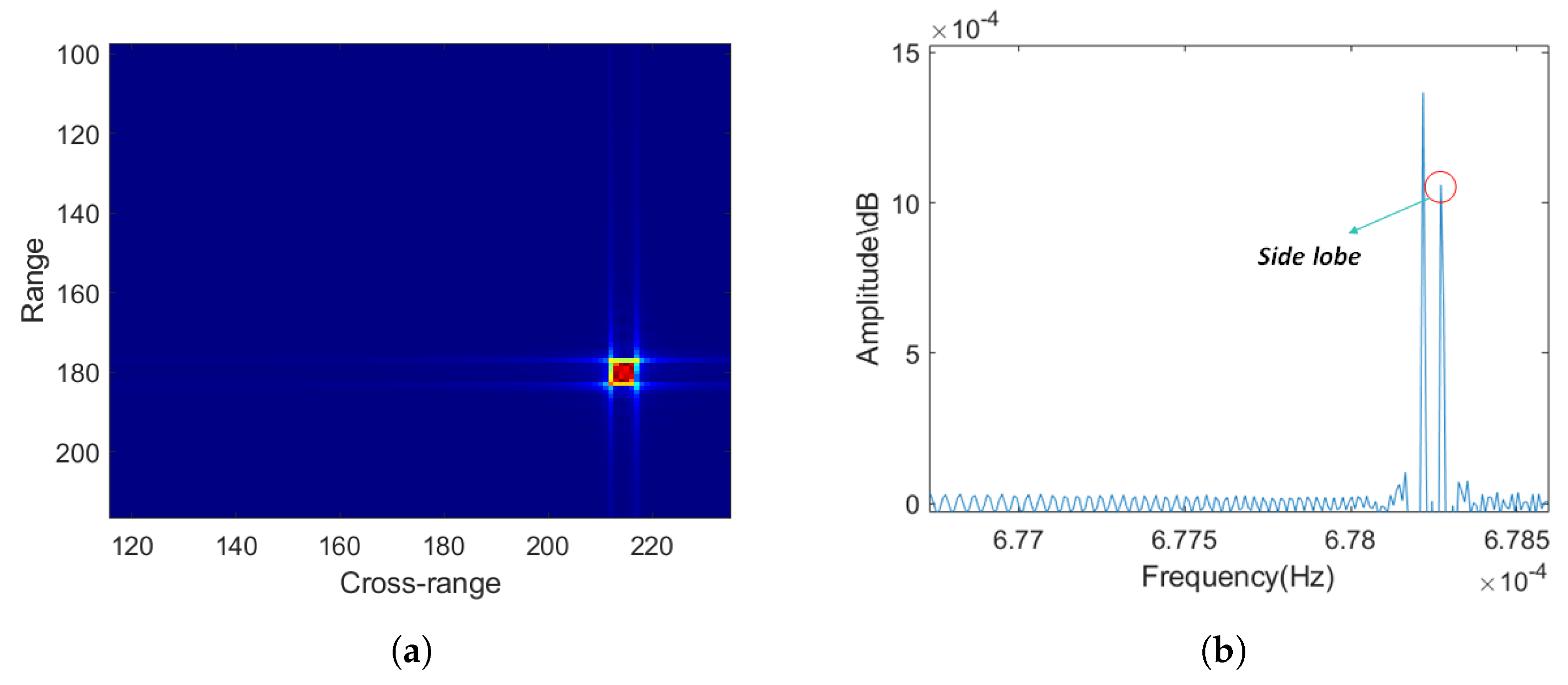
3.1. Range-Doppler Algorithm

The RD algorithm obtains ISAL images by separating the range and azimuth directions of the target for compensation. Initially, the target could approximate to a turntable model by implementing the translation compensation, and we align the signal envelope by using the minimum entropy method in the RD algorithm. Subsequently, rotational envelope compensation is performed after estimating the rotational Doppler shift. Finally, inverse fast Fourier transform (IFFT) is applied to the transformation of the frequency domain signal, generating the ISAL image in the Range-Doppler domain. Further details are provided in Algorithm 1.
According to the signal model of ISAL, the rotational error of ISAL affects the accuracy of translational compensation, and the residual error of translational compensation prevents the rotational error from being fully corrected [3]. As shown in Figure 3, envelope drift persists in the range direction even after incompletely compensating for translational components. This drift biases the received signal at the Doppler frequency, increases background noise, and reduces ISAL image resolution. It can also cause errors in target position. Figure 3 shows the sequence of ISAL range profiles.
Algorithm 1 The RD algorithm
Require: 
Initialize Raw data S t f , t s , distance vector U = [ u 1 , . . . , u N ] T
Ensure: 
Range-Doppler image x 1
1:
u i 0 = u i / i = 1 N u i
2:
Find a r g m i n τ i = 1 N u i 0 ln u i 0
3:
S ( f f , t s ) = F S ( t f , t s ) · e x p ( j 4 π f c τ ) t f
4:
define f c τ n = ( f c + f f ) t m
5:
S ( f f , τ n ) = S ( f f , f c + f f f c t m )
6:
S ( f f , f s ) = F S ( f f , τ n ) · e x p ( j 2 π λ ( ω f c τ n f c + f f ) 2 ) τ n
7:
x 1 = F 1 S ( f f , t s ) f f , f s
In the azimuth direction, the keystone transform [26] relies on accurate estimation of the target’s radial motion parameters. Without precise estimation, the MTRCs phenomenon persists. This increases intensity of signal side lobes and blurs the image, as shown in Figure 4. Employing the RD algorithm alone usually obtains low-quality ISAL images.

3.2. Network Module and Proposed Construction

Due to the multitude and complexity of factors affecting ISAL imaging, we aim to eliminate the image quality degradation caused by residual phase errors. To achieve this, we design an improved image translation network to obtain high-quality ISAL images. This network learns the joint distribution of images by acquiring the marginal distribution of the target image and the RD image. As shown in Figure 5, the framework is based on unsupervised image to image translation network (UNIT) [22]. This network structure combines the variational autoencoders (VAEs) and the generative adversarial network (GAN). The purpose of the network is to learn the mapping of images from the source domain to the target domain. Its inputs consist of the image of the target reconstructed by the RD algorithm x 1 and the target’s own two-dimensional spatial projection image x 2 .
To better address ISAL imaging problems, we introduce a spatial attention mechanism in the last layer of the VAEs. This mechanism can efficiently extract the information about defocus of scattering points in ISAL imaging, which can be expressed as
y = x σ W 2 · ReLU W 1 · AvgPool ( x ) expand
where y and x represent the output and input of spatial attention layer, respectively. The symbol⊙ denotes the element-by-element multiplication, while W 1 and W 2 are the weight matrix for first and second fully connected layers, respectively.
We assume for x 1 and x 2 that there exists a shared latent code z in a shared latent space and that it can be mapped by VAEs. The two latent codes extracted from the encoders E 1 and E 2 are obtained, respectively, as
z 1 = E 1 ( x 1 ) + η , z 2 = E 2 ( x 2 ) + η
where η is a Gaussian random vector. Next, the network utilizes two generators, G 1 and G 2 , to produce four outputs. The outputs generated by each of these generators are as follows:
x ˜ 1 1 1 = G 1 ( z 1 ) , x ˜ 2 2 1 = G 1 ( z 2 )
x ˜ 1 1 2 = G 2 ( z 1 ) , x ˜ 2 2 2 = G 2 ( z 2 ) .
The improved UNIT network includes two GANs: G A N i = G i , D i , where G and D represent the generator and discriminator, respectively. In G A N 1 , for real images sampled from z 2 , the discriminator D 1 should classify them as true, while it should classify images generated from z 1 as false. The output x ˜ 1 1 2 is our ISAL image result.
The objective function for the network [22] is defined as follows:
min E 1 , E 2 , G 1 , G 2 max D 1 , D 2 Γ V A E 1 ( E 1 , G 1 ) + Γ G A N 1 ( E 2 , G 1 , D 1 ) + Γ ( E 1 , G 1 , E 2 , G 2 ) + Γ V A E 2 ( E 2 , G 2 ) + Γ G A N 2 ( E 1 , G 2 , D 2 ) + Γ ( E 2 , G 2 , E 1 , G 1 )
where Γ V A E s , Γ G A N , and Γ represent objective functions with framework of VAEs, GAN, and the cycle-consistency constraint, which can be expressed as
Γ V A E s i ( E i , G i ) = α 1 K L ( q i ( z i | x i ) | | p η ( z ) ) α 2 E z i q i ( z i | x i ) l o g p G i ( x i | z i )
Γ G A N i ( E i , G j , D j ) = α 0 E x j P χ j l o g D j ( x j ) + α 0 E z i q i ( z i | x i ) l o g ( 1 D j ( G j ( z i ) ) )
Γ ( E i , D i , E j , G j ) = α 3 K L ( q i ( z i | x i ) | | p η ( z ) ) + α 3 K L ( q j ( z j | x i i j | | p η ( z ) ) ) α 4 E z j q j ( z j | x i i j ) l o g p G i ( x i | z j )
where α 0 , α 1 , α 2 , α 3 , and α 4 denote the hyper-parameters in different frameworks, respectively.
To facilitate convergence, the model shares weights among layers in the VAEs and the generator. We use a cosine annealing learning rate pattern, which increases the model’s stability and generalization ability by progressively decreasing the learning rate over the training cycle. Additionally, we use multiple densely cascaded layers in VAEs and generators to enhance network performance.

4. Experimental Results and Discussion

In this section, we validate the performance of our proposed method. Both simulated and measured data are considered in our experiments. The proposed method is compared with the RD, RD combined with DNCNN [27] (RD+DNCNN), RD combined with U-net [28] (RD+U-net), and Phase Gradient Autofocus (PGA) algorithm [29]. We apply numerical metrics to independently verify each model’s performance. All the methods utilize the ISAL echo data as their input.

4.1. Dataset

The main challenge of applying neural networks to the ISAL is the lack of an open-source dataset. We train the improved UNIT model using these simulated targets, each comprising 10–15 randomly generated scatter points within a fixed space. We use the projected image of a simulated target in the ISAL imaging plane as the training label. The detected target in this model exhibits only rotational motion, contributing to imaging without any translational component. The echo signals of the detected target are obtained based on the ISAL signal model and contain 256 pulses, with each pulse consisting of 256 samples. Figure 6 illustrates the training labels, while Figure 7 depicts the ISAL image of the target generated by the RD algorithm. They are two inputs of our image translation network.
For training purposes, a total of 10,000 different echoes and labels are selected. All the following networks are trained using the same dataset as the proposed model. The details of the simulated signal parameters of ISAL and the experimental setup are presented in Table 1 and Table 2.
To assess the ISAL image quality from different approaches, we adopt the Peak Signal-to-Noise Ratio (PSNR), Structural Similarity Index Measure (SSIM), and image entropy as the metrics. These metrics are computed by
P S N R = 10 l o g 10 N M f m a x 2 i = 0 N j = 0 M [ x ( i , j ) x ˜ ( i , j ) ] 2 , S S I M = 2 μ x μ x ˜ + c 1 2 σ x x ˜ + c 2 μ x 2 + μ x ˜ 2 + c 1 σ x 2 + σ x ˜ 2 + c 2 , E ( x ) = i = 1 N j = 1 M p ( x ) l o g 2 p ( x )
where f m a x represents the maximum possible gray value of the image; N and M represent the size of image. μ x , σ x 2 and p ( x ) indicate the average gray-scale of the image, variance, and the probability of a gray-scale appearing in this image, respectively. The constants c 1 and c 2 are used in stabilization calculations and usually take small positive values.

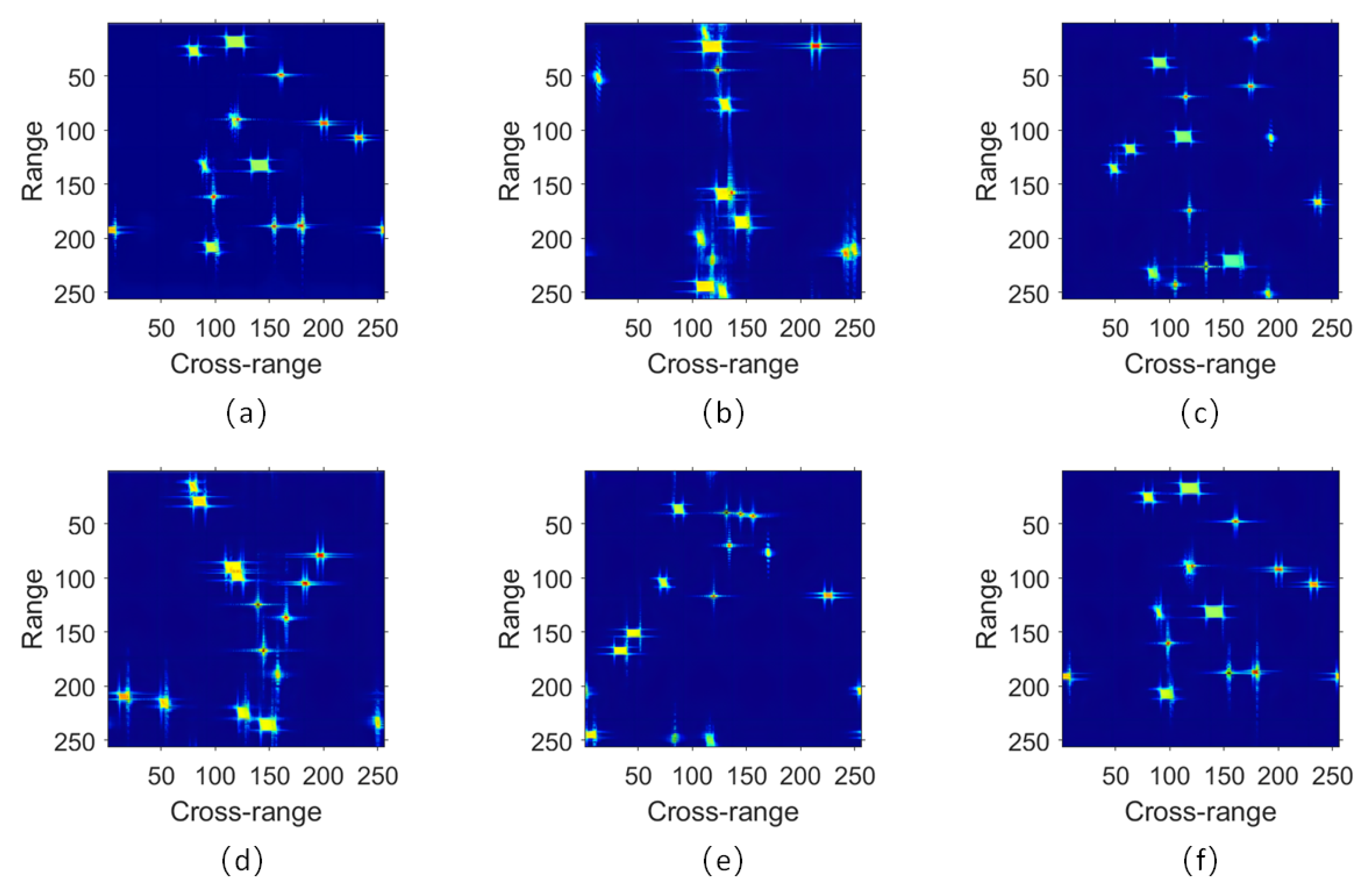
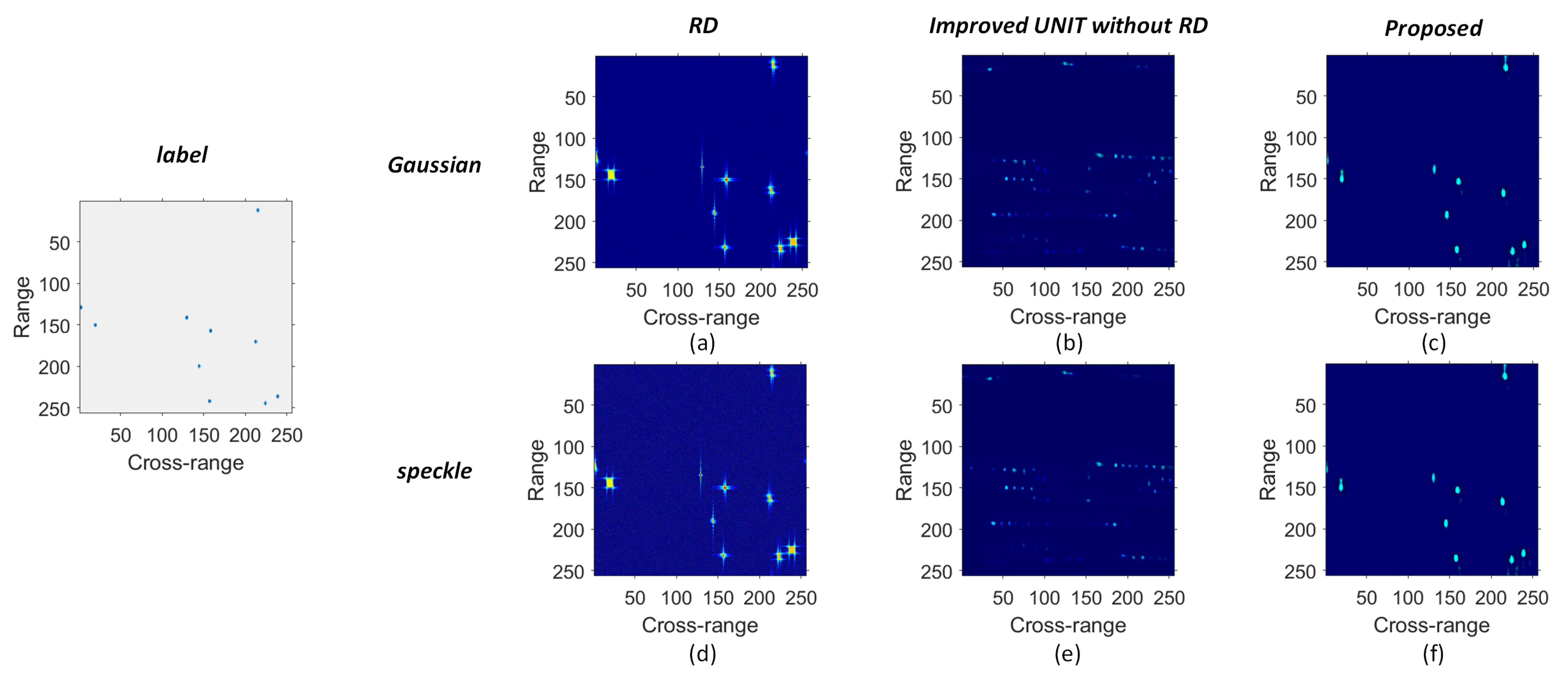
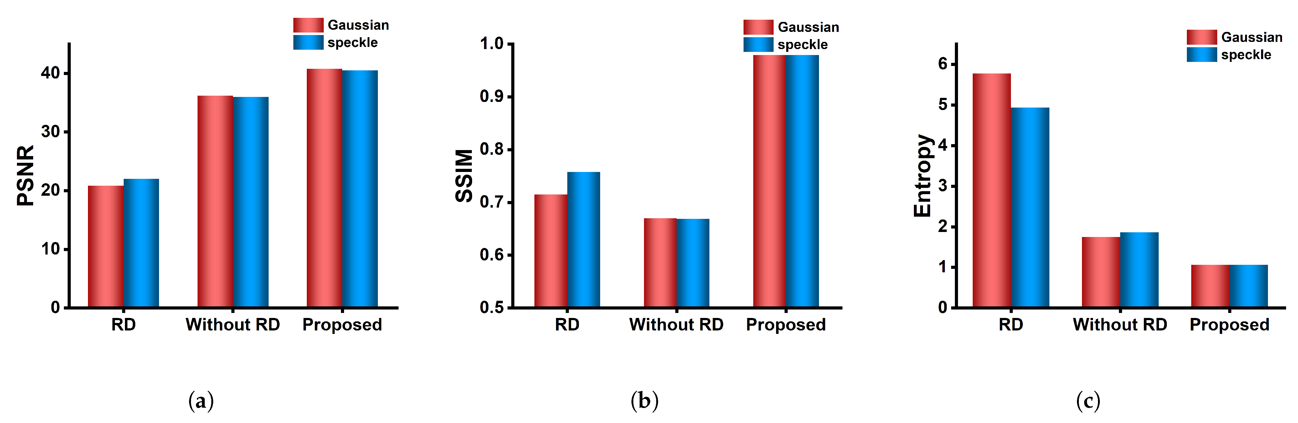
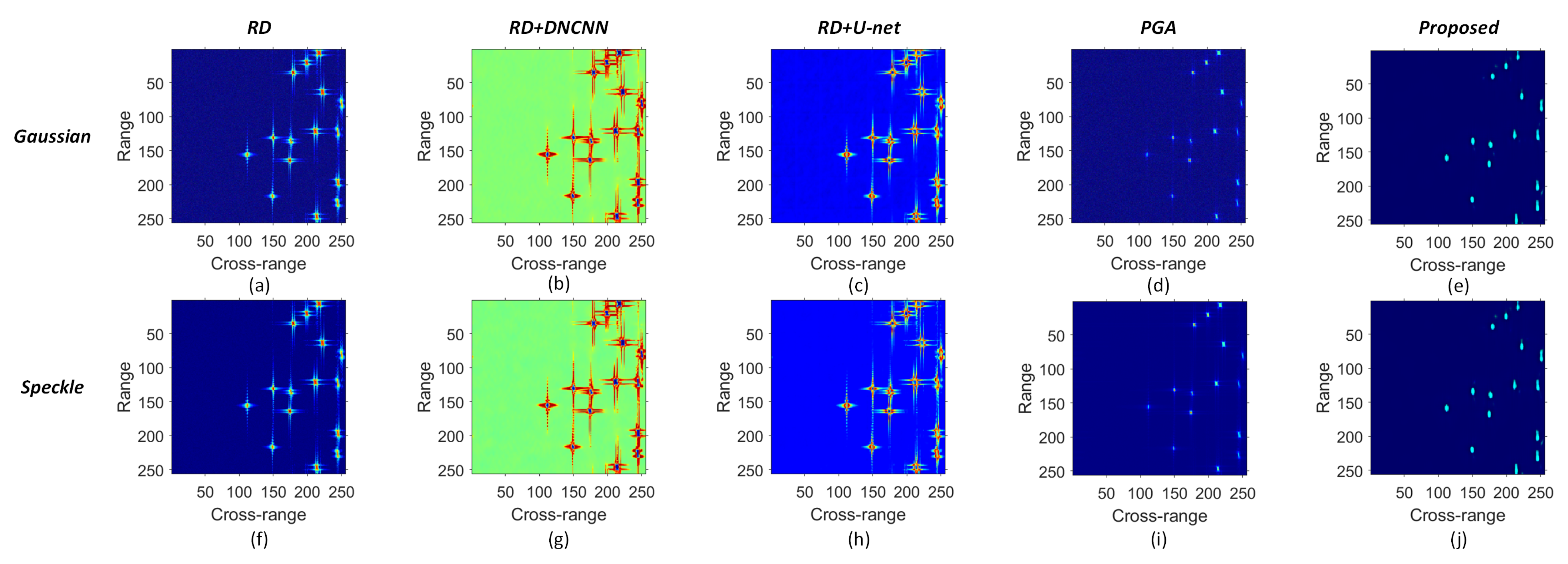
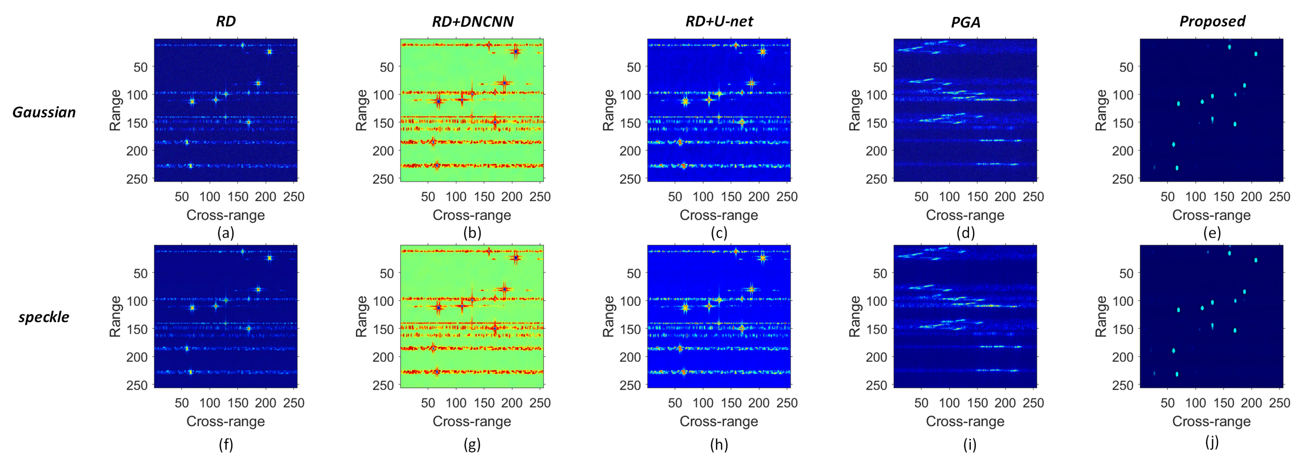
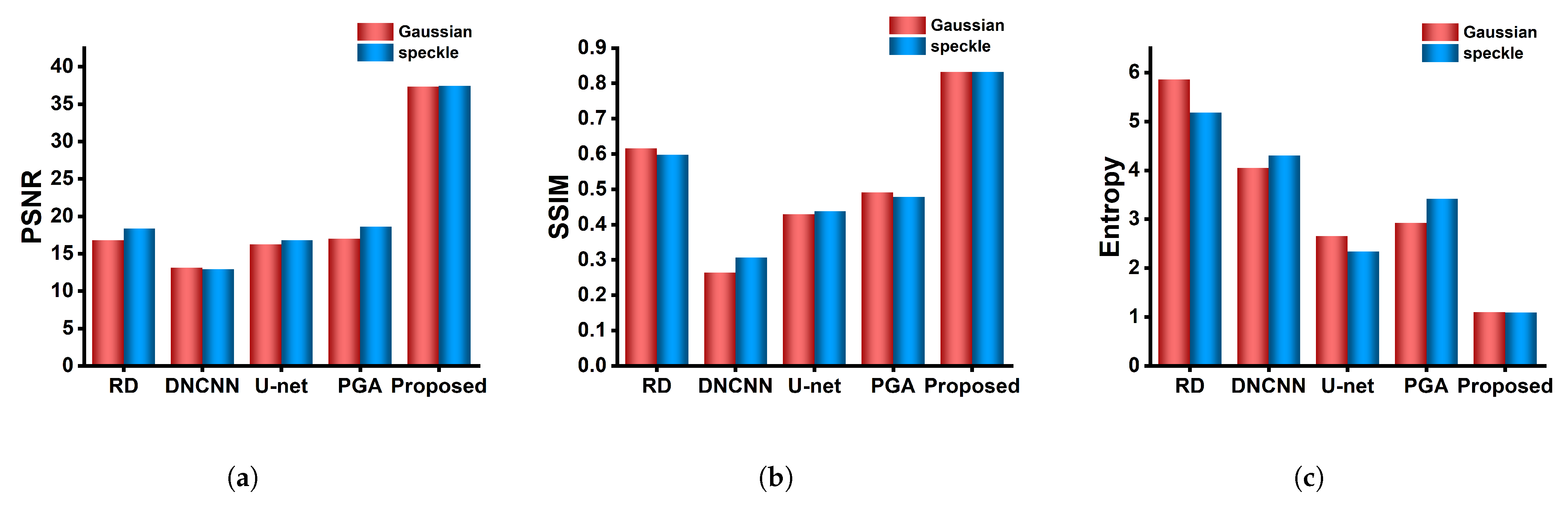
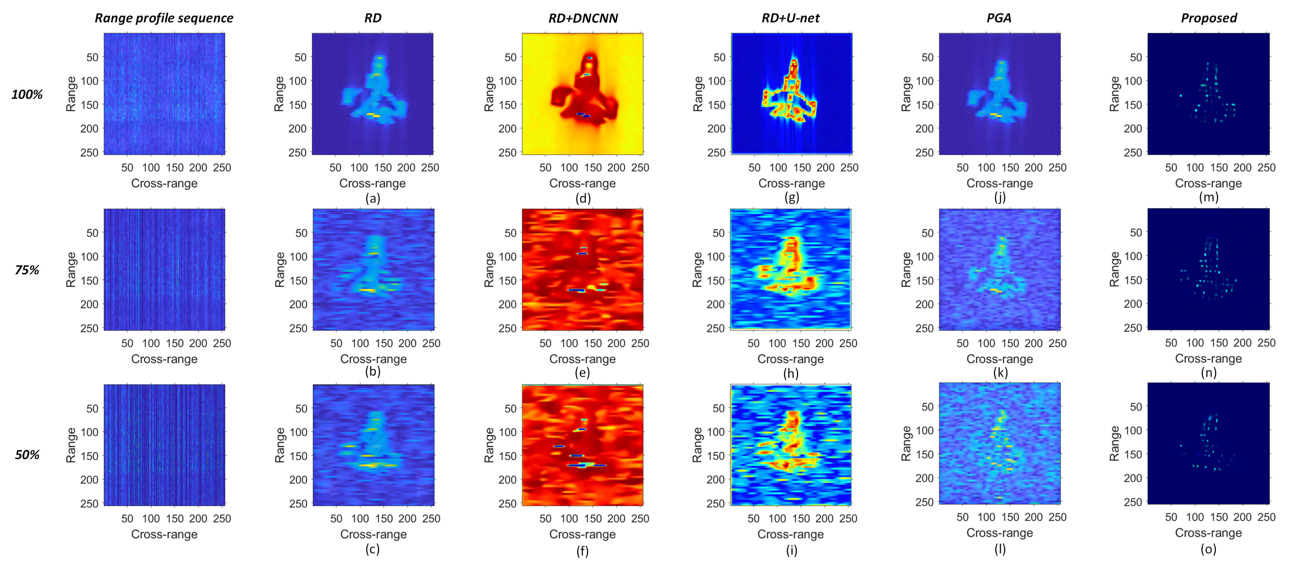
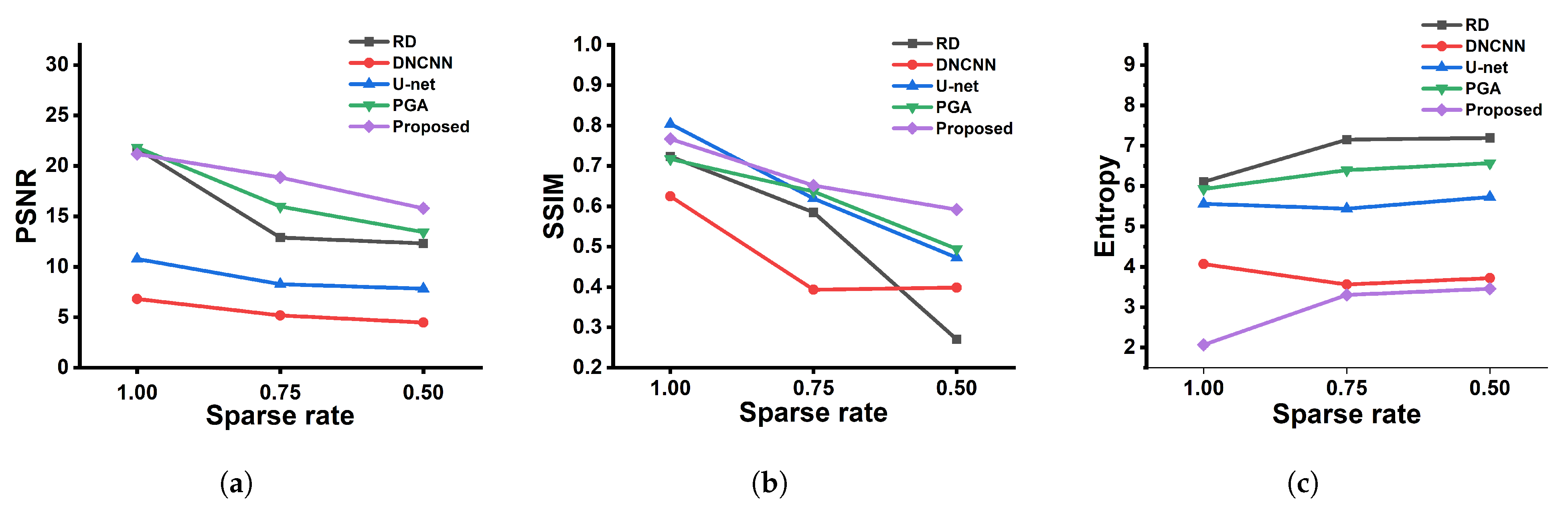
4.2. Experiment Results

Firstly, to verify the performance of our proposed model for ISAL imaging, we compare the RD algorithm, the improved UNIT without combining the RD algorithm, and our proposed model, respectively.
As shown in Figure 8, the image results of our proposed method are superior to those of the RD algorithm and the improved UNIT without RD. Figure 9 illustrates the numerical values of the different indexes. Our proposed method has higher PSNR and SSIM and lower entropy compared to the RD algorithm and improved UNIT without RD. These numerical results indicate that our proposed method achieves a less noisy background and better focus performance on the target.
Then, we test the point target in the turntable model when the target has only a rotational component. To study the robustness of our model in a real atmospheric environment, we introduce Gaussian or speckle noise to interfere with the background of the image.
Figure 10 shows the performance of the RD, RD+DNCNN, RD+U-net, PGA, and our proposed method for the turntable model. The inexact motion compensation of the radial motion of the target causes the RD images to be defocused and exhibit the MTRC phenomenon. The RD+DNCNN and RD+U-net methods have poor focusing performance in ISAL images. Both the PGA algorithm and our model both effectively restore the target shape, with our model exhibiting a better focused performance. For speckle noise, all the algorithms performed well. However, under Gaussian noise, the results of RD+U-net and RD+DNCNN do not completely eliminate the background noise in ISAL images. Our proposed model performed well under various noise conditions. Figure 11 illustrates that our proposed model achieved the highest PSNR and SSIM and the lowest entropy under various noise conditions.
Next, we change the input into a target that matches the real-world situation. In this case, the translation and rotation of the target occur simultaneously, and the target motion parameters are set randomly based on the cruising speed of the target in the airspace.
Figure 12 further shows the performance of various algorithms on ISAL images of scatter points in real-world situations. Unlike Figure 10, which only considers the turntable model, Figure 12 also introduces a translation component, further degrading the quality of the ISAL reconstructed image. As shown in Figure 12, the RD algorithm provides poor reconstruction results where the target points are no longer distinguishable in the azimuth direction in the upper part of the image. The rest of the generative models, as well as the PGA algorithm, did not perform well due to the lack of compensation for the phase errors caused by the non-radial motion of the target. Our proposed method, however, retains the main information of the target and eliminates background noise. Figure 13 illustrates that our proposed model achieves the highest PSNR and SSIM, and the lowest entropy for ISAL images of scatter points in real-world situations.
Finally, we applied our model to a real-world target: Mig-25, whose scattering point model is shown in Figure 14. We obtained the measured data of Mig-25 and sampled them at different sparsity rates. We set the sampling sparsity rates to 1, 0.75, and 0.5, respectively.
As shown in Figure 15, the quality of the ISAL image deteriorates significantly as the sparsity rate increases. The RD image becomes blurred, retaining only the outline of the target. The U-net result struggles to accurately identify the target type, and the PGA result is less effective in handling sparse data and high-frequency vibrations. Our proposed approach can recognize the main information of the target and effectively reduce background noise. However, it loses some target information under sparse conditions and reduces the brightness of the scattering points in the ISAL image. As shown in Figure 16, our proposed model achieved the highest PSNR and lowest entropy at high sparsity rates. For the SSIM, our model had the highest values when the sparsity rates were 0.75 and 0.5.

5. Conclusions

In this study, we designed a model combining an improved image translation network and the RD algorithm to estimate ISAL images, which has been experimentally shown to produce better ISAL images. Moreover, this method is sensitive to noise and maintains good image quality at different noise levels. The advantage of this method is that it provides good results even if the forward physical model does not accurately estimate the motion parameters of the target. The experimental results show that it meets the requirements of ISAL real-time image processing, both based on simulate data and real target imaging. However, under sparse aperture conditions, the ISAL signal still causes our proposed approach to lose some information about the target. In practical applications of ISAL, the target’s echo signal is often sparse, highlighting the limitations of our model in handling such scenarios. In the future, based on ISAL imaging theory, we will explore the application of complex-valued convolution in ISAL imaging or utilize transfer learning to improve the applicability of our proposed method. Additionally, reducing the computational complexity and training time of our model will be crucial to our future work.

Author Contributions

J.L. proposed the framework, design the experiment, and wrote the manuscript; B.W. and X.W. revised the manuscript. All authors have read and agreed to the published version of the manuscript.

Funding

This research was funded by the National Key Research and Development Program of China, grant number 2020YFA0714100; the National Natural Science Foundation of China, grant numbers 12171076 and 62135015; Science and Technology Department of Jilin Province, grant number 20210101146JC; and the Open Research Fund of KLAS, Northeast Normal University.

Data Availability Statement

The next steps are also based on this research, therefore it is not appropriate to share procedures of data at this time.

Conflicts of Interest

The authors declare no conflicts of interest.

References

  1. Hong, K.; Jin, K.; Song, A.; Xu, C.; Li, M. Low sampling rate digital dechirp for Inverse Synthetic Aperture Ladar imaging processing. Opt. Commun. 2023, 540, 129482. [Google Scholar] [CrossRef]
  2. Wang, N.; Wang, R.; Mo, D.; Li, G.; Zhang, K.; Wu, Y. Inverse synthetic aperture LADAR demonstration: System structure, imaging processing, and experiment result. Appl. Opt. 2018, 57, 230–236. [Google Scholar] [CrossRef] [PubMed]
  3. Liu, S.; Fu, H.; Wei, K.; Zhang, Y. Jointly compensated imaging algorithm of inverse synthetic aperture lidar based on Nelder-Mead simplex method. Acta Opt. Sin. 2018, 38, 0711002. [Google Scholar]
  4. Abdukirim, A.; Ren, Y.; Tao, Z.; Liu, S.; Li, Y.; Deng, H.; Rao, R. Effects of Atmospheric Coherent Time on Inverse Synthetic Aperture Ladar Imaging through Atmospheric Turbulence. Remote Sens. 2023, 15, 2883. [Google Scholar] [CrossRef]
  5. Berizzi, F.; Martorella, M.; Haywood, B.; Dalle Mese, E.; Bruscoli, S. A survey on ISAR autofocusing techniques. In Proceedings of the 2004 International Conference on Image Processing, Singapore, 24–27 October 2004; ICIP ’04. Volume 1, pp. 9–12. [Google Scholar] [CrossRef]
  6. Shakya, P.; Raj, A.B. Inverse Synthetic Aperture Radar Imaging Using Fourier Transform Technique. In Proceedings of the 2019 1st International Conference on Innovations in Information and Communication Technology (ICIICT), Chennai, India, 25–26 April 2019; pp. 1–4. [Google Scholar]
  7. Chen, V.C. Reconstruction of inverse synthetic aperture radar image using adaptive time-frequency wavelet transform. In Proceedings of the Wavelet Applications II, SPIE, Orlando, FL, USA, 17–21 April 1995; Volume 2491, pp. 373–386. [Google Scholar]
  8. Li, J.; Wu, R.; Chen, V. Robust autofocus algorithm for ISAR imaging of moving targets. IEEE Trans. Aerosp. Electron. Syst. 2001, 37, 1056–1069. [Google Scholar] [CrossRef]
  9. Xing, M.; Wu, R.; Bao, Z. High resolution ISAR imaging of high speed moving targets. IEE Proc.-Radar Sonar Navig. 2005, 152, 58–67. [Google Scholar] [CrossRef]
  10. Zhao, L.; Wang, L.; Bi, G.; Yang, L. An Autofocus Technique for High-Resolution Inverse Synthetic Aperture Radar Imagery. IEEE Trans. Geosci. Remote Sens. 2014, 52, 6392–6403. [Google Scholar] [CrossRef]
  11. Wang, X.; Guo, L.; Li, Y.; Han, L.; Xu, Q.; Jing, D.; Li, L.; Xing, M. Noise-Robust Vibration Phase Compensation for Satellite ISAL Imaging by Frequency Descent Minimum Entropy Optimization. IEEE Trans. Geosci. Remote Sens. 2022, 60, 1–17. [Google Scholar] [CrossRef]
  12. Xue, J.; Cao, Y.; Wu, Z.; Li, Y.; Zhang, G.; Yang, K.; Gao, R. Inverse synthetic aperture lidar imaging and compensation in slant atmospheric turbulence with phase gradient algorithm compensation. Opt. Laser Technol. 2022, 154, 108329. [Google Scholar] [CrossRef]
  13. Li, J.; Jin, K.; Xu, C.; Song, A.; Liu, D.; Cui, H.; Wang, S.; Wei, K. Adaptive motion error compensation method based on bat algorithm for maneuvering targets in inverse synthetic aperture LiDAR imaging. Opt. Eng. 2023, 62, 093103. [Google Scholar] [CrossRef]
  14. Lan, R.; Zou, H.; Pang, C.; Zhong, Y.; Liu, Z.; Luo, X. Image denoising via deep residual convolutional neural networks. Signal Image Video Process. 2021, 15, 1–8. [Google Scholar] [CrossRef]
  15. Shan, H.; Fu, X.; Lv, Z.; Xu, X.; Wang, X.; Zhang, Y. Synthetic aperture radar images denoising based on multi-scale attention cascade convolutional neural network. Meas. Sci. Technol. 2023, 34, 085403. [Google Scholar] [CrossRef]
  16. Lin, W.; Gao, X. Feature fusion for inverse synthetic aperture radar image classification via learning shared hidden space. Electron. Lett. 2021, 57, 986–988. [Google Scholar] [CrossRef]
  17. Huang, G.; Liu, Z.; Van Der Maaten, L.; Weinberger, K.Q. Densely connected convolutional networks. In Proceedings of the IEEE Conference on Computer Vision and Pattern Recognition, Honolulu, HI, USA, 21–26 July 2017; pp. 4700–4708. [Google Scholar]
  18. Krichen, M. Generative Adversarial Networks. In Proceedings of the 2023 14th International Conference on Computing Communication and Networking Technologies (ICCCNT), Delhi, India, 6–8 July 2023; pp. 1–7. [Google Scholar] [CrossRef]
  19. Yuan, Y.; Luo, Y.; Ni, J.; Zhang, Q. Inverse Synthetic Aperture Radar Imaging Using an Attention Generative Adversarial Network. Remote Sens. 2022, 14, 3509. [Google Scholar] [CrossRef]
  20. Yuan, H.; Li, H.; Zhang, Y.; Wang, Y.; Liu, Z.; Wei, C.; Yao, C. High-Resolution Refocusing for Defocused ISAR Images by Complex-Valued Pix2pixHD Network. IEEE Geosci. Remote Sens. Lett. 2022, 19, 1–5. [Google Scholar] [CrossRef]
  21. Xiao, C.; Gao, X.; Zhang, C. Deep Convolution Network with Sparse Prior for Sparse ISAR Image Enhancement. In Proceedings of the 2021 2nd Information Communication Technologies Conference (ICTC), Nanjing, China, 7–9 May 2021; pp. 54–59. [Google Scholar] [CrossRef]
  22. Liu, M.Y.; Breuel, T.; Kautz, J. Unsupervised Image-to-Image Translation Networks. In Proceedings of the Advances in Neural Information Processing Systems; Guyon, I., Luxburg, U.V., Bengio, S., Wallach, H., Fergus, R., Vishwanathan, S., Garnett, R., Eds.; Curran Associates, Inc.: Red Hook, NY, USA, 2017; Volume 30. [Google Scholar]
  23. Giusti, E.; Martorella, M. Range Doppler and image autofocusing for FMCW inverse synthetic aperture radar. IEEE Trans. Aerosp. Electron. Syst. 2011, 47, 2807–2823. [Google Scholar] [CrossRef]
  24. Othman, M.A.B.; Belz, J.; Farhang-Boroujeny, B. Performance Analysis of Matched Filter Bank for Detection of Linear Frequency Modulated Chirp Signals. IEEE Trans. Aerosp. Electron. Syst. 2017, 53, 41–54. [Google Scholar] [CrossRef]
  25. Chen, V.C.; Martorella, M. Inverse Synthetic Aperture Radar Imaging: Principles, Algorithms and Applications; The Institution of Engineering and Technology: London, UK, 2014. [Google Scholar]
  26. Zhang, S.S.; Zeng, T.; Long, T.; Yuan, H.P. Dim target detection based on keystone transform. In Proceedings of the IEEE International Radar Conference, Arlington, VA, USA, 9–12 May 2005; pp. 889–894. [Google Scholar] [CrossRef]
  27. Zhang, K.; Zuo, W.; Chen, Y.; Meng, D.; Zhang, L. Beyond a gaussian denoiser: Residual learning of deep cnn for image denoising. IEEE Trans. Image Process. 2017, 26, 3142–3155. [Google Scholar] [CrossRef] [PubMed]
  28. Ronneberger, O.; Fischer, P.; Brox, T. U-Net: Convolutional Networks for Biomedical Image Segmentation. arXiv 2015, arXiv:cs.CV/1505.04597. [Google Scholar]
  29. Fu, T.; Gao, M.; He, Y. An improved scatter selection method for phase gradient autofocus algorithm in SAR/ISAR autofocus. In Proceedings of the International Conference on Neural Networks and Signal Processing, Nanjing, China, 14–17 December 2003; Volume 2, pp. 1054–1057. [Google Scholar] [CrossRef]
Figure 1. ISAL imaging geometry model.
Remotesensing 16 02635 g001
Figure 2. Architecture of our proposed model.
Remotesensing 16 02635 g002
Figure 3. Sequence of ISAL range profiles generated by the range compensation: (a) echo signal after de-chirp frequency modulation; (b) aligned envelope.
Remotesensing 16 02635 g003
Figure 4. Single point target due to inaccurate compensation under ideal conditions: (a) RD image; (b) signal map.
Remotesensing 16 02635 g004
Figure 5. Network framework.
Remotesensing 16 02635 g005
Figure 6. (af) The training labels.
Remotesensing 16 02635 g006
Figure 7. (af) The ISAL images obtained by the RD algorithm.
Remotesensing 16 02635 g007
Figure 8. ISAL images with different constructions: (a,d) RD; (b,e) improved UNIT without RD; (c,f) proposed method.
Remotesensing 16 02635 g008
Figure 9. Numerical results for different methods: (a) PSNR; (b) SSIM; (c) Image entropy.
Remotesensing 16 02635 g009
Figure 10. ISAL images for the turntable model with different noises: (a,f) RD; (b,g) RD + DNCNN; (c,h) RD+U-net; (d,i) PGA; (e,j) proposed model.
Remotesensing 16 02635 g010
Figure 11. Numerical results for point targets in turntable model with different noise types: (a) PSNR; (b) SSIM; (c) Image entropy.
Remotesensing 16 02635 g011
Figure 12. ISAL images of scatter points of being in real-world situations with different noises obtained by different methods: (a,f) RD; (b,g) RD+DNCNN; (c,h) RD+U-net; (d,i) PGA; (e,j) proposed model.
Remotesensing 16 02635 g012
Figure 13. Numerical results for point targets in real-world situations with different noise types: (a) PSNR; (b) SSIM; (c) Image entropy.
Remotesensing 16 02635 g013
Figure 14. Airplane scatter points model for Mig-25.
Remotesensing 16 02635 g014
Figure 15. The image results on Mig-25 data under different sparsity rates: (ac) RD; (df) RD+DNCNN; (gi) RD+U-net; (jl) PGA; (mo) proposed model.
Remotesensing 16 02635 g015
Figure 16. Numerical results for Mig-25 data with different sparsity rates: (a) PSNR; (b) SSIM; (c) Image entropy.
Remotesensing 16 02635 g016
Table 1. Simulation parameters.
ParameterValue
Carrier frequency ( f c )193.5 THz
Bandwidth (B)10 GHz
Pulse width ( T a )25 μ s
Pulse repetition frequency (PRF)100 kHz
Laser wavelength ( λ )1550 nm
Table 2. Configurations of experimental environment.
ConfigurationParameter
CPUIntel(R) Core(TM) i9-13900K
GPUNVIDIA GeForce RTX 4090
Accelerated environmentCUDA11.8 CUDNN9.2.0
Disclaimer/Publisher’s Note: The statements, opinions and data contained in all publications are solely those of the individual author(s) and contributor(s) and not of MDPI and/or the editor(s). MDPI and/or the editor(s) disclaim responsibility for any injury to people or property resulting from any ideas, methods, instructions or products referred to in the content.

