Article

The Impact of Polar Vortex Strength on the Longitudinal Structure of the Noontime Mid-Latitude Ionosphere and Thermosphere

by
Loredana Perrone
1,* and
Andrey Mikhailov
2
1
Istituto Nazionale di Geofisica e Vulcanologia, Via di Vigna Murata 605, 00143 Rome, Italy
2
Pushkov Institute of Terrestrial Magnetism, Ionosphere and Radio Wave Propagation (IZMIRAN), Troitsk, 108840 Moscow, Russia
*
Author to whom correspondence should be addressed.
Remote Sens. 2024, 16(14), 2652; https://doi.org/10.3390/rs16142652 (registering DOI)
Submission received: 31 May 2024 / Revised: 10 July 2024 / Accepted: 15 July 2024 / Published: 20 July 2024

Abstract

:
Ground-based ionospheric, CHAMP/STAR, and GOCE satellite neutral density ρ observations under deep solar minimum conditions were used to find whether there is a dependence of longitudinal variations on polar vortex strength. Ionospheric stations at fixed-dipole geomagnetic Φ ≈ 38° and geographic φ ≈ 40°N latitudes located in ‘near-pole’ and ‘far-from-pole’ longitudinal sectors were used in the analysis. No significant longitudinal NmF2 (electron concentration in the F2-layer maximum) dependence on the polar vortex strength was revealed. Geomagnetic control was shown to be responsible for the observed longitudinal NmF2 variations. Satellite-observed longitudinal variations in neutral density did not show any visible reaction to the polar vortex strength. However, the impact of sudden stratospheric warming (SSW) on the upper atmosphere is strong enough to change the neutral density longitudinal distribution. The impact of SSW shows a global occurrence and ‘works’ within 3–5 days in geographic coordinates in the vicinity of the SSW peak. Atomic oxygen values retrieved under ‘strong’ and ‘weak’ polar vortex strengths confirm the results obtained on longitudinal variations in NmF2 and ρ. In conclusion, no visible effects related to ‘strong’ or ‘weak’ polar vortex strengths have been revealed in either NmF2 or satellite neutral density longitudinal variations. Alternatively, such effects may be very small and therefore cannot be confirmed experimentally.

1. Introduction

Historically, longitudinal variations in ionospheric and thermospheric parameters have been associated with high latitude heating and the displacement between the geomagnetic and geographic poles [1,2,3,4,5,6,7]. However, recently, due to increased interest in meteorological effects in the ionosphere and thermosphere, attempts have been made to reveal meteorological effects on longitudinal variations in ionospheric and thermospheric parameters. The most pronounced effects are related to major sudden stratospheric warmings (SSWs). It should be stressed that the majority of publications are devoted to the effects of SSWs in the mesosphere and low thermosphere, and the most pronounced thermo-ionospheric effects take place in the low-latitude and equatorial regions. We are interested in the meteorological effects observed in the thermosphere and ionosphere at middle latitudes. To avoid retelling the results of published papers, readers can refer to the comprehensive review in [8]. Model simulations are widely used in such analyses, although their correctness is always questionable, e.g., [9]; therefore, we do not discuss them here. Pertinent publications prior to 2022 were reviewed in our previous papers [10,11].
The next step in this direction is related to the analysis of the impact of polar vortex strength on the thermosphere and ionosphere. Based on WACCM-X model simulation results, the authors in [12] found a dependence of mesosphere and lower thermosphere (MLT) circulation on the polar vortex strength. Although their analysis was confined by MLT heights, they concluded that “…a strong stratospheric polar vortex can also have an appreciable impact on the middle and upper atmosphere”. The impact of the ‘weak’ polar vortex related to SSW on the ionosphere and thermosphere has been widely discussed in the literature, e.g., [8]. A new result obtained from the model simulations in [12] is that “ionosphere and thermosphere variability may also occur when the stratospheric polar vortex is strong”. Unfortunately, their simulation results were not compared to any direct ionospheric and thermospheric observations, so the validity of such conclusions is questionable. The authors themselves stress this, saying “it is therefore critical for the results of the present study to be confirmed observationally”.
Experimental support for this suggestion was provided in [13]. The authors compared one 3-day period in February 2008 with ‘weak’ polar vortex strength to another 3-day period in February 2021 with a ‘strong’ polar vortex. They found that “both weak and strong polar vortex conditions are associated with significant longitudinal variations in thermospheric composition and ionospheric plasma content at mid-latitudes”. A consideration of one case is not sufficient for such a conclusion. Moreover, geomagnetic activity was not low, with a daily Ap index up to 9–14 nT during the period in question (25–26 February 2021). Under deep solar minimum, such geomagnetic activity results in strong variations in ionospheric and thermospheric parameters at middle latitudes [10].
Therefore, additional analyses are required to find out whether polar vortex strength affects longitudinal variations in ionospheric and thermospheric parameters. An attempt at this has been undertaken in this paper using ground-based ionosonde and satellite neutral gas density observations during periods of deep solar minimum to avoid auroral heating effects as much as possible.
The aims of this paper can be formulated as follows:
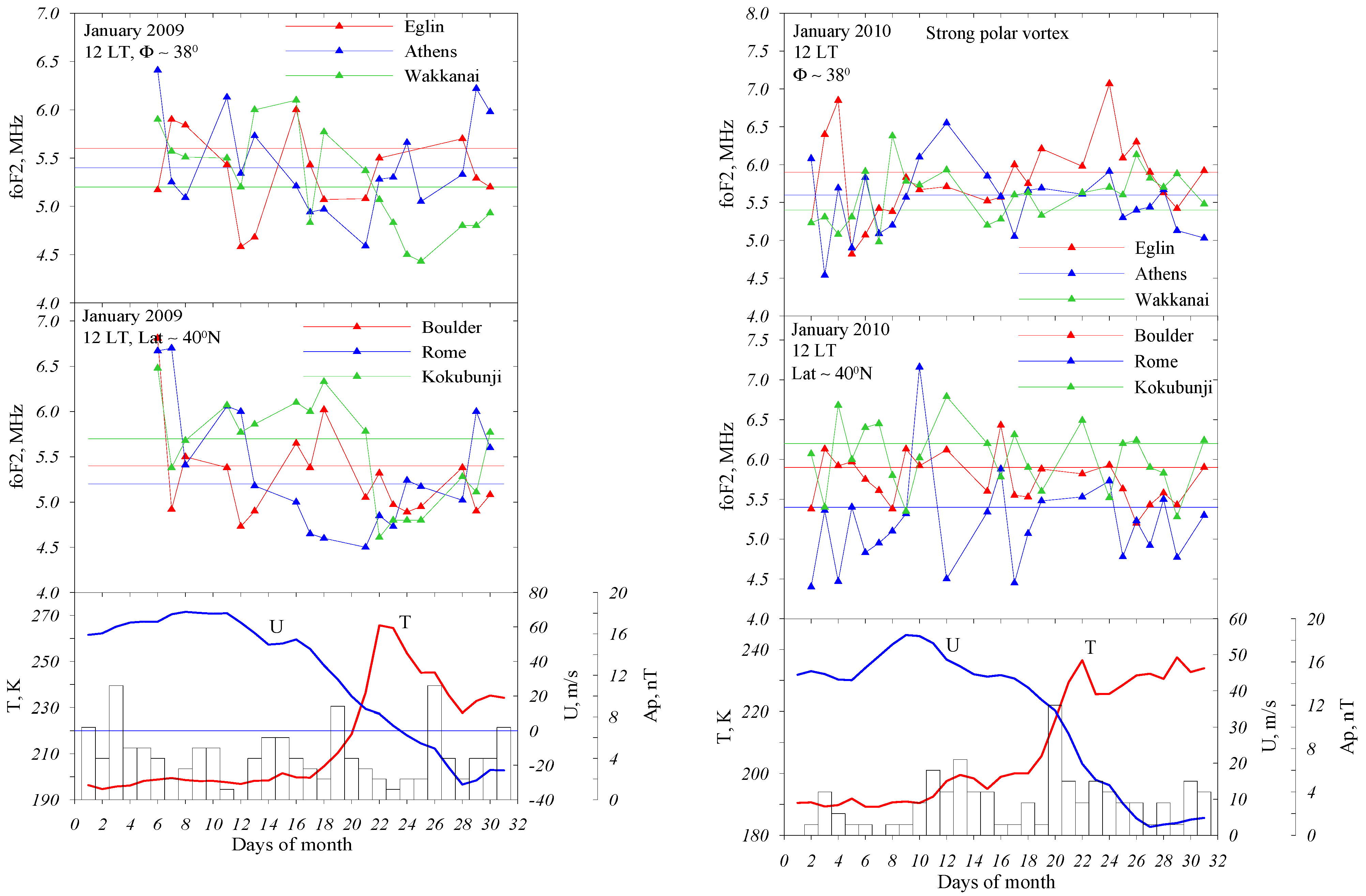
  • To consider longitudinal variations in noontime mid-latitude foF2 at ionosonde stations with close dipole magnetic and geographic latitudes located in ‘near-pole’ and ‘far-from-pole’ longitudinal sectors under ‘strong’ and ‘weak’ polar vortex strengths.
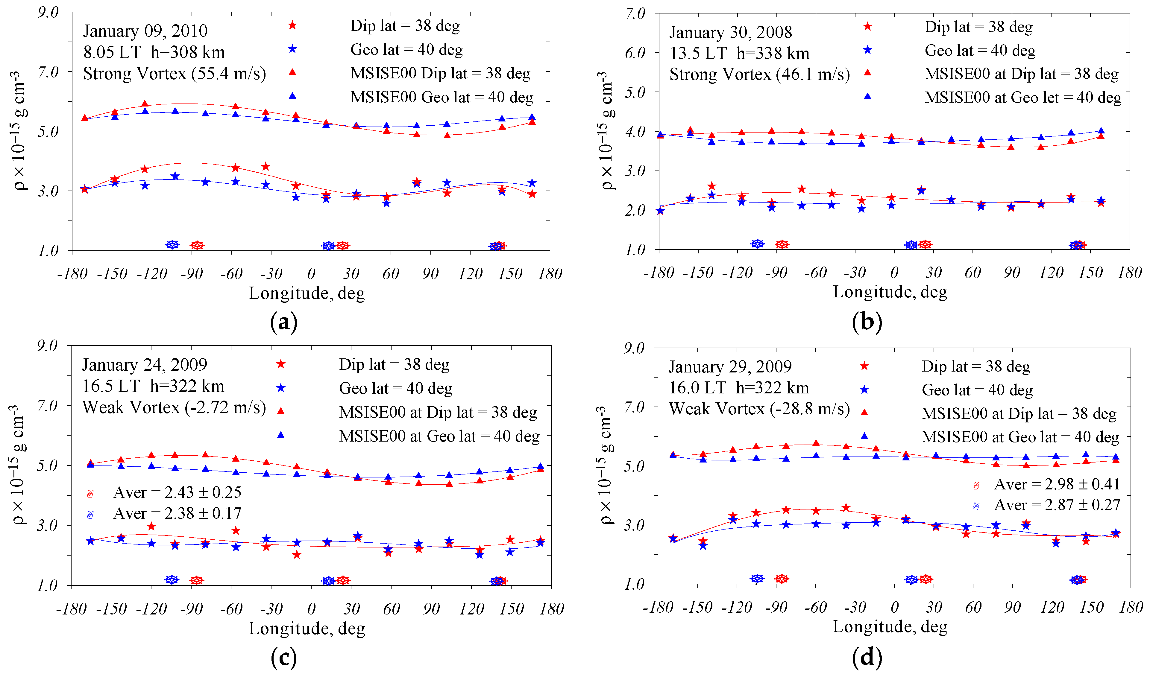
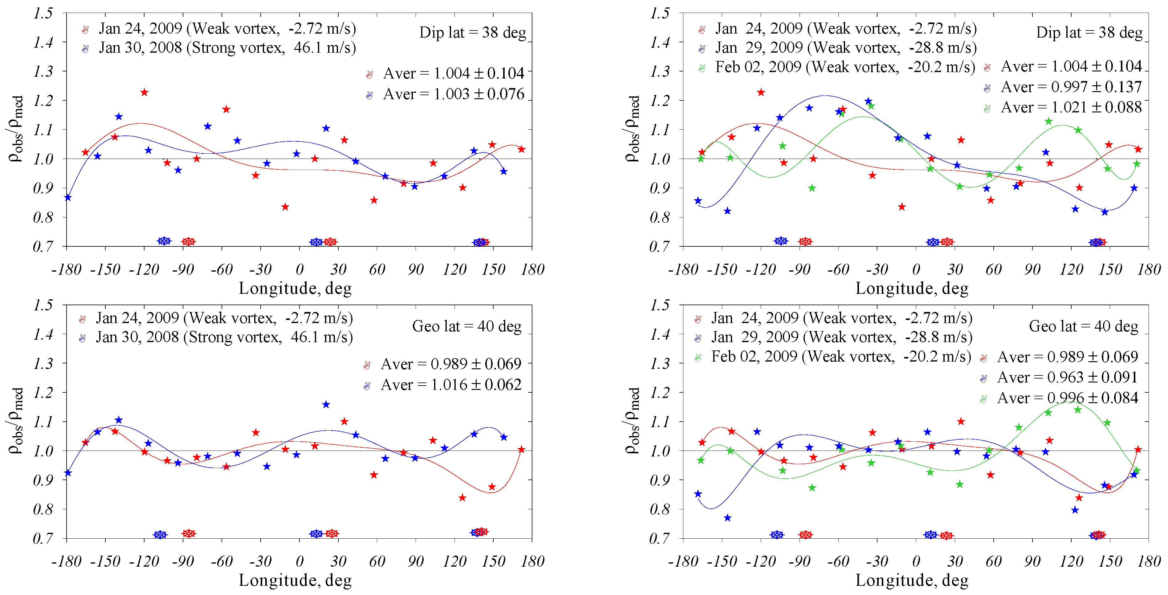
  • To analyze longitudinal variations in neutral density observed with CHAMP/STAR and GOCE satellites at fixed magnetic and geographic latitudes under ‘strong’ and ‘weak’ polar vortex strengths at middle latitudes during daytime hours.
  • To retrieve thermospheric parameters using ionosonde and satellite neutral density observations for periods of ‘strong’ and ‘weak’ polar vortex strength to conclude whether polar vortex strength impacts the thermospheric state.
  • To discuss the possible mechanisms of the impact of polar vortex on the thermosphere and ionospheric F2-region.

2. Observations and the Method of Analysis

For our analysis, we selected three mid-latitude ionospheric stations with close dipole magnetic latitudes Φ, Wakkanai (45.4°N, 141.7°E, Φ = 36.9°), Athens (38.0°N, 23.6°E, Φ = 36.3°), and Eglin (30.5°N, 273.5°E, Φ = 40.0°), and three stations with close geographic latitudes, Kokubunji (35.7°N, 139.5°E, Φ = 26.9°), Rome (41.8°N, 12.5°E, Φ = 41.7°), and Boulder (40.0°N, 254.7.5°E, Φ = 47.9°). Dipole magnetic latitudes are given for the 2010 epoch (wdc.kugi.kyoto-u.ac.jp/igrf/gggm/, accessed on 1 July 2024). The terms ‘near-pole’ and ‘far-from-pole’ stations were introduced by Rishbeth and Müller-Wodarg [14] to specify the position of a station with respect to the magnetic pole. Therefore, America is a ‘near-pole’ longitudinal sector, while Eurasia is ‘far-from-pole’one. According to [14], the stations located in ‘near-pole’ and ‘far-from-pole’ longitudinal sectors with respect to the magnetic pole are subjected to different auroral heating impacts. The longitudinal difference between the stations is around 130°, and this is sufficient to make a conclusion on the longitudinal global-scale variations in noontime foF2. To minimize auroral effects, deep solar minimum conditions in 2009–2010 and 2020–2021 with daily Ap ≤ 4 nT for current and Ap ≤ 6 nT for previous days were analyzed. One may hope that under such conditions the auroral impact will be minimal and meteorological effects related to the polar vortex strength will be visible. Observed hourly foF2 values were taken from SPIDR, GIRO, and NICT sites. Second-order polynomial approximation was applied to five (10–14)LT foF2 values to read from this approximation noontime foF2.
Longitudinally averaged zonal stratospheric wind U at 10 hPa (~32 km) and 60°N is an indicator of the polar vortex strength (https://acdext.gsfc.nasa.gov/Data_services/met/ann_data_help.html, access date 15 November 2023). According to MERRA-2, the breakdown of the polar vortex occurs when stratospheric zonal wind U drops below about 15 m/s. To avoid overlapping of the two arrays, days with U ≤ 3 m/s were considered as days with ‘weak’ polar vortex strength, while days with U ≥ 35 m/s were referred to as ‘strong’ polar vortex conditions.
Winter through spring is the period with the largest variations in stratospheric zonal wind, and the breakdown of the polar vortex results in SSWs. Therefore, January–February 2009 and 2010, March 2010, and January 2020 and 2021 were selected for our analysis. Although ionizing solar EUV flux demonstrated small variations during the periods in question under solar minimum [15,16], the analyzed noontime NmF2 = 1.24 × 10⁴(foF2)2 was reduced on the ionizing EUV flux using the EUV model [16] to ensure that the impact of EUV was excluded. However, the analysis has shown that the effect of this reduction is very small, as was expected under solar minimum conditions.

3. Results

The longitudinal variations under strong and weak vortex strength were analyzed by comparing LogNmF2 between pairs of stations with close dipole magnetic and geographic latitudes. A Student’s t-test was used to estimate the significance of longitudinal differences.
Table 1 shows that there is no significant longitudinal difference in NmF2 between ‘strong’ and ‘weak’ polar vortex strengths for stations with close dipole magnetic latitudes. This means that the geomagnetic control of longitudinal variations in NmF2 dominates over the polar vortex impact, if the latter exists. Such impact from below does exist during SSW (‘weak’ polar vortex); in this case, we should accept that the magnitude of this impact is less than that of the geomagnetic control, or it works in the same direction to decrease longitudinal differences in NmF2. The latter seems to be confirmed by the results obtained for Eglin/Athens (Table 1). Adding SSW effects decreases the t-parameter; i.e., the longitudinal difference in NmF2 decreases.
Stations with close geographic latitudes demonstrate different results. Under the ‘strong’ polar vortex strength, when no impact from below is expected (no SSW events), we observe statistically significant NmF2 longitudinal variations due to the different geomagnetic latitudes of the stations in question, i.e., we see the results of NmF2 geomagnetic control. However, these longitudinal differences are strongly decreased under the ‘weak’ polar vortex strength (see t-parameter in Table 1). This means that the impact of SSW overlaps with that of the geomagnetic field, strongly dampening it and resulting in insignificant longitudinal differences between stations (compare the t-parameters in Table 1). Thus, we should accept that the impact of SSW is comparable to or stronger than the geomagnetic impact in decreasing the scatter in NmF2 related to the different geomagnetic latitudes of the stations. It should be recalled that the geomagnetic control of NmF2 is used in the IRI model ([17] and references therein) to decrease longitudinal variations in global mapping procedures for is foF2.
It should be stressed that noontime mid-latitude NmF2 depends not only on thermospheric neutral composition, but also on vertical plasma drift. This is represented by the equation W = VnxsinIcosIcosD, where Vnx is the meridional component of thermospheric wind, I is the magnetic inclination, and D is the magnetic declination. The contribution of the zonal Vny component of thermospheric wind is small around noontime hours at middle latitudes [18,19]. Therefore, stations with close geographic latitudes will be subjected to different W due to different magnetic inclination under the same Vnx. This may be an additional reason for the significant longitudinal difference in NmF2 at the stations with close geographic latitudes (Table 1).
The statistical results given in Table 1 are illustrated by Figure 1 for a major SSW with its peak on 23 January 2009. This is an excellent example of SSW that is not contaminated with geomagnetic activity effects under deep solar minimum. The period includes days with ‘strong’ and ‘weak’ polar vortex strengths. The earlier considered stations with close geomagnetic and geographic latitudes were used for this illustration. It is seen that stations with Φ~38° manifest just a scatter of foF2 values, in accordance with Table 1.
Stations with close geographic latitudes (~40°N) demonstrate interesting results. In accordance with the results in Table 1, a well-pronounced longitudinal difference between stations is seen during 12–22 January, when polar vortex was positive and mainly ‘strong’. However, after 23 January, the difference in foF2 between stations strongly decreased, clearly indicating the impact of SSW. Such foF2 variations tell us that the impact of SSW has a global occurrence and ‘works’ in geographic coordinates. According to the results in Table 1, there is no longitudinal difference in foF2 in this case. It should be noted that the foF2 scatter is decreased for only ~5 days after the SSW peak. This issue will be discussed later.
Figure 1 (right panels) gives an illustration of the impact of the ‘strong’ polar vortex on foF2 in January 2010. That was also a period practically free of magnetic disturbances under deep solar minimum. The dates of 1–20 January with U ≥ 35 m/s were selected for our analysis. A Student’s t-test was used to estimate the significance of differences in foF2 between stations. The difference between the Eglin and Athens stations is insignificant (t = 0.84), as is that between Eglin and Wakkanai (t = 1.23). Therefore, the selected illustrative period has shown that, in agreement with the results in Table 1, stations with close magnetic latitudes do not show any significant longitudinal differences in foF2 under the ‘strong’ polar vortex strength. On the other hand, stations with close geographic latitudes demonstrate significant longitudinal differences in foF2 during the period 1–20 January 2010. The difference between the Boulder and Rome stations is significant at the 99.7% (t = 3.30) confidence level, and that between Boulder and Kokubunji is significant at the 95.0% level (t = 2.05). The degrees of freedom, m, was equal to 30 for all cases in question.
The undertaken analysis has shown that a ‘strong’ polar vortex does not affect the noontime mid-latitude foF2, producing no longitudinal foF2 variations for the stations with close magnetic latitudes. Stations with close geographic latitudes manifest significant differences in longitudinal foF2 variations, but this effect is related to the different magnetic latitudes of these stations and has nothing to do with the polar vortex strength.
The ‘weak’ polar vortex related to SSW shows an obvious impact on foF2, and this has been discussed in many publications [11,20,21,22,23]. According to our concept [10,11], the effect is due to the intensification of eddy diffusion, leading to a decrease in the atomic oxygen abundance in the thermosphere. The results of the present analysis (and also those of [11]) tell us that the impact of SSW has global occurrence at middle latitudes and that it ‘works’ in geographic coordinates.
Satellite neutral gas density ρ observations from CHAMP/STAR (http://[email protected]/champ, access date 1 January 2024) and GOCE (http://thermosphere.tudelft.nl/, access date 1 January 2024) may be used to check the above obtained results on longitudinal variations for the periods of ‘strong’ and ‘weak’ polar vortex strength. It should be recalled that neutral density at satellite heights mainly presents atomic oxygen abundance, so such ρ observations can inform us about longitudinal variations in [O]. In turn, according to [24],
NmF2~IEUV × [O]4/3
where IEUV is the intensity of ionizing EUV radiation, and the atomic oxygen concentration [O] is taken at a fixed height. Therefore, with earlier mentioned reservations for the vertical plasma drift W, atomic oxygen is the controlling parameter for NmF2 variations; therefore, the observed ρ and retrieved [O] will be discussed together with longitudinal variations in NmF2. Two pairs of days with ‘strong’ and ‘weak’ polar vortex strengths are given in Figure 2. The days with a ‘weak’ polar vortex belong to the same SSW event in January–February 2009 (Figure 2c,d), with 24 January being next to the SSW peak, while 2 February is eight days later. Both days with ‘weak’ polar vortexes were under very low geomagnetic activity (all ap-3 h ≤ 4 nT for 24 January and ≤2 nT for 2 February) and the same low (F10.7 ≈ 69) level of solar activity. This is necessary to be sure that the observed difference between the two dates can be attributed to the meteorological impact.
Figure 2 shows that MSISE00 [25] demonstrates small longitudinal variations at geographic latitude 40°N, but this dependence can be clearly observed at dipole latitude 38°, with a larger ρ in the ‘near-pole’ American sector compared to the ‘far-from-pole’ Eurasian one. A similar tendency is seen for the satellite-observed ρ under a ‘strong’ vortex strength (Figure 2a,b). In general, neutral density increases towards the equator in winter, and points with Φ = 38° located at lower geographic latitudes in the ‘near-pole’ sector manifest larger ρ; the opposite takes place in the ‘far-from-pole’ sector. Therefore, dates with a ‘strong’ polar vortex strength manifest normal longitudinal variations in neutral density implemented in the empirical MSISE00 model.
The situation with the ‘weak’ polar vortex is different. Observed longitudinal variations in ρ are not pronounced, and the curves for Φ = 38° and φ = 40°N are close to each other (see average values in Figure 2c,d). This is especially true for 24 January, the peak of the SSW. This may indicate that the impact of SSW is stronger than the geomagnetic impact, and that this impact ‘works’ in geographic coordinates, confirming the earlier obtained result. Eight days later (on 2 February), the longitudinal variations in ρ look more similar to those in the MSISE00 model (Figure 2d).
In accordance with the results in [11], confirmed by direct WIND Imaging Interferometer on UARS [26] observations, the SSW impact on atomic oxygen concentration takes place only for only 3–5 days in the vicinity of the SSW peak; therefore, by 8 days after the SSW peak, the thermosphere should restore to its normal state. We do not discuss the absolute shift between the model and observed ρ values (Figure 2), which is mainly due to the overestimated Tex in MSISE00, according to [27].
The neutral density variations from Figure 2 were further analyzed to check whether different polar vortex strengths could be seen in the observed longitudinal variations in ρ. The ratios of the observed to median neutral density were calculated for the dates in Figure 2, and these δ = ρobsmed are given in Figure 3. The left panels in Figure 3 give a comparison of 30 January 2008 (a strong polar vortex strength, 46.1 m/s) and 24 January 2009 (a weak vortex strength, −2.72 m/s) for ρ observed at Φ = 38° and φ = 40°N. Both approximation curves manifest longitudinal variations within ±10%, and this is within the inaccuracy range ± (10–15%) of CHAMP/STAR neutral gas density observations [28]. The average δ values given in the plots also do not show any statistically significant difference for these two dates. It should be recalled that geomagnetic activity was very low for both dates. Therefore, a comparison of satellite-observed longitudinal variations in ρ under ‘strong’ and ‘weak’ polar vortex strengths does not show any significant difference. Alternatively, it is possible to say that the accuracy of existing thermospheric parameter observation methods is not sufficient to see this difference.
More pronounced longitudinal variations in δ are observed during the January–February 2009 SSW under ‘weak’ polar vortex strengths (Figure 3, right panels). 2 February demonstrates wave-type longitudinal variations in δ that are presumably related to wave processes in the stratosphere, as solar and geomagnetic activity were at the lowest level on that day. 29 January manifests ± 20% variations in δ, with the largest ρ in the American sector and the lowest ρ in the Japanese one. This was four days after the SSW peak and one may think that, in accordance with the results in [11,26], the effects of SSW should not be seen in the thermosphere. Therefore, the observed effects in ρ should be attributed to geomagnetic activity variations. Although 29 January was magnetically quiet with daily Ap = 4 nT, ap-3 h indices were up to 7–9 nT at (06–09)UT, with splashes of AE-index up to 212 nT. This increase in auroral activity resulted in larger ρ values, higher Tex, and larger retrieved [O] and [N2] in the American sector (Table 2, see later) compared to 24 January 2009. Therefore, the observed well-pronounced longitudinal variations in ρ on 29 January are not related to the polar vortex strength of −28.8 m/s, but reflect a reaction to increased auroral activity, which was not strong and was only short-term.
The last step in our analysis was to retrieve thermospheric parameters at Eglin, Athens, Boulder and Rome for 30 January 2008 (‘strong’ polar vortex); 29 January 2009 (‘weak’ polar vortex); and 24 January 2009 (‘weak’ polar vortex next to the SSW peak). Our method [29] to retrieve thermospheric parameters requires bottom-side Ne(h) profile and satellite neutral gas density observations, so only stations with DPS-4 [30] installed could be used. This method has been used in many of our previous papers, e.g., [31,32,33], so its description is not repeated here. The results are given in Table 2.
Stations with close geographic latitudes (Boulder/Rome) show large longitudinal differences of 48% in ρ, 19.5% in [O]300, and 74% in [N2]300 under the ‘strong’ polar vortex. This agrees with the results for longitudinal variations in NmF2 (Table 1) under the same conditions. Stations with close geomagnetic latitudes (Eglin/Athens) show much smaller longitudinal differences of 3% in ρ, 10% in [O]300, and 8% in [N2]300 under the ‘strong’ polar vortex. An insignificant longitudinal difference in NmF2 was obtained earlier for these stations under the same condition (Table 1).
Depending on the closeness of the date to the SSW maximum, the longitudinal difference between stations is different under the ‘weak’ vortex strength. Stations with close geographic latitudes (Boulder/Rome) show a very small difference, i.e., 7% in ρ, 3% in [O]300, and 8% in [N2]300, compared with the same stations under the ‘strong’ polar vortex (see earlier). This result is a direct confirmation of the earlier obtained conclusion that the impact of SSW is stronger than or comparable to the geomagnetic impact, and that it ‘works’ in geographic coordinates. Unfortunately, SAO files with Ne(h) profiles were absent at Eglin for 24 January, and neutral composition could not be retrieved for this station. 2 February was also a day with a ‘weak’ polar vortex strength, but it is far away from the date of the SSW maximum (24 January), and in accordance with our concept, it should not be used to attempt to demonstrate the impact of SSW. Indeed, the difference between the Boulder and Rome stations is 17% for [O]300 and 44% for [N2]300 (Table 2); this is close to the differences obtained for this pair of stations under the ‘strong’ polar vortex (see earlier).

4. Discussion

The available observations and data analysis methods are sufficient to answer the question of whether polar vortex strength can produce visible and statistically significant effects in the upper atmosphere and ionosphere. According to the theory of the F2-layer, daytime NmF2 at middle latitudes directly reflects the state of the surrounding thermosphere, particularly the atomic oxygen concentration. Therefore, ground-based ionosonde NmF2 observations can be successfully used to analyze longitudinal variations in the thermosphere, unlike the widely used TEC data, which depend not only on NmF2, but also on plasma-scale height and the plasmaspheric contribution; these latter two factors are routinely unknown. A poor relationship between TEC and column O/N2 GUVI observations was demonstrated in Figure 8 of [13].
The mid-latitude daytime ionospheric F2-layer is strongly controlled by geomagnetic activity via thermospheric parameters; this geomagnetic impact is dependent on the solar activity level. For instance, days with daily Ap = 10–12 nT may be considered magnetically quiet under solar maximum, while magnetic disturbances with daily Ap ≤ 7 nT can produce strong NmF2 perturbations under solar minimum [10]. For this reason, deep solar minimum days with Ap ≤ 4/6 nT were selected for our analysis to avoid auroral heating effects as much as possible.
Our analysis has not revealed any visible or statistically significant effects of polar vortex strength on longitudinal variations in either NmF2 or thermospheric parameters. This may tell us that such effects are either absent or very small and cannot be reliably detected. According to WACCM-X simulations [33], “weak stratosphere polar vortex times are associated with a 3–4% reduction in ΣO/N2, while strong stratosphere polar vortex time periods are associated with a 1–2% increase in ΣO/N2”. This means that such small effects cannot be confirmed experimentally using present-day thermospheric observation methods. Therefore, one case study [13] cannot serve as a confirmation of the presence of polar vortex strength effects, and more statistics are required. Our analysis has demonstrated a strong impact of auroral activity on longitudinal variations in ρ, even under the magnetically quiet conditions of 29 January 2009, with daily Ap = 4 nT. Meanwhile, the results in [13] were obtained under an Ap index up to 9–14 nT during the period in question (25–26 February 2021).
While our analysis has shown that stations with close geographic latitudes manifest a statistically significant NmF2 longitudinal dependence under ‘strong’ polar vortex (Table 1), this just indicates the absence of any impact from outside and that longitudinal variations in NmF2 are just related to the different geomagnetic latitudes of the stations, i.e., we see the results of geomagnetic control. In this case, under a ‘strong’ vortex, stations with close geomagnetic latitudes did not manifest any significant longitudinal variations in NmF2 (Table 1).
The situation under a ‘weak’ polar vortex is more interesting. ‘Weak’ vortexes are associated with SSW, which produces visible effects in the thermosphere and ionosphere. This has been demonstrated in many publications. However, not all cases of ‘weak’ polar vortexes result in visible effects, only those that occur in the vicinity (3–5 days) of the SSW maximum. Days that are far away in time from the SSW peak, even with large negative zonal winds, do not manifest visible effects. The results of the present analysis (see also [10]), as well as the WIND Imaging Interferometer on UARS observations [26], seem to confirm this conclusion.
The impact of SSW shows a global occurrence, and is stronger than or comparable to the geomagnetic impact; therefore, longitudinal differences in NmF2 are strongly dampened under the ‘weak’ polar vortex (Figure 1). Although the Student’s t-parameter is not small, especially for stations with close geographic latitudes (Boulder, Rome, and Kokubunji), it is not sufficient, even at a 95% significance level. We put together all days with U ≤ 3 m/s as ‘weak’ polar vortex cases without any discrimination with respect to the SSW peak. For this reason, days close to and far away from the SSW peak were included in general statistics. One may think if NmF2 data were discriminated with respect to the SSW peak, the results would be different, and cases within 3–5 days of the SSW peak would demonstrate an absence of any longitudinal difference. The observed neutral densities (Figure 2, 24 January) and retrieved [O] (Table 2, 24 January) seem to confirm this suggestion.

5. Conclusions

The obtained results can be summarized as follows:
  • Stations located at close dipole geomagnetic latitudes ≈ 38° show statistically insignificant longitudinal variations in NmF2 under both ‘strong’ and ‘weak’ vortex strengths. The absence of significant longitudinal variations in NmF2 is the manifestation of the well-known geomagnetic control in the F2-region. The impact from below during SSW (‘weak’ polar vortex) working in the same direction as the geomagnetic control further decreases the longitudinal difference in NmF2.
  • Stations with close geographic latitudes ≈ 40°N show well-pronounced and statistically significant longitudinal variation under the ‘strong’ polar vortex when no SSW effects are expected. However, this effect is related to different magnetic latitudes of the stations and has nothing to do with the polar vortex strength. The impact of SSW under the ‘weak’ polar vortex overlaps with that of the geomagnetic field and strongly dampens it, resulting in insignificant longitudinal differences between stations.
  • The satellite-observed longitudinal variations in neutral density do not show any visible reaction to the polar vortex strength, but mainly reflect dependence on the standard geophysical parameters used in empirical thermospheric models like MSISE00. However, the dependence on polar vortex can be seen under the SSW (‘weak’ polar vortex) event, where there are no pronounced longitudinal variations in the satellite-observed ρ values at either Φ = 38° or φ = 40°N. This coincidence of neutral density at magnetic and geographic latitudes tells us that the impact of SSW on the upper atmosphere is strong enough to change the normal pattern of ρ’s longitudinal distribution. The impact of SSW shows a global occurrence and ‘works’ within 3–5 days in geographic coordinates in the vicinity of the SSW peak.
  • The thermospheric parameters retrieved under ‘strong’ and ‘weak’ polar vortex strengths at stations separated in longitude confirm the results obtained on the longitudinal variations in NmF2 and neutral density.
  • The final result of our analysis is as follows: no visible effects related to ‘strong’ or ‘weak’ polar vortex strengths have been revealed for longitudinal variations in either NmF2 or satellite-observed neutral density confirmed by the retrieved thermospheric parameters. Alternatively, such effects may be very small, and thus cannot be confirmed experimentally. However, the impact on longitudinal variations in thermospheric (neutral density and atomic oxygen) and ionospheric NmF2 is clearly shown during SSW (‘weak’ polar vortex) events. However, this SSW impact has nothing to do with the polar vortex strength. It is related, as shown earlier, to a decrease in the atomic oxygen abundance in the thermosphere during SSW events.

Author Contributions

Conceptualization, A.M. and L.P.; methodology, A.M. and L.P.; software, L.P. and A.M.; data preparation, L.P. and A.M.; writing, A.M. and L.P. All authors have read and agreed to the published version of the manuscript.

Funding

This research was carried out within the INGV Pianeta Dinamico Project (CUP D53J19000170001), Space weather effects on the South Atlantic anomaly Region (SESAR)–2021, funded by MUR (law 145/2018).

Data Availability Statement

The data presented in this study are available on request from the corresponding author.

Acknowledgments

The authors thank the GFZ German Research Center for CHAMP data (ftp://[email protected]/champ/, 1 January 2024) and Woods for EUV observations (http://lasp.colorado.edu/lisird/, 1 January 2024), as well as the Lowell DIDBase through GIRO for ionosonde data (http://giro.uml.edu/, 1 January 2024).

Conflicts of Interest

The authors declare no conflicts of interest.

References

  1. Hedin, A.E.; Reber, C.A. Longitudinal variations of thermospheric composition indicating magnetic control of polar heat input. J. Geophys. Res. 1972, 77, 2871–2878. [Google Scholar] [CrossRef]
  2. Reber, C.A.; Hedin, A.E. Heating of the high-latitude thermosphere during magnetically quiet periods. J. Geophys. Res. 1974, 79, 2457–2461. [Google Scholar] [CrossRef]
  3. Laux, U.; von Zahn, U. Longitudinal Variations in Thermospheric Composition under Geomagnetically Quiet Conditions. J. Geophys. Res. 1979, 84, 1942–1946. [Google Scholar] [CrossRef]
  4. Millward, G.H.; Rishbeth, H.; Fuller-Rowell, T.J.; Aylward, A.D.; Quegan, S.; Moffett, R.J. Ionospheric F2 layer seasonal and semiannual variations. J. Geophys. Res. 1996, 101, 5149–5156. [Google Scholar] [CrossRef]
  5. Rishbeth, H.; Müller-Wodarg, I.C.F.; Zou, L.; Fuller-Rowell, T.J.; Millward, G.H.; Moffett, R.J.; Idenden, D.W.; Aylward, A.D. Annual and semianual variations in the ionospheric F2-layer: II. Physical discussion. Ann. Geophys. 2000, 18, 945–956. [Google Scholar] [CrossRef]
  6. Mikhailov, A.V.; Perrone, L. Longitudinal variations in thermospheric parameters under summer noontime conditions inferred from ionospheric observations: A comparison with empirical models. Sci. Rep. 2019, 9, 12763. [Google Scholar] [CrossRef] [PubMed]
  7. Regi, M.; Perrone, L.; Del Corpo, A.; Spogli, L.; Sabbagh, D.; Cesaroni, C.; Alfonsi, L.; Bagiacchi, P.; Cafarella, L.; Carnevale, G.; et al. Space Weather Effects Observed in the Northern Hemisphere during November 2021 Geomagnetic Storm: The Impacts on Plasmasphere, Ionosphere and Thermosphere Systems. Remote Sens. 2022, 14, 5765. [Google Scholar] [CrossRef]
  8. Goncharenko, L.; Harvey, V.L.; Liu, H.; Pedatella, N. Sudden stratospheric warming impacts on the ionosphere-thermosphere system—A review of recent progress. In Space Physics and Aeronomy: Advances in Ionospheric Research: Current Understanding and Challenges; Huang, C., Lu, G., Eds.; Wiley: Hoboken, NJ, USA, 2021; Volume 3. [Google Scholar]
  9. Pedatella, N.M.; Fuller-Rowell, T.; Wang, H.; Jin, H.; Miyoshi, Y.; Fujiwara, H.; Shinagawa, H.; Liu, H.-L.; Sassi, F.; Schmidt, H.; et al. The neutral dynamics during the 2009 sudden stratosphere warming simulated by different whole atmosphere models. J. Geophys. Res. 2014, 119, 1306–1324. [Google Scholar] [CrossRef]
  10. Mikhailov, A.V.; Perrone, L.; Nusinov, A.A. Mid-Latitude Daytime F2-Layer Disturbance Mechanism under Extremely Low Solar and Geomagnetic Activity in 2008–2009. Remote Sens. 2021, 13, 1514. [Google Scholar] [CrossRef]
  11. Mikhailov, A.V.; Perrone, L. Whether sudden stratospheric warming effects are seen in the midlatitude thermosphere of the opposite hemisphere? J. Geophys. Res. Space Phys. 2023, 128, e2023JA031285. [Google Scholar] [CrossRef]
  12. Pedatella, N.M.; Harvey, V.L. Impact of strong and weak stratospheric polar vortices on the mesosphere and lower thermosphere. Geophys. Res. Lett. 2022, 49, e2022GL098877. [Google Scholar] [CrossRef]
  13. Greer, K.R.; Goncharenko, L.P.; Harvey, V.L.; Pedatella, N. Polar vortex strength impacts on the longitudinal structure of thermospheric composition and ionospheric electron density. J. Geophys. Res. Space Phys. 2023, 128, e2023JA031797. [Google Scholar] [CrossRef]
  14. Rishbeth, H.; Müller-Wodarg, I.C.F. Why is there more ionosphere in January than in July? The annual asymmetry in the F2-layer. Ann. Geophys. 2006, 24, 3293–3311. [Google Scholar] [CrossRef]
  15. Woods, T.N.; Eparvier, F.G.; Harder, J.; Snow, M. Decoupling Solar Variability and Instrument Trends Using the Multiple Same-Irradiance-Level (MuSIL) Analysis Technique. Sol. Phys. 2018, 293, 76. [Google Scholar] [CrossRef] [PubMed]
  16. Nusinov, A.A.; Kazachevskaya, T.V.; Katyushina, V.V. Solar Extreme and Far Ultraviolet Radiation Modeling for Aeronomic Calculations. Remote Sens. 2021, 13, 1454. [Google Scholar] [CrossRef]
  17. Bilitza, D. International Reference Ionosphere 2000. Radio Sci. 2001, 36, 261–275. [Google Scholar] [CrossRef]
  18. Hedin, A.E.; Biondi, M.A.; Burnside, R.G.; Hernandez, G.; Johnson, R.M.; Killeen, T.L.; Mazaudier, C.; Meriwether, J.W.; Salah, J.E.; Sica, R.J.; et al. Revised global model of thermosphere winds using satellite and ground-based observations. J. Geophys. Res. 1991, 96, 7657–7688. [Google Scholar] [CrossRef]
  19. Hedin, A.E.; Fleming, E.L.; Manson, A.H.; Schmidlin, F.J.; Avery, S.K.; Clark, R.R.; Franke, S.J.; Fraser, G.J.; Tsuda, T.; Vial, F.; et al. Empirical wind model for the upper, middle and lower atmosphere. J. Atmos. Solar-Terr. Phys. 1996, 58, 1421–1447. [Google Scholar] [CrossRef]
  20. Pancheva, D.; Mukhtarov, P. Stratospheric warmings: The atmosphere-ionosphere coupling paradigm. J. Atmos. Solar-Terr. Phys. 2011, 73, 1697–1702. [Google Scholar] [CrossRef]
  21. Korenkov, Y.N.; Klimenko, V.V.; Klimenko, M.V.; Bessarab, F.S.; Korenkova, N.A.; Ratovsky, K.G.; Chernigovskaya, M.A.; Shcherbakov, A.A.; Sahaiet, Y.; Fagundes, P.R.; et al. The global thermospheric and ionospheric response to the 2008 minor sudden stratospheric warming event. J. Geophys. Res. Space Phys. 2012, 117. [Google Scholar] [CrossRef]
  22. Pedatella, N.M.; Richmond, A.D.; Maute, A.; Liu, H.-L. Impact of semidiurnal tidal variability during SSWs on the mean state of the ionosphere and thermosphere. J. Geophys. Res. Space Phys. 2016, 121, 8077–8088. [Google Scholar] [CrossRef]
  23. Oberheide, J. Day-to-day variability of the semidiurnal tide in the F-region ionosphere during the January 2021 SSW from COSMIC-2 and ICON. Geophys. Res. Lett. 2022, 49, e2022GL100369. [Google Scholar] [CrossRef] [PubMed]
  24. Ivanov-Kholodny, G.S.; Mikhailov, A.V. The Prediction of Ionospheric Conditions; D. Reidel Pub. Com; Springer: Dordrecht, The Netherlands, 1986; p. 168. [Google Scholar]
  25. Picone, J.M.; Hedin, A.E.; Drob, D.P.; Aikin, A.C. NRLMSISE-00 empirical model of the atmosphere: Statistical comparison and scientific issues. J. Geophys. Res. 2002, 107, 1468. [Google Scholar] [CrossRef]
  26. Shepherd, M.G.; Shepherd, G.G. Stratospheric warming effects on thermospheric O(1S) dayglow dynamics. J. Geophys. Res. 2011, 116, A11327. [Google Scholar] [CrossRef]
  27. Emmert, J.T.; Drob, D.P.; Picone, J.M.; Siskind, D.E.; Jones, M., Jr.; Mlynczak, M.G.; Bernath, P.F.; Chu, X.; Doornbos, E.; Funke, B.; et al. NRLMSIS 2.0: A whole-atmosphere empirical model of temperature and neutral species densities. Earth Space Sci. 2020, 7, e2020EA001321. [Google Scholar] [CrossRef]
  28. Bruinsma, S.; Tamagnan, D.; Biancale, R. Atmospheric density derived from CHAMP/STAR accelerometer observations. Planet. Space Sci. 2004, 52, 297–312. [Google Scholar] [CrossRef]
  29. Perrone, L.; Mikhailov, A.V. A New Method to Retrieve Thermospheric Parameters From Daytime Bottom-Side Ne(h) Observations. J. Geophys. Res. Space Phys. 2018, 123, 10200–10212. [Google Scholar] [CrossRef]
  30. Reinisch, B.W.; Galkin, I.A.; Khmyrov, G.; Kozlov, A.; Kitrosser, D.F. Automated collection and dissemination of ionospheric data from the digisonde network. Adv. Radio Sci. 2004, 2, 241–247. [Google Scholar] [CrossRef]
  31. Mikhailov, A.V.; Perrone, L. Poststorm thermospheric NO overcooling? J. Geophys. Res. Space Phys. 2020, 125, e2019JA027122. [Google Scholar] [CrossRef]
  32. Perrone, L.; Mikhailov, A.V.; Sabbagh, D. Thermospheric Parameters during Ionospheric G-Conditions. Remote Sens. 2021, 13, 3440. [Google Scholar] [CrossRef]
  33. Pedatella, N.M. Influence of stratosphere polar vortex variability on the mesosphere, thermosphere, and ionosphere. J. Geophys. Res. Space Phys. 2023, 128, e2023JA031495. [Google Scholar] [CrossRef]
Figure 1. Noontime foF2 variations in January 2009 and January 2010 at the three stations with close geomagnetic (top panels) and geographic (second panels) latitudes, but located in different longitudinal sectors. Horizontal lines give monthly median foF2. (Bottom panels) manifest stratospheric temperature at 90°N, zonal wind at 60°N, 10 hPa, and daily Ap indices.
Remotesensing 16 02652 g001
Figure 2. Satellite observed (asterisks) of neutral gas density longitudinal variations at dipole magnetic latitude 38° (red symbols) and at geographic latitude 40°N (blue symbols) for ‘strong’ (a,b) and ‘weak’ (c,d) vortex strengths. Triangles indicate the MSISE00 model neutral gas density at Φ = 38° and at φ = 40°N. Solid lines are polynomial approximations of satellite ρ observations given for better visualization. Vertical arrows indicate the position of ionosonde stations at Boulder, Rome, and Kokubunji (blue arrows), and Eglin, Athens, and Wakkanai (red arrows).
Remotesensing 16 02652 g002
Figure 3. Longitudinal variations of δ = ρobsmed ratio for dates with strong and weak polar vortex strengths (left panels) at dipole magnetic 38° (top panel) and geographic 40°N (bottom panel) latitudes. Right panels give δ longitudinal variations for some days during the January 2009 SSW (see text). Averaged δ along with ± SD are given in the plots. The colors of asterisks correspond to the colors of curves. Solid lines are polynomial approximations of observed δ, given for better visualization.
Remotesensing 16 02652 g003
Table 1. Difference for LogNmF2 under ‘strong’ and ‘weak’ polar vortex for stations with close (≈38°) dipole magnetic latitudes (two top rows) and for stations with close (≈40°N) geographic latitudes (two bottom rows). The Student’s t-parameter is given to manifest the significance of longitudinal difference. In total, 29 dates (degrees of freedom, m = 56) were used in each comparison.
Vortex StrengthStrongWeak
Eglin/Wakkanait = 0.96
Insign.
t = 0.97
Insign.
Eglin/Athenst = 1.49
Insign.
t = 0.47
Insign.
Boulder/Kokubunjit = 2.28
Sign. at 97% level
t = 1.12
Insign.
Boulder/Romet = 2.11
Sign. at 96% level
t = 1.27
Insign.
Table 2. CHAMP/STAR neutral density reduced to 12 LT and the location of the stations, the satellite height, retrieved atomic oxygen and molecular nitrogen at 300 km, and exospheric temperature for ‘strong’ and ‘weak’ polar vortexes, and separately for a ‘weak’ polar vortex in the vicinity of the SSW maximum. Dashes indicate the absence of the relevant SAO file. Italics represent stations with close magnetic latitudes.
‘Strong’ Polar Vortex (30 January 2008)
Stationρred × 10−15,
g cm−3
hsat, kmTex, K[O]300×108
cm−3
[N2]300 × 107
cm−3
Boulder1.80338.67131.692.02
Rome2.66339.17882.023.52
Eglin1.99337.07241.942.09
Athens2.05338.37171.761.93
‘Weak’ Polar Vortex (29 January 2009)
Boulder3.01322.07331.672.13
Rome3.07322.16931.821.55
Eglin3.36320.67381.782.28
Athens3.03321.47091.801.71
SSW ‘Weak’ Polar Vortex (24 January 2009)
Boulder2.22322.17211.541.82
Rome2.37322.27091.491.69
Eglin2.34320.8---------
Athens2.62321.96961.741.39
Disclaimer/Publisher’s Note: The statements, opinions and data contained in all publications are solely those of the individual author(s) and contributor(s) and not of MDPI and/or the editor(s). MDPI and/or the editor(s) disclaim responsibility for any injury to people or property resulting from any ideas, methods, instructions or products referred to in the content.

