A Combination of Remote Sensing Datasets for Coastal Marine Habitat Mapping Using Random Forest Algorithm in Pistolet Bay, Canada

Abstract

Marine ecosystems serve as vital indicators of biodiversity, providing habitats for diverse flora and fauna. Canada’s extensive coastal regions encompass a rich range of marine habitats, necessitating accurate mapping techniques utilizing advanced technologies, such as remote sensing (RS). This study focused on a study area in Pistolet Bay in Newfoundland and Labrador (NL), Canada, with an area of approximately 170 km² and depths varying between 0 and −28 m. Considering the relatively large coverage and shallow depths of water of the study area, it was decided to use airborne bathymetric Light Detection and Ranging (LiDAR) data, which used green laser pulses, to map the marine habitats in this region. Along with this LiDAR data, Remotely Operated Vehicle (ROV) footage, high-resolution multispectral drone imagery, true color Google Earth (GE) imagery, and shoreline survey data were also collected. These datasets were preprocessed and categorized into five classes of Eelgrass, Rockweed, Kelp, Other vegetation, and Non-Vegetation. A marine habitat map of the study area was generated using the features extracted from LiDAR data, such as intensity, depth, slope, and canopy height, using an object-based Random Forest (RF) algorithm. Despite multiple challenges, the resulting habitat map exhibited a commendable classification accuracy of 89%. This underscores the efficacy of the developed Artificial Intelligence (AI) model for future marine habitat mapping endeavors across the country.

1. Introduction

Coastal marine environments are prone to climate change and several human-induced threats, such as fishery overutilization. Since marine ecosystems are an important indication of biodiversity and are habitats for several types of flora and fauna, it is important to monitor these valuable natural resources using advanced technologies [1,2,3,4]. One of the important steps in monitoring coastal marine environments is producing accurate marine habitat maps, which can be performed using remote sensing (RS) [5]. In this context, the integration of RS technologies and Artificial Intelligence (AI) has emerged as a powerful tool for mapping and analyzing large geographically remote marine habitats [1,6,7].

RS involves the collection of data from a distance, typically utilizing satellite or aerial platforms equipped with sensors capable of capturing various wavelengths of electromagnetic energy. When applied to marine habitat mapping, RS enables researchers to acquire valuable information about the physical, chemical, and biological characteristics of the ocean and coastal areas [1,6,7].

The synergy of RS and AI introduces advanced computational techniques that enhance the efficiency and accuracy of marine habitat mapping. AI algorithms process vast amounts of remotely sensed datasets to identify patterns, classify habitats, and predict ecological trends. This fusion of technologies allows researchers to analyze complex datasets and extract valuable insights, contributing to a deeper understanding of marine ecosystems [7,8].

Marine habitat mapping using RS and AI holds great promise for marine habitat classification. This multidisciplinary approach aids in the identification of vulnerable areas, the assessment of habitat changes over time, and the development of informed conservation strategies. Additionally, it facilitates the integration of scientific research into policy-making and resource management decisions, fostering a more sustainable relationship between human activities and marine ecosystems [9].

Marine habitat mapping stands out as a common use of RS technology in coastal regions. A diverse range of datasets, such as satellite imagery, bathymetric Light Detection and Ranging (LiDAR) data, multispectral drone imagery, Remotely Operated Vehicle (ROV) photos and videos, coupled with other field data have been widely utilized for marine habitat mapping [6,7].

Airborne bathymetric LiDAR data, which uses blue or green laser pulses (e.g., wavelength = 532 nm), plays a pivotal role in enhancing the precision and comprehensiveness of marine habitat mapping using RS and AI techniques both in shallow and deep-water areas (e.g., up to 30 m based on water quality and turbidity level) [10,11,12]. Traditional RS methods often face limitations in accurately characterizing underwater topography and features due to the attenuation of light in water [13]. Airborne bathymetric LiDAR, however, overcomes these challenges by emitting laser pulses (e.g., with a frequency of 400 to 3000 Hz) from an airborne platform and measuring the time it takes for the signals to return, providing highly accurate depth measurements. A Global Positioning System (GPS) and Inertial Measurement Unit (IMU) instruments are also used to record data with a precise location and altitude. This technology excels in capturing subtle variations in bathymetry, the heights of aquatic vegetations, underwater landscapes, and submerged structures that are crucial for understanding marine habitats. Airborne bathymetric LiDAR data are particularly valuable in assessing changes in coastal morphology, tracking the dynamics of underwater ecosystems, and supporting conservation initiatives aimed at preserving the delicate balance of marine habitats [14,15].

Drone imagery represents a cutting-edge contribution to marine habitat mapping, offering a versatile and efficient means of capturing very-high-resolution imagery in nearshore and shallow water environments. Drones equipped with different sensors (e.g., LiDAR, multispectral, and hyperspectral) enable researchers to obtain detailed imagery of underwater topography and the characteristics of aquatic vegetation with unprecedented flexibility and cost-effectiveness. This technology is particularly valuable in areas where traditional survey methods may be impractical or too resource-intensive. The role of drone images in marine habitat mapping is most important for studying dynamic coastal ecosystems and assessing the health of nearshore environments. Drones can capture detailed seafloor imagery, allowing for the identification of underwater features, such as sandbanks, submerged vegetation, and habitat structures [16,17,18].

ROVs have emerged as essential tools in marine habitat mapping, providing a unique perspective on the underwater world and enhancing the spatial and visual data available for analysis. Equipped with high-resolution cameras and sensors, ROVs can navigate the depths of the ocean with precision, capturing detailed images and videos of the seafloor and marine life. The role of ROV data in marine habitat mapping is pivotal, especially in environments where human divers may face challenges, such as extreme depths or hazardous conditions. ROV images provide valuable insights into the composition of the seafloor, the distribution of benthic organisms, and the structural complexity of underwater ecosystems. By capturing data at varying depths and resolutions, ROV data contribute to the creation of comprehensive habitat maps, aiding in the assessment of biodiversity, habitat health, and the impacts of anthropogenic activities on marine environments [7,19,20,21].

Field data are important in complementing and validating the insights derived from the RS and AI technologies [8,22]. While advanced technologies provide valuable remote observations, ground-truthing through direct field surveys conducted from boats or shoreline is essential for verifying the accuracy of the generated habitat maps and refining the interpretation of remotely sensed data. These direct observations serve as critical calibration points for RS methods, ensuring that the data obtained from satellites, airplanes, drones, or ROVs are accurately interpreted. Additionally, field surveys from boats and shorelines enable researchers to identify and sample specific habitats, validate habitat classifications, and detect nuances that might be challenging to discern through airborne and spaceborne RS techniques [23].

This study had two primary objectives. Firstly, it involved gathering and analyzing a variety of ground truth datasets, which encompasses ROV photos and videos, multispectral drone footage, grab samples, field notes, and visual interpretations of true color Google Earth (GE) imagery and other relevant sources. Secondly, it aimed to conduct marine habitat mapping in Pistolet Bay, Newfoundland, Canada, utilizing both the collected ground truth data and airborne bathymetric LiDAR datasets. This mapping process involved applying a supervised Random Forest (RF) algorithm. The details of the research are presented in the following sections.

2. Materials and Methods

2.1. Study Area

The study area was in Pistolet Bay (Figure 1), located in Newfoundland and Labrador, Canada, with an area of ~170 km² and depths varying from 0 to −28 m. Situated approximately between 50.999°N latitude and 55.536°W longitude, the study area is characterized by a rugged coastline with a variety of land covers and coastal features, including sandy beaches, rocky shores, cliffs, and estuarine habitats. Pistolet Bay is surrounded by pristine coastal waters, offering a rich marine environment that supports a diverse array of flora and fauna. The terrestrial environment surrounding Pistolet Bay consists of boreal forests, shrublands, and wetlands, providing important habitats for terrestrial wildlife and serving as critical buffer zones between the ocean and inland ecosystems. Within the marine environment, key habitats include intertidal zones, kelp forests, seagrass beds, and rocky reefs, each playing a vital role in supporting biodiversity and ecosystem functions. These habitats provide shelter, feeding grounds, and breeding sites for various marine species, including fish, crustaceans, marine mammals, and seabirds [24].

2.2. Ground Truth Datasets

The ground truth surveys encompassed a multifaceted approach, incorporating various methodologies to provide a comprehensive understanding of the coastal habitats. These methodologies included underwater survey using ROV video (transect surveys) and images (point surveys), drone surveys, and ancillary shoreline surveys. Figure 2 illustrates the locations of the different surveys within the Pistolet Bay study area. Each of the survey types are discussed in the following subsections.

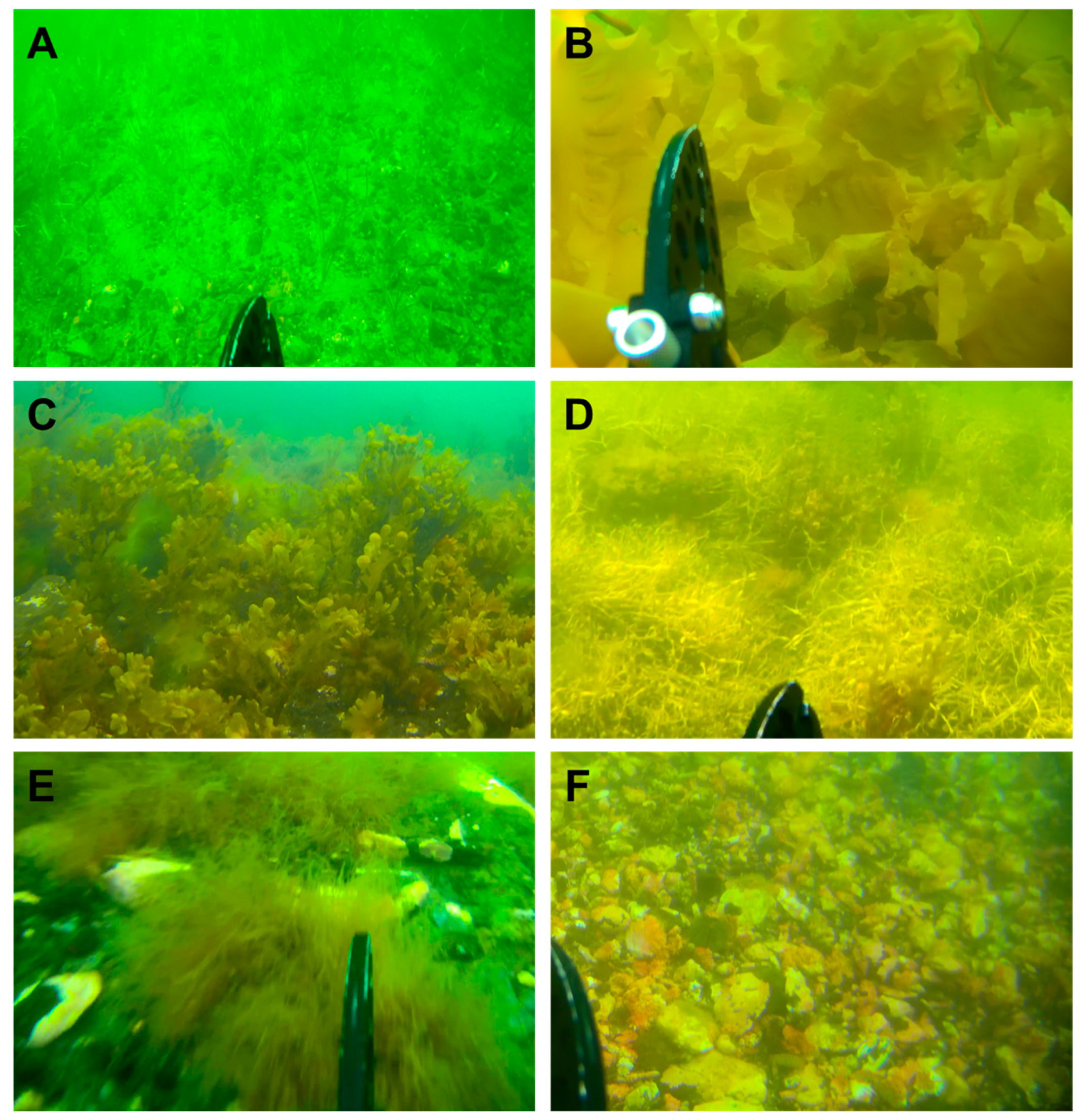
2.2.1. Underwater Survey

The underwater surveys were conducted between 5 and 8 August 2023. For this purpose, a Deep Trekker DTG3 ROV was used, which was operated from an 18-foot Crestliner Kodiac boat powered by a 40-horsepower motor. The precision of the survey was further ensured by recording coordinates using a tablet GPS system (model: T7 Tablet, Trimble Inc., Westminster, Colorado, United States). These surveys consisted of two distinct methodologies: transect (video recording) and point (imagery collection) surveys. It should be noted that videos and images were the only measurements which were collected using a camera mounted on the ROV, and there were no other measurements using ROV in this study. The transect surveys provided an overview of the habitat distribution, while the point surveys offered focused insights into specific areas of interest. The recorded data from these surveys became an essential component in the subsequent supervised classification of coastal habitats. A more detailed explanation of each survey is provided below.

Transect Survey

In the case of transect surveys, the ROV was systematically navigated along a predetermined bearing, commencing from a predefined starting location. During each 100 m transect, underwater video footage was continuously recorded. The ROV’s operational depth was typically maintained at a depth of less than 2 m above the seafloor, ensuring close proximity to the target habitats. This close range allowed for a field of view of approximately 1 m, enabling detailed and accurate documentation of the underwater environment along these transects. Transect surveys are invaluable for capturing continuous and representative data along specific paths. In summary, as illustrated in Figure 2, a total of 13 ROV transects were collected at different locations within the boundary of the study area.

Point Survey

Point surveys at 15 locations (see Figure 2) involved targeted data collection at pre-established locations of interest. The ROV was directed to these predetermined points to capture images of the seafloor. At each of these points, a number of representative images were captured. This approach is particularly useful for capturing in-depth, high-resolution data at specific points of significance, allowing for a more detailed examination of habitat characteristics, species presence, and other relevant environmental factors. Figure 3 shows several examples of the ROV imagery which were captured from different marine habitat types.

2.2.2. Multispectral Drone Survey

In total, 13 drone surveys were carried out across four study areas on 16–17 September 2023, utilizing a drone (model: Mavic 2 Enterprise Dual, SZ DJI Technology Co., Shenzhen, China). Of these surveys, four were conducted within the South Pistolet Bay and nine within the East Pistolet Bay locations (refer to Figure 2 and Figure 4). The reduced survey coverage in the South Pistolet Bay was attributed to local cabins and public access/activities that restricted the safe surveying areas.

During each flight, multispectral images (red, green, blue, and near infrared bands) were captured. All surveys were performed under light wind conditions and at a consistent flight elevation of either 70 or 100 m to enable the generation of georeferenced orthomosaic imagery. The collected imagery was overlapped (15–25% overlap per image) throughout a systematic survey path within each survey flight.

Post-processing of the drone flights was conducted using the Pix4D software, Version 1.63.0. to produce very-high-resolution orthomosaics for the four study areas, totaling approximately 1,145,000 square meters. Sample orthomosaic images are illustrated in Figure 4.

2.2.3. Shoreline Ancillary Survey

In addition to the underwater and multispectral drone surveys, shoreline ancillary surveys were conducted opportunistically in accessible areas along the shoreline of Pistolet Bay. These surveys were strategically carried out in locations that offered easy access. During these surveys, precise coordinates were recorded using a handheld GPS device (model: Geo 7X Handheld GNSS System, Trimble Inc., Westminster, Colorado, United States) to maintain accurate geospatial data. The surveyor systematically documented essential information pertaining to the shoreline environment, including photographic documentation, descriptions of shoreline habitats, identification of natural features or structures, dominant substrate analysis, and aquatic vegetation documentation. As illustrated in Figure 2, 11 and 20 exposed ancillary points were collected in August and September 2023, respectively.

2.3. Airborne Bathymetric LiDAR Data

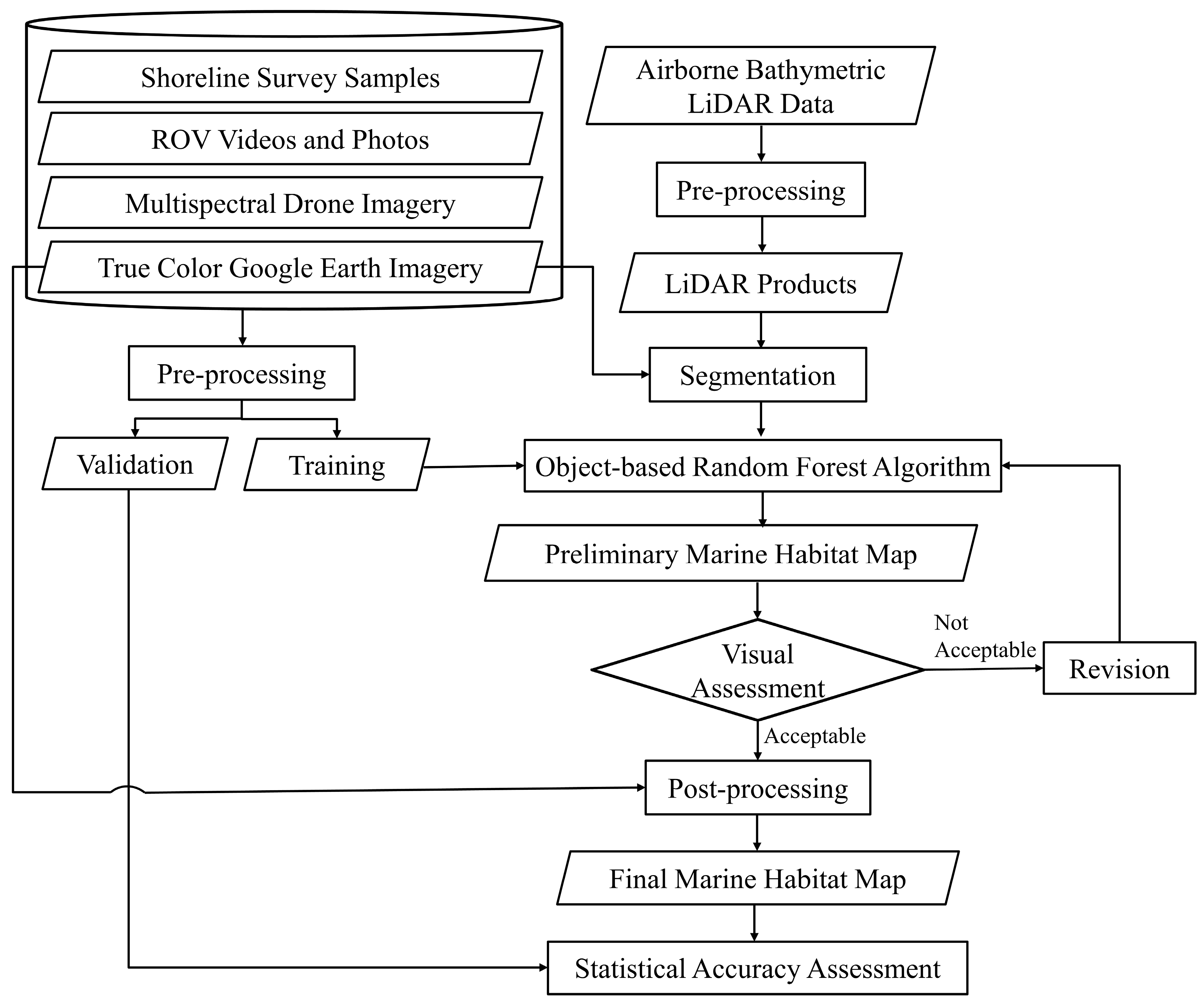
Airborne bathymetric LiDAR data were gathered by the Canadian Hydrographic Service (CHS) between mid-August and early November in 2017. The reports indicated that the accuracy in both positional data and soundings was impressively fine-tuned, with measurements boasting a precision of 0.1 m and 0.25 m, respectively.

2.4. Methodology

The framework of the RS method for marine habitat mapping in Pistolet Bay is demonstrated in Figure 5. The process of generating ground truth data polygons is explained in Section 2.4.2. This involved utilizing a combination of survey samples, ROV data, and imagery from drones and true color GE imagery. Subsequently, the preprocessed datasets were partitioned into training (70% of samples) and validation (30% of samples) sets. Additionally, LiDAR point cloud data underwent preprocessing to derive various LiDAR products (Section 2.4.3). Following this, segmentation and classification tasks were performed in the eCognition software package, Version 9.0 developed by Trimble Inc. (Westminster, Colorado, United States), utilizing both ground truth and LiDAR data (Section 2.4.4). Finally, visual and statistical accuracy assessments were carried out iteratively until the desired results were achieved (Section 2.4.5).

2.4.1. Determining Marine Habitat Classes

Initially, classes commonly found in benthic environments were categorized into two groups, surficial substrate and macroflora, and were further classified into subclasses using available literature like [25] and [NO_PRINTED_FORM] [26]. Subsequently, classes from these categories found within the study area, along with corresponding field data, were considered for classification. Further details are provided in the following subsections.

General Categorization of Classes

As mentioned earlier, the general categorization of benthic classes was conducted in the two categories of surficial substrate and macroflora. The determination of substrate composition in Pistolet Bay was carried out using the Udden-Wentworth Scale [25], a widely recognized classification system for sediment and substrate particle sizes. The substrates were categorized into specific substrate classes based on their particle size distribution, as can be seen in

Table 1. Surficial substrate categories used to categorize benthic environment.

Substrate Class	Substrate Type	Definition
Bedrock		Continuous solid bedrock
Coarse	Boulder	Rocks greater than 250 mm
	Rubble	Rocks ranging from 130 mm to 250 mm
Medium	Cobble	Rocks ranging from 30 mm to 130 mm
	Gravel	Granule size or coarser, 2 mm to 30 mm
Fine	Sand	Fine deposits ranging from 0.06 mm to 2 mm
	Mud	Material encompassing both silt and clay < 0.06 mm
Organic/Detritus		A soft material containing 85 percent or more organic materials
Shells		Calcareous remains of shellfish or invertebrates containing shells

[25].

The macroflora in Pistolet Bay were identified using established resources like [26]. The accuracy of identification was dependent on the quality of available imagery and the visibility of distinctive features. For classification purposes, the macroflora were categorized into higher-level taxonomic groups, as described in

Table 2. Macroflora categories used to classify benthic environment.

Category	Group	Species
Brown Algae	Kelp (Laminariaceae)	Agarum clathratum Alaria esculenta Laminaria digitata/Hedophyllum nigripes Saccharina lattisima
	Sourweed (Desmarestiaceae)	Desmarestia aculeata
	Brown Filamentous Algae (Phaeophyceae)
	Rockweed (Fucaceae)	Ascophyllum nodosum Fucus sp. Fucus vesiculosus
Red Algae	Coralline Algae (Corallinaceae)	Lithothamnion sp.
Seagrass	Eelgrass (Zosteraceae)	Zostera marina
Other species		Ulva sp. Ptilota sp. Green filamentous algae

.

Marine Habitat Classes Considered for Classification

Survey areas derived from both underwater transect and point surveys, as well as shoreline ancillary surveys, were systematically classified into distinct categories as part of the ground truth analysis. These categorizations were selected based on the photos and notes obtained during the field surveys. Additionally, secondary sub-categories were delineated based on the prevalent substrate class or the types of macroflora encountered (Table 1 and Table 2). This categorization process provided a structured framework for organizing and analyzing the collected data, facilitating a comprehensive assessment of the coastal habitats in Pistolet Bay.

Table 3. The primary marine habitat types identified based on the underwater and shoreline surveys data. These marine habitat classes were used in the classification model.

Primary Category	Definition
Eelgrass	Area dominated by eelgrass (>75% coverage).
Kelp	Area dominated by kelp species (>75% coverage). Substrate may not be visible. Kelp may be comprised of multiple species.
Non-Vegetation	Non-Vegetation areas with little to no flora coverage (<50%). Secondary category dependent on dominant substrate type and includes fine (mud, sand), medium (gravel, cobble), coarse (rubble, boulder), and bedrock substrates.
Other Vegetation	Areas dominated by other flora species (>75%). Secondary category describes dominant flora. Dominant substrate may vary.
Rockweed	Area dominated by rockweeds (>75% coverage). May be either dominated by Fucus sp. or Ascophyllum sp. or be a mixture of both.

provides the primary marine habitat types that were classified based on the data collected during the underwater and shoreline surveys. In fact, based on the field surveys and existing knowledge, eelgrass, kelp, and rockweed were the main vegetated marine habitat types in the study area. All other vegetated classes were considered as the Other Vegetation class.

2.4.2. Ground Truth Data Preparation

This section describes the methodology used to generate ground truth samples from underwater and shoreline survey data, visual interpretations of the drone imagery, as well as true color GE imagery and other available products.

Generating Polygons from Field Survey Data

The dominant seabed type in any area, accounting for over 50% of the coverage, was classified into one of the five distinct habitat classes mentioned in Table 3. To provide an example, training areas labeled as Non-Vegetation signify that there is less than 50% vegetation in that specific region, rather than implying an absence of vegetation altogether. As depicted in Figure 6, which is a screenshot of an ROV video captured along the 100 m transect known as A1T1 (see Figure 2), the image illustrates sparsely distributed vegetation. However, because the predominant seabed type in this area is Non-Vegetation, the associated training area derived from field data was categorized as Non-Vegetation. This approach ensures that categorizations reflect the dominant seabed type within each training area, considering the overall composition of the seabed in a particular region.

The boundary of each classified underwater and shoreline data was delineated using LiDAR intensity and GE high resolution imagery. A total of 54 polygons were generated through the interpretation of the underwater and shoreline data.

Table 4. Breakdown of ground truth polygons created from the underwater and shoreline survey data.

Class	Number of Ground Truth Polygons	Total Area (m2)
Non-Vegetation	37	516,755
Eelgrass	3	77,513
Rockweed	4	52,204
Kelp	4	72,472
Other Vegetation	6	27,043

provides a breakdown of the processed polygons, including the total area covered by each class.

Generating Polygons through Visual Interpretation of Multispectral Drone Imagery

A marine habitat specialist and an RS scientist investigated the very-high-resolution multispectral drone imagery and identified several marine habitat types by visual interpretation (see Figure 7 for an example). The boundary of each sample was then delineated, and the samples were integrated into the ArcGIS software package, Version 10.8, developed by ESRI Inc., to create the polygonal vector data. Each polygon was assigned to one of the five classes specified in Table 3. Overall, a total of 98 polygons were generated through the interpretation of the drone imagery.

Table 5. Breakdown of ground truth polygons created from the interpretation of drone imagery.

Class	Number of Ground Truth Polygons	Total Area (m2)
Non-Vegetation	39	144,859
Eelgrass	2	16,742
Rockweed	37	59,963
Kelp	0	0
Other Vegetation	20	5308

provides a breakdown of the processed polygons, including the total area covered by each class.

Generating Polygons through Visual Interpretation of True Color GE Imagery and Other Products

Similar to interpretation of very-high-resolution multispectral drone imagery, a marine habitat specialist and an RS scientist investigated the multi-temporal true color GE images collected between 2020 and 2023, assuming the locations of the marine habitat types do not change within this time frame, and several areas of marine habitat types (especially Rockweed) were identified. Overall, a total of 52 polygons were generated through the interpretation of the true color GE imagery and other products.

Table 6. Breakdown of ground truth polygons created from the interpretation of the Google Earth (GE) imagery and other products.

Class	Number of Ground Truth Polygons	Total Area (m2)
Non-Vegetation	24	382,554
Eelgrass	5	61,396
Rockweed	18	202,401
Kelp	3	38,320
Other Vegetation	2	9130

provides a breakdown of the processed polygons, including the total area covered by each class.

Total Generated Polygons

In summary, the ground truth data of marine habitat types in this study were derived from five approaches: underwater transect surveys, underwater point surveys, drone surveys, shoreline ancillary surveys, and interpretation of multi-temporal true color GE imagery and other products. All the collected data were preprocessed, converted to GIS polygon format, and consolidated in a GIS geodatabase to be used in the classification algorithms. The final GIS geodatabase of ground truth data resulted in 204 polygons, with an area of 1.67 km², the details of which are summarized in

Table 7. The total number and area of the final ground truth polygons prepared for the classification algorithm.

Class	Number of Ground Truth Polygons	Total Area (m2)
Non-Vegetation	100	1,044,167
Eelgrass	10	155,652
Rockweed	59	314,569
Kelp	7	110,792
Other Vegetation	28	41,481

. The area of the final ground truth data was approximately 1% of the total area of the study area.

The prepared ground truth polygons were the foundation for the RF algorithm in the next step of the study. These polygons were randomly divided into two groups: training (70%) and validation (30%). The training samples were used for training the classification algorithm (see Section 2.4.4) and the validation samples were used for the statistical accuracy assessment of the final habitat map (see Section 2.4.5).

2.4.3. Airborne Bathymetric LiDAR Data Processing

LiDAR data processing involved handling datasets acquired through both topographic and bathymetric lasers. Initially, a critical task involved normalizing the output from these sensors relative to each other and to the flight line to ensure a uniform LiDAR intensity across the study area. However, due to separate provisions of the two datasets, flightline artifacts persisted within the data. Following this, a comprehensive processing approach was undertaken. All *.las files underwent processing and gridding, resulting in the creation of diverse LiDAR products with a spatial resolution of 2 m. In this study, the following products were generated from the LiDAR point cloud data: water depth, Digital Surface Model (DSM), Canopy Height Model (CHM), slope, and intensity products (Figure 8). Additionally, to refine the analysis, land areas were selectively masked by employing elevation thresholding. This threshold was determined through meticulous visual analysis and was continually reassessed to ensure that no relevant areas were inadvertently included in the mask.

To derive water depth information, LiDAR point cloud data underwent classification to differentiate between seafloor points and water surface points. This classification process involved filtering out non-seafloor points, such as vegetation, using algorithms like ground filtering or hydro-flattening. Once classified, the vertical distance between the water surface and the underlying terrain could be calculated, providing accurate water depth measurements.

For generating DSM and CHM, the LiDAR point cloud data were processed to extract seafloor and vegetation points separately. Seafloor points were used to create a DSM representing the topography of the bottom of the study area, while vegetation points were utilized to generate a CHM depicting the height of vegetation above ground level. These models were created by directly gridding the LAS point elevations to a 2 m grid.

Slopes were calculated from LiDAR point cloud data by analyzing the elevation differences between neighboring points. Slope values were derived using algorithms that estimate the rate of change in elevation over a specified distance, providing insights into the steepness of terrain surfaces.

LiDAR intensity values, acquired during data acquisition, represented the strength of the reflected laser pulse and provide additional information about surface properties. It is worth noting that among the available LiDAR products in this study, intensity was the most useful data for classifying marine habitat classes because it contains different values for (1) vegetated and non-vegetated marine habitat types, and (2) different vegetated habitat types, which have different canopy structures (e.g., Kelp and Rockweed) [12].

2.4.4. Classification

After generating LiDAR products, a segmentation algorithm was applied to the LiDAR products and very-high-resolution true color GE imagery to partition the study area into coherent regions. In this study, the multi-resolution segmentation algorithm available in the eCognition software package was employed for this. The algorithm segmented the study area based on specific criteria, such as color, intensity, and texture of the input datasets [12,17,27].

In the subsequent step, the training samples along with the segmented imagery were integrated into an RF algorithm, a widely employed ensemble learning AI model for both classification and regression tasks. RF was selected because previous studies have showed the higher potential of this algorithm compared to other commonly used AI models [12,28,29]. This algorithm constructs a multitude of decision trees during the training phase and outputs the mode (for classification) or the mean (for regression) of the individual trees’ predictions. The “random” aspect is introduced by training each tree on a random subset of the training dataset and considering a random subset of features at each node in the tree-building process. This inherent randomness enhances the model’s robustness and generalization capability, thereby reducing overfitting. Renowned for its versatility and capacity to handle large datasets with high-dimensional features, RF’s aggregated predictions from multiple trees often result in a more accurate and stable model for habitat mapping [28,29,30]. The outcome of the RF algorithm constituted the preliminary marine habitat map.

2.4.5. Accuracy Assessment

The preliminary marine habitat map produced in the previous section underwent a thorough visual examination using ultra-high-resolution true color GE imagery to ensure its accuracy and to identify any significant errors. Throughout this evaluation, the parameters and input features of the RF algorithm were re-evaluated, and the classification process was iterated until visually satisfactory results were obtained. Upon achieving an acceptable level of accuracy through visual inspection, further refinement of the classification classes was undertaken through various post-processing techniques, including manual adjustments. This iterative process culminated in the production of the final marine habitat map.

Finally, a comprehensive statistical accuracy assessment was performed to validate the precision of the final marine habitat map (see Figure 9). To this end, a confusion matrix of the classification was created using the validation samples, and different accuracy measures, including Overall Accuracy (OA), Producer’s Accuracy (PA), and User’s Accuracy (UA), and Cohen’s Kappa Coefficient (KC) [31], were assessed.

3. Results

Figure 9 illustrates the outcome of the marine habitat classification conducted in Pistolet Bay, along with two specific zoomed regions. Upon visually analyzing these maps and cross-referencing them with highly detailed true color GE imagery, it was observed that the identified zones closely aligned with the actual habitat types within the study area. For instance, deep regions were accurately classified as non-vegetated, and areas designated as Rockweed corresponded correctly with rocky terrain. Additionally, segments identified as Eelgrass exhibited a distinct greenish hue in the water, which is typically associated with eelgrass beds.

The area of each class was calculated utilizing the generated map, and the comprehensive findings are presented in

Table 8. Area of each marine habitat class obtained from the produced map.

Class	Area (km2)	Percentage Area (%)
Rockweed	17.89	11.09
Kelp	36.93	22.89
Other Vegetation	14.64	9.07
Eelgrass	16.65	10.32
Non-Vegetation	75.23	46.63

. It is evident from the analysis that Non-Vegetation occupied 46.63% of the study area, while vegetated habitats, including Rockweed, Kelp, Eelgrass, and Other Vegetation, covered the remaining 53.37%. Non-vegetated areas may be characterized by deeper water depths or substrate types that are unsuitable for the attachment or growth of vegetation. Non-vegetated areas could include sandy bottoms, rocky outcrops, or regions with strong currents that prevent the establishment of plant life. As mentioned previously, non-vegetated areas might be also indicative of sparsely vegetated areas.

The accuracy of the produced marine habitat map was also statistically assessed using the confusion matrix, the results of which are provided in

Table 9. The confusion matrix of the marine habitat map (OA, KC, PA, UA, OE, and CE stand for Overall Accuracy, Kappa Coefficient, Producer Accuracy, User Accuracy, Omission Error, and Commission Error, respectively).

Mapped Class	Ground Truth Validation Sample
		Rockweed	Kelp	Other Vegetation	Eelgrass	Non-Vegetation	Row Total	UA (%)	CE (%)
	Rockweed	55,200	0	88	70	8183	63,541	86.87	13.13
	Kelp	0	30,499	0	0	42	30,541	99.86	0.14
	Other Vegetation	974	0	333	747	107	2161	15.41	84.59
	Eelgrass	77	0	0	80,601	250	80,928	99.60	0.40
	Non-Vegetation	24,318	754	11	8775	185,577	219,435	84.57	15.43
	Column Total	80,569	31,253	432	90,193	194,159	396,606
	PA (%)	68.51	97.59	77.08	89.37	95.57
	OE (%)	31.49	2.41	22.92	10.63	4.43		OA = 88.81% KC = 0.83

. This confusion matrix provides a comprehensive overview, aiding in understanding the model’s strengths and weaknesses across specific vegetation classes. The overall classification accuracy was 88.81%, indicating the high potential of the developed RS model for discriminating the marine habitat types in the study area. This level of overall accuracy simply means that if we randomly select 100 points (each having a size of 5 × 5 m) considering all classes, 89 of them would be correctly identified within the produced map.

The PA and UA for each class are also provided in Table 7. Overall, based on both the PAs and UAs, Kelp (PA = 97.59%, UA = 99.86%), Eelgrass (PA = 89.37%, UA = 99.60%), and Non-Vegetation (PA = 95.57%, UA = 84.57%) had the highest classification accuracies. For example, 30,499 pixels out of 31,253 pixels of the Kelp samples were correctly classified as Kelp. Among all the classes, the UA for the Other Vegetation class was considerably low (15.41%). The main reason was that some samples of Rockweed and Eelgrass were wrongly classified as Other Vegetation. Moreover, the Non-Vegetation class is a general category which could include various classes such as sand or rock, which may have different responses in RS products.

4. Discussion

Despite the efforts made in achieving high classification accuracy, the study encountered several challenges that underscore the need for continued research and refinement. One notable limitation lies in the broad categorization of the Non-Vegetation class, which encompasses a diverse array of substrates in terms of their sizes, such as sand (on the order of mm) or rock (on the order of cm). Each substrate type may present unique spectral responses in remote sensing products, complicating the accurate classification of non-vegetated areas. For example, while sandy bottoms may exhibit relatively uniform spectral signatures, rocky outcrops could display considerable spectral heterogeneity due to variations in mineral composition and surface roughness. Consequently, the indiscriminate grouping of these disparate substrates under the Non-Vegetation class may lead to misclassifications and inaccuracies in habitat mapping efforts.

Although a diverse range of resources were utilized in this study to generate ground truth samples for training the classification algorithm, it became evident that certain habitat classes, notably Eelgrass and Kelp, were underrepresented in the sample dataset. With only 10 ground truth samples for Eelgrass and 7 for Kelp, the limited sample size posed a challenge to the robustness and generalizability of the developed algorithm. Insufficient representation of these critical habitat types may lead to biases in the model’s classification outcomes and compromise the accuracy of habitat mapping efforts. Therefore, addressing this limitation is imperative to ensure the reliability and effectiveness of the classification model in accurately delineating marine habitats.

Within the spectrum of vegetated marine habitats, kelp stood out as the dominant feature, encompassing a significant portion of the study area at 36.93 square km. The prevalence of kelp-dominated areas suggests favorable conditions such as shallow waters with ample sunlight penetration, nutrient-rich waters, and suitable substrates for kelp attachment [32]. Kelp forests often thrive in areas with moderate wave action and provide essential habitats for various marine species. On the other hand, Rockweed, Eelgrass, and Other Vegetation each contributed approximately 10% (16 square km) to the total area under consideration. The distribution of these vegetated habitats may be influenced by factors such as substrate composition, water depth, salinity levels, and tidal influence. Rockweed typically thrives in intertidal zones, clinging to rocky substrates, while eelgrass beds prefer shallow, sheltered areas with soft sediment [33,34]. Overall, the distribution of these habitat types reflects the complex interactions between the physical, chemical, and biological factors within the marine environment.

It was observed that leveraging emerging technologies such as multispectral drone imagery presents a promising solution for marine habitat mapping. Drones equipped with high-resolution multispectral cameras can capture detailed imagery of coastal and underwater habitats with unprecedented spatial and temporal resolution. Moreover, drone imagery offers distinct advantages over traditional field-based methods, including the ability to access remote or inaccessible areas, cover large spatial extents efficiently, and capture fine-scale habitat features with high fidelity.

As discussed, the airborne bathymetric LiDAR data were the main source of data for classifying the marine habitats in this study. There were several reasons for selecting this data, including (1) the study area was relatively large (170 km²) and utilizing other datasets, such as drone imagery or shipborne Sound Navigation and Ranging (SONAR) data, was not feasible and cost-effective [7]; (2) the study area was relatively shallow water (i.e., up to −28 m) and, thus, airborne bathymetric LiDAR data were an optimal option because LiDAR has a penetration up to approximately 30 m depending on the turbidity and quality of the water [10,11,35]; and (3) a variety of products, such as intensity, DEM, and CHM can be derived from LiDAR data, each of which can identify specific characteristics of habitat types and, thus, could beneficial for discriminating different habitat types.

Furthermore, it is crucial to recognize the multifaceted influence of environmental factors on the accuracy of habitat classification models. Factors such as water turbidity, which refers to the cloudiness or haziness of water caused by suspended particles, can significantly impact the spectral reflectance of underwater features. Likewise, seasonal variations in environmental conditions, such as changes in water temperature, light availability, and biological productivity, can induce temporal fluctuations in habitat characteristics. For instance, the phenological cycles of marine vegetation, such as eelgrass or kelp, may exhibit distinct spectral signatures during different seasons, necessitating seasonal calibration and validation of classification models to account for temporal variability.

In addition to environmental factors, sensor limitations also play a pivotal role in shaping the accuracy and reliability of habitat classification models. For example, the airborne bathymetric LiDAR data utilized in this study exhibited various errors, including prominent flight line artifacts, which posed significant challenges to the accuracy and reliability of the data. Despite diligent efforts to mitigate these errors through post-processing techniques, certain inaccuracies persisted, ultimately impacting the outcomes of the study. Flight line artifacts, in particular, are inherent to the data acquisition process and can arise from factors such as sensor misalignment, inconsistent data collection intervals, or discrepancies in laser pulse densities along flight lines. These persistent errors introduced uncertainties and biases into the dataset, consequently influencing the analysis and interpretation of the study results. For instance, flight line artifacts may manifest as irregularities in elevation or intensity values, leading to distortions in terrain modeling and habitat classification efforts. Moreover, the presence of these errors can undermine the accuracy of the derived LiDAR products and compromise the reliability of subsequent analyses, thereby diminishing the overall robustness of the study outcomes. Future studies may benefit from exploring alternative data acquisition methods or integrating complementary datasets to mitigate the impact of inherent errors and enhance the accuracy of LiDAR-based analyses.

In summary, while the current study achieved commendable results in marine habitat classification, addressing the identified limitations and incorporating suggested improvements will be crucial for advancing the accuracy and applicability of remote sensing-based habitat mapping in marine environments.

5. Conclusions

The objective of the current study was marine habitat mapping in Pistolet Bay, Newfoundland, Canada, using various RS datasets and an RF algorithm. The datasets utilized in this study encompassed diverse ground surveying data alongside airborne bathymetric LiDAR data. Ground truth surveys employed a multifaceted approach, including underwater surveys using ROV video and images, multispectral drone surveys, and shoreline ancillary surveys. A multi-resolution segmentation algorithm along with an RF classification algorithm were applied to the dataset to produce the marine habitat map after several post-processing steps. A visual analysis of the classification maps demonstrated the effectiveness of the classification model in accurately delineating various habitat types. Notably, non-vegetated areas comprised 46.63% of the study area, with vegetated habitats covering the remaining 53.37%. Kelp emerged as the dominant habitat type, encompassing 36.93 square km, indicative of favorable environmental conditions such as shallow waters and ample sunlight penetration. Despite the overall high classification accuracy of 88.81%, challenges, such as limited ground truth samples for certain habitat classes and inherent errors in the LiDAR data, such as flight line artifacts, were encountered. These limitations underscore the need for continued research efforts to refine classification models and address data uncertainties. Finally, considering the high potential of the developed classification algorithm, it is suggested to apply it to marine habitat mapping in all shallow water bodies (i.e., less than 30 m water depth) in Newfoundland’s coastal areas to obtain up-to-date information about the coverage and status of marine habitats in the province.

References

1. Klemas, V. Remote sensing of coastal and ocean currents: An overview. J. Coast. Res. 2012, 28, 576–586. [Google Scholar]
2. Rani, M.; Seenipandi, K.; Rehman, S.; Kumar, P.; Sajjad, H. Remote Sensing of Ocean and Coastal Environments; Elsevier: Amsterdam, The Netherlands, 2020. [Google Scholar]
3. Koch, E.W. Beyond light: Physical, geological, and geochemical parameters as possible submersed aquatic vegetation habitat requirements. Estuaries 2001, 24, 1–17. [Google Scholar] [CrossRef]
4. Klemas, V.V. Remote sensing of submerged aquatic vegetation. In Seafloor Mapping along Continental Shelves: Research and Techniques for Visualizing Benthic Environments; Springer: Cham, Switzerland, 2016; pp. 125–140. [Google Scholar]
5. Rowan, G.; Kalacska, M. Remote sensing of submerged aquatic vegetation: An introduction and best practices review. Preprints 2020. [Google Scholar] [CrossRef]
6. Amani, M.; Ghorbanian, A.; Asgarimehr, M.; Yekkehkhany, B.; Moghimi, A.; Jin, S.; Naboureh, A.; Mohseni, F.; Mahdavi, S.; Layegh, N.F. Remote sensing systems for ocean: A review (Part 1: Passive systems). IEEE J. Sel. Top. Appl. Earth Obs. Remote Sens. 2021, 15, 210–234. [Google Scholar] [CrossRef]
7. Amani, M.; Mohseni, F.; Layegh, N.F.; Nazari, M.E.; Fatolazadeh, F.; Salehi, A.; Ahmadi, S.A.; Ebrahimy, H.; Ghorbanian, A.; Jin, S.; et al. Remote sensing systems for ocean: A review (part 2: Active systems). IEEE J. Sel. Top. Appl. Earth Obs. Remote Sens. 2022, 15, 1421–1453. [Google Scholar] [CrossRef]
8. Li, X.; Liu, B.; Zheng, G.; Ren, Y.; Zhang, S.; Liu, Y.; Gao, L.; Liu, Y.; Zhang, B.; Wang, F. Deep-learning-based information mining from ocean remote-sensing imagery. Natl. Sci. Rev. 2020, 7, 1584–1605. [Google Scholar] [CrossRef] [PubMed]
9. McCarthy, M.J.; Colna, K.E.; El-Mezayen, M.M.; Laureano-Rosario, A.E.; Méndez-Lázaro, P.; Otis, D.B.; Toro-Farmer, G.; Vega-Rodriguez, M.; Muller-Karger, F.E. Satellite remote sensing for coastal management: A review of successful applications. Environ. Manag. 2017, 60, 323–339. [Google Scholar] [CrossRef] [PubMed]
10. Hostetler, C.A.; Behrenfeld, M.J.; Hu, Y.; Hair, J.W.; Schulien, J.A. Spaceborne lidar in the study of marine systems. Ann. Rev. Mar. Sci. 2018, 10, 121–147. [Google Scholar] [CrossRef] [PubMed]
11. Le Quilleuc, A.; Collin, A.; Jasinski, M.F.; Devillers, R. Very high-resolution satellite-derived bathymetry and habitat mapping using pleiades-1 and ICESat-2. Remote Sens. 2021, 14, 133. [Google Scholar] [CrossRef]
12. Amani, M.; Macdonald, C.; Salehi, A.; Mahdavi, S.; Gullage, M. Marine Habitat Mapping Using Bathymetric LiDAR Data: A Case Study from Bonne Bay, Newfoundland. Water 2022, 14, 3809. [Google Scholar] [CrossRef]
13. Conti, L.A.; da Mota, G.T.; Barcellos, R.L. High-resolution optical remote sensing for coastal benthic habitat mapping: A case study of the Suape Estuarine-Bay, Pernambuco, Brazil. Ocean. Coast. Manag. 2020, 193, 105205. [Google Scholar] [CrossRef]
14. Brock, J.C.; Purkis, S.J. The emerging role of lidar remote sensing in coastal research and resource management. J. Coast. Res. 2009, 1–5. [Google Scholar] [CrossRef]
15. Pe’eri, S.; Long, B. LIDAR technology applied in coastal studies and management. J. Coast. Res. 2011, 1–5. [Google Scholar] [CrossRef]
16. Monteiro, J.G.; Jiménez, J.L.; Gizzi, F.; Přikryl, P.; Lefcheck, J.S.; Santos, R.S.; Canning-Clode, J. Novel approach to enhance coastal habitat and biotope mapping with drone aerial imagery analysis. Sci. Rep. 2021, 11, 574. [Google Scholar] [CrossRef] [PubMed]
17. Ventura, D.; Bonifazi, A.; Gravina, M.F.; Belluscio, A.; Ardizzone, G. Mapping and classification of ecologically sensitive marine habitats using unmanned aerial vehicle (UAV) imagery and object-based image analysis (OBIA). Remote Sens. 2018, 10, 1331. [Google Scholar] [CrossRef]
18. Ventura, D.; Grosso, L.; Pensa, D.; Casoli, E.; Mancini, G.; Valente, T.; Scardi, M.; Rakaj, A. Coastal benthic habitat mapping and monitoring by integrating aerial and water surface low-cost drones. Front. Mar. Sci. 2023, 9, 1096594. [Google Scholar] [CrossRef]
19. Greene, H.G. Habitat characterization of a tidal energy site using an ROV: Overcoming difficulties in a harsh environment. Cont. Shelf Res. 2015, 106, 85–96. [Google Scholar] [CrossRef]
20. Macreadie, P.I.; McLean, D.L.; Thomson, P.G.; Partridge, J.C.; Jones, D.O.; Gates, A.R.; Benfield, M.C.; Collin, S.P.; Booth, D.J.; Smith, L.L.; et al. Eyes in the sea: Unlocking the mysteries of the ocean using industrial, remotely operated vehicles (ROVs). Sci. Total Environ. 2018, 634, 1077–1091. [Google Scholar] [CrossRef]
21. McLean, D.L.; Parsons, M.J.; Gates, A.R.; Benfield, M.C.; Bond, T.; Booth, D.J.; Bunce, M.; Fowler, A.M.; Harvey, E.S.; Macreadie, P.I.; et al. Enhancing the scientific value of industry remotely operated vehicles (ROVs) in our oceans. Front. Mar. Sci. 2020, 7, 220. [Google Scholar] [CrossRef]
22. Da Silveira, C.B.L.; Strenzel, G.M.R.; Maida, M.; Gaspar, A.L.B.; Ferreira, B.P. Coral reef mapping with remote sensing and machine learning: A nurture and nature analysis in marine protected areas. Remote Sens. 2021, 13, 2907. [Google Scholar] [CrossRef]
23. Papachristopoulou, I.; Filippides, A.; Fakiris, E.; Papatheodorou, G. Vessel-based photographic assessment of beach litter in remote coasts. A wide scale application in Saronikos Gulf, Greece. Mar. Pollut. Bull. 2020, 150, 110684. [Google Scholar] [CrossRef] [PubMed]
24. ParksNL. Pistolet Bay Provincial Park. Available online: https://www.parksnl.ca/parks/pistolet-bay-provincial-park/ (accessed on 20 July 2022).
25. Wentworth, C.K. A scale of grade and class terms for clastic sediments. J. Geol. 1922, 30, 377–392. [Google Scholar] [CrossRef]
26. Gosner, K.L. A Field Guide to the Atlantic Seashore: From the Bay of Fundy to Cape Hatteras; Houghton Mifflin Harcourt: Boston, MA, USA, 1999; Volume 24. [Google Scholar]
27. Janowski, L.; Wroblewski, R.; Dworniczak, J.; Kolakowski, M.; Rogowska, K.; Wojcik, M.; Gajewski, J. Offshore benthic habitat mapping based on object-based image analysis and geomorphometric approach. A case study from the Slupsk Bank, Southern Baltic Sea. Sci. Total Environ. 2021, 801, 149712. [Google Scholar] [CrossRef] [PubMed]
28. Amani, M.; Salehi, B.; Mahdavi, S.; Granger, J.E.; Brisco, B.; Hanson, A. Wetland classification using multi-source and multi-temporal optical remote sensing data in Newfoundland and Labrador, Canada. Can. J. Remote Sens. 2017, 43, 360–373. [Google Scholar] [CrossRef]
29. McLaren, K.; McIntyre, K.; Prospere, K. Using the random forest algorithm to integrate hydroacoustic data with satellite images to improve the mapping of shallow nearshore benthic features in a marine protected area in Jamaica. GIsci. Remote Sens. 2019, 56, 1065–1092. [Google Scholar] [CrossRef]
30. Wicaksono, P.; Aryaguna, P.A.; Lazuardi, W. Benthic habitat mapping model and cross validation using machine-learning classification algorithms. Remote Sens. 2019, 11, 1279. [Google Scholar] [CrossRef]
31. Cohen, J. A coefficient of agreement for nominal scales. Educ. Psychol. Meas. 1960, 20, 37–46. [Google Scholar] [CrossRef]
32. Randell, Z.; Kenner, M.; Tomoleoni, J.; Yee, J.; Novak, M. Kelp-forest dynamics controlled by substrate complexity. Proc. Natl. Acad. Sci. USA 2022, 119, e2103483119. [Google Scholar] [CrossRef] [PubMed]
33. Mathieson, A.C.; Dawes, C.J. Seaweeds of the Northwest Atlantic; University Massachusetts Press: Amherst, MA, USA, 2017. [Google Scholar]
34. Eriander, L.; Infantes, E.; Olofsson, M.; Olsen, J.L.; Moksnes, P.-O. Assessing methods for restoration of eelgrass (Zostera marina L.) in a cold temperate region. J. Exp. Mar. Biol. Ecol. 2016, 479, 76–88. [Google Scholar] [CrossRef]
35. Pratomo, D.G.; Putranto, B.F.E. Analysis of the green light penetration from Airborne LiDAR Bathymetry in Shallow Water Area. IOP Conf. Ser. Earth Environ. Sci. 2019, 389, 012003. [Google Scholar] [CrossRef]
Figure 1. (a) Pistolet Bay’s position (indicated with the purple color) at the northern tip of Newfoundland Island, Canada, and (b) the boundary of the study area is enclosed with the purple line.
Remotesensing 16 02654 g001
Figure 2. Ground truth survey types and locations in Pistolet Bay.
Remotesensing 16 02654 g002
Figure 3. Frequently observed marine habitat types (A) eelgrass, (B) sugar kelp, (C) rockweed Fucus sp., (D) rockweed Ascophyllum nodosum, (E) brown filamentous algae, and (F) crustose coralline algae in the ROV point surveys.
Remotesensing 16 02654 g003
Figure 4. (ad) The generated true color drone orthomosaics from four locations in Pistolet Bay. The locations of these images are indicated with D1 to D4 in Figure 2, respectively. The purple lines in the figures indicate the waterline.
Remotesensing 16 02654 g004
Figure 5. Flowchart of the proposed remote sensing method for marine habitat mapping.
Remotesensing 16 02654 g005
Figure 6. A screenshot of an ROV video from one of the transects (A1T1, indicated by the red line), showing an area that was considered Non-Vegetation despite presence of sparse vegetation. The purple curve indicates the waterline in the study area.
Remotesensing 16 02654 g006
Figure 7. (a) True color drone imagery showing exposed (orange) and submerged (green) rockweed; (b) the location of rockweed derived from filtering the drone imagery; (c) the final boundary of the rockweed (cyan line) delineated manually using the imagery.
Remotesensing 16 02654 g007
Figure 8. The products derived from airborne bathymetric LiDAR point cloud data. (a) Water depth, (b) Digital Surface Model (DSM), (c) Canopy Height Model (CHM), (d) slope, and (e) intensity.
Remotesensing 16 02654 g008
Figure 9. The final produced marine habitat map over the study area along with two zoomed areas and their corresponding classified maps.
Remotesensing 16 02654 g009