An Effective Scheme for Modeling and Compensating Differential Age Errors in Real-Time Kinematic Positioning

Abstract

In many real-time kinematic (RTK) positioning applications, reference observations are transmitted over wireless links that can experience frequent interruptions or substantial delays. This results in large differential ages between base and rover observations, which, in turn, leads to a deterioration in positioning performance. To bridge the significant age difference, in this work, we propose a simple and effective scheme for modeling and compensating for such errors. Firstly, the overall differential age error was modeled using truncated Taylor expansion. Then, a time-differenced carrier phase (TDCP)-based observation model was established to estimate the errors with the Kalman framework. Since estimating the receiver’s clock error is unnecessary, equivalent transformation and sequential filtering technology were adopted to significantly reduce the computational complexity. Furthermore, a predictor performance monitor was introduced to mitigate the integrity risks that may occur due to model mismatches. The effectiveness of this scheme was validated by static and dynamic field experiments. The static experiment results showed that when the differential age was 60 s, the GPS and BDS satellites’ overall root mean square error (RMSE) with the asynchronous RTK (ARTK) prediction method was 2.8 and 5.5 times that of the proposed method, respectively. Moreover, when the differential age was 120 s, these values were 3.3 and 5.4 times that of the proposed method, respectively. The field experiment results showed that when the differential age was 60 s, the integer ambiguity fixed rate and false fixed rate of the ARTK method were 0.90 and 1.63 times that of the proposed method, respectively. Finally, at a 120 s differential age, these values were 0.78 and 4.78 times that of the proposed, respectively.

1. Introduction

The real-time kinematic (RTK) technique based on the Global Navigation Satellite System (GNSS) has unique advantages, such as high precision, fast initialization, and excellent adaptability [1,2,3]. It is used in many fields, such as autonomous driving, unmanned aerial vehicles, precision agriculture, and smart robot navigation [4,5,6,7]. In ideal conditions, the observations of the base station and the rover at the same epoch must be obtained to completely eliminate various error terms; otherwise, the positioning performance may deteriorate. In most practical real-time applications, the base station data are transferred via wireless communication. For example, in the widely used network RTK (NRTK) technique for autonomous driving applications, the observations are broadcast using a cellular mobile communication network [8]. However, due to the inherent uncertainty of the radio propagation environment, uncertainty, delays, or interruptions occur when transmitting base station observations to the rover station [9,10,11]. Hence, the time asynchrony between the observations of the base station and the rover station is inevitable. This is called the differential age, and its practical value can range from less than one second to dozens of seconds [11], sometimes even reaching hundreds of seconds. In this context, it is challenging to ensure that RTK solutions meet the high-continuity, reliability, and precision position requirements of high-dynamic applications.

The most common method is to use the base station’s historical observations and the latest rover observations directly for RTK processing [12,13,14,15,16]. This is referred to as the asynchronous RTK (ARTK) technique. These methods assume that the differential age is small and simply ignore the errors caused by a large differential age. Therefore, as the differential age increases, errors, such as satellite ephemeris, and clock and atmospheric errors, dramatically increase, resulting in a rapid decrease in positioning accuracy. In [15], the errors caused by the differential age using the ARTK method, such as those mentioned above, are theoretically analyzed. It is shown that satellite ephemeris errors are the main factors affecting the ARTK method’s positioning accuracy during the ionospheric inactivity season. This study also demonstrates that ARTK positioning accuracy deterioration is usually negligible within a 0.5 s differential age, and centimeter-level accuracy can be achieved within a 15 s differential age. Using the above theoretical analysis, these errors are further analyzed based on experimental data spanning one month in [16]. This work shows that, due to the small change in broadcast ephemeris errors, the ARTK performance of BDS and Galileo is generally better than that of GPS and GLONASS with large differential ages. In addition, it is demonstrated that ionospheric errors are usually the more dominant factor, and during active ionospheric conditions, they can reach several centimeters with a 15 s latency.

Besides ARTK methods, several methods have been proposed to predict missing reference observations under large differential ages. The patent described in [17] uses a least-square-based time-polynomial fitting method to predict the reference station carrier phase in kinematic applications, in which the previous 7 s phase observations are used to predict the following 10 s carrier phase. The calculation results showed that the prediction accuracy for a 10 s differential age was approximately 11 cm. The idea behind this method is relatively straightforward, but the prediction accuracy is limited. To predict reference observations with larger differential ages, a method based on ultra-rapid precision ephemeris products is proposed in [18]. In this method, the ultra-rapid precision ephemeris is utilized to eliminate most of the satellite orbit and clock errors; then, atmospheric errors are mitigated by employing the Saatamoinen model and dual-frequency observations. The proposed approach can achieve centimeter-level accuracy with as much as a 15 min differential age. However, this method requires ultra-rapid precision ephemeris and dual-frequency observations, making it unsuitable for low-cost or single-frequency GNSS receiver applications. Based on the strong temporal and spatial correlations between geosynchronous earth orbit (GEO) satellite observations, an algorithm is proposed to predict interrupted GEO satellite observations with the minimum mean squared error criterion for the BDS system [19]. The test results show that this method can still achieve millimeter-level accuracy with a minute-level differential age. However, this method only targets a few BDS GEO satellites. Moreover, the number of visible GEO satellites is sometimes very low for highly dynamic applications, and, in such cases, the RTK performance drops significantly.

As mentioned above, the differential age error is composed of multiple components, such as orbit, clock, and atmospheric errors. An alternative option is to model and predict these errors separately [20,21,22,23]. However, such research usually focuses on precise-point-positioning real-time kinematic (PPP-RTK) [24,25] applications. As the system architecture of a typical PPP-RTK application is vastly different from that of a traditional RTK system based on DD observations, these methods are not directly suitable for the applications discussed in this work. Nonetheless, a special form of PPP-RTK systems, the single-station PPP-RTK system [26,27], is comparable to the traditional RTK technology discussed in this article. Similar to traditional RTK systems, only one reference base station is required, and the state-space representation (SSR) corrections of the PPP-RTK system can be easily converted into observation-space representation (OSR) observations [28]. After such a conversion, the following processing is identical to that of the traditional DD observations-based RTK algorithm. Since these methods essentially parameterize the errors in the time domain, they usually exhibit good robustness to large correction ages [27,29]. However, since in this type of method, various errors, such as orbit, clock, and atmosphere errors, need to be separated and estimated from observations, it usually requires a relatively long convergence time. For example, the complete convergence of the estimation takes dozens of minutes in the experiment presented in [26]. Unlike traditional RTK systems, an accurate position solution cannot be obtained immediately after acquiring the observations from the reference station.

In summary, the performance degradation caused by a large differential age is a broad issue, and the above existing methods all have specific limitations or constraints. Based on the Kalman filter framework, in this work, we propose a differential age error estimation and compensation scheme. Firstly, based on the carrier phase observation model, the error structure of the DD observation measurement caused by the differential age was analyzed. Then, we performed Taylor expansion of the differential age error and used first-order terms to model it. Based on this model, we constructed a TDCP-based (time-differenced carrier phase) observation model and state transition for Kalman estimation. Since the receiver’s clock error fluctuations do not need to be estimated, the Kalman estimator was subsequently reconstructed using equivalent transformation [30,31], and sequential filtering technology was adopted to greatly reduce the computational complexity.

Additionally, a predictor performance monitor was designed to mitigate system integrity risks. Finally, a 24 h static experiment and a dynamic field experiment were conducted. The static experiment verified the effectiveness of the proposed estimation and compensation method for differential age errors, while the dynamic field experiment validated the proposed method’s improvement in RTK positioning performance in real dynamic scenarios.

The main contributions of this paper are as follows:

(1)

A novel scheme for estimating and compensating for the differential age error in the RTK algorithm is proposed. Both static and dynamic field experiments verified the effectiveness of the proposed method, and the probability of obtaining fixed RTK solutions was significantly increased in a scenario with a relatively large differential age (e.g., 120 s);

(2)

A predictor performance monitor based on historical base station observation data was designed. An alert is issued when there is a statistical deviation between the predicted and the actual error. This serves as input for subsequent integrity assessments and helps mitigate system risks;

(3)

The proposed scheme adopts the equivalent transformation method to reduce the dimension of the Kalman filter state vector and further utilizes sequential filtering technology, significantly enhancing the computational efficiency of error model estimation.

This paper is organized as follows. Section 2.1 introduces the differential age error from the carrier phase observation equation. Section 2.2 presents the proposed differential age error model estimation and compensation scheme in detail. The predictor performance monitor is outlined in Section 2.2.4. Thereafter, the static and kinematic experiments and their results are described in Section 3, and the discussion is presented in Section 4. In Section 5, the summaries and conclusions are given. The notations used in the paper are listed in Table 1.

Table 1. Notations used in this paper.

Notations	Description
${(.)}^i$/${(.)}_b$/${(.)}_r$/${(.)}_{br}$	variable of satellite i/base/rover/(difference between base and rover)
$\nabla \Delta (.)$	double difference(DD) operation between base/rover receivers and satellites
c/$\varphi$/$\rho$	speed of light/carrier phase observation/distance between satellite and receiver
$I^i$/$T^i$	ionosphere/troposphere delay for satellite i
$d{t}_b$/$d{t}^i$	clock offset of base receiver/satellite i
${\delta }_b$/${\delta }^i$	hardware carrier phase delay of receiver (base)/satellite i
$o^i$	satellite orbit error of satellite i
${\varphi }_b$/${\varphi }^i$	receiver (base)/satellite i initial phase
$\lambda$, $N^i$	carrier phase wavelength, and integer ambiguity
${\alpha }^i$	the coefficient of the proposed model, superscript i denotes satellite i
${\sigma }_b^i$, ${\tilde{\sigma }}^i$	undifferentiated carrier phase and TDCP noise of satellite i
${\epsilon }^i$/${\epsilon }_{rb}^{ij}$	undifferentiated/double differentiated observation noise
$e_{age}^{ij}$	differential age error between satellites i and j
$v_{\varphi }^i$	observed-minus-computed (OMC) of undifferentiated carrier phase of satellite i
$r_{tdcp}^i$, ${\tilde{\epsilon }}^i$	TDCP ratio, and its observation noise
${\eta }_r$, $n_{{\eta }_r}$	the receiver clock fluctuation ratio, and its process noise
${\xi }^i$, $n_{\alpha }^i$	correlation time and process noise of the model coefficient ${\alpha }^i$
$q^i$, $q_r$	the variance of process noise $n_{\alpha }^i$ and $n_{{\eta }_r}$
L	The number of carrier phase observations
$\mathit{x}$,${\mathit{x}}^{\prime }$	state vector before and after equivalent transformation
${\mathit{x}}^{-}$	the predicted state vector in Kalman filter
$\mathit{A}$, $\mathit{F}$	state transition matrix, and its differential matrix in Kalman filter
$\mathit{Q}$, $\mathit{R}$	the process noise covariance matrix, and observation noise covariance matrix
$\mathit{H}$, $\mathit{M}$	observation matrix before, and after equivalent transformation
$\mathit{P}$,${\mathit{P}}^{-}$	covariance matrix of the state vector, and the predicted version in Kalman filter
$\mathit{z}$, $\mathit{K}$	the observation vector and the Kalman gain in Kalman filter
${\widehat{e}}_{age}^{ij}$, ${\widehat{\mathit{e}}}_{\mathit{age}}$	the estimated differential age error and its vector form
${\mathit{e}}_{\Delta \tau }$, ${\widehat{\mathit{e}}}_{\Delta \tau }$	the calculated and estimated prediction error
${\mathsf{\Omega }}_{dd},{\widehat{\mathsf{\Omega }}}_{dd}$	the original and compensated DD observation’s covariance matrix
$\mathbf{\Gamma }$	the statistic of the performance monitor
${\tau }_{age}$	the assumed differential age in the experiment section

2. Materials and Methods

2.1. Carrier Phase Observation Equation

The carrier phase observation equation of satellite i at time t is given as follows [32]:

$${\varphi }_b^i\left(t\right)={\rho }_b^i-I^i\left(t\right)+T^i\left(t\right)+c(d{t}_b\left(t\right)-d{t}^i\left(t\right))+{\delta }_b+{\delta }^i+o^i\left(t\right)+\lambda ({\varphi }_b+{\varphi }^i+{\overline{N}}^i)+{\epsilon }_b^i$$

(1)

where the subscript b denotes the base station, and in the following text, the subscript r denotes the rover. In addition, ${\varphi }_b^i\left(t\right)$ is the carrier phase observation of satellite i at time t, in meters; ${\rho }_b^i$ denotes the distance between the phase center of the satellite antenna and the phase center of the GNSS receiver (base) antenna in meters; $I^i\left(t\right)$ and $T^i\left(t\right)$ represent the ionosphere delay and troposphere delay at time t in meters, respectively; $d{t}_b\left(t\right)$ and $d{t}^i\left(t\right)$ denote the receiver (base) clock offset and satellite clock offset at time t in seconds; ${\delta }_b$ and ${\delta }^i$ represent the receiver and satellite carrier phase hardware delay in meters, respectively; $o^i\left(t\right)$ is the error of satellite orbit at time t in meters; ${\varphi }_b$ and ${\varphi }^i$ denote the initial phase of the receiver and satellite i in cycles; $\lambda$ is the carrier phase wavelength in meters/cycle; and $N^i$ is the carrier integer ambiguity in cycles.

As shown in Figure 1, the DD operation is usually conducted to eliminate various uncertainty errors for the RTK algorithm [33]:

$$\begin{array}{cc}\hfill \nabla \Delta {\varphi }_{rb}^{ij}(\Delta t;t)& =\Delta {\varphi }_r^{ij}\left(t\right)-\Delta {\varphi }_b^{ij}(t-\Delta t)\hfill \\ \hfill & =[{\varphi }_r^i\left(t\right)-{\varphi }_r^j\left(t\right)]-[{\varphi }_b^i(t-\Delta t)-{\varphi }_b^j(t-\Delta t)].\hfill \end{array}$$

(2)

where $\Delta t$ is the asynchronous time between the base station observation and the rover observation, i.e., the differential age; ${(.)}^{ij}$ denotes the differential operation between satellite i and j; and $\nabla \Delta {\varphi }_{rb}^{ij}(\Delta t;t)$ denotes the DD observation at time t with differential age $\Delta t$.

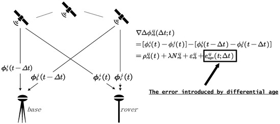
Figure 1. The illustration of the observation error introduced by the differential age in the DD operation.

Considering short baseline cases, ignoring the atmospheric parameter difference introduced by the spatial factor [34], and substituting (1) into (2), the following can be derived:

$$\begin{array}{c}\hfill \nabla \Delta {\varphi }_{rb}^{ij}(\Delta t;t)={\rho }_{rb}^{ij}\left(t\right)+\lambda N_{rb}^{ij}+{\epsilon }_{rb}^{ij}+[-I^{ij}\left(t\right)+T^{ij}\left(t\right)-cd{t}^{ij}\left(t\right)+o^{ij}\left(t\right)]\\ \hfill -[-I^{ij}(t-\Delta t)+T^{ij}(t-\Delta t)-cd{t}^{ij}(t-\Delta t)+o^{ij}(t-\Delta t)]\end{array}$$

(3)

Define

$$\begin{array}{c}\hfill f^i\left(t\right)=[T^i\left(t\right)-I^i\left(t\right)-cd{t}^i\left(t\right)+o^i\left(t\right)],\end{array}$$

(4)

and

$$\begin{array}{cc}\hfill e_{age}^{ij}(t;\Delta t)& =[f^i\left(t\right)-f^j\left(t\right)]-[f^i(t-\Delta t)-f^j(t-\Delta t)]\hfill \\ \hfill & =[f^i\left(t\right)-f^i(t-\Delta t)]-[f^j\left(t\right)-f^j(t-\Delta t)].\hfill \end{array}$$

(5)

Then, the DD observation in (3) can be expressed as follows:

$$\begin{array}{c}\hfill \nabla \Delta {\varphi }_{rb}^{ij}(\Delta t;t)={\rho }_{rb}^{ij}\left(t\right)+\lambda N_{rb}^{ij}+{\epsilon }_{rb}^{ij}+e_{age}^{ij}(t;\Delta t).\end{array}$$

(6)

where ${\epsilon }_{rb}^{ij}$ is the DD observation noise, ${\epsilon }_{rb}$ is the vector form of all the visible satellite observations, and the covariance matrix of ${\epsilon }_{rb}$ is ${\mathsf{\Omega }}_{dd}$, i.e., ${\epsilon }_{rb}\sim N(0,{\mathsf{\Omega }}_{dd})$. In the widely used ARTK [12,13,14,15] DD observation model, only the first three items are considered. Here, we introduce the differential age error item, i.e., $e_{age}^{ij}(t;\Delta t)$, which denotes the DD error at time t caused by the differential age $\Delta t$. The main aim of this study is to improve the RTK application performance by modeling, estimating, and compensating for the differential age error $e_{age}^{ij}(t;\Delta t)$.

2.2. Estimation and Compensation Methods

The overall system block diagram is presented in Figure 2. As illustrated in the figure, the data processing involved in this study is divided into three parts: (1) the conventional asynchronous DD observation calculation (shown in the pink boxes); (2) the differential age error estimation, prediction, and compensation proposed in this paper (shown in the yellow boxes); and (3) the proposed predictor performance monitor for the integrity assessment (shown in the green boxes). We provide a detailed description of each part in the following sections.

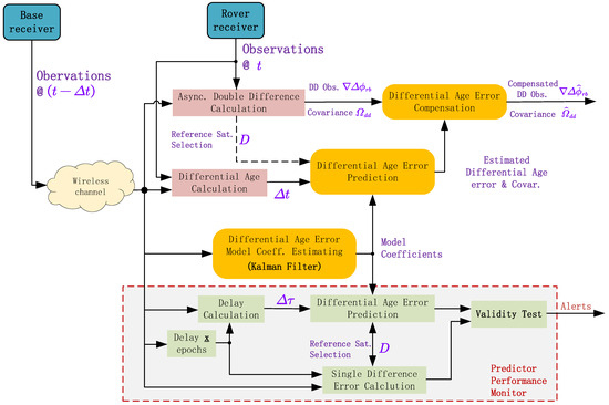
Figure 2. The system diagram of the proposed method.

2.2.1. Modeling and Estimating the Differential Age Error

Notice the elements in (4), i.e., the atmospheric delay, satellite clock error, and orbit error, vary slowly over time. In other words, they each can be represented by a smooth mathematical function. By expanding this at time t using the Taylor series, the following can be obtained:

$$\begin{array}{cc}\hfill f^i(t+\Delta t)& =f^i\left(t\right)+{f^i}^{\prime }\Delta t+{\displaystyle \frac{1}{2}}{f^i}^{″}\Delta t^2+\dots \hfill \\ \hfill & \approx f^i\left(t\right)+{\alpha }^i\left(t\right)\Delta t\hfill \end{array}$$

(7)

where ${(.)}^{\prime }$ and ${(.)}^{″}$ denote the first and second derivative term, respectively. To trade off the model stability and accuracy, only the first term of the Taylor series is retained, and the higher-order terms are ignored. For convenience, defining ${\alpha }^i\left(t\right)$ as the first derivative of $f^i\left(t\right)$ at time t and substituting (7) into (5) gives:

$$e_{age}^{ij}(t;\Delta t)\approx ({\alpha }^i\left(t\right)-{\alpha }^j\left(t\right))\Delta t.$$

(8)

Then, the next task is to estimate the item ${\alpha }^i\left(t\right)-{\alpha }^j\left(t\right)$ from base station observations.

The accurate position of the base station in the Earth-Centered, Earth-Fixed (ECEF) coordinate system is already known. Thus, using the broadcast ephemeris, the observation equation for the satellite carrier phase can be formulated as follows:

$$v_{\varphi }^i\left(t\right)=f^i\left(t\right)+cd{t}_b\left(t\right)+{\delta }_b+\lambda {\varphi }_b+{\delta }^i+\lambda ({\varphi }^i+N^i)+{\epsilon }_b^i$$

(9)

where $v_{\varphi }^i={\varphi }_b^i\left(t\right)-{\rho }_b^i$ is the observed-minus-computed (OMC) term of the undifferentiated carrier phase. The variance in the observation error ${\sigma }_b^i$ (i.e., ${\epsilon }_b^i\sim N(0,{\sigma }_b^i)$) can be calculated using the sine function model of elevation [35,36]:

$${\sigma }_b^i=a^2+{\displaystyle \frac{b^2}{si{n}^{2}El}}$$

(10)

where $El$ is the satellite elevation. For geodetic GNSS receivers, the values of a and b are usually approximately 4.3 mm and 3 mm, respectively.

The time-differenced carrier phase (TDCP) ratio is defined as follows:

$$r_{tdcp}^i={\displaystyle \frac{v_{\varphi }^i\left(t\right)-v_{\varphi }^i(t-\Delta t)}{\Delta t}}$$

(11)

as a new observation. Moreover, combining (9) and (7), we obtain the following:

$$r_{tdcp}^i={\alpha }^i+{\eta }_r+{\tilde{\epsilon }}^i$$

(12)

where

$${\eta }_r={\displaystyle \frac{cd{t}_b\left(t\right)-cd{t}_b(t-\Delta t)}{\Delta t}},$$

(13)

and ${\tilde{\epsilon }}^i$ is the time-differentiated observation noise:

$${\tilde{\epsilon }}^i={\displaystyle \frac{2}{\Delta t}}{\epsilon }_b^i,$$

(14)

with variance ${\tilde{\sigma }}^i$, i.e., ${\tilde{\epsilon }}^i\sim N(0,{\tilde{\sigma }}^i)$, then, ${\tilde{\sigma }}^i={\displaystyle \frac{4}{{\Delta t}^2}}{\sigma }_b^i$. Since the first-order derivative ${\alpha }^i\left(t\right)$ is a value fluctuating around zero, it is reasonable to assume it is a first-order Gauss–Markov process. The receiver clock fluctuation ${\eta }_r\left(t\right)$ is assumed to be a random walk process. In addition, the item ${\eta }_r\left(t\right)$ is eliminated in later processing.

$$\left\{\begin{array}{cc}\dot{{\alpha }^i}\hfill & ={\displaystyle \frac{1}{{\xi }^i}}{\alpha }^i+n_{\alpha }^i\hfill \\ \dot{{\eta }_r}\hfill & =n_{{\eta }_r},\hfill \end{array}\right.$$

(15)

where ${\xi }^i$ and $n_{\alpha }^i$ are the correlated time and process noise for $\alpha$, respectively; $n_{\alpha }^i$ follows a zero-mean normal distribution, i.e., $n_{\alpha }^i\sim N(0,q^i)$; and $n_{{\eta }_r}$ is the process noise of ${\eta }_r$, following a zero-mean normal distribution, i.e., $n_{{\eta }_r}\sim N(0,q_r)$.

From the above model and assumption, we can set up the state transformation and observation function to estimate the differential age error. The state vector is defined as follows:

$$\mathit{x}={[{\alpha }^1{\alpha }^2\dots {\alpha }^L{\eta }_r]}^T.$$

(16)

Using the assumption in (15), we can obtain the following:

$$\dot{\mathit{x}}=\mathit{F}\mathit{x}+{\mathit{n}}_{\mathit{t}},$$

(17)

where

$$\mathit{F}=\left[\begin{array}{cccc}1/{\xi }^1& 0& \dots & 0\\ 0& 1/{\xi }^2& \dots & 0\\ 0& 0& \dots & 0\\ 0& 0& \dots & 1\end{array}\right]$$

(18)

and

$${\mathit{n}}_{\mathit{t}}={[n_{\alpha }^1{n}_{\alpha }^2\dots n_{\alpha }^L{n}_{{\eta }_r}]}^T.$$

(19)

where $\mathit{F}$ and ${\mathit{n}}_{\mathit{t}}$ are the state transform matrix and process noise vector, respectively; ${\mathit{n}}_{\mathit{t}}\sim N(0,\mathit{Q})$, $\mathit{Q}$ is the covariance matrix.

$$\mathit{Q}=\left[\begin{array}{ccccc}{q}^1& 0& \dots & 0& 0\\ 0& q^2& \dots & 0& 0\\ 0& 0& \dots & 0& 0\\ 0& 0& \dots & q^L& 0\\ 0& 0& \dots & 0& q_r\end{array}\right].$$

(20)

By combining all TDCP ratio measurements for each satellite together, the observation vector can be defined as follows:

$$\mathit{z}={[r_{tdcp}^1\left(t\right)r_{tdcp}^2\left(t\right)\dots r_{tdcp}^L\left(t\right)]}^T.$$

(21)

According to (12) and the state vector definition (16), the observation function can be obtained:

$$\mathit{z}=\mathit{H}\mathit{x}+\mathit{ϵ}$$

(22)

where the observation matrix $\mathit{H}$ is as follows:

$$\mathit{H}=\left[\begin{array}{cccc}1& 0& \dots & 1\\ 0& 1& \dots & 1\\ 0& 0& \dots & 1\\ 0& 0& \dots & 1\end{array}\right].$$

(23)

Assuming the observations are independent of each other, the observation noise $\mathit{ϵ}$ is a Gaussian distribution vector with diagonal covariance, i.e., $\mathit{ϵ}\sim N(0,\mathit{R})$ and $\mathit{R}=diag({\tilde{\sigma }}^1{\tilde{\sigma }}^2\dots {\tilde{\sigma }}^L)$.

2.2.2. The Simplified Estimator with Equivalence Transformation and Sequential Kalman Filter

As shown in the previous section, we can already estimate the differential age error parameters directly using the conventional Kalman filter algorithm. However, obviously, the receiver clock fluctuating item ${\eta }_r$ is not related to the estimation and compensation of the differential age error. In this section, a simplified estimating algorithm with superior computing efficiency is described with equivalence transformation and sequential Kalman filter techniques.

Notice that

$$\mathit{H}=\left[{\mathit{B}}_{\mathbf{1}}{\mathit{B}}_{\mathbf{2}}\right]$$

(24)

where ${\mathit{B}}_{\mathbf{1}}=\mathit{I}$, ${\mathit{B}}_{\mathbf{2}}={[11\dots 1]}^T$.

Thus, according to the equivalence transformation principle [30,31], the observation function can be transformed into the following:

$$\begin{array}{cc}\hfill \mathit{z}& =\mathit{M}{\mathit{B}}_{\mathbf{1}}{\mathit{x}}^{\prime }+{\mathit{ϵ}}^{\prime }\hfill \\ \hfill & =\mathit{M}{\mathit{x}}^{\prime }+{\mathit{ϵ}}^{\prime },\hfill \end{array}$$

(25)

where ${\mathit{ϵ}}^{\prime }$ has the same statistic properties as $\mathit{ϵ}$, i.e., ${\mathit{ϵ}}^{\prime }\sim N(0,\mathit{R})$, and

$${\mathit{x}}^{\prime }={[{\alpha }^1{\alpha }^2\dots {\alpha }^L]}^T,$$

(26)

and

$$\mathit{M}=\mathit{I}-{\mathit{B}}_{\mathbf{2}}{\left({\mathit{B}}_{\mathbf{2}}^T\mathit{R}{\mathit{B}}_{\mathbf{2}}\right)}^{-1}{\mathit{B}}_{\mathbf{2}}^T\mathit{R}.$$

(27)

In this case, ${\mathit{B}}_{\mathbf{2}}$ and $\mathit{R}$ have special structures: ${\mathit{B}}_{\mathbf{2}}$ is an all-one vector, and $\mathit{R}$ is a diagonal matrix. Hence, $\mathit{M}$ can be simplified as follows:

$$\mathit{M}=-{\left(\sum _{\mathit{i}}{\tilde{\sigma }}^i\right)}^{-1}\left[\begin{array}{cccc}{\tilde{\sigma }}^1-\sum _{\mathit{i}}{\tilde{\sigma }}^i& {\tilde{\sigma }}^2& \dots & {\tilde{\sigma }}^L\\ {\tilde{\sigma }}^1& {\tilde{\sigma }}^2-\sum _{\mathit{i}}{\tilde{\sigma }}^i& \dots & {\tilde{\sigma }}^L\\ {\tilde{\sigma }}^1& {\tilde{\sigma }}^2& \dots & {\tilde{\sigma }}^L\\ {\tilde{\sigma }}^1& {\tilde{\sigma }}^2& \dots & {\tilde{\sigma }}^L-\sum _{\mathit{i}}{\tilde{\sigma }}^i\end{array}\right..$$

(28)

Hence, we can obtain the Kalman filter expression:

$$\begin{array}{c}\hfill \left\{\begin{array}{cc}{\mathit{x}}^{-}\hfill & =\mathit{A}{\mathit{x}}^{\prime }\hfill \\ {\mathit{P}}^{-}\hfill & =\mathit{A}\mathit{P}{\mathit{A}}^T+\mathit{Q}\hfill \end{array}\right.\end{array}$$

(29)

and prediction step:

$$\begin{array}{c}\hfill \left\{\begin{array}{cc}\mathit{K}\hfill & ={\mathit{P}}^{-}{\mathit{M}}^T{(\mathit{M}{\mathit{P}}^{-}{\mathit{M}}^T+\mathit{R})}^{-1}\hfill \\ {\mathit{x}}^{\prime }\hfill & ={\mathit{x}}^{-}+\mathit{K}(\mathit{z}-\mathit{M}{\mathit{x}}^{-})\hfill \\ \mathit{P}\hfill & =(\mathit{I}-\mathit{K}\mathit{M}){\mathit{P}}^{-},\hfill \end{array}\right.\end{array}$$

(30)

where

$$\begin{array}{cc}\hfill \mathit{A}=exp(\mathit{F}\Delta t)& \hfill \approx \mathit{I}+\Delta t\mathit{F}\end{array}$$

(31)

Since it is reasonable to assume the observations are independent, the sequential Kalman filtering technique is used here to avoid the computationally complex matrix inversion operation. Hence, the updating step for the estimator, which works sequentially for $i\in [1,2,\dots ,L]$, can be implemented as follows:

$$\begin{array}{c}\hfill \left\{\begin{array}{c}{\mathit{K}}_i\leftarrow \mathit{P}{\mathit{M}}_{\mathit{i}}^T{({\mathit{M}}_{\mathit{i}}\mathit{P}{\mathit{M}}_{\mathit{i}}^T+R_{ii})}^{-1}\hfill \\ {\mathit{x}}^{\prime }\leftarrow {\mathit{x}}^{\prime }+{\mathit{K}}_i(z_i-{\mathit{M}}_i{\mathit{x}}^{\prime })\hfill \\ \mathit{P}\leftarrow (\mathit{I}-{\mathit{K}}_i{\mathit{M}}_i)\mathit{P},\hfill \end{array}\right.\end{array}$$

(32)

where the initial values of ${\mathit{x}}^{\prime }$ and $\mathit{P}$ are ${\mathit{x}}^{-}$ and ${\mathit{P}}^{-}$, respectively; ${\mathit{K}}_i$ is the ith column of matrix $\mathit{K}$; and ${\mathit{M}}_i$ is the ith row of matrix $\mathit{M}$.

According to the analysis in [37], the computational complexities of the standard Kalman filter and sequential filter are approximately $[2{\overline{D}}^2\overline{S}+\overline{k}{\overline{D}}^3+2\overline{D}\ast {\overline{S}}^2]$ and $[2\overline{D}\ast {\overline{S}}^2]$, respectively, where $\overline{D}$ and $\overline{S}$ are the dimensions of the observation vector and state vector, respectively, and $\overline{k}$ is a scalar associated with matrix inversion calculation. Consider that the number of observations and the dimension of the state vector are the same, which is the number of satellites L. The computational complexity of the simplified estimator is $\left[2L^3\right]$, while, in contrast, the computational complexity of the standard Kalman filter is $[(\overline{k}+4)L^3+6L^2+2L]$.

2.2.3. Compensating for the Differential Age Error in the DD Operation

When ${\alpha }^i$ for each observed satellite is estimated, the differential age error for the DD operation can be obtained.

The differential matrix D for the differential operation between norm satellites and reference satellites can be defined as follows:

$$\begin{array}{c}\hfill D=\left[\begin{array}{cccccc}1& 0& \cdots & -1& \cdots & 0\\ 0& 1& \cdots & -1& \cdots & 0\\ ⋮& ⋮& \ddots & ⋮& \ddots & ⋮\\ 0& 0& \cdots & \underbrace{-1}& \cdots & 0\\ & & & jth& & \end{array}\right]\end{array}$$

(33)

Then, the estimated differential age error is

$$\begin{array}{c}\hfill {\widehat{\mathit{e}}}_{\mathit{age}}(t;\Delta t)={\mathit{Dx}}^{\prime }\Delta t.\end{array}$$

(34)

where D and $x^{\prime }$ are the differential matrix and estimated $\alpha$ in the current epoch t, and ${\widehat{\mathit{e}}}_{\mathit{age}}$ is the vector form of ${\widehat{e}}_{age}^{ij}$.

The final covariance of the DD observation with prediction error uncertainty is as follows:

$$\begin{array}{c}\hfill {\widehat{\mathsf{\Omega }}}_{dd}={\mathit{DPD}}^T{(\Delta t)}^2+{\mathsf{\Omega }}_{dd}\end{array}$$

(35)

where $\mathit{P}$ is the predicting covariance matrix in the current epoch, and ${\mathsf{\Omega }}_{dd}$ is the original DD observation covariance matrix.

2.2.4. Predictor Performance Monitor

The performance of the aforementioned error predictor is highly dependent on how well the established model aligns with actual physical behaviors. However, it is challenging to ensure complete consistency between the model and real physical behavior. If the model’s predictions significantly deviate from the true values while providing a small variance, it could lead to errors in subsequent integrity assessments, resulting in systematic risks.

To address this, a predictor performance monitor was designed to assess the predictor’s performance. When significant deviations in prediction performance are detected (e.g., during abnormally active ionospheric conditions), the system provides warning information for subsequent processing, which enhances the overall system integrity. The performance monitor functions by using historical base station observation data and subsequent base station observation data to calculate the actual age errors. It then performs a chi-square test with the predicted age errors. If the actual errors and predicted errors are statistically consistent, the performance meets the requirements. If they are statistically inconsistent, it indicates that the current prediction model and parameters are at risk.

The real base station age error can be calculated by the following operations:

$$\begin{array}{c}\hfill e_{\Delta \tau }^{ij}=[v_{\varphi }^i\left(t_0\right)-v_{\varphi }^i\left(t_1\right)]-[v_{\varphi }^j\left(t_0\right)-v_{\varphi }^j\left(t_1\right)],\end{array}$$

(36)

and

$$\begin{array}{c}\hfill \Delta \tau =t_0-t_1,\end{array}$$

(37)

where $v_{\varphi }^i\left(t_0\right)$ is the base station’s OMC of satellite i as defined in (9) at epoch $t_0$, and $v_{\varphi }^i\left(t_1\right)$ is the OMC for the previous epoch $t_1$; $v_{\varphi }^j\left(t_0\right)$ and $v_{\varphi }^j\left(t_1\right)$ are the OMCs of the reference satellite j at epoch $t_0$ and epoch $t_1$, respectively. For convenience, the vector form of the error can be defined as follows:

$$\begin{array}{c}\hfill {\mathit{e}}_{\Delta \tau }=\mathit{D}[{\mathit{v}}_{\varphi }\left(t_0\right)-{\mathit{v}}_{\varphi }\left(t_1\right)],\end{array}$$

(38)

where ${\mathit{e}}_{\Delta \tau }$ and ${\mathit{v}}_{\varphi }$ are the vector forms of $e_{\Delta \tau }^{ij}$ and $v_{\varphi }^i\left(t_0\right)$, respectively, and $\mathit{D}$ is defined as (33).

In addition, the prediction and the covariance can be calculated as (34) and (35):

$$\begin{array}{c}\hfill {\widehat{\mathit{e}}}_{\Delta \tau }={\mathit{Dx}}^{\prime }\Delta \tau \end{array}$$

(39)

and

$$\begin{array}{c}\hfill {\widehat{\mathsf{\Omega }}}_{\Delta \tau }={\mathit{DPD}}^T{(\Delta \tau )}^2,\end{array}$$

(40)

where ${\widehat{\mathit{e}}}_{\Delta \tau }$ and ${\widehat{\mathsf{\Omega }}}_{\Delta \tau }$ are the prediction age error and its covariance, respectively.

The following statistic is constructed to test whether the model is valid:

$$\begin{array}{c}\hfill \mathsf{\Gamma }={[{\widehat{\mathit{e}}}_{\Delta \tau }-{\mathit{e}}_{\Delta \tau }]}^T{{\widehat{\mathsf{\Omega }}}_{\Delta \tau }}^{-1}[{\widehat{\mathit{e}}}_{\Delta \tau }-{\mathit{e}}_{\Delta \tau }],\end{array}$$

(41)

where L is the number of satellites observed, and $\mathsf{\Gamma }$ should follow a chi-square distribution with freedom $L-1$, i.e, $\mathsf{\Gamma }\sim {\chi }^2(L-1)$.

Then, the validity of the model can be evaluated by comparing the statistic and chi-square value:

$$\begin{array}{c}\hfill \left\{\begin{array}{c}\mathbf{Valid}:\mathsf{\Gamma }<{\chi }^2(L-1,0.05);\hfill \\ \mathbf{Risk}:\mathsf{\Gamma }\ge {\chi }^2(L-1,0.05).\hfill \end{array}\right.\end{array}$$

(42)

where the risk level set to $5\%$. Notice that the model performance is related to the prediction age, i.e., $\Delta \tau$ or $\Delta t$. A batch of epoch intervals ($\Delta \tau$) can be chosen to evaluate the prediction performance with various differential ages.

3. Experiments and Results

Static and kinematic experiments were conducted to demonstrate the effectiveness of the proposed method.

In the static experiment, the accuracy of differential-age compensation was evaluated using a 24 h dataset, in which both BDS and GPS techniques were analyzed. In the kinematic experiment, the proposed method was incorporated into RTK processing. Subsequently, a statistical analysis and comparison were conducted for the proposed method and the ARTK prediction method in terms of the fixed rate and false rate of integer ambiguities, etc. The observations were collected during the experiments and then post-processed.

3.1. Static Experiment and Results

A 24 h static experiment was carried out, and a 1 Hz observation was conducted using a Mosaic-x5 GNSS receiver board (from Septentrio N.V.) through an antenna mounted on the building’s roof. The static experiment information is shown in Table 2.

Table 2. Static experiment information.

Navigation Satellite Systems	GNSS Receiver	Carrier Frequency	Data Rate	Start Epoch (TOW)	End Epoch (TOW)	Total Epochs
GPS/BDS	Mosaic-x5	L1/B1I	1 Hz	281,453.0 s	368,632.0 s	87,179 s

During the 24 h static experiment, the GNSS antenna’s view was clear, and there was no signal blockage around the antenna. In the subsequent data processing, the cutoff elevation angle was set to 15 degrees. The carrier-to-noise ratio densities (C/N0) of all visible satellites, including GPS and BDS satellites, were all over 35 dBHz, the observation data were continuous, and the number of BDS satellites was greater than that of GPS satellites.

Figure 3 gives the undifferentiated carrier phase observation minus calculation (OMC) during the experiment, i.e., the expression $v_{\varphi }^i$ in (9). Each line in the figure presents one satellite observation. Notice that because the receiver’s position was known accurately as a prior, the curve ripples in Figure 3 were mainly caused by satellite orbit/clock and atmospheric compensation errors. Variations in the receiver’s clock error also contributed to the curve ripples; however, this can be eliminated by the differential operation between satellites.

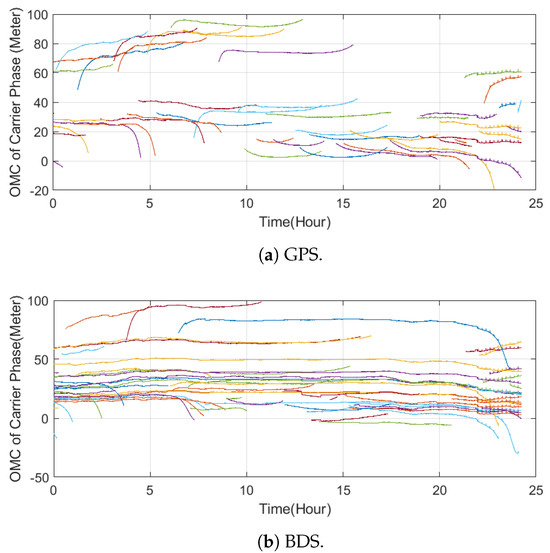
Figure 3. The undifferentiated carrier phase observation minus calculation (OMC) during the experiment. Note: Each curve represents one satellite’s carrier phase.

The proposed prediction method and the ARTK prediction method were compared for various differential ages (up to 120 s). Predictions based on historical data were compared with subsequently received data, which served as the reference ground truth. Each valid epoch was evaluated with both methods across different differential ages. To eliminate the items caused by the receiver, the single difference (SD) between satellites’ prediction residuals was calculated by selecting reference satellites in each satellite system. The ground truth of the predicted value was calculated by the data received in that epoch. Then, the root mean square error (RMSE) of single-difference prediction residuals between satellites was calculated at each second within differential ages. The single difference between the satellite prediction residuals’ RMSE calculation method is as follows:

$$\begin{array}{c}\hfill RMS{E}^i\left({\tau }_{age}\right)=\sqrt{{\displaystyle \frac{{\sum }_{k=1}^N{\left[\left(v_{\varphi }^i\left(t_k\right)-v_{\varphi }^{ref}\left(t_k\right)\right)-\left(y^i(t_k;{\tau }_{age})-y^{ref}(t_k;{\tau }_{age})\right)\right]}^2}{N}}},\end{array}$$

(43)

where $RMS{E}^i\left({\tau }_{age}\right)$ is the prediction root mean square error of the satellite i with the differential age ${\tau }_{age}$; N is the total prediction sets; $t_k$ is the time at kth epoch; $y^i(t_k;{\tau }_{age})$ and $y^{ref}(t_k;{\tau }_{age})$ denote the prediction residuals (OMC) of the satellite i and the reference satellite $ref$ with differential age ${\tau }_{age}$ at epoch k, respectively; $v_{\varphi }^i\left(t_k\right)$ and $v_{\varphi }^{ref}\left(t_k\right)$ represent the actual or non-predicted OMC of the satellite i and reference satellite $ref$ at epoch k, respectively. Notice that the reference satellite changed during the experiment but remained the same for the ground truth and prediction. For the ARTK method, the prediction item $y^i(t_k;{\tau }_{age})$ was simply taken as a history value, i.e., $y^i(t_k;{\tau }_{age})=v_{\varphi }^i(t_k-{\tau }_{age})$.

Figure 4 shows the time domain comparison between the actual observations received, the predicted values of the method proposed in this work, and the ARTk method’s predicted values. Due to space limitations, only the case featuring the 120 s differential age and BDS satellite observation is shown here. To eliminate the local receiver’s clock error fluctuation, the curves shown in the figure are single-difference carrier phase observations with the reference satellite. Each curve represents a single-difference carrier observation. It is shown that the changes in SD observations over time were generally smooth, and some observations exhibited significant changes over time. The ARTK method only shifts historical observations, so it generates large errors when the observations change significantly over time. The method proposed in this article can better track the changes over time and can achieve a substantial improvement in prediction performance. It is worth noting that because the prediction method used in this work is independent of reference satellite selection, it can be easily managed when the reference satellites change.

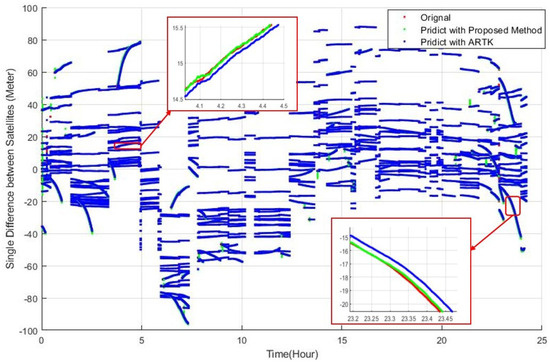
Figure 4. The predicted single-difference observation with the proposed method and ARTK method. Note: Each curve represents one satellite’s carrier phase.

Figure 5 shows the RMSE of each satellite under different differential ages using the ARTK and the proposed method. The specific RMSE calculation method is described in Equation (43). The BDS and GPS results are presented in the sub-figures. The observations were compensated using broadcast ephemeris data, including atmospheric, satellite orbit, and clock errors. As shown in Figure 5a,c, when the ARTK method was adopted, the RMSE prediction was within 10 cm at a 20 s differential age, for both the GPS and BDS. For such a prediction error, the RTK algorithm can usually obtain a fixed solution. However, as the differential age increased, eventually reaching more than 60 s, nearly half of the GPS’s RMSE predictions were greater than 10 cm, and a large part of the carrier’s RMSE predictions using the BDS were also greater than 10 cm. Under such a differential age, even if the partial ambiguity fixed RTK algorithm is adopted, the probability of obtaining a fixed solution is significantly reduced. When the differential age was 120 s, most carrier RMSEs were greater than 10 cm, with the maximum being 60 cm. Thus, it can be assumed that the RTK algorithm will find it challenging to obtain a fixed solution in this case.

Figure 5. The RMSE comparison of the prediction residual with two methods, with reference to the differential age, for the GPS and BDS. Note: Each curve represents one satellite’s carrier phase.

For comparison, Figure 5b,d present the RMSE of the proposed prediction method with reference to different differential ages. It can be seen that the RMSE significantly decreased with the proposed prediction method as the differential age increased. At a differential age of 60 s, the RMSE of the GPS’s measurements was less than 8 cm, and the RMSE of the BDS measurements was less than 4 cm. For the RTK algorithm, the probability of obtaining a fixed solution is very high in this case. When the differential aging period increased to 120 s, the RMSE of most carriers in the GPS was also less than 10 cm, and the RMSE of all carriers in the BDS was less than 8 cm. The probability of obtaining a fixed solution using a partial ambiguity fixed RTK algorithm is very high in this case.

Figure 6 presents a comparison of the overall RMSE for the proposed and ARTK method. The definition of the overall RMSE is as follows:

$$\begin{array}{c}\hfill RMS{E}_{overall}\left({\tau }_{age}\right)=\sqrt{{\displaystyle \frac{{\sum }_{i=1}^{M}RMS{E}^i{\left({\tau }_{age}\right)}^2}{M}}},\end{array}$$

(44)

where M is the total observed carrier number.

Figure 6. The overall RMSE comparison for the proposed method and ARTK method with reference to the differential age.

In Figure 6, it is clear that the proposed method exhibited a significant improvement in prediction performance as compared to the ARTK method. At a differential age of 60 s, the overall RMSE of the GPS reduced from 16 cm to 5.7 cm, and the overall RMSE of the BDS reduced from 11 cm to 2 cm. At a differential age of 120 s, the overall RMSE decreased from 28.9 cm to 8.7 cm for the GPS and from 19 cm to 3.5 cm for the BDS. Therefore, it can be expected that, for the RTK algorithm, the proposed method will generate a significant increase in the fixed rate for large differential age scenarios.

3.2. Kinematics Experiments and Results

To further investigate the effectiveness of the proposed method in RTK applications, a field test with a land vehicle was carried out in Chengdu, China, on 27 December 2023.

The vehicle platform utilized in the test was the model EX5 SUV from Weltmeister Motor Co., Ltd., (Shanghai, China) and the rover station’s GNSS antenna was installed on the vehicle’s roof. The rover GNSS receiver was an LG69T from Quectel Co., Ltd. (Shanghai, China). Its supported frequency band includes L1 C/A and L5 for GPS/QZSS, E1 and E5a for Galileo, and B1I and B2a for BDS. Its observed data output frequency was set to 5 Hz. The Novatel’s SPAN-ISA-100C integrated navigation system was adopted as the reference ground truth system. This includes two GNSS receivers, PwrPak7D, and a high-precision inertial measurement unit (IMU): IMU-ISA-100C. One PwrPak7D receiver was used as the base station receiver, and the base station antenna was installed on the building’s roof at a known coordinate. Another PwrPak7D receiver and IMU-ISA-100C were installed in the trunk of the car as rover stations. The radio frequency signal from the GNSS antenna on the EX5 vehicle’s roof was split two ways, i.e., the LG69T and PwrPak7D receivers. The LG69T observation data were saved in the portable computer through a USB port, and the SPAN-ISA-100C observation data were saved in PwrPak7D. The observation data saved by PwrPak7D were post-processed using the post-processing software from Novatel (Calgary, Canada), i.e., Inertial Explorer (Version 8.90).

The field experiment setup is shown in Figure 7, the kinematic experiment information is shown in Table 3, and the whole field test trajectory obtained by IE is shown in Figure 8.

Figure 7. The experimental setup.

Table 3. Field experiment information.

Navigation Satellite Systems	Carrier Frequency	Rover Receiver	Base Receiver	Reference System
GPS/BDS	L1/B1I	Quectel LG69T (5 Hz)	Novatel PwrPak7D (1 Hz)	Novatel SPAN-ISA-100C

Figure 8. The trajectory of the field experiment.

As shown in Figure 8, the field kinematic experiment scene included various scenarios, e.g., boulevards, urban canyons, overpasses, and open-sky. Figure 9 shows the sky plot and the number of satellites observed during the experiment. The figure shows that more than 20 GPS/BDS satellites were observed during most of the experiment.

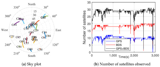
Figure 9. The sky plot and number of satellites observed in the field experiment.

The open-source software Rtklib was utilized for post-processing the RTK calculations. In the original version of Rtklib, the asynchronous RTK (ARTK) method was adopted to handle large differential ages. The proposed prediction method was integrated into the original version as a modified version of Rtklib. A comparison between the original and modified versions was conducted to evaluate the effectiveness of the proposed method.

The RTK solution without differential aging, i.e., synchronous RTK, was also included in the comparison to obtain the baseline performance. Since the base station and rover’s observation data rates were 1 Hz and 5 Hz, respectively, it was impossible to completely align the base and rover data. Therefore, rover observations at non-integer seconds were calculated with the nearest integer-second base station observation data. That is to say that when the differential aging was less than 1 s, it was considered a synchronous RTK solution.

In the simulation, various differential ages of 40 s, 60 s, 80 s, 100 s, and 120 s were introduced, and RTK solutions were calculated using the ARTK and the proposed method. For example, Figure 10 presents the fixed states over time using the two algorithms with a differential age of 120 s. The fixed rates and false fixed rates of the integer ambiguity for the two methods were statistically calculated for each differential age. Here, the false fixed solution denotes an incorrect fixed solution. The specific method of determination was to compare the RTK positioning results with the reference value. When the RTK calculated result was a fixed solution and the absolute positioning error was greater than 0.1 m, the fixed solution of the epoch was considered to be a false fixed solution.

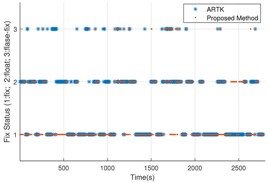
Figure 10. The fixed status (in time) comparison of the two methods with a 120 s differential age.

Table 4 presents the fixed and false fixed rates of the proposed and ARTK methods under various differential aging periods. It can be seen that, as the differential age increases, the ambiguity fixed rate gradually decreases. However, the fixed rate with the proposed prediction method is always higher than that of the ARTK method. Specifically, as shown in the table, the synchronous RTK method exhibited the highest integer ambiguity fixed rate and the lowest false fixed rate. When the differential age was 40 s, the ambiguity fixed rate of both methods was similar. When the difference age was 60 s, the ambiguity fixed rate and false fixed rate of the ARTK method were 0.90 times and 1.63 times that of the proposed method, respectively. In addition, when the difference age was 120 s, the values were 0.78 times and 4.78 times that of the proposed method, respectively, resulting from the rapid increase in the observation prediction error of the ARTK method with the increase in the base station differential age.

Table 4. The statistical results of the integer ambiguity with various differential ages.

RTK Methods	Total Epochs (s)	Differential Age (s)	Fixed Epochs	Fixed Rate	False Fixed Epochs	False Fixed Rate
Synchronized RTK	13,666	<1	13,567	97.7%	114	0.8%
The Proposed method	13,666	40	12,401	90.7%	203	1.6%
		60	12,002	87.8%	231	1.9%
		80	11,564	84.6%	163	1.4%
		100	11,311	82.8%	171	1.5%
		120	9752	71.4%	180	1.8%
The ARTK method	13,666	40	12,263	89.7%	434	3.5%
		60	10,817	79.2%	338	3.1%
		80	9187	67.2%	557	6.1%
		100	8098	59.3%	449	5.5%
		120	7613	55.7%	652	8.6%

In conclusion, in the field test, the proposed prediction method significantly improved the fixed rate of the RTK algorithm and significantly reduced the false fixed rate compared with the traditional ARTK method in the case of a large differential age.

4. Discussion

Differential age errors are mainly caused by fluctuations in the satellite clock, orbit prediction errors, and atmospheric errors. The proposed method utilizes the fact that these errors vary slowly and relatively smoothly and then models them with a truncated Taylor series. Furthermore, equivalent transformation and sequential filtering technology were adopted to enhance the computational efficiency. In the proposed method, the errors caused by several sources are lumped together, making it more straightforward and less dependent on prior information than the SSR methods.

Nonetheless, as is well known, the effectiveness of the Kalman estimator largely depends on whether the established/assumed model matches the real physical world. Although the proposed model can generally achieve satisfactory results, which is demonstrated by the experimental data, this model may not always perfectly match real-world physical behaviors. According to analyses in several studies [15,16,20,21,22,23], ionospheric errors are the most challenging factor to predict over time. In [38], the temporal correlation of the ionospheric error is investigated in detail based on 11 years of observational data from different geographic regions. It is demonstrated that the temporal correlation of the ionospheric error is significantly related to the local time, season, solar activity, and geographic latitude, and although statistical values are given, it is not universally effective. In other words, all of the factors above can cause mismatches in the proposed model, resulting in unexpected errors. On this basis, we designed a “Predictor Performance Monitor” to assess the degree of mismatch between the prediction model and actual behavior. When there is a significant discrepancy between the predicted and actual errors, an alert is issued to minimize the system integrity risk as much as possible. From another perspective, a sensitivity analysis is often crucial for understanding an estimation–compensation system. In this model, it is easy to see that, as the prediction differential age increases, the predictor’s prediction error exhibits a linear relationship with it (34). Additionally, other factors related to prediction error, such as model parameters (i.e., Gaussian–Markov process parameters $\{{\xi }^i,q^i\}$ and observation noise variance ${\tilde{\sigma }}^i$), ionospheric activity, and orbital error characteristics, also significantly affect the prediction accuracy. However, the quantitative impact of these factors on prediction performance is difficult to assess, as there can be many modes of mismatch between the proposed model and the actual physical behavior. The combination of various factors makes this analysis a very high-dimensional problem, which in turn, impedes any quantitative analyses. From this perspective, to reduce the systematic risk associated with the proposed approach, it is necessary to simultaneously apply the proposed “Predictor Performance Monitor”.

The accurate adaptive acquisition of random model parameters not only aids in obtaining higher-precision differential age error compensation values but is also crucial for acquiring the precise covariance of double-differenced (DD) observations (${\widehat{\mathsf{\Omega }}}_{dd}$), which significantly impact the RTK ambiguity resolution. Furthermore, practical GNSS observations frequently exhibit outliers for various reasons. To enhance the robustness of the predictor, the proposed method can conveniently incorporate commonly used anomaly detection methods based on the Kalman framework, such as the innovation test and exclusion.

5. Conclusions

In many RTK applications, there is an inevitable time delay between the base station’s and the rover station’s observations. This leads to a rapid increase in the RTK positioning error or fixing failure. In this work, we proposed a differential age error estimation and compensation algorithm based on the Kalman filter to improve performance in these cases. Starting from the carrier phase observation equation, the differential age error model was analyzed and modeled. The estimator of this model was then constructed based on the Kalman filter. Furthermore, equivalent transformation and sequential filtering technology were adopted to significantly reduce the estimator’s computational complexity. Furthermore, a predictor performance monitor was proposed. When the proposed model is inconsistent with real-world physical behavior, an alarm is issued, reducing the system integrity risk.

The statistical results of the 24 h static experiment in Figure 6 and the kinematic experiment statistical results in Table 4 indicate the following:

(1)

The statistical results of the static experiment showed that, when the differential age was 60 s, the GPS and BDS satellites’ overall RMSE according to the ARTK prediction method was 2.8 times and 5.5 times that of the proposed method, respectively. Moreover, when the differential age was 120 s, these values were 3.3 times and 5.4 times that of the proposed method, respectively. This indicates that the accuracy of the base station prediction residuals using the proposed method was much higher than that of the ARTK prediction method.

(2)

The statistical results of the kinematic field experiment showed that, when the differential age was 60 s, the integer ambiguity fixed rate and false fixed rate of the ARTK method were 0.90 times and 1.63 times that of the proposed method, respectively. In addition, at a 120 s differential age, these values were 0.78 times and 4.78 times that of the proposed method, respectively. The proposed method’s integer ambiguity fixed rate and false fixed rate were much better than those of the ARTK method.

In summary, in the case of a large base station differential age, the proposed method can significantly improve the DD observation accuracy, the reliability of RTK integer ambiguity, and the continuity of RTK position solutions. As a result, it effectively meets the requirements for high-precision positioning and continuity in practical applications such as autonomous driving and precision agriculture.

References

- Pirti, A. Performance analysis of the real time kinematic GPS (RTK GPS) technique in a highway project (stake-out). Surv. Rev. 2007, 39, 43–53. [Google Scholar] [CrossRef]
- Odolinski, R.; Odijk, D.; Teunissen, P.J.G. Combined GPS and BeiDou Instantaneous RTK Positioning. Navigation 2014, 61, 135–148. [Google Scholar] [CrossRef]
- Teunissen, P.J.G.; Odolinski, R.; Odijk, D. Instantaneous BeiDou plus GPS RTK positioning with high cut-off elevation angles. J. Geod. 2014, 88, 335–350. [Google Scholar] [CrossRef]
- Wen, W.; Bai, X.; Hsu, L.T. 3D Vision Aided GNSS Real-Time Kinematic Positioning for Autonomous Systems in Urban Canyons. Navigation 2023, 70, navi.590. [Google Scholar] [CrossRef]
- Famiglietti, N.A.; Cecere, G.; Grasso, C.; Memmolo, A.; Vicari, A. A Test on the Potential of a Low Cost Unmanned Aerial Vehicle RTK/PPK Solution for Precision Positioning. Sensors 2021, 21, 3882. [Google Scholar] [CrossRef]
- Pini, M.; Marucco, G.; Falco, G.; Nicola, M.; De Wilde, W. Experimental Testbed and Methodology for the Assessment of RTK GNSS Receivers Used in Precision Agriculture. IEEE Access 2020, 8, 14690–14703. [Google Scholar] [CrossRef]
- Heidari, F.; Fotouhi, R. A Human-Inspired Method for Point-to-Point and Path-Following Navigation of Mobile Robots. J. Mech. Robot. 2015, 7, 041025. [Google Scholar] [CrossRef]
- El-Mowafy, A. Precise real-time positioning using Network RTK. Glob. Navig. Satell. Syst. Signal, Theory Appl. 2012, 7, 161–188. [Google Scholar]
- Feng, Y.; Wang, J. GPS RTK Performance Characteristics and Analysis. J. Glob. Position. Syst. 2008, 7, 1–8. [Google Scholar] [CrossRef]
- El-Mowafy, A. Improving the Performance of RTK-GPS Reference Networks for Positioning in the Airborne Mode. Navigation 2008, 55, 215–223. [Google Scholar] [CrossRef]
- Weber, G.; Dettmering, D.; Gebhard, H. Networked Transport of RTCM via Internet Protocol (NTRIP). In A Window on the Future of Geodesy, Proceedings of the International Association of Geodesy, Sapporo, Japan, 30 June–11 July 2003; Sanso, F., Ed.; Springer: Berlin/Heidelberg, Germany, 2005; Volume 128, pp. 60–64. [Google Scholar]
- Takasu, T.; Yasuda, A. Development of the low-cost RTK-GPS receiver with an open source program package RTKLIB. In Proceedings of the International Symposium on GPS/GNSS, International Convention Center Jeju Korea, Seogwipo-si, Republic of Korea, 4–6 November 2009; Volume 1, pp. 1–6. [Google Scholar]
- Gao, Y.; Liu, Z.; Liu, Z. Internet-based real-time kinematic positioning. GPS Solut. 2002, 5, 61–69. [Google Scholar] [CrossRef]
- Odijk, D.; Wanninger, L. Differential positioning. In Springer Handbook of Global Navigation Satellite Systems; Springer International Publishing: Cham, Switzerland, 2017; pp. 753–780. [Google Scholar]
- Liang, Z.; Hanfeng, L.; Dingjie, W.; Yanqing, H.; Jie, W. Asynchronous RTK precise DGNSS positioning method for deriving a low-latency high-rate output. J. Geod. 2015, 89, 641–653. [Google Scholar] [CrossRef]
- Shu, B.; Liu, H.; Feng, Y.; Xu, L.; Qian, C.; Yang, Z. Analysis of Factors Affecting Asynchronous RTK Positioning with GNSS Signals. Remote Sens. 2019, 11, 1256. [Google Scholar] [CrossRef]
- Lawrence, D.G. Reference Carrier Phase Prediction for Kinematic GPS. U.S. Patent 5,903,236, 5 June 1999. [Google Scholar]
- Du, Y.; Huang, G.; Zhang, Q.; Gao, Y.; Gao, Y. A New Asynchronous RTK Method to Mitigate Base Station Observation Outages. Sensors 2019, 19, 3376. [Google Scholar] [CrossRef]
- Du, Y.; Huang, G.; Zhang, Q.; Tu, R.; Han, J.; Yan, X.; Wang, X. A novel predictive algorithm for double difference observations of obstructed BeiDou geostationary earth orbit (GEO) satellites. Adv. Space Res. 2019, 63, 1554–1565. [Google Scholar] [CrossRef]
- Kashani, I.; Wielgosz, P.; Grejner-Brzezinska, D. The impact of the ionospheric correction latency on long-baseline instantaneous kinematic GPS positioning. Surv. Rev. 2007, 39, 238–251. [Google Scholar] [CrossRef]
- Chen, D.; Ye, S.; Xu, C.; Jiang, W.; Jiang, P.; Chen, H. Undifferenced zenith tropospheric modeling and its application in fast ambiguity recovery for long-range network RTK reference stations. GPS Solut. 2019, 23, 26. [Google Scholar] [CrossRef]
- El-Mowafy, A. On-the-fly prediction of orbit corrections for RTK positioning. J. Navig. 2006, 59, 321–334. [Google Scholar] [CrossRef][Green Version]
- El-Mowafy, A. Impact of predicting real-time clock corrections during their outages on precise point positioning. Surv. Rev. 2019, 51, 183–192. [Google Scholar] [CrossRef]
- Teunissen, P.J.G.; Khodabandeh, A. Review and principles of PPP-RTK methods. J. Geod. 2015, 89, 217–240. [Google Scholar] [CrossRef]
- An, X.; Ziebold, R.; Lass, C. PPP-RTK with rapid convergence based on SSR corrections and its application in transportation. Remote Sens. 2023, 15, 4770. [Google Scholar] [CrossRef]
- Lyu, Z.; Gao, Y. PPP-RTK with augmentation from a single reference station. J. Geod. 2022, 96, 40. [Google Scholar] [CrossRef]
- Khodabandeh, A. Single-station PPP-RTK: Correction latency and ambiguity resolution performance. J. Geod. 2021, 95, 42. [Google Scholar] [CrossRef]
- Khodabandeh, A.; Teunissen, P. An analytical study of PPP-RTK corrections: Precision, correlation and user-impact. J. Geod. 2015, 89, 1109–1132. [Google Scholar] [CrossRef]
- Wang, K.; Khodabandeh, A.; Teunissen, P. A study on predicting network corrections in PPP-RTK processing. Adv. Space Res. 2017, 60, 1463–1477. [Google Scholar] [CrossRef]
- Shen, Y.; Xu, G. Simplified equivalent representation of GPS observation equations. GPS Solut. 2008, 12, 99–108. [Google Scholar] [CrossRef]
- Xu, G. GPS data processing with equivalent observation equations. GPS Solut. 2002, 6, 28–33. [Google Scholar] [CrossRef]
- Teunissen, P.J.G.; Kleusberg, A. GPS for Geodesy; Springer: Berlin/Heidelberg, Germany, 2012; ISBN 978-3-642-72011-6. [Google Scholar]
- Teunissen, P.J.G. The least-squares ambiguity decorrelation adjustment: A method for fast GPS integer ambiguity estimation. J. Geod. 1995, 70, 65–82. [Google Scholar] [CrossRef]
- Teunissen, P.J.G. A canonical theory for short GPS baselines. Part 1: The baseline precision. J. Geod. 1997, 71, 320–336. [Google Scholar] [CrossRef]
- Jin, S.; Wang, J.; Park, P. An improvement of GPS height estimations: Stochastic modeling. Earth Planets Space 2005, 57, 253–259. [Google Scholar] [CrossRef]
- King, R.; Bock, Y. Documentation for the GAMIT GPS Analysis Software, Release 10.2; Scripps Institution of Oceanography: La Jolla, CA, USA, 2009. [Google Scholar]
- Kettner, A.M.; Paolone, M. Sequential discrete Kalman filter for real-time state estimation in power distribution systems: Theory and implementation. IEEE Trans. Instrum. Meas. 2017, 66, 2358–2370. [Google Scholar] [CrossRef]
- Sadegh Nojehdeh, P.; Khodabandeh, A.; Khoshelham, K.; Amiri-Simkooei, A. Estimating process noise variance of PPP-RTK corrections: A means for sensing the ionospheric time-variability. GPS Solut. 2024, 28, 43. [Google Scholar] [CrossRef]
Disclaimer/Publisher’s Note: The statements, opinions and data contained in all publications are solely those of the individual author(s) and contributor(s) and not of MDPI and/or the editor(s). MDPI and/or the editor(s) disclaim responsibility for any injury to people or property resulting from any ideas, methods, instructions or products referred to in the content. |
© 2024 by the authors. Licensee MDPI, Basel, Switzerland. This article is an open access article distributed under the terms and conditions of the Creative Commons Attribution (CC BY) license (https://creativecommons.org/licenses/by/4.0/).