Multi-Wave Structures of Traveling Ionospheric Disturbances Associated with the 2022 Tonga Volcanic Eruptions in the New Zealand and Australia Regions

Abstract

Using dense global navigation satellite system data and brightness temperature data across the New Zealand and Australia regions, we tracked the propagation of traveling ionospheric disturbances (TIDs) associated with the 15 January 2022 Tonga volcanic eruptions. We identified two shock wave-related TIDs and two Lamb wave-related TIDs following the eruptions. The two shock wave-related TIDs, propagating with velocities of 724–750 and 445–471 m/s, respectively, were observed around New Zealand and Australia within a distance of 3500–6500 km from the eruptive center. These shock wave-related TIDs suffered severe attenuation during the propagation and disappeared more than 6500 km from the eruptive center. Based on the TEC data from the nearest ground-based receivers, we estimated the onset times of two main volcanic explosions at 04:20:54 UT ± 116 s and 04:24:37 UT ± 141 s, respectively. The two shock wave-related TIDs were most likely generated by these two main volcanic eruptions. The two Lamb wave-related TIDs propagated with velocities of 300–370 and 250 m/s in the near-field region. The Lamb wave-related TIDs experienced minimal attenuation during their long-distance propagation, with only a 0.17% decrease observed in the relative amplitudes of the Lamb wave-related TIDs from the near-field to far-field regions.

1. Introduction

During volcanic eruptions, huge volumes of volcanic ash and gases are ejected from the Earth and induce pressure waves in the atmosphere. Powerful sources can generate intense pressure waves that transform into shock waves upon propagation in the atmosphere. These atmosphere perturbations cover a broad spectrum, ranging from acoustic to gravity waves. When the acoustic gravity waves (AGWs) associated with volcanic eruptions reach ionospheric altitudes, they induce traveling ionospheric disturbances (TIDs) through dynamical and photochemical processes. These eruption-induced TIDs generally appear 10–45 min after a volcanic eruption and typically propagate 200–1000 km from the eruptive center [1,2,3,4,5,6,7,8,9,10,11,12].

The TID propagation distance is related to eruption intensity, which is characterized by the volcanic explosivity index (VEI). Previous observations have shown that only eruptions with a VEI greater than 2 can induce detectable TIDs in the ionosphere [11]. Using GEONET observations in Japan, Heki (2006) observed TEC disturbances within ~200 km of the Asama volcano following its eruption on 1 September 2004 [5]. This eruption event had a VEI of 2. Dautermann et al. (2009b) detected TIDs within 700–800 km of Soufriére Hills Volcano following its 13 July 2003 explosion, which was a VEI 3 event [3]. Using Global Navigation Satellite System (GNSS) observations from southern Chile, Shults et al. (2016) investigated TIDs that traveled at 900–1200 m/s and were generated by two eruptions at Calbuco volcano on 22–23 April 2015, with an estimated VEI of 4 for these two events [10]. These eruption-induced TIDs were observed at GNSS stations located more than 900 km from Calbuco volcano.

On 15 January 2022, a VEI 5 event occurred at Hunga Tonga–Hunga Ha’apai volcano (hereafter the Tonga volcanic eruption). The Tonga volcanic eruption released enormous amounts of energy into the atmosphere and generated noticeable disturbances in the ionosphere [13,14,15]. The ionospheric responses induced by the Tonga volcanic eruption were observed around the world, including in New Zealand, Australia, Japan, China, Korea, America, Africa, and Western European countries [15,16,17,18,19,20,21,22,23,24]. Zhang et al. (2022) reported that TIDs associated with the Tonga volcanic eruption circled the Earth three times and lasted 4 days [22].

Although multiple types of ionospheric responses to the Tonga volcanic eruption have been recorded and studied, including ionospheric holes [16,25], equatorial plasma bubbles [16,26,27], perturbations in the equatorial electrojet [28], TIDs [18] and Conjugate TIDs [19], there remains a substantial segment of this volcanic eruption event that requires deeper analysis. The multi-wave structures and the excitation mechanisms of eruption-induced TIDs have not been thoroughly explored in existing research. In this study, we use TEC data from dense GNSS networks across the New Zealand and Australia regions and brightness temperature data from the Himawari-8 geostationary weather satellite to study the fine structure of the disturbances induced by the Tonga volcanic eruption. Our study focuses on the multi-wave structures of disturbances induced by the Tonga volcanic eruption, particularly highlighting the excitation characteristics of shock waves and the propagation mechanisms of Lamb waves.

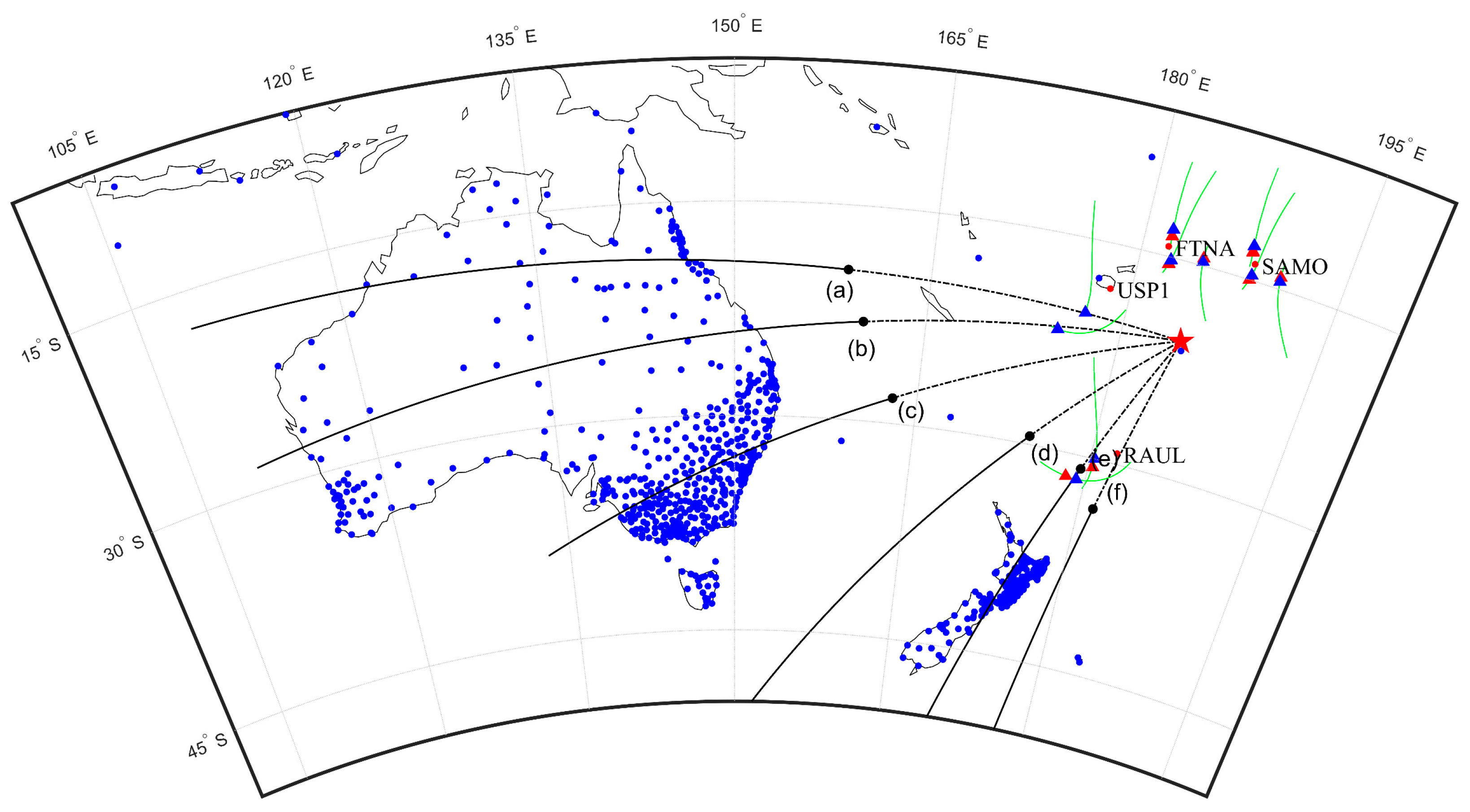
2. Data and Methods

The 2022 Tonga volcanic eruption was preceded by a month of eruptive activity, with the initial explosive eruption occurring on 19 December 2021 [29]. This initial eruption began at 20:40 UT, extending over a duration of 6 h, and generated an ash plume that rose ~13–17 km. The next major volcanic eruption began at 15:20 UT on 13 January 2022, lasted 22 h, and generated an ash plume that rose ~16–20 km [29]. The climactic stage began at 04:15 UT on 15 January 2022 and generated an ash plume that rose higher than 55 km [15]. The climactic eruption generated significant wave perturbations in the upper atmosphere. Our study focused on the ionospheric waves that were induced by the climactic eruption on 15 January 2022. During the climactic volcanic eruptions on 15 January 2022, the Dst index was ~53 nT, and the three-hour averaged Kp index remained below 4, indicating a quiet level of geomagnetic activity. Simultaneously, the number of sunspots was 95, and the F10.7 index measured ~115.6, suggesting low levels of solar activity. Therefore, ionospheric disturbances due to geomagnetic and solar activity were negligible and were not considered in our study.

The GNSS data from the 959 stations used in this paper were obtained from the Geological hazard information for New Zealand and Geoscience Australia GNSS data archive. The GNSS observations contain the phase and pseudo-range of two L-band frequencies with a time resolution of 30 s. Slant TEC ($sTEC$) can be derived from code pseudo-range slant TEC (${sTEC}_P$) and carrier phase slant TEC (${sTEC}_L$) with the following equations:

$$\left\{\begin{array}{c}{sTEC}_P=-{\displaystyle \frac{1}{40.3}}{\displaystyle \frac{{f_1}^2{f_2}^2}{{f_1}^2-{f_2}^2}}\left[\left({P_1-P}_2\right)-c\left(b^{s,1}-b^{s,2}\right)-c\left(b_{r,1}-b_{r,2}\right)\right]\\ {sTEC}_L={\displaystyle \frac{1}{40.3}}{\displaystyle \frac{{f_1}^2{f_2}^2}{{f_1}^2-{f_2}^2}}\left[\left({\lambda }_1{\varphi }_1-{\lambda }_2{\varphi }_2\right)-\left({\lambda }_1{N}_{r,1}^s-{\lambda }_2{N}_{r,2}^s\right)-\left({\lambda }_1{\delta }^{s,1}-{\lambda }_2{\delta }^{s,2}\right)-\left({\lambda }_1{\delta }_{r,1}-{\lambda }_2{\delta }_{r,2}\right)\right]\\ sTEC={sTEC}_L+{\displaystyle \frac{1}{N}}\sum \left({sTEC}_P-{sTEC}_L\right)\end{array}\right.$$

(1)

where $P_1$ and $P_2$ are code pseudo-range measurements at $f_1$ and $f_2$ frequencies, respectively; ${\lambda }_1$ and ${\lambda }_2$ are the wavelengths of $f_1$ and $f_2$ frequencies, respectively; ${\varphi }_1$ and ${\varphi }_2$ are the carrier phase measurements at $f_1$ and $f_2$ frequencies, respectively. $c$ is the speed of light. $b^{s,1}$, $b^{s,2}$, and $b_{r,1}$, $b_{r,2}$ are hardware delays in the satellites and receivers at $f_1$ and $f_2$ frequencies, respectively. $N_{r,1}^s$ and $N_{r,2}^s$ represent integer cycle ambiguity in the carrier phase. ${\delta }^{s,1}$, ${\delta }^{s,2}$, and ${\delta }_{r,1}$, ${\delta }_{r,2}$ are initial phase biases in the satellites and receivers at $f_1$ and $f_2$ frequencies, respectively. Using ${sTEC}_L$ to smooth $s{TEC}_P$, $sTEC$ can be computed. Since the ambiguity terms and initial phase biases are fixed in continuous observations, they can be removed by the phase-smoothed code process. To estimate the hardware delays, we employed the method of Xiong et al. (2019) [30]. We denoted ${sTEC}^{\prime }$ as $sTEC$ after removing the hardware delay. Assuming a thin shell model of the ionosphere, the calculated ${sTEC}^{\prime }$ was projected to the local zenith direction to obtain the vertical TEC ($VTEC$) through a mapping function:

$$\left\{\begin{array}{c}VTEC={\displaystyle \frac{{sTEC}^{\prime }}{SF}}\\ SF={\displaystyle \frac{1}{\sin E_i}}={\displaystyle \frac{1}{\sqrt{1-{\left(\frac{r_e\cos E_0}{r_e+h_m}\right)}^2}}}\end{array}\right.$$

(2)

where $E_i$ is the elevation angle of the satellite at ionospheric piercing points (IPPs), $r_e$ is the radius of the Earth, $h_m$ is the altitude of the thin shell, and $E_0$ is the elevation angle of the satellite at the GNSS station. The altitude of the thin shell was fixed at 300 km, which was the height of ionospheric maximum electron density over New Zealand on 15 January 2022, according to the International Reference Ionosphere model. The cutoff elevation angle was set as 20° to avoid multipath errors and ensure the quality of observations. The TIDs induced by the volcanic eruption had a broad spectral range of frequencies, especially in the near field. Considering that a 30 min window was used for extracting medium- and large-scale TEC perturbations, and given our focus on these scales of perturbations, we utilized 30–50 min Butterworth bandpass filters to derive the differential VTEC (DTEC). Figure 1 shows the geographical locations of the GNSS stations.

We also used brightness temperature data provided by the Japan Meteorological Agency (JMA). Himawari-8 is JMA’s geostationary meteorological satellite located on Earth’s equatorial at 140.7°E. The Advanced Himawari Imager (AHI) carried by Himawari-8 can detect infrared brightness temperature data within the 60°S–60°N × 80°E–20°W region at a 10 min temporal resolution. We used the infrared channel with a central wavelength of 9.6 μm to observe the lower atmosphere oscillations induced by the Tonga volcanic eruptions. This channel has a sensitivity peak at around 40 hPa [31] (at the altitude of ~22 km). The filtering method of brightness temperature data is the same as that of TEC data.

3. Results

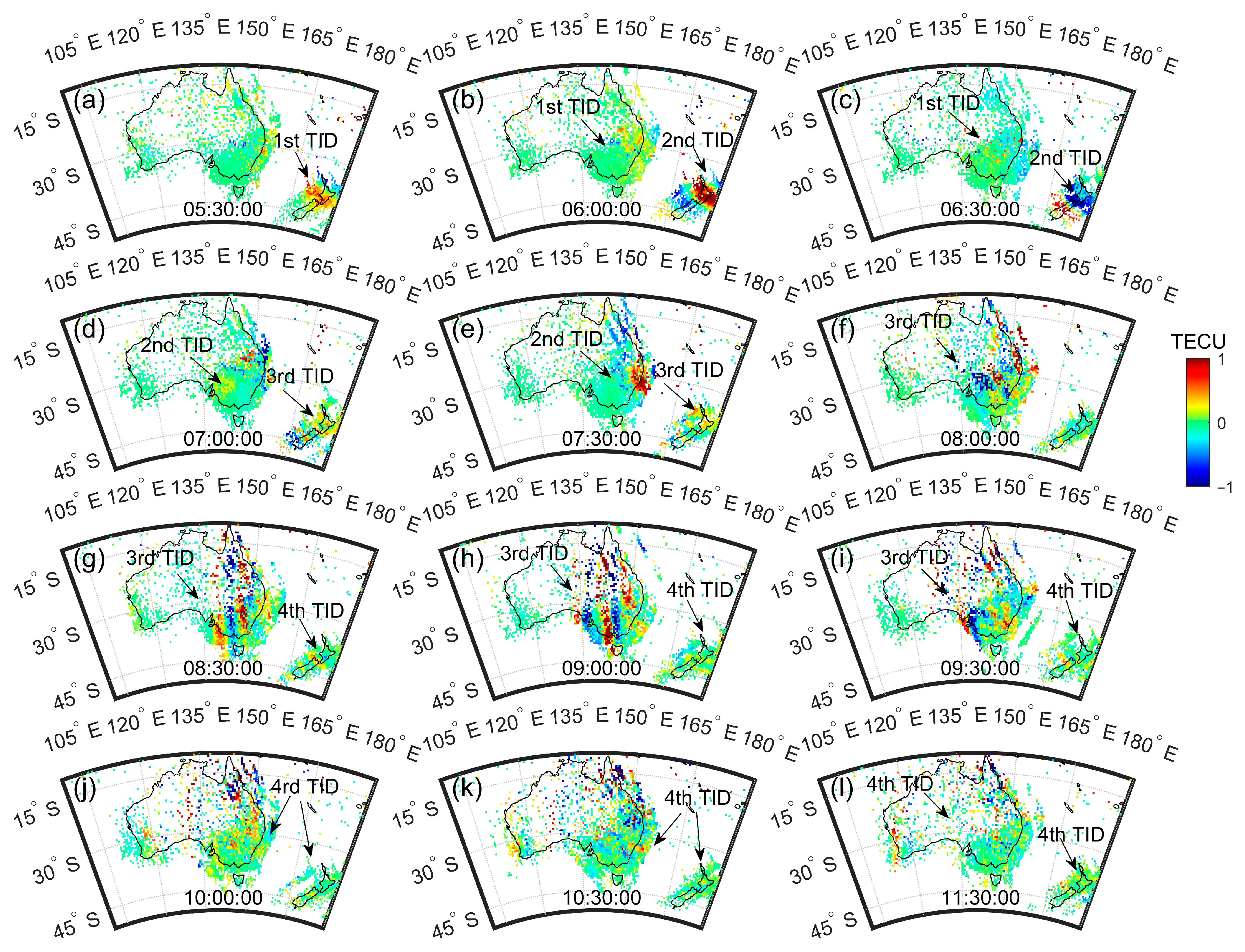
3.1. 2D DTEC Maps of TIDs

Using the GNSS observations across the New Zealand and Australia regions, we constructed two-dimensional (2D) DTEC maps to characterize the TIDs over the near-field regions that were generated by the Tonga volcanic eruption (Figure 2). We identified four groups of TID events following the eruption (labeled 1st TID–4th TID in Figure 2).

The first TID event was observed 45 min after the volcanic eruption. A positive TID structure with an amplitude of 0.6 TECU appeared across northern New Zealand (~1700 km from the eruptive center) at 05:00 UT, with this positive phase front reaching Australia around 05:30 UT and then disappearing ~3500 km from the eruptive center. The second TID event possessed a maximum amplitude of 1.5 TECU and propagated southwestward across New Zealand and Australia before disappearing over Western Australia. The third TID event possessed a relatively narrow wavelength, with an amplitude of ~1.2 TECU. It first appeared across northern New Zealand around 06:30 UT and was then observed propagating 600 km to the southwest within 30 min (Figure 2g,h). The fourth TID event appeared after the third TID and possessed a smaller amplitude and shorter period. This event lasted for a longer duration and gradually disappeared after 16:00 UT. Each of these TID events propagated along the great circle paths from the eruptive center to the New Zealand and Australia regions.

Multiple positive- and negative-phase fronts appeared in the near-field region during 05:00–16:00 UT, thereby making it difficult to distinguish each TID event in the 2D DTEC maps (Figure 2). We replotted DTEC in the time–distance plane to analyze the spatiotemporal variations of the TIDs generated by the volcanic eruptions [32,33,34], as shown in Figure 3.

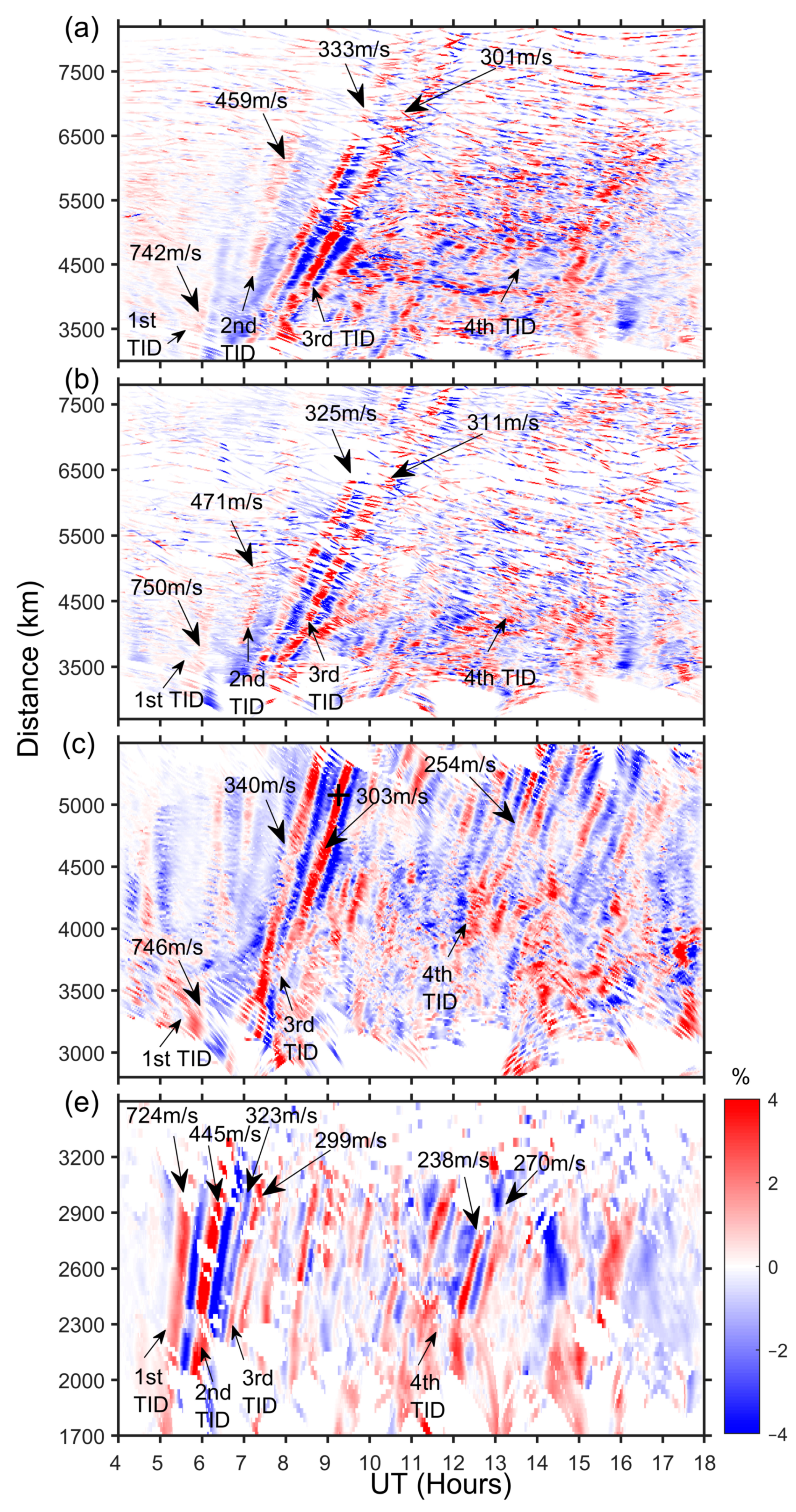
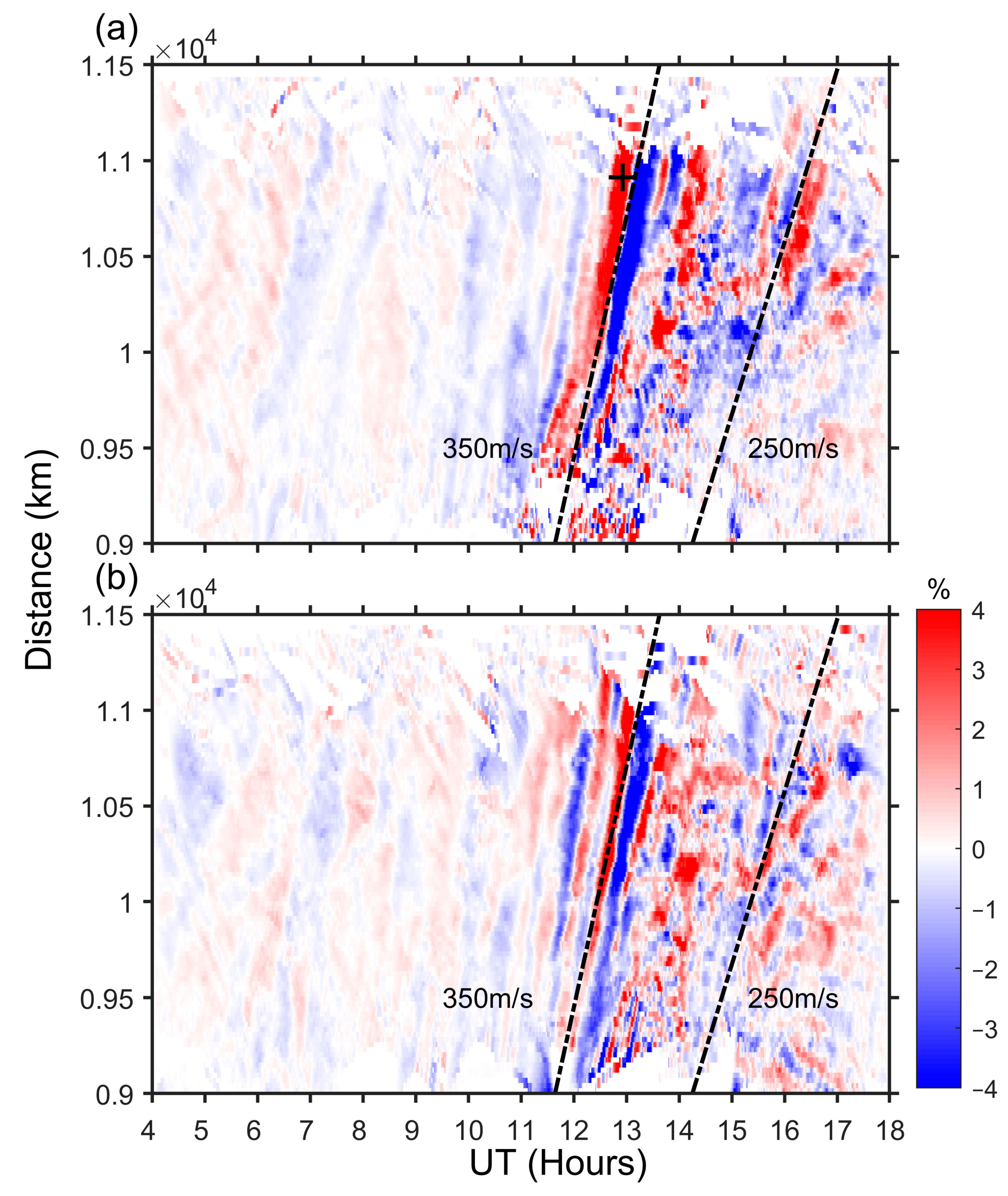
3.2. Keograms of Disturbances

To mitigate the influence of background fluctuations, we utilized relative DTEC (relative deviations between DTEC and JPL-TEC) to represent the amplitude of TIDs. The spatiotemporal variations in relative DTEC along the observational slices are shown in Figure 3. These slices are located along the great circle paths that cross the eruptive center. There appear to be four TID events with different slopes after the volcanic eruption, with each corresponding to a TID event mentioned above.

The first TID event was observed across northern New Zealand at 05:00 UT. The TEC perturbations observed 45 min after the eruption had relative amplitudes of ~4% and velocities of ~724–750 m/s. The disturbance velocity was measured based on the slopes of the phase fronts in the UT–distance plane. Given that the distance between the eruptive center and New Zealand is ~1700 km, it should take about 40 min for a wave to travel from the eruptive center to New Zealand, which basically coincides with the time interval between the eruption time (04:15 UT) and the arrival time of the TID in the New Zealand region (05:00 UT). This disturbance had dissipated after traveling a distance of ~3500 km along the great circle paths (~105 min after the eruption (06:00 UT); Figure 3a–c). The second TID event was observed at 05:30, propagated southwestward along the great circle paths at 445–471 m/s, and had a relative amplitude of ~10%. The second TID event propagated farther than the first one, dissipating by ~6500 km (Figure 3a,b). It took ~166 min for this disturbance to propagate 4500 km at 450 m/s, consistent with the observation result in Figure 3b.

Approximately 2 h and 15 min after the eruption, the third TID event appeared across New Zealand with a relative amplitude greater than 10%. Clear band-like structures with 300–370 m/s velocities and ~38 min periods can be observed between 06:30 and 12:00 UT. The fourth TID event appeared during 07:30–16:00 UT. This disturbance event was characterized by smaller relative amplitudes, shorter periods, and multiple perturbation cycles. The velocity of the fourth TID event was slower than those of the previous three disturbance events, traveling at ~250 m/s. Additionally, whereas the first and second TID events were significantly attenuated during the propagation and disappeared by 3500–6500 km from the eruptive center, both the third and the fourth TID events had almost no attenuation during propagation.

The first and second TID events, which propagated at relatively fast velocities and were rapidly attenuated, were likely associated with shock waves, whereas the third and fourth TID events propagated more than 6500 km with little attenuation (Figure 3a). Previous observations have shown that these latter two TID perturbations surrounded the globe at least three times [15]. The gravity-wave Lamb mode is attributed to these long-distance propagating TIDs.

The energy profiles of ducted modes indicate that the energy of gravity-wave Lamb modes is concentrated on Earth’s surface [35]. To analyze the propagation of Lamb waves in the lower atmosphere, we calculated the brightness temperature variations in the UT–distance plane along slices c–f in Figure 1. Figure 4 presents the spatial and temporal variations in the differential brightness temperature in the infrared channel with a central wavelength of 9.6 μm. The sensitivity peak of this channel is ~22 km [31], which corresponds to the height of the energy peak of the L0 Lamb modes (~20 km) [35]. We positioned the slices in the direction where the disturbance structure was relatively clear. Panels c–f present the brightness temperature observations corresponding to the slices c-f shown in Figure 1. Although the propagation of infrared radiation was affected by clouds and aerosols, the structure of the Lamb waves could still be observed.

The Lamb wave-related disturbances appeared in the brightness temperature observations and then propagated southwestward along the great circle paths between 06:00 and 10:00 UT. These oscillations were characterized by two long-distance propagating phase fronts. The observed Lamb waves propagated at 300–340 m/s, consistent with the TEC-derived velocities of the third TID event (300–370 m/s). In addition, a series of oscillations with small amplitudes and multiple periods appeared after 07:30 UT (Figure 4e,f). These disturbances had a velocity of ~240 m/s, similar to that of the fourth TID obtained from the TEC observations.

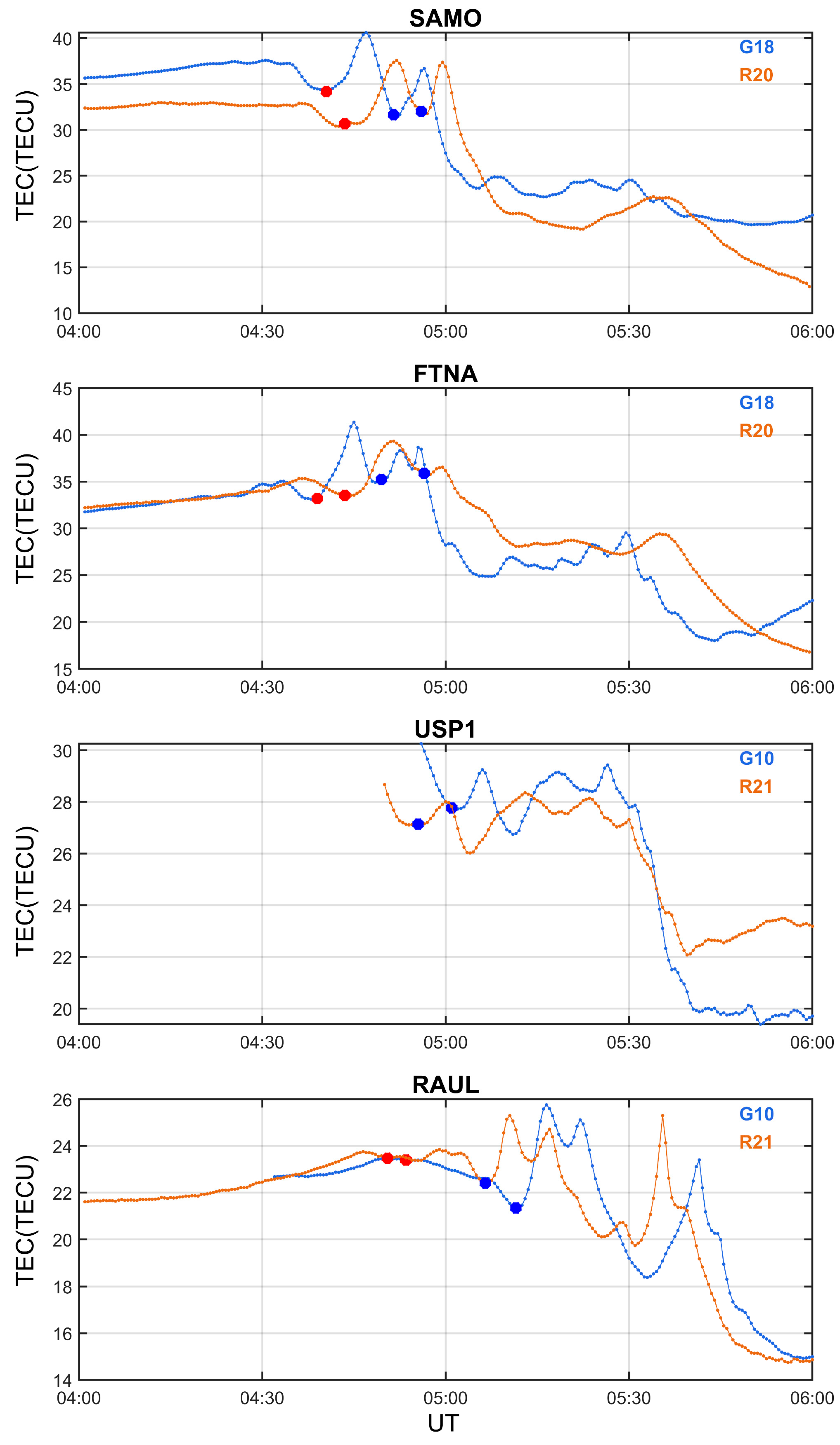
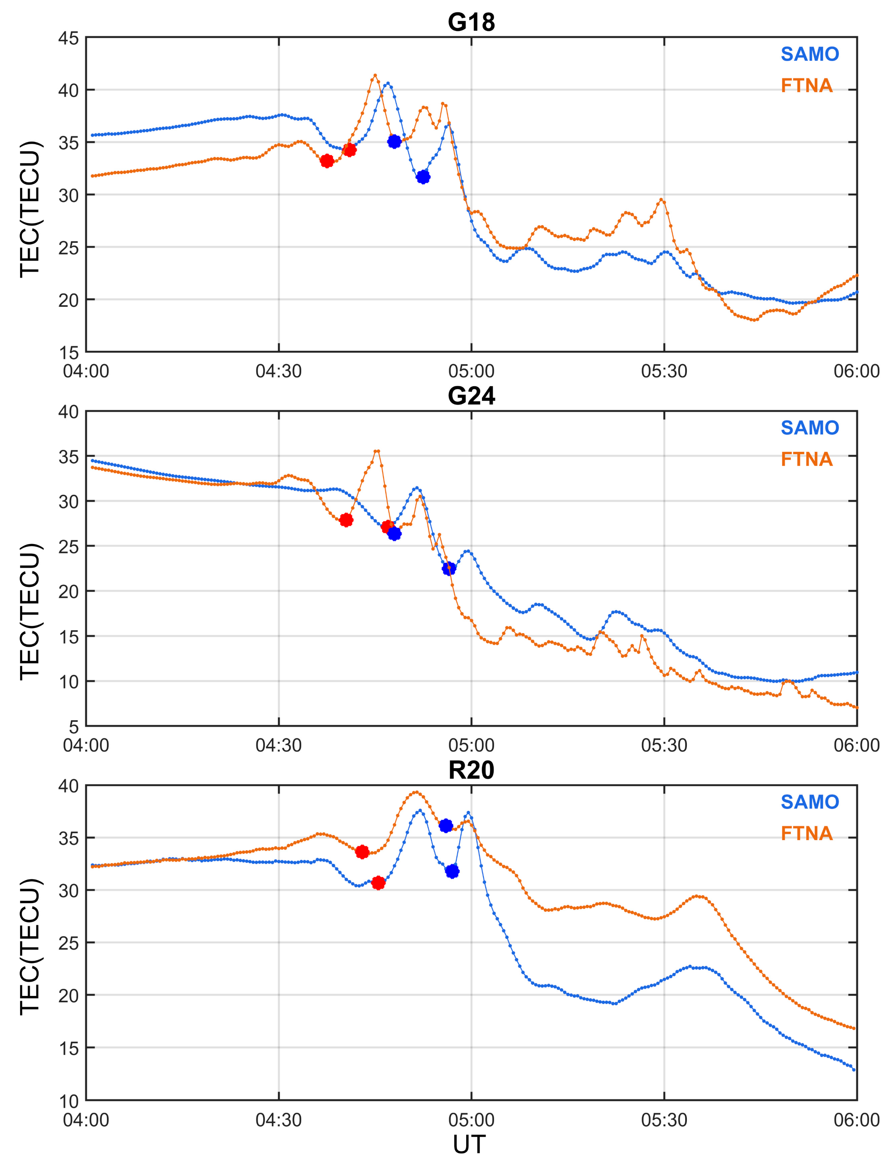
3.3. Onset Times of Multiple Volcanic Explosions

The excitation times of TIDs are bound up with the onset times of volcanic eruptions. A series of explosive eruptions occurred at Hunga Tonga volcano during the December 2021–January 2022 period. The climactic stage of the explosions began on 15 January 2022, with comprehensive satellite- and ground-based observations capturing multiple violent impulsive explosions after 04:00 UT. Different observation data and calculation methods led to varying estimates of the eruption times of the Tonga volcano. According to surface pressure measurements, Wright et al. (2022) identified a series of eruption events between 04:26 UT and 08:46 UT on 15 January 2022 [15]. Vergoz et al. (2022) found that the most intense eruption sequence occurred at ~04:15 UT, peaked at ~04:30 UT, and ended at ~04:40 UT based on seismic, hydroacoustic, and infrasound observations [36]. Astafyeva et al. (2022) estimated five eruption times using TEC data [37]. Maletckii and Astafyeva (2022) proposed a near-real-time method to detect spatiotemporal characteristics of TIDs, estimating four eruption events [38]. Other researchers, such as Robin et al. (2022) [20], Poli and Shapiro (2022) [39], and Tarumi and Yoshizawa (2023) [40], provided different timings based on their methods. These studies highlight that the onset times of the Tonga volcanic eruptions remain subject to debate.

In this section, we calculated the onset times of the Tonga volcanic eruptions and the theoretical propagation velocities of their associated disturbances based on the arrival-time shifts of the TIDs among the TEC observations from adjacent stations. We assumed a rectilinear propagation of the disturbances from the eruptive center to the ionosphere. The perturbation was assumed to propagate at a constant velocity. The onset time of the explosion $T_o$ and theoretical phase velocity $V_t$ can be computed based on the following equations:

$$\left\{\begin{array}{c}\sqrt{{\left({lat}_{\mathrm{i}}-{lat}_S\right)}^2+{\left({lon}_{\mathrm{i}}-{lon}_S\right)}^2+{H_{ion}}^2}=\left(T_i-T_o\right)·V_t\\ \sqrt{{\left({lat}_{\mathrm{j}}-{lat}_S\right)}^2+{\left({lon}_{\mathrm{j}}-{lon}_S\right)}^2+{H_{ion}}^2}=\left(T_j-T_o\right)·V_t\end{array}\right.$$

(3)

where (${lat}_S$, ${lon}_S$, 0) is the point source location; (${lat}_{\mathrm{i}}$, ${lon}_{\mathrm{i}}$, $H_{ion}$) and (${lat}_{\mathrm{j}}$, ${lon}_{\mathrm{j}}$, $H_{ion}$) are the locations of the ionospheric piercing points where the disturbance is detected at times $T_i$ and $T_j$, respectively. We can calculate the onset time $T_o$ and the theoretical phase velocity $V_t$ according to the formula above. The first and second TID events can be identified at most of the stations near the eruptive center owing to their large amplitudes. Figure 5 and Figure 6 show the TEC series used in the calculation. The arrival times of the eruptions are defined as the times when the TEC begins to increase rapidly [15], with the red and blue dots denoting the two major eruption events.

Based on the above method, we determined that two major eruption events occurred at 04:20:54 UT ± 116 s (mean ± the standard deviation; #1) and 04:24:37 UT ± 141 s (#2). These results are consistent with the onset times of the two major eruptions calculated by Astafyeva et al. (04:18:10 UT ± 110 s and 04:26:25 UT ± 100 s, respectively) [37]. The theoretical velocities of the disturbances $V_t$ generated by eruptions #1 and #2 are ~696.9 ± 54.8 and ~503.6 ± 58.3 m/s, respectively. These results coincide with the velocities of the two shock waves estimated from the keograms (724–750 and 445–471 m/s, respectively).

4. Discussion

We identified four TID events propagating across the New Zealand and Australia regions following the Tonga volcanic eruption. The first and second TID events traveled at relatively high speeds (724–750 and 450–471 m/s) and rapidly attenuated as they propagated across the near-field region. These disturbances were caused by the eruption-induced shock waves. The third and fourth TID events propagated at 300–370 and ~250 m/s, respectively. The dispersion curves of ducted waves highlight that the L0 and L1 modes of gravity waves attain horizontal velocities of 311 and 254 m/s, respectively [35]. The third and fourth TID events were caused by the eruption-induced Lamb waves.

The multi-wave structures of TIDs in the near-field region have been reported in previous research. Wright et al. (2022) observed a series of periodic oscillations using multiple instruments across the New Zealand region. The first and second of these TIDs propagated with a velocity of 667 and 414 m/s, respectively [15]. Following the Tonga volcanic eruptions, Tang et al. (2023) detected two broad-wavelength disturbances in New Zealand, with velocities of propagation measured at 643 m/s and 380 m/s [41]. Themens et al. (2022) and Zhang et al. (2022) used dense GNSS observations to identify TIDs traveling across the near-field regions with velocities of ~700 and ~400 m/s [21,22]. These velocities are consistent with those of the shock wave-related TIDs in the present study. Additionally, numerous recent studies have reported TEC disturbances traveling at 300–390 m/s and 200–270 m/s induced by the Tonga volcanic eruption. Ravanelli et al. (2023) identified medium-scale TIDs traveling at ~353 and ~290 m/s across the New Caledonia–New Zealand region [42], while Chen et al. (2023) observed TIDs propagating at 300–330 m/s along the eastern coast of Australia [43]. Tang et al. (2023) reported two narrow-wavelength disturbances traveling across New Zealand with velocities of 358–380 and 252 m/s [41]. The propagation characteristics of these disturbances correspond to the Lamb wave observations in our study. Compared with these previous studies, our research focuses on investigating the excitation characteristics of the shock waves and examining the propagation properties of ducted waves.

4.1. Excitation Characteristics of the Shock Waves

Approximately forty-five minutes following the Tonga volcanic eruption, two shock wave-related TIDs appeared in the TEC observations, traveling at 724–750 and 450–471 m/s, respectively. As illustrated in Figure 3e, these shock wave-related TIDs were severely attenuated as they propagated in the ionosphere, culminating in their disappearance at distances of approximately 3500 and 6500 km from the eruptive center, respectively. The notable difference in the horizontal phase velocities and the propagation distances of two shock wave-related TIDs suggested that their origination could be traced back to distinct volcanic eruptions. Furthermore, the theoretical velocities of the disturbances generated by two major eruptions derived in Section 3.1 are consistent with the shock wave velocities we observed, providing further support for our hypothesis. The relationship between multiple volcanic eruptions and the resultant distinct shock wave-induced disturbances are discussed and verified in this section.

We used the calculated onset times (Section 3.3) and observed shock wave velocities (Figure 3) to estimate the theoretical arrival times $T_t$ of the shock waves generated by the two explosive events.

$$T_t=T_o+{\displaystyle \frac{D}{v}}$$

(4)

where $T_o$ is the onset time of the eruption (04:20:54 UT and 04:24:37 UT), which is calculated via Equation (3); D is the distance from the eruptive center; and $v$ is the observed shock wave velocity (750 and 450 m/s for the first and second shock wave events, respectively). $T_t$ is the theoretical arrival time of shock-related TID induced by each eruption.

Table 1. Comparison of the theoretical (T_t) and actual (T_a) arrival times of the two shock waves.

	D (km)	Tt (UT)		Ta (UT)
		#1	#2
Shock Wave 1	1700	04:58:40	05:02:23	04:58:30
	2300	05:12:00	05:15:43	05:12:00
	2600	05:18:40	05:22:23	05:19:30
Shock Wave 2	2300	05:46:05	05:49:48	05:50:00
	2600	05:57:11	06:00:54	05:59:30
	2900	06:08:18	06:12:01	06:10:30

lists the theoretical arrival times ($T_t$) and the actual arrival times ($T_a$) of the two shock waves.

The theoretical arrival times of the first shock wave induced by eruption #1 coincide with the actual arrival times of the first shock wave (red mark in Table 1), demonstrating a direct link between eruption event #1 and the first shock wave. Similarly, a consistent correlation is observed for the second shock wave with eruption #2 (marked in blue in Table 1). Therefore, we infer that the first shock wave, traveling at velocities of 724–750 m/s, originated from eruption #1 at 04:20:54 UT ± 116 s, while the second shock wave, with velocities of 445–471 m/s, was triggered by eruption #2 at 04:24:37 UT ± 141 s. There is a direct correlation between the multiple volcanic eruptions and the observed shock wave-related TIDs.

4.2. Propagation Mechanisms of the Lamb Waves

The third and fourth TID events with a velocity of 300–370 and 250 m/s appeared following the first two shock wave-related TIDs. Considering their propagation velocities and distances, these two later TID events were caused by GW L0 and L1 modes [18]. The L0 mode with periods of 20–40 min attains horizontal velocities of 311 m/s [35], and velocity deviations of −10 to 60 m/s have been observed in different regions of the world. The observation results in the far-field regions have shown that the Lamb waves on the west coast of North America and the southwest coast of South America possess 365 and 277 m/s velocities, respectively [38]. Kong et al. found that the velocity of Lamb wave-related TID is higher toward the northern hemisphere than toward the southern hemisphere [44]. The velocity anisotropy of the Lamb wave is attributed to the Coulomb force. In addition, the differences in the background atmosphere may induce velocity deviations, as Ding et al. found that background winds and temperature variations could lead to 10–20 m/s variations in the Lamb modes [45].

The comparative analysis of brightness temperature and TEC data suggested that Lamb and shock waves have distinct propagation mechanisms. In the brightness temperature data (Figure 4), disturbances associated with Lamb waves were observed. In contrast, the TEC data (Figure 3) detected both shock waves and Lamb waves. This difference in observed disturbances is due to the distinct propagation mechanisms of these two types of waves. Shock waves are generated by the supersonic ejection of ash plumes and gases during volcanic eruptions. These shock wave-related disturbances, originating near the eruptive center, propagated obliquely upward to the ionosphere and were observed in the ionosphere approximately 8–9 min after the eruption [12]. However, these shock waves did not appear in the brightness temperature data. This is because the infrared channel used for our observations had a sensitivity peak of ~22 km. By the time shock waves reached the regions near New Zealand and Australia, over 1700 km from Tonga, they had already propagated to ionospheric heights. Therefore, the shock waves did not appear in the brightness temperature observations at the lower atmosphere over the New Zealand and Australia regions.

In contrast to shock waves, Lamb waves were identified in both TEC and the lower-atmosphere brightness temperature data. The velocities of Lamb waves in brightness temperature observations (~300–340 m/s and ~240 m/s) were consistent with those in the TEC measurements (~300–370 m/s and ~250 m/s). Lamb waves with periods longer than the upper atmospheric Brunt–Väisälä period (~17 min) are imperfectly ducted [35], leading to energy leakage from the troposphere to the ionosphere. Consequently, both the brightness temperature and TEC data observed Lamb wave-related disturbances. In addition, the arrival times of the Lamb waves in the brightness temperature data were about 10 min earlier than those in the TEC data (Figure 3e and Figure 4e). The timing discrepancy of Lamb waves between the brightness temperature and TEC data reflects the ascent time for wave energy from the lower atmosphere to the ionosphere. Therefore, Lamb waves appeared earlier in the brightness temperature data than in the TEC data. The brightness temperature observations not only demonstrate that Lamb waves maintain a consistent propagation velocity across different altitudes but also validate the fundamentally distinct propagation mechanisms of Lamb waves in contrast to shock waves.

The Lamb wave-related TIDs have almost no attenuation during global propagation. We estimated the relative amplitudes of the Lamb wave-related TIDs observed in China via an approach that was similar to the keogram observations in New Zealand and Australia. The variations in relative DTEC along two slices in China are shown in Figure 7. The distance from the eruptive center to China is about ~9000 km, with panels a and b corresponding to slices a and b in Figure 1 of Li et al. [18]. Considering the South Pacific location of the Tonga volcano, we designate the New Zealand and Australia regions, the continent closest to the Tonga volcano, as the near-field region, and China as the far-field region. The Lamb wave-related TIDs observed in far-field regions have relative amplitudes of ~10.97% (cross in Figure 7a), and those in the near-field region have relative amplitudes of ~11.14% (cross in Figure 3c), with the relative amplitude decreasing by only 0.17% from the near-field region to the far-field region. Therefore, our observation shows that the relative amplitudes of the Lamb wave-related TIDs are approximately constant during this long-distance propagation.

The Lamb waves’ minimal dissipation is attributed to ducting, which has been discussed extensively elsewhere [35,46,47]. Furthermore, since the kinematic viscosity and conductivity increase rapidly above the mesopause, the shock wave-related TIDs would suffer severe attenuation during the propagation. Due to Lamb waves’ and shock waves’ disparate propagation mechanisms, each exhibits distinct attenuation characteristics during their long-distance propagation.

Previous studies have reported both shock wave-related TIDs and Lamb wave-related TIDs triggered by Tonga volcanic eruptions and have also discussed the timing of volcanic eruptions (e.g., shock wave: [20,21,22,23,37,41,42,43]; Lamb wave: [13,18,19,20,21,22,23,28,41,42,43]; and onset times of the Tonga volcanic eruptions: [15,20,36,37,38,39,40]). Our research focuses on the excitation characteristics of shock wave-related TIDs and the propagation mechanisms of Lamb wave-related disturbances. For shock wave-related TIDs, our analysis uniquely demonstrates the direct correlation between multiple volcanic eruptions and specific shock waves. For Lamb wave-related disturbances, we validated the different propagation mechanisms of Lamb waves and shock waves based on observations of brightness temperature and TEC data, noting the differences in their attenuation characteristics. These findings provide observational evidence supporting the theory that Lamb waves and shock waves have fundamentally different propagation mechanisms.

5. Conclusions

Using TEC data from GNSS and brightness temperature data from Himawari-8, the excitation and propagation characteristics of multi-wave TIDs induced by the 15 January 2022 Tonga volcanic eruptions were analyzed. The main conclusions are as follows:

(1)

Two shock waves, with 724–750 and 445–471 m/s propagation velocities, and two Lamb waves, with 300–370 and 250 m/s propagation velocities, were observed in the GNSS–TEC data following the eruptions.

(2)

Based on the time delays of TIDs among the GNSS stations, we estimated the onset times of two major volcanic eruptions, which occurred at 04:20:54 UT ± 116 s and 04:24:37 UT ± 141 s. We inferred and verified that the multiple eruptions corresponded to distinct shock wave-related TIDs.

(3)

Disturbances associated with Lamb waves were identified in both TEC data and brightness temperature measurements, whereas those related to shock waves were not detected in the brightness temperature observations. Furthermore, the Lamb wave-related TIDs exhibited almost no attenuation during global propagation, while the shock waves suffered severe attenuation. These observations indicate that Lamb waves and shock waves have different propagation mechanisms.

References

- Cheng, K.; Huang, Y.N. Ionospheric disturbances observed during the period of Mount Pinatubo eruptions in June 1991. J. Geophys. Res. 1992, 97, 16995–17004. [Google Scholar] [CrossRef]
- Dautermann, T.; Calais, E.; Lognonné, P.; Mattioli, G.S. Lithosphere-atmosphere-ionosphere coupling after the 2003 explosive eruption of the Soufriere hills volcano, Montserrat. Geophys. J. Int. 2009, 179, 1537–1546. [Google Scholar] [CrossRef]
- Dautermann, T.; Calais, E.; Mattioli, G.S. Global Positioning System detection and energy estimation of the ionospheric wave caused by the 13 July 2003 explosion of the Soufrière Hills Volcano, Montserrat. J. Geophys. Res. 2009, 114, B02202. [Google Scholar] [CrossRef]
- Delclos, C.; Blanc, E.; Broche, P.; Glangeaud, F.; Lacoume, J.L. Processing and interpretation of microbarograph signals generated by the explosion of Mount St. Helens. J. Geophys. Res. 1990, 95, 5485–5494. [Google Scholar] [CrossRef]
- Heki, K. Explosion energy of the 2004 eruption of the Asama Volcano, central Japan, inferred from ionospheric disturbances. Geophys. Res. Lett. 2006, 33, L14303. [Google Scholar] [CrossRef]
- Liu, C.H.; Klostermeyer, J.; Yeh, K.C.; Jones, T.B.; Robinson, T.; Holt, O.; Leitinger, R.; Ogawa, T.; Sinno, K.; Kato, S.; et al. Global dynamic responses of the atmosphere to the eruption of Mount St. Helens on May 18, 1980. J. Geophys. Res. 1982, 87, 6281–6290. [Google Scholar] [CrossRef]
- Manta, F.; Occhipinti, G.; Hill, E.M.; Perttu, A.; Assink, J.; Taisne, B. Correlation between GNSS-TEC and eruption magnitude supports the use of ionospheric sensing to complement volcanic hazard assessment. J. Geophys. Res. Solid Earth 2021, 126, e2020JB020726. [Google Scholar] [CrossRef]
- Nakashima, Y.; Heki, K.; Takeo, A.; Cahyadi, M.N.; Aditiya, A.; Yoshizawa, K. Atmospheric resonant oscillations by the 2014 eruption of the Kelud volcano, Indonesia, observed with the ionospheric total electron contents and seismic signals. Earth Planet. Sci. Lett. 2016, 434, 112–116. [Google Scholar] [CrossRef]
- Pekeris, C.L. The Propagation of a Pulse in the Atmosphere. Proc. R. Soc. Lond. 1939, 171, 434–449. [Google Scholar] [CrossRef]
- Shults, K.; Astafyeva, E.; Adourian, S. Ionospheric detection and localization of volcano eruptions on the example of the April 2015 Calbuco events. J. Geophys. Res. Space Phys. 2016, 121, 10303–10315. [Google Scholar] [CrossRef]
- Li, W.; Guo, J.; Yue, J.; Shen, Y.; Yang, Y. Total electron content anomalies associated with global VEI4+ volcanic eruptions during 2002–2015. J. Volcanol. Geotherm. Res. 2016, 325, 98–109. [Google Scholar] [CrossRef]
- Astafyeva, E. Ionospheric detection of natural hazards. Rev. Geophys. 2019, 57, 1265–1288. [Google Scholar] [CrossRef]
- Kubota, T.; Saito, T.; Nishida, K. Global fast-traveling tsunamis driven by atmospheric Lamb waves on the 2022 Tonga eruption. Science 2022, 377, 91–94. [Google Scholar] [CrossRef] [PubMed]
- Omira, R.; Ramalho, R.S.; Kim, J.; González, P.J.; Kadri, U.; Miranda, J.M.; Carrilho, F.; Baptista, M.A. Global Tonga tsunami explained by a fast-moving atmospheric source. Nature 2022, 609, 734–740. [Google Scholar] [CrossRef]
- Wright, C.J.; Hindley, N.P.; Alexander, M.J.; Barlow, M.; Hoffmann, L.; Mitchell, C.N.; Prata, F.; Bouillon, M.; Carstens, J.; Clerbaux, C.; et al. Surface-to-space atmospheric waves from Hunga Tonga-Hunga Ha’apai eruption. Nature 2022, 609, 741–746. [Google Scholar] [CrossRef] [PubMed]
- Aa, E.; Zhang, S.-R.; Erickson, P.J.; Vierinen, J.; Coster, A.J.; Goncharenko, L.P.; Spicher, A.; Rideout, W. Significant ionospheric hole and equatorial plasma bubbles after the 2022 Tonga volcano eruption. Space Weather 2022, 20, e2022SW003101. [Google Scholar] [CrossRef]
- Aa, E.; Zhang, S.-R.; Wang, W.; Erickson, P.J.; Qian, L.; Eastes, R.; Harding, B.J.; Immel, T.J.; Karan, D.K.; Daniell, R.E.; et al. Pronounced suppression and X-pattern merging of equatorial ionization anomalies after the 2022 Tonga volcano eruption. J. Geophys. Res. Space Phys. 2022, 127, e2022JA030527. [Google Scholar] [CrossRef]
- Li, X.; Ding, F.; Yue, X.; Mao, T.; Xiong, B.; Song, Q. Multiwave structure of traveling ionospheric disturbances excited by the Tonga volcanic eruptions observed by a dense GNSS network in China. Space Weather 2023, 21, e2022SW003210. [Google Scholar] [CrossRef]
- Lin, J.-T.; Rajesh, P.K.; Lin, C.C.H.; Chou, M.-Y.; Liu, J.-Y.; Yue, J.; Hsiao, T.-Y.; Tsai, H.-F.; Chao, H.-M.; Kung, M.-M. Rapid conjugate appearance of the giant ionospheric Lamb wave signatures in the northern hemisphere after Hunga Tonga volcano eruptions. Geophys. Res. Lett. 2022, 49, e2022GL098222. [Google Scholar] [CrossRef]
- Robin, S.M.; David, F.; Jelle, D.; Alexandra, M.; David, N.; Keehoon, K. Atmospheric waves and global seismoacoustic observations of the January 2022 Hunga eruption, Tonga. Science 2022, 377, 95–100. [Google Scholar] [CrossRef]
- Themens, D.R.; Watson, C.; Žagar, N.; Vasylkevych, S.; Elvidge, S.; McCaffrey, A.; Prikryl, P.; Reid, B.; Wood, A.; Jayachandran, P.T. Global propagation of ionospheric disturbances associated with the 2022 Tonga volcanic eruption. Geophys. Res. Lett. 2022, 49, e2022GL098158. [Google Scholar] [CrossRef]
- Zhang, S.-R.; Vierinen, J.; Aa, E.; Goncharenko, L.P.; Erickson, P.J.; Rideout, W.; Coster, A.J.; Spicher, A. 2022 Tonga volcanic eruption induced global propagation of ionospheric disturbances via Lamb waves. Front. Astron. Space Sci. 2022, 9, 871275. [Google Scholar] [CrossRef]
- Li, J.; Chen, K.; Chai, H.; Lin, J.; Zhou, Z.; Zhu, H.; Lyu, M. Ionospheric disturbance analysis of the January 15, 2022 Tonga eruption based on GPS data. Sci. China Earth Sci. 2023, 66, 1798–1813. [Google Scholar] [CrossRef]
- Zhou, M.; Gao, H.; Yu, D.; Guo, J.; Zhu, L.; Yang, L.; Pan, S. Analysis of the Anomalous Environmental Response to the 2022 Tonga Volcanic Eruption Based on GNSS. Remote Sens. 2022, 14, 4847. [Google Scholar] [CrossRef]
- He, J.; Astafyeva, E.; Yue, X.; Ding, F.; Maletckii, B. The giant ionospheric depletion on 15 January 2022 around the Hunga Tonga-Hunga Ha’apai volcanic eruption. J. Geophys. Res. Space Phys. 2023, 128, e2022JA030984. [Google Scholar] [CrossRef]
- Hong, J.; Kil, H.; Lee, W.K.; Kwak, Y.-S.; Choi, B.-K.; Paxton, L.J. Detection of different properties of ionospheric perturbations in the vicinity of the Korean Peninsula after the Hunga-Tonga volcanic eruption on 15 January 2022. Geophys. Res. Lett. 2022, 49, e2022GL099163. [Google Scholar] [CrossRef]
- Huba, J.D.; Becker, E.; Vadas, S.L. Simulation study of the 15 January 2022 Tonga event: Development of super equatorial plasma bubbles. Geophys. Res. Lett. 2023, 50, e2022GL101185. [Google Scholar] [CrossRef]
- Harding, B.J.; Wu, Y.-J.J.; Alken, P.; Yamazaki, Y.; Triplett, C.C.; Immel, T.J.; Gasque, L.C.; Mende, S.B.; Xiong, C. Impacts of the January 2022 Tonga volcanic eruption on the ionospheric dynamo: ICON-MIGHTI and Swarm observations of extreme neutral winds and currents. Geophys. Res. Lett. 2022, 49, e2022GL098577. [Google Scholar] [CrossRef]
- Gupta, A.K.; Bennartz, R.; Fauria, K.E.; Mittal, T. Eruption chronology of the December 2021 to January 2022 Hunga Tonga-Hunga Ha’apai eruption sequence. Commun. Earth Environ. 2022, 3, 314. [Google Scholar] [CrossRef]
- Xiong, B.; Li, X.L.; Wan, W.X.; She, C.L.; Hu, L.H.; Ding, F.; Zhao, B.Q. A method for estimating GNSS instrumental biases and its application based on a receiver of multisystem. Chin. J. Geophys. 2019, 62, 1199–1209. [Google Scholar] [CrossRef]
- Zou, X.; Zhuge, X.; Weng, F. Characterization of Bias of Advanced Himawari Imager Infrared Observations from NWP Background Simulations Using CRTM and RTTOV. J. Atmos. Ocean. Technol. 2016, 33, 2553–2567. [Google Scholar] [CrossRef]
- Ding, F.; Wan, W.; Ning, B.; Zhao, B.; Li, Q.; Zhang, R.; Xiong, B.; Song, Q. Two-dimensional imaging of large-scale traveling ionospheric disturbances over China based on GPS data. J. Geophys. Res. Space Phys. 2012, 117, A08318. [Google Scholar] [CrossRef]
- Ding, F.; Wan, W.; Li, Q.; Zhang, R.; Song, Q.; Ning, B.; Liu, L.; Zhao, B.; Xiong, B. Comparative climatological study of large-scale traveling ionospheric disturbances over North America and China in 2011–2012. J. Geophys. Res. 2014, 119, 519–529. [Google Scholar] [CrossRef]
- Ding, F.; Mao, T.; Hu, L.; Ning, B.; Wan, W.; Wang, Y. GPS network observation of traveling ionospheric disturbances following the Chelyabinsk meteorite blast. Ann. Geophys. 2016, 34, 1045–1051. [Google Scholar] [CrossRef]
- Francis, S.H. Acoustic gravity modes and large scale traveling ionospheric disturbances of a realistic, dissipative atmosphere. J. Geophys. Res. 1973, 78, 2278–2301. [Google Scholar] [CrossRef]
- Vergoz, J.; Hupe, P.; Listowski, C.; Le Pichon, A.; Garcés, M.A.; Marchetti, E.; Labazuy, P.; Ceranna, L.; Pilger, C.; Gaebler, P.; et al. IMS observations of infrasound and acoustic gravity waves produced by the January 2022 volcanic eruption of Hunga, Tonga: A global analysis. Earth Planet. Sci. Lett. 2022, 591, 117639. [Google Scholar] [CrossRef]
- Astafyeva, E.; Maletckii, B.; Mikesell, T.D.; Munaibari, E.; Ravanelli, M.; Coisson, P.; Manta, F.; Rolland, L. The 15 January 2022 Hunga Tonga eruption history as inferred from ionospheric observations. Geophys. Res. Lett. 2022, 49, e2022GL098827. [Google Scholar] [CrossRef]
- Maletckii, B.; Astafyeva, E. Near-real-time analysis of the ionospheric response to the 15 January 2022 Hunga Tonga-Hunga Ha’apai volcanic eruption. J. Geophys. Res. Space Phys. 2022, 127, e2022JA030735. [Google Scholar] [CrossRef]
- Poli, P.; Shapiro, N.M. Rapid characterization of large volcanic eruptions: Measuring the impulse of the Hunga Tonga Ha’apai explosion from teleseismic waves. Geophys. Res. Lett. 2022, 49, e2022GL098123. [Google Scholar] [CrossRef]
- Tarumi, K.; Yoshizawa, K. Eruption sequence of the 2022 Hunga Tonga-Hunga Ha’apai explosion from back-projection of teleseismic P waves. Earth Planet. Sci. Lett. 2023, 602, 117966. [Google Scholar] [CrossRef]
- Tang, L. Ionospheric disturbances of the January 15, 2022, Tonga volcanic eruption observed using the GNSS network in New Zealand. GPS Solut. 2023, 27, 53. [Google Scholar] [CrossRef]
- Ravanelli, M.; Astafyeva, E.; Munaibari, E.; Rolland, L.; Mikesell, T.D. Ocean-ionosphere disturbances due to the 15 January 2022 Hunga-Tonga Hunga-Ha’apai eruption. Geophys. Res. Lett. 2023, 50, e2022GL101465. [Google Scholar] [CrossRef]
- Chen, P.; Xiong, M.; Wang, R.; Yao, Y.; Tang, F.; Chen, H.; Qiu, L. On the Ionospheric Disturbances in New Zealand and Australia Following the Eruption of the Hunga Tonga-Hunga Ha’apai Volcano on 15 January 2022. Space Weather 2023, 21, e2022SW003294. [Google Scholar] [CrossRef]
- Kong, Q.; Li, C.; Shi, K.; Guo, J.; Han, J.; Wang, T.; Bai, Q.; Chen, Y. Global Ionospheric Disturbance Propagation and Vertical Ionospheric Oscillation Triggered by the 2022 Tonga Volcanic Eruption. Atmosphere 2022, 13, 1697. [Google Scholar] [CrossRef]
- Ding, F.; Wan, W.; Yuan, H. The influence of background winds and attenuation on the propagation of atmospheric gravity waves. J. Atmos. Solar-Terr. Phys. 2003, 65, 857–869. [Google Scholar] [CrossRef]
- Hunsucker, R.D. Atmospheric gravity waves generated in the high-latitude ionosphere: A review. Rev. Geophys. 1982, 20, 293–315. [Google Scholar] [CrossRef]
- Thome, G.D. Long-period waves generated in the polar ionosphere during the onset of magnetic storms. J. Geophys. Res. 1968, 73, 6319–6336. [Google Scholar] [CrossRef]