Abstract
Temporal oscillations in the IMF Bz associated with Alfvén waves occur frequently in solar wind, with a duration ranging from minutes to hours. Using Swarm observations, Fabry–Pérot interferometer measurements at Mohe station, and Thermosphere–Ionosphere–Electrodynamic General Circulation Model simulations, the perturbations of zonal (ΔUN) and meridional (ΔVN) winds due to temporal oscillations in the IMF Bz on 23–24 April 2023 are explored in the following work. ΔUN is strong westward with a speed of greater than 100 m/s at pre-midnight on 23–24 April. This phenomenon is primarily driven by the pressure gradient, offsetting by the ion drag and Coriolis force. On 23 April, ΔVN is weak northward at the pre-midnight and strong southward at a speed of ~200 m/s at pre-dawn. On 24 April, ΔVN is strong (weak) northward at pre-midnight (pre-dawn). It is mainly controlled by a balance between the pressure gradient, ion drag, and Coriolis force.
1. Introduction
Thermospheric neutral winds are critical in the coupling between the ionosphere and the thermosphere [1,2,3,4,5,6,7]. For instance, in a number of studies, it has been shown that the plasma can be moved along geomagnetic field lines [1,3,4,6], and in the literature, it is also shown that the ionospheric electric field and currents were generated by the collision between ions and neutrals [2]. For instance, the equatorial electrojet could be driven westward/eastward by the eastward winds at Hall/Pedersen altitudes, in association with the collision between ions and neutrals.
During geomagnetic quiet time, the thermospheric neutral winds were shown to have significant local time, longitudinal, hemispheric, seasonal, and solar activity dependences [8,9,10,11,12,13,14,15,16,17,18,19]. Meridional winds are generally equatorward/poleward at nighttime/daytime, and the zonal winds were generally westward/eastward before/after 14 local time (LT) [4,8]. Using the CHAllenging Minisatellite Payload (CHAMP) observations and Thermosphere–Ionosphere–Electrodynamic General Circulation Model (TIEGCM) simulations, Zhang et al. [4] found that the equatorial zonal wind jet at the dip equator blew eastward at 14–06 magnetic local time (MLT) and westward at 06–14 MLT. This windjet has also been studied by Liu et al. [9], Knodo et al. [10], and Miyoshi et al. [11]. They found that the quiet-time windjet is driven by the ion drag, which is related to the electron density and the relative motion between ions and neutrals. Moreover, the equatorial wind jet at 20 MLT increased with the solar activity by approximately 110 m/s and 130 m/s at low and high solar activity. Over the past few decades, a number of researchers have paid attention to the longitudinal pattern of thermospheric winds, e.g., [12,13,14,15,16,17,18]. In their works, the significant wave structures of thermospheric winds have been found. For instance, based on the Fabry–Pérot interferometer (FPI) measurements, Wu et al. [12] revealed that zonal winds may behave differently at different longitudes. They showed that zonal winds observed in Boulder turned westward earlier and had a larger diurnal variation than the zonal winds seen at the Chinese stations during geomagnetic quiet conditions. A strong westward wind at fixed longitudes and 50°–60° GLat was obtained in the CHAMP observations [15]. As reported by Häusler and Lühr [14], Häusler et al. [16], Wang et al. [17], and Wang and Zhang [18], thermospheric winds had an obvious wave-4 longitudinal structure, caused by the strong wave number 3 (DE3) nonmigrating tidal component. The seasonal and hemispheric dependences of the longitudinal pattern of zonal winds were explored in this study by Zhang et al. [13]. They found that the longitudinal distributions of zonal winds in the northern hemisphere were almost the opposite of those in the southern hemisphere. Moreover, the longitudinal patterns during the June solstice were significantly different from those in other seasons. By imposing a poor dipole geomagnetic configuration in the TIEGCM, they found that the geomagnetic field configuration was the main cause of the local time, hemispheric asymmetry, and seasonal changes in zonal winds at middle and low latitudes.
In the literature, the behaviors of neutral winds during the geomagnetically disturbed time have also been investigated, for instance, geomagnetic storms, substorms, and subauroral polarization streams [19,20,21,22,23,24,25,26,27,28]. Dungey [24] suggested in their study that the interaction between the interplanetary magnetic field and geomagnetic field could lead to energy transfer from the solar wind to the Earth’s upper atmosphere. During geomagnetic storm time, the interaction between the southward IMF Bz and geomagnetic field, the energy deposition could lead to the enhancement of Joule heating and neutral temperature and cause large-scale and medium-scale traveling atmospheric disturbances (TADs) in meridional winds [20]. Based on the zonal winds observed by CHAMP, Ritter et al. [24] found that substorm-related disturbed winds increased in the westward with a speed of roughly 50 m/s at midlatitudes around midnight. The universal time (UT) and local time dependences of the substorm effects on zonal winds at high latitudes were explored in this study by Wang et al. [23]. The disturbed winds were poleward and westward in the dusk sector and equatorward and westward at nighttime. The daytime/nighttime perturbation was related to the ion drag/both the Bz and hemispheric power input. Owing to the low background plasma, the disturbed winds responded somewhat later at nighttime than during the daytime. When the geomagnetic pole moved toward the dayside/nightside, stronger/weaker disturbed winds could be generated. Subauroral polarization streams (SAPS) comprised the strong geomagnetic westward plasma flow at the subauroral latitudes [21,26,27,28]. SAPS were located in a latitudinally narrow region from dusk to early morning sectors. SAPS were driven by a strong poleward electric field during geomagnetic disturbed and quiet periods and had a speed greater than 500 m/s. Due to the collision between ions and neutrals, the neutrals were moved westward with ions. At subauroral latitudes, the enhanced frictional heating resulted in the upwelling of molecular-rich air from lower altitudes to higher altitudes. Away from the SAPS region, neutral wind convergent flow produced a downwelling of atomic oxygen-rich air [29]. SAPS-driven nighttime geographic poleward winds at 30°–50° geomagnetic latitudes (MLat) showed obvious UT variations [27]. Due to the misalignment between geomagnetic and geographic coordinate systems, the strong geomagnetic westward ion drag could be separated into two components: geographic poleward/equatorward and geographic westward. The strong geographic poleward ion drag could drive a poleward wind at nighttime and mid-latitudes. Therefore, the poleward wind changes due to SAPS were stronger at 06 and 18 UT and weaker at 00 and 12 UT. By imposing an empirical SAPS model into the global ionosphere thermosphere model, Wang et al. [28] found that the SAPS-driven disturbed winds showed a close correlation with the solar zenith angle χ according to cos0.5 χ; hence, with more sunlight, stronger westward winds were generated. The strongest/weakest disturbed winds occurred on 18/04 and 04/16 UT in the northern and southern hemispheres, respectively.
The authors of previous studies have disclosed that temporal oscillations in the IMF Bz with Alfvén waves are frequent in solar wind [20,30,31]. Liu et al. [30] and Zhang et al. [20] found that the coupled Magnetosphere–Ionosphere–Thermosphere (MIT) system had the nature of a low-pass filter. That is, with respect to the high-frequency IMF Bz, the coupled MIT system could fully respond to the low-frequency IMF Bz. During the geomagnetic storm on 23–24 April 2023, the temporal oscillations in the IMF Bz were strong. However, it is still unknown as to how thermospheric winds would respond to it. The aim of the present study is to address the potential physical drivers and determine the response of thermospheric horizontal winds at Mohe station. In the literature, it is well known that the neutral winds are controlled by a balance between ion drag, pressure gradient, Coriolis force, centrifugal, and viscosity, e.g., [32]. The rapid changes of IMF Bz could lead to perturbations in the ionospheric convection, causing disturbances in the neutral winds via several drivers (e.g., pressure gradient and ion drag). However, when they discuss the roles of IMF Bz on neutral winds, the contributions from IMF Bx and By, solar wind speed, and density cannot be completely excluded. In the present work, we performed two cases: one is input with the observed IMF and solar wind density and speed (real case); the other case is specified by a constant Bz with a value of 0 nT, and the other inputs are the same. In comparison with the previous studies, the effects of solar wind density, wind speed, IMF Bx, and By on neutral winds are removed. Therefore, our findings could improve the understanding of thermospheric winds during the temporal oscillations of IMF Bz. Our study is founded on the previous understanding but does not agree in all parts. Thus, new insights into the neutral wind response to IMF Bz oscillations are revealed.
2. Data and Model Description
Swarm satellites have a near-polar orbit with an inclination of 87°, consisting of three identical satellites: Alpha, Bravo, and Charlie (A, B, and C) [33]. Swarm A and C fly side-by-side at ~450 km, with a 1.4° separation in longitude at the equator. The orbit of Swarm B is ~530 km. The Swarm satellites have an orbital period of ~96 min. The blue lines in Figure 1 indicate the orbits of Swarm A on 23 April. In the present work, the electron density and neutral density measurements from Swarm A were used to estimate the reliability of the TIEGCM. The GRACE-FO twin satellite mission was launched on 22 May 2018. It has been deployed directly to an initial altitude of approximately 520 km, with a near-polar inclination of 89°. Each day, it passes through the Earth 15.3 times. In Figure 1, the orbits of GRACE-FO on 23 April have been indicated by the red lines. In the present work, the cross-track winds from GRACE-FO on 23–24 April 2023 have been used to compare with TIEGCM simulations. We used the Fabry–Pérot interferometer (FPI) operated at Mohe station (122.3° geographic longitude (GLon); 53.5° geographic latitude (GLat)) to aid us in understanding the responses of thermospheric winds to the temporal oscillations in the IMF Bz. The location of Mohe station is indicated by the magenta star shown in Figure 1. The station provides the nighttime wind velocity at around 250 km using the Doppler shift in the airglow in four directions (north, east, south, and west) with an elevation angle of 45°. The FPI observations have a temporal resolution of ~10 min.
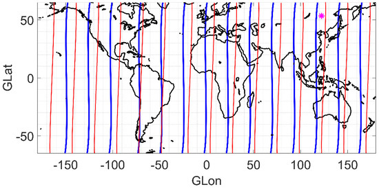
Figure 1.
The orbits of Swarm A (blue line), GRACE (red line), and the Mohe station (magenta star) on 23 April 2023.
The TIEGCM v2.0 is a first principles model of the coupled thermosphere and ionosphere. The drivers include the high-latitude electric field specified by the empirical Heelis model [34] or Weimer model [35], solar EUV, and UV spectral fluxes parameterized by the F10.7 index [36]. In this work, TIEGCM has a horizontal resolution of 2.5° GLat by 2.5° GLon. The vertical resolution is 1/4 scale height, with a bottom/upper boundary of 97/600 km. The lower boundary forcing is specified by either the Global Scale Wave Model (GSWM) [37,38] or the derived tides from the Sounding of the Atmosphere using Broadband Emission Radiometry (SABER) and TIDI observations [12,13]. In the present work, the 1 min IMF data from OMNI was imposed into the TIEGCM with the high-latitude electric field specified by the Weimer model. Note here that the solar wind data from OMNI are observed by the Advanced Composition Explorer (ACE), with the Time-Shifted to the Nose of the Earth’s Bow Shock. The information on ACE can be found at the URL of https://science.nasa.gov/mission/ace/ (accessed on 23 April 2023). The high latitude ion convection and auroral particle precipitation in TIEGCM are defined by the empirical Weimer model [35]. The input parameters for the empirical Weimer model are solar wind density, wind speed, and IMF. The sign of IMF By is changed for the potential pattern in the southern hemisphere. The lower boundary is specified by the migrating and nonmigrating tides from the GSWM model. To reach a diurnally reproducible steady state, the TIEGCM is run for 20 days including the storm event as the last day of the model simulation.
3. Results
3.1. Geomagnetic Conditions
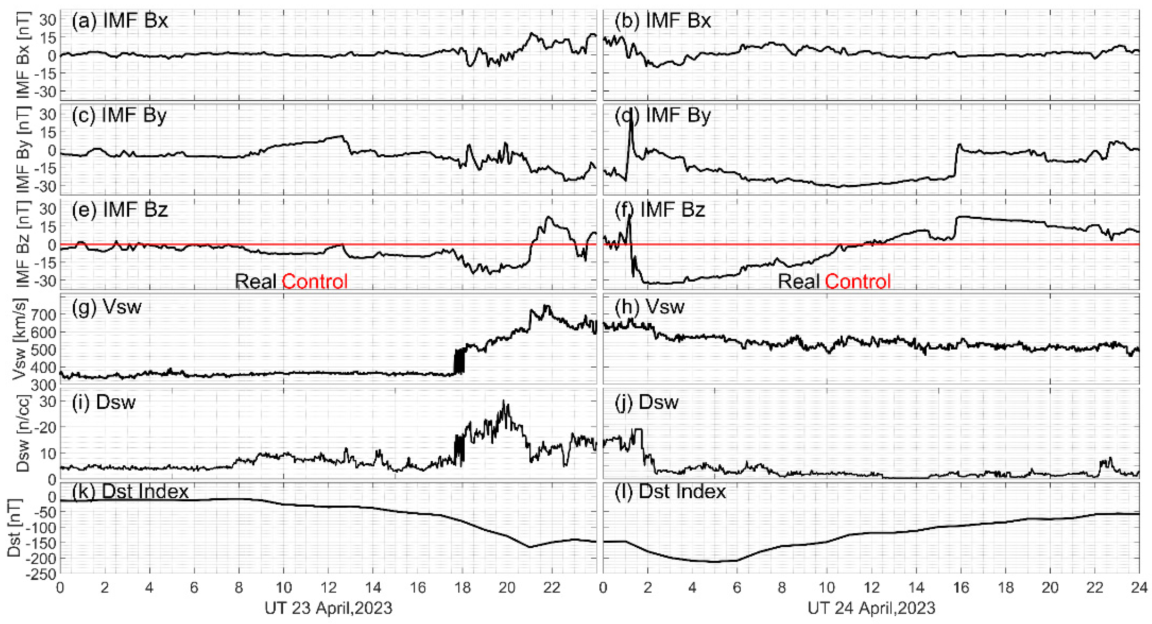
Figure 2 depicts the UT variations in the IMF Bx, By, Bz, solar wind speed (Vsw), wind density (Dsw), and Dst index on 23–24 April 2023. As shown in Figure 2a,b, the IMF Bx varies at around 0 nT at 00–19 UT on 23 April. During the following 7 h, the IMF Bx perturbs greatly with a peak of 26 nT and a trough of −10 nT. After this point, the IMF Bx oscillates at around 0 nT again at 02–00 UT on 24 April. As shown in Figure 2c,d, the IMF By has an average value of −5 nT at 00–12 UT on 23 April. After this point, it increases smoothly to 10 nT at 13 UT on 23 April and quickly decreases to a trough of −31 nT at 11 UT on 24 April. A rapid polarity change is found at 01 UT on 24 April. Figure 2e,f provides the UT variations in the IMF Bz. It can be seen that the IMF Bz varies at around 0 nT at 00–09 UT on 23 April. After this point, the IMF Bz significantly increases southward to −25 nT at 16 UT on 23 April and then turns northward to 25 nT at 23 UT on 23 April. At 03 UT on 24 April, IMF Bz turns southward to a trough of −35 nT. Finally, it turns smoothly northward. In Figure 2e,f, it can be seen that the perturbations of the IMF Bz are significant. According to the results of previous studies [30,31], this may play a critical role in the temporal variations of neutral winds. The real case is treated using the observed IMF Bz imposed in the TIEGCM. To explore the roles of IMF Bz on neutral winds, a control case with a constant Bz of 0 nT is performed in the present work. The differences between the neutral winds in real and control cases are the effects of the temporal oscillations of IMF Bz on neutral winds. In the control case, the inputs (IMF Bx, By, solar wind speed, and wind density) are the same as those in the real case. This indicates that the associated parameters (e.g., convection radius) will be the same between those two cases to exclude their effects on the neutral winds. When a constant IMF Bz with a value of 0 nT is input, the temporal oscillation of the high-latitude ionospheric convection in the real case will be suppressed. This might lead to the suppression of neutral winds, and ionospheric electric field (i.e., prompt penetration electric field and disturbance wind dynamo electric field). However, the detailed behaviors of neutral winds are still unknown. Based on the two cases, the perturbations of neutral winds due to IMF Bz could be analyzed. As shown in Figure 2g,h, Vsw is slow with a speed of less than 400 km/s at 00–17 UT on 23 April. After this point, the Vsw significantly increases to around 700 km/s at 21 UT on 23 April and then maintains at around 500~600 km/s at the remaining UTs. In Figure 2i,j, the Dsw is small with a density of ~5 cm−3 at almost all UTs. At periods from 17 UT on 23 April to 02 UT on 24 April, the density is strong, with a peak of 30 cm−3 at 20 UT. In Figure 2k,l, the Dst index decreases slowly from 0 nT at 00 UT on 23 April to a trough of approximately −200 nT at 05 UT on 24 April. After 05 UT, the Dst index finally recovers to around −50 nT at 00 UT on 25 April.
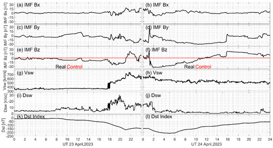
Figure 2.
The UT variations of IMF Bx (top panel), By (second panel), Bz (third panel), the solar wind speed (fourth panel, Vsw) and density (fifth panel, Dsw), and Dst index (bottom) on 23–24 April 2023. The red line in the third panel is the control case.
3.2. Data–Model Comparison
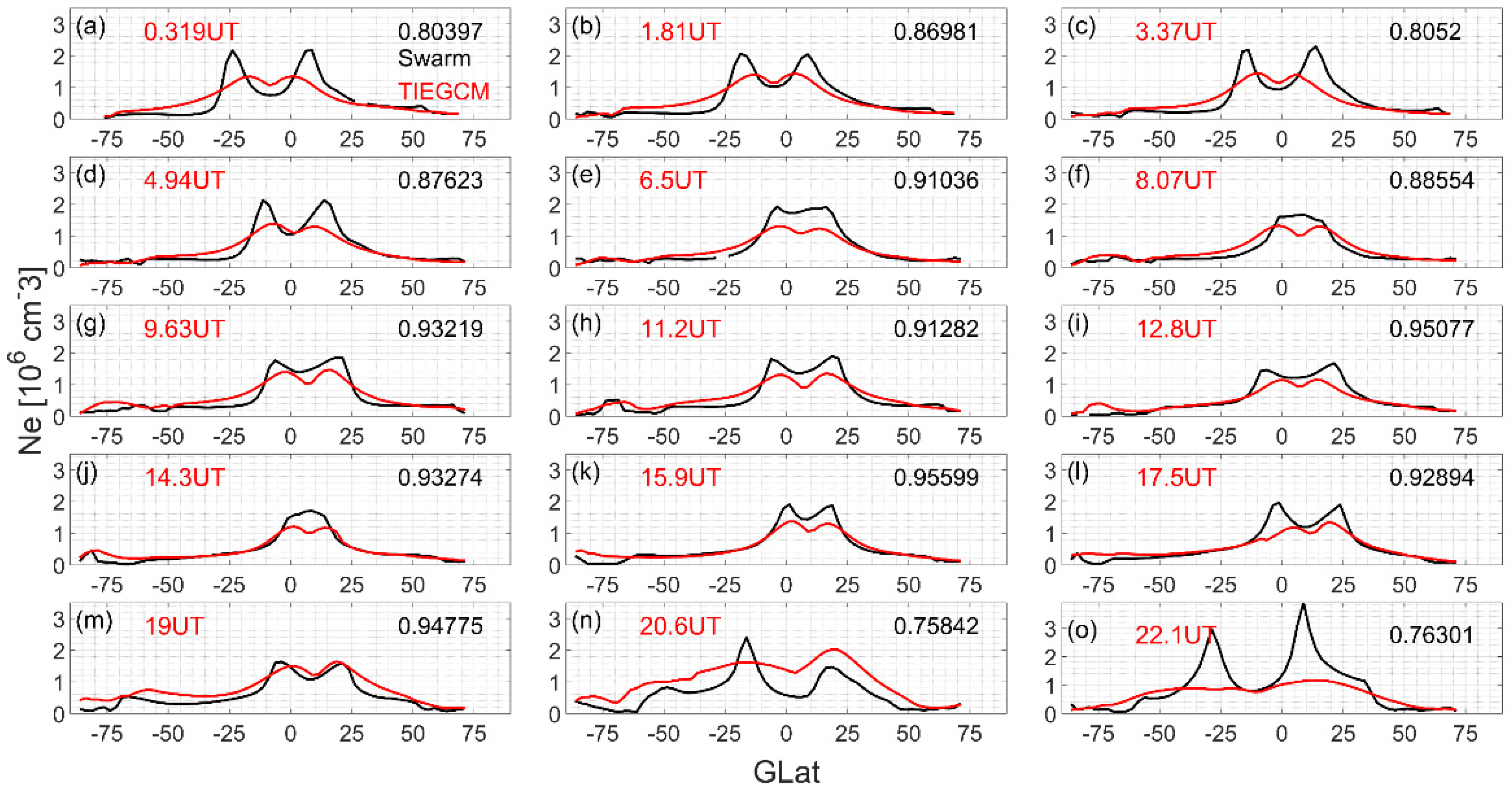
Figure 3 illustrates the latitudinal profiles of the Swarm A observed electron density (Ne) at ~450 km on 23 April 2023. As shown in Figure 3a, Swarm A observed Ne at 0.319 UT on 23 April has a pronounced two-peak structure at low latitudes. The southern and northern peaks are located at −25° GLat and 5° GLat, with a density of 2.1 × 10⁶ and 2.0 × 106 cm−3, respectively. This is the equatorial ionization anomaly (EIA), which is related to the daytime equatorial fountain [39,40]. The equatorial fountain is a phenomenon in which the daytime equatorial plasma moves upward to a high altitude for the eastward electric field, and then downward along the magnetic field line to form the ionization crest at EIA latitudes. A prominent two-peak structure is also found in the TIEGCM-modeled Ne. Note that the TIEGCM modeled Ne is binned at the corresponding GLat, GLon, and UT to the Swarm A data. The northern and southern peaks occur at 1° GLat and −20° GLat, with a density of 1.5 × 10⁶ and 1.5 × 106 cm−3, respectively. The correlation coefficient between Swarm A observed and the corresponding TIEGCM modeled Ne is 0.80397. However, at low latitudes, the prominent two peak structure is underestimated by the model, and the correlation coefficient between modeled and observed Ne is 0.40727. This might be related to the underestimation of neutral winds by TIEGCM, e.g., [4]. The plasma could be moved upward along the geomagnetic fields by the neutral winds, including equatorward winds and zonal winds. When the neutral winds are underestimated, the modeled electron density at EIA latitudes is not very consistent with the observations. Thus, the above results indicate that the large-scale structure of observed Ne is partially reproduced by TIEGCM. At 1.81–22.1 UT on 23 April (Figure 3b–o), the correlation coefficient ranges from 0.75842 to 0.95599. This result confirms the reasonability and reliability of the model in capturing the temporal variations of Ne.
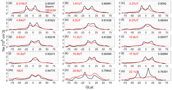
Figure 3.
The latitudinal profile of Swarm A observed and TIEGCM modeled electron density (Ne) at ~450 km on 23 April 2023. (a–o) are for dayside Ne at different Swarm orbits on 23 April. The black and red lines are for Swarm observations and TIEGCM simulations, respectively. The red number on the left hand is the average UT of Swarm orbit. The black number is the correlation coefficient between TIEGCM simulations and Swarm observations. Ne is given in 106 cm−3.
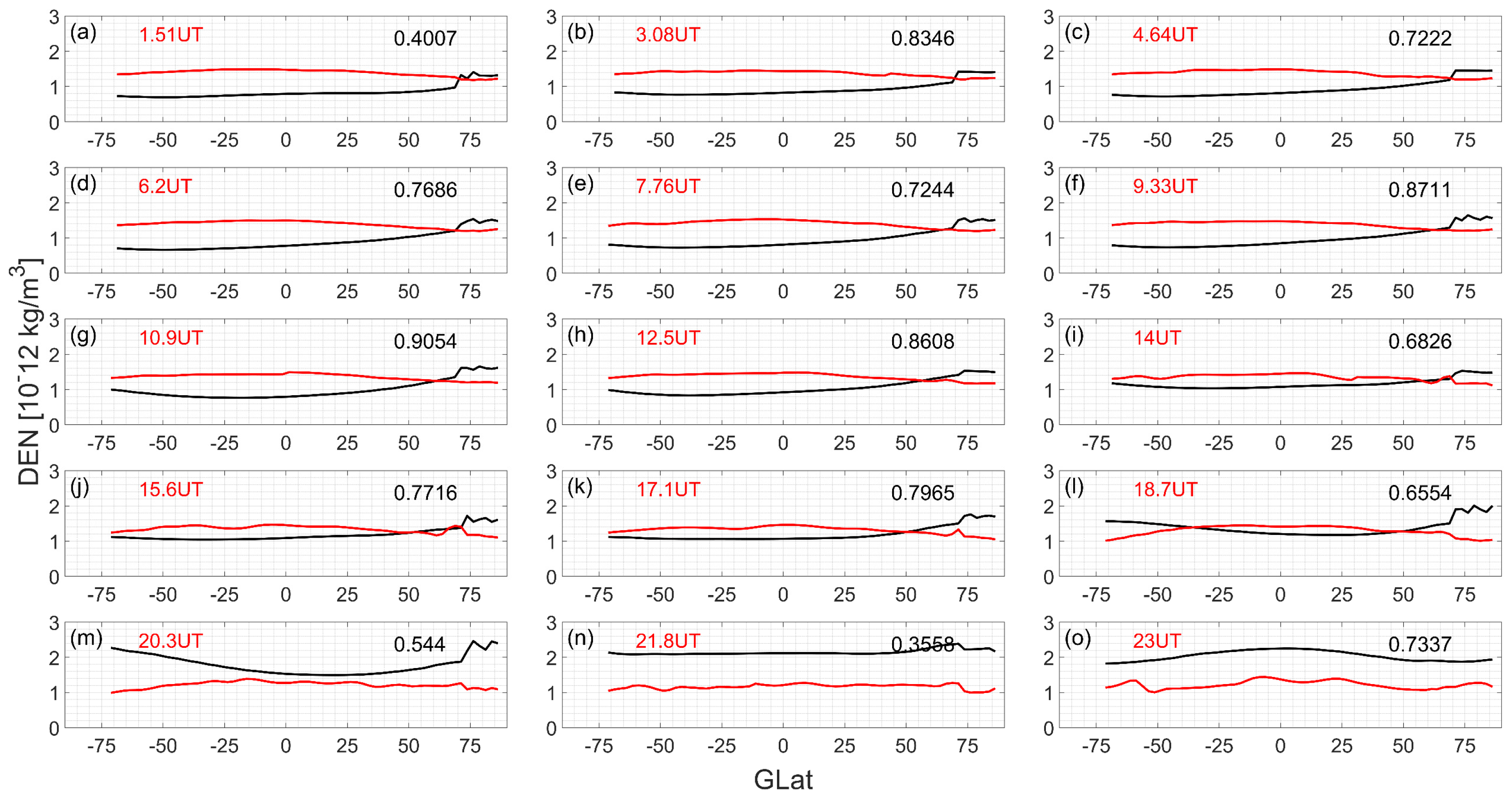
Figure 4 gives the latitudinal profiles of the Swarm observed and TIEGCM modeled neutral density (DEN) on 23 April 2023. In Figure 4a, the Swarm observed DEN at middle and low latitudes has an average density of about 1.0 × 10⁻¹² kg/m3 at almost all latitudes at 1.5 UT. However, the corresponding modeled DEN is stronger than the observations. It has an average density of 1.3 × 10⁻¹² kg/m3. This result is also obtained at the following 10 orbits, from 1.5 UT to 17.1 UT (Figure 4b–k). The correlation coefficient between observations and simulations is larger than 0.5 in almost all orbits, ensuring the reliability of the model. The unexpected orbits occur in Figure 4a,n, with a coefficient of 0.4007 and 0.3558, respectively. As shown in Figure 2, at 17 UT, the solar wind density, wind speed, and IMF Bz start to perturb significantly. Therefore, in Figure 4l–o, the average observed DEN is significantly enhanced to around 2.0 × 10⁻¹² kg/m3. In comparison, the modeled DEN has an average density of 1.5 × 10⁻¹² kg/m3. Thus, it can be seen that the modeled DEN is slightly weaker than the observations. The increase of modeled DEN is slower than the observed DEN. The discrepancy between observations and simulations does not affect the reasonability and reliability of the model. Because the large-scale patterns of observed DEN are well captured in the modeled results. Furthermore, the correlation coefficient between simulations and observations is larger than 0.5 in almost all the orbits. This also confirms the above conclusion.
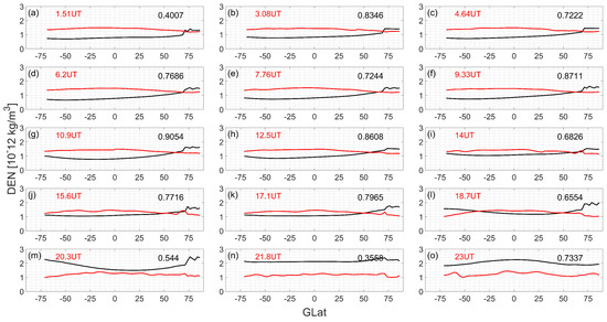
Figure 4.
Similar to Figure 3, but for the neutral density (DEN) on 23 April 2023. (a–o) is for DEN at different dayside Swarm orbits on 23 April 2023. DEN is given in 10−12 kg/m3. The black and red lines are for Swarm observations and TIEGCM simulations, respectively. The correlation coefficient is given on the right side.
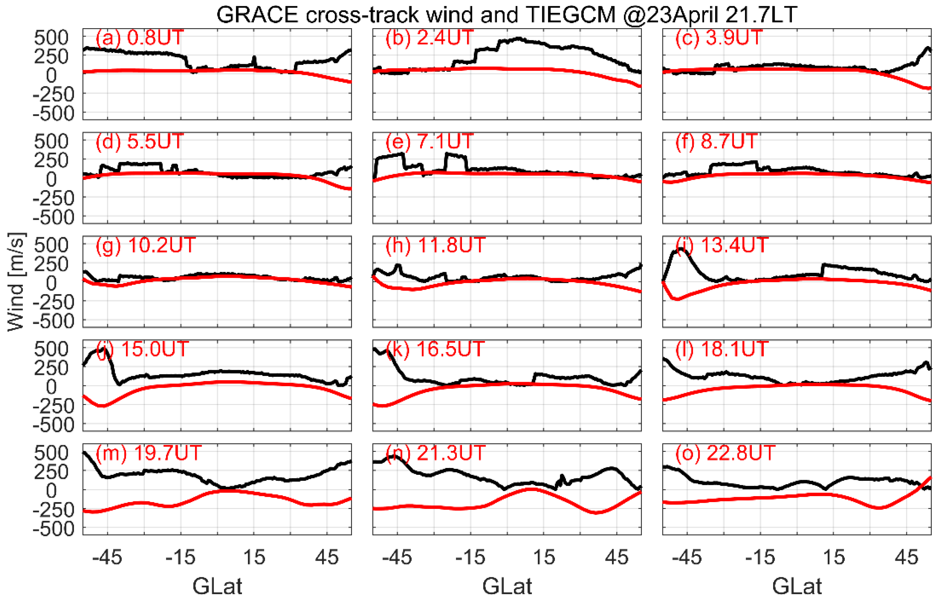
Figure 5 shows the latitudinal profiles of GRACE observed and TIEGCM modeled zonal winds at 21.7 LT on 23 April. Because of the near-polar orbit of GRACE, the cross-track winds at middle and low latitudes can be treated as zonal winds. In Figure 5a, the observed cross-track winds decrease smoothly from around 250 m/s at southern middle latitudes to around zero m/s in the equatorial region and increase to around 200 m/s at the northern middle latitudes. The modeled zonal winds have an average speed of 34 m/s. The winds are underestimated by the model, which has been disclosed by a number of previous studies, e.g., [13]. However, the large-scale pattern of zonal winds at middle and low latitudes has been partially captured by the TIEGCM, ensuring its reliability. Moreover, in the literature, the behaviors of zonal winds during storms and quiet times have been explored using TIEGCM, e.g., [4,12,32]. A similar large-scale structure between observations and simulations is also obtained in Figure 5b–o.
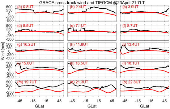
Figure 5.
Similar to Figure 3, but for the GRACE observed cross-track winds on 23 April 2023. (a–o) is for winds at difference GRACE orbits at dayside on 23 April. The black and red lines are for GRACE observations and TIEGCM simulations, respectively. The cross-track winds are given in m/s.
In Figure 3, Figure 4 and Figure 5, the observed Ne, neutral density, and zonal winds seem to be not accurately captured by the TIEGCM. This finding may be related to the following two factors. One pertains to the resolution of the TIEGCM, and the other concerns the high-latitude electric field specified by the empirical Weimer model. As reported by previous studies [15], small-scale electric field variability and ion-electron collisional heating cannot be entirely captured by large-scale physical models, including the TIEGCM. The TIEGCM has a horizontal resolution of 2.5° GLat × 2.5° GLon, with a vertical resolution of a quarter scale height. In the ionosphere, a grid of 2.5° GLat × 2.5° GLon indicates a spatial scale larger than 200 km. Therefore, the small-scale variability and ion-electron collisional heating cannot be fully reproduced. In the present work, the high-latitude electric field is calculated based on the 1 min solar wind data. The method may not be sufficient for gaining an accurate representation of the ionospheric convection. However, large-scale structures of observed Ne and TEC share a high degree of similarity with that in TIEGCM simulation. Therefore, the minor discrepancy between the observations and simulations is acceptable in the model work.
3.3. Neutral Wind at Mohe Station
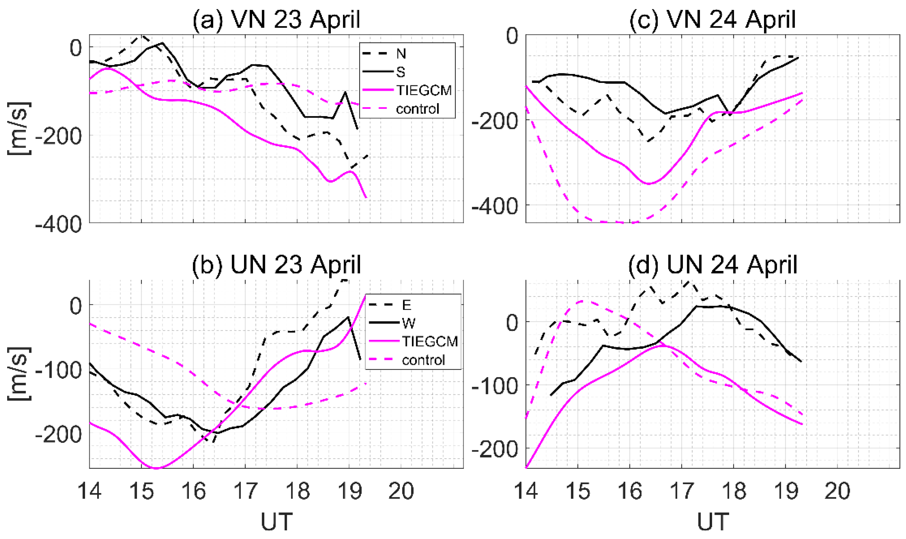
Figure 6 provides information on the temporal variations of the observed nighttime horizontal neutral winds on 23–24 April from the FPI operated at Mohe station. As shown in Figure 6a, the observed meridional winds (VN) on 23 April 2023 are enhanced equatorward from −10 m/s at 14 UT to around −300 m/s at 19.50 UT. Note here that the negative sign stands for the equatorward winds. The modeled VN is smoothly enhanced equatorward from about −50 m/s at 14 UT to −350 m/s at 19 UT. The correlation coefficient between the modeled and observed VN is 0.9313, with a root mean square error of 70.4870 m/s. As shown in Figure 6c, on 24 April, both the observed and modeled VN yield a structure similar to “V”, with troughs of −250 and −350 m/s at 16:30 UT, respectively. The observed VN is −100 and −50 m/s at 14 and 19 UT, respectively. In comparison, the modeled VN is −100 and −120 m/s at 14 and 19 UT, respectively. The correlation coefficient is 0.93352, with a root mean square error of 61.5069 m/s. The strong decrease of meridional winds at around 16 UT is controlled by both the pressure gradient and Coriolis force. The Coriolis force is related to the Coriolis coefficient and the zonal winds. At Mohe station, the coefficient is constant, and the westward winds decrease from 14 UT to 16 UT (Figure 6d). Therefore, the effects of the Coriolis force decrease with time. The interaction between the southward Bz (Figure 2f) and the geomagnetic field leads to the energy transfer from the solar wind to the upper thermosphere. The heated air at high latitudes would travel to the middle latitudes, with a time delay. It might be concluded here that the strong decrease of meridional winds is induced by both the pressure gradient and Coriolis force. In Figure 6a,c, a conclusion could be reached whereby the large-scale temporal variations in VN are suitably captured by the TIEGCM, with minor differences in the speed. The discrepancy in speed does not affect the reliability and reasonability of the model, which is acceptable in the model work [7,29,39]. Therefore, it is possible to use the TIEGCM to explore the responses of VN during the geomagnetic storm on 23–24 April 2023. In the control case, the meridional winds in equatorward have an average speed of approximately 100 m/s, which is much weaker than that in the real case. This indicates that the IMF Bz plays an important role in the formation of strong equatorward winds on 23 April. However, on 24 April, the equatorward winds between the two cases are opposite. This might be related to the weakened energy deposition under the northward IMF Bz (Figure 2f). Moreover, on 23 April, the orbits of GRACE fly through the Mohe station at 13.4 UT (Figure 5i,1). In Figure 5i, the GRACE observed cross-track winds have an average speed of 17.62 m/s. The FPI observed winds at 14 UT and Mohe station have a speed of approximately −10 m/s. The magnitude of winds is comparable between FPI and GRACE observations. The differences in magnitude and direction are acceptable because of the time gap and the longitude and latitude differences between the GRACE orbit and the FPI station.
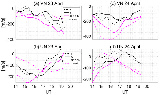
Figure 6.
The UT variations of FPI observed nighttime horizontal winds at Mohe station on 23–24 April 2023. The top-to-bottom panels are for meridional (VN) and zonal (UN) winds, respectively. Black (dotted and solid) and magenta lines are observed and modeled as neutral winds, respectively. The magenta dotted line is the modeled neutral winds in the control case. Both the meridional and zonal winds are given in m/s (positive for poleward and eastward). ‘N’, ‘S’, ‘W’, and ‘E’ are the four directions of airglow observations (N: north, S: south, W: west, E: east).
Figure 6b,d shows the temporal variations of UN at Mohe station during the geomagnetic storm on 23–24 April 2023. As shown in Figure 6b, on 23 April, the FPI observed UN forms a structure similar to the letter ‘V’ as well. The trough of UN is found at approximately 16.5 UT, with a velocity of −210 m/s. The negative velocity is the westward winds. At 14 UT, the observed UN is westward at a speed of 100 m/s. At 19 UT, the observed UN is weak eastward at a speed of about 50 m/s. As indicated by the magenta line, the modeled UN increases westward from −200 m/s at 14 UT to −270 m/s at 15.5 UT and then accelerates eastward to 10 m/s at 19 UT. In comparison with the observed UN, the temporal patterns of the modeled UN from the TIEGCM share a high degree of similarity. The correlation coefficient is 0.8440, with a root mean square error of 145.53 m/s. As shown in Figure 6d, both modeled and observed UN on 24 April show a structure similar to a reverse ‘V’. The peaks of modeled and observed UN appear at 16.5 and 17 UT, with a velocity of −30 and 30 m/s, respectively. In summary, it is possible to confirm the reliability and reasonability of TIEGCM in capturing the dynamics of thermospheric zonal winds, as shown in Figure 6b,d.
In the TIEGCM, the calculation of neutral winds is based on the momentum Equations (1) and (2).
In Equations (1) and (2), is the meridional winds, is the zonal winds, Re is the Earth’s radius, is the geographic latitude, is the altitude, is the molecular viscosity, and and are the ion drag coefficients. The forcing terms are in this order: the vertical viscosity (the second term), Coriolis force (the third term), ion drag (fourth and fifth terms), nonlinear horizontal advection (the sixth term) and momentum force (the seventh term), pressure gradient (the eighth term), vertical advection (the ninth term), and horizontal diffusion (the tenth term). Therefore, the effects of each force on the neutral winds could be expressed by the accelerations, that is, the term analysis in the TIEGCM. When the input IMF Bz changes, the described high-latitude electric field would change. For instance, the two-cell pattern is generated under southward Bz. However, under northward Bz, the high-latitude convection is complicated (i.e., four-cell pattern). The high-latitude convection perturbations in the TIEGCM could lead to the changes of neutral temperature via Joule heating. The heated air could travel to the middle and low latitudes, causing TADs in thermospheric winds. Moreover, the high-latitude convection could also produce perturbations in the ionospheric electric field and electron density. This could drive a disturbance in the thermospheric winds through the ion drag effects. Therefore, the input (IMF Bz) changes could potentially produce significant perturbations in the output (neutral winds). However, the detailed roles of IMF Bz on neutral winds at Mohe are still unknown and deserved to be explored using TIEGCM.
In Figure 6, the general trend of neutral winds has been well reproduced by the TIEGCM. However, the significant 90–120 min periodicity is not well captured by the model. This might be related to the deficiency in the high-latitude drivers. The high-latitude electric field in the TIEGCM is specified by the empirical Weimer model [35]. This widely used Weimer ion convection model is derived from the Dynamic Explorer 2 (DE2) data set and parametrized by solar wind conditions and Earth’s dipole tilt angle with respect to the Sun for opposite hemispheres. It describes the average high-latitude ionospheric conditions that generally do not fully describe the actual spatial and temporal variations of neutral winds.
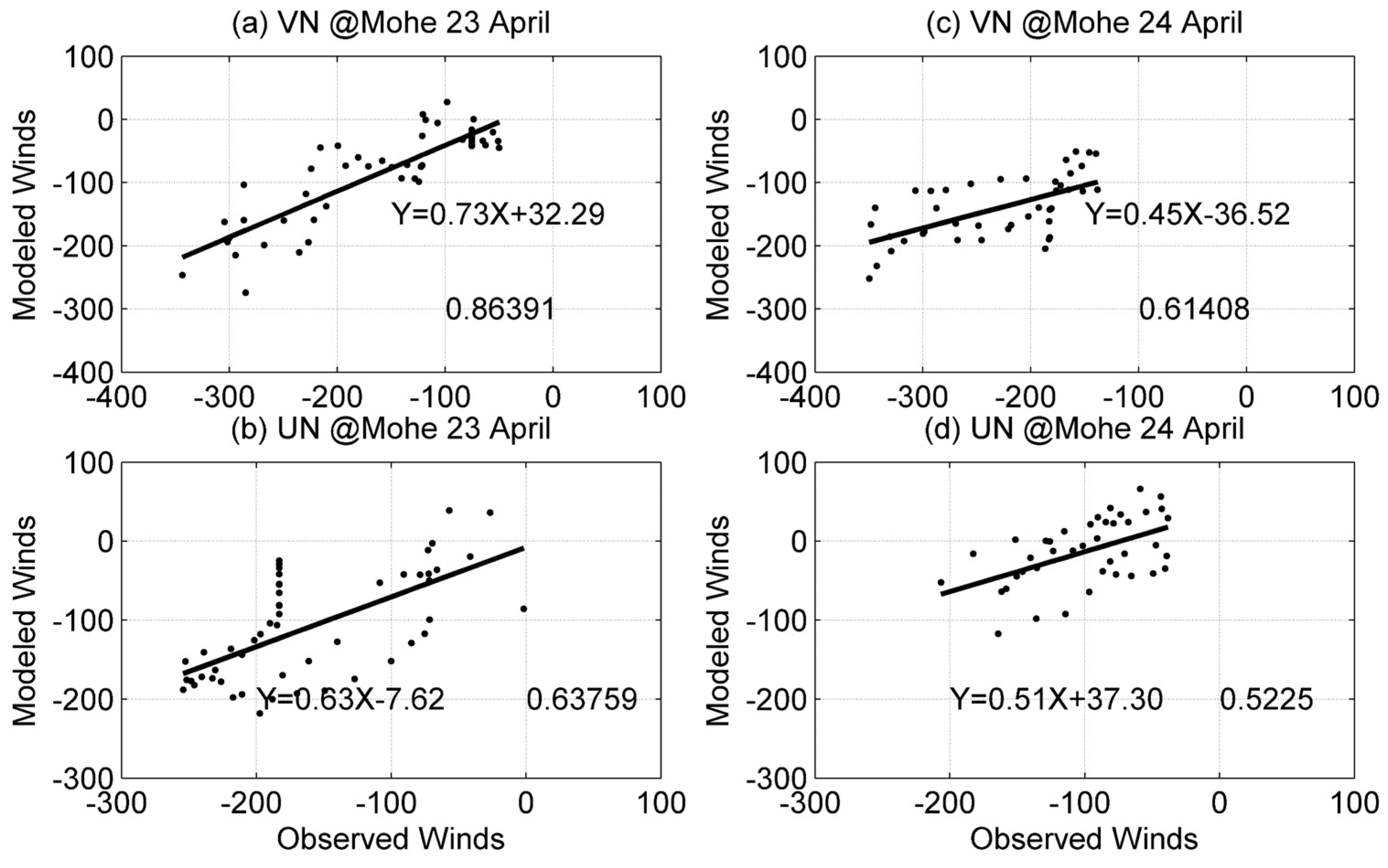
To identify the reliability of the TIEGCM, a scatter plot of the modeled and observed zonal and meridional winds at nighttime at Mohe station is shown in Figure 7. As shown in Figure 7a, the modeled meridional winds on 23 April have a good agreement with the observed winds. The correlation coefficient between these two is 0.86391, ensuring the reliability of model. The regression line has a slope of 0.73. On 24 April (Figure 7c), a similar conclusion could be achieved, with the correlation coefficient of 0.61408 and the slope of 0.45. In Figure 7b,d, the correlation coefficient between the modeled and observed zonal winds is 0.63759 and 0.5225 on 23 and 24 April, respectively. The slope of the regression line is 0.63 and 0.51, respectively. Therefore, the reliability of the model in capturing the dynamics of neutral winds could be confirmed.
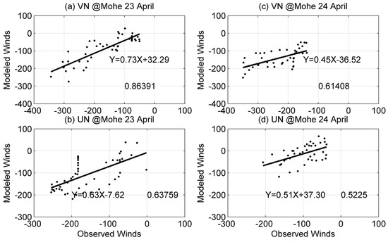
Figure 7.
The scatter plot of the modeled and observed winds at Mohe station. The top-to-bottom panels are the meridional and zonal winds, respectively. The left-to-right columns are the winds on 23 and 24 April, respectively. The winds are given in m/s. The correlation coefficient is given on the right side. The black lines with equations are the regression lines.
4. Discussion
During the geomagnetic storm, the interaction between southward IMF and the geomagnetic field leads to the occurrence of open field lines [24]. The charged particles in the solar winds enter the Earth’s upper thermosphere along the open field lines, causing energy deposition and momentum transfer. High-latitude ionospheric convection and Joule heating constitute significant changes. Joule heating could enhance the neutral temperature, and the disturbances in the thermosphere could travel to the middle and low latitudes, causing traveling atmospheric/ionospheric disturbances (TADs/TIDs). The traditional TADs are equatorward. However, unexcepted poleward TADs/TIDs at middle latitudes have been observed by researchers, including Zhang SR et al. [41]. As described in the literature, the behavior of neutral winds is controlled by a balance between pressure gradient, ion drag, Coriolis force, centrifugal, and viscosity [4,11,32]. The issue is that the potential drivers of neutral wind changes at Mohe station during the strong temporal oscillations in the IMF Bz are still unknown. As we discussed before, the pressure gradient in association with the neutral temperature would be greatly influenced by the IMF Bz oscillations. Furthermore, during IMF Bz oscillations, the prompt penetration electric field (PPEF) and ion drifts at middle and low latitudes are disturbed. Then, the ionospheric plasma density could be greatly perturbed by the disturbed winds, and the ion drifts. The relative motion between ions and neutrals could be also modulated. Therefore, the ion drag effects on neutral winds could be affected during IMF Bz oscillations. The Coriolis force is related to the Coriolis coefficient and the thermospheric winds. At Mohe station, the Coriolis coefficient is constant. During IMF Bz oscillations, the energy deposition at high latitudes causes disturbances in thermospheric winds, driving disturbances in the Coriolis force. In the following paragraphs, the drivers of zonal and meridional wind disturbances will be explored via term analysis in the TIEGCM. The detailed effects from different forces can be separated by the TIEGCM (please refer to Hsu et al. [32] and the TIEGCM description on the HAO.
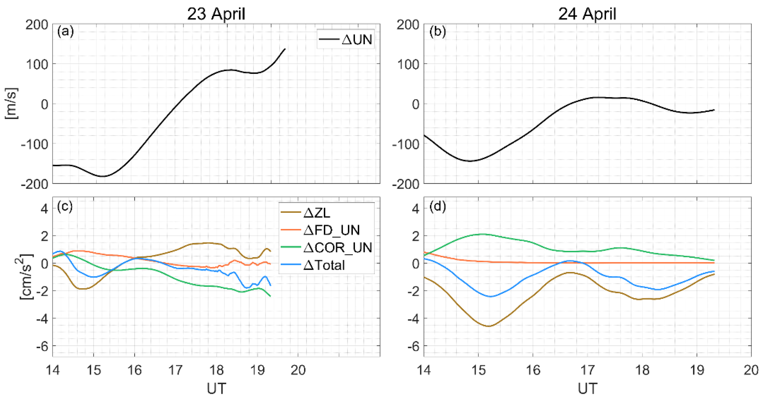
To explore the effects of the temporal variations in the IMF Bz on neutral winds, a control case with a constant Bz value of 0 nT is performed. The differences between the neutral winds in the real and control cases are the wind perturbations associated with the strong temporal oscillations of IMF Bz. Figure 8a depicts the temporal variations of zonal wind responses (ΔUN) to the temporal oscillations in the IMF Bz on 23 April. The equation about ΔUN is shown as follows: . It can be found that ΔUN is strong westward at 14–16 UT, with an average speed of 150 m/s. The peak westward ΔUN occurs at 15 UT, with a speed of 200 m/s. At the following UTs, the westward ΔUN is rapidly reduced and reverses eastward. The polarity transition is located at 17 UT. The peak of eastward ΔUN at 17–19 UT is 130 m/s at 19 UT. Maybe over 19 UT, the maximum of zonal wind changes might exist but are still unknown. An interesting phenomenon should be noted herein the enhanced ΔUN eastward gets slowed and even weakened at 18 UT. On 24 April (Figure 6b), a similar temporal variation in the ΔUN to that on 23 April is found. ΔUN is first enhanced westward from −80 m/s at 14 UT to −150 m/s at 15 UT, then eastward to 10 m/s at 17 UT, thereafter westward to −30 m/s at 18.5 UT, and finally eastward to −20 m/s at 19 UT.
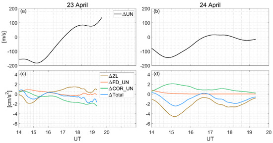
Figure 8.
The temporal variations of the UN responses (ΔUN, a,b) and the acceleration changes (c,d) during the geomagnetic storm. The left-to-right columns are for data on 23 and 24 April, respectively. ‘Total’, ‘ZL’, ‘FD_UN’, and ‘COR_UN’ are the acceleration changes due to the total force, pressure gradient, ion drag, and Coriolis, respectively. The acceleration is given in cm/s2.
Figure 8c,d provides information on the acceleration perturbations due to the total forcing, pressure gradient, ion drag, and Coriolis force on 23–24 April. The effects of other forces (i.e., centrifugal, horizontal advection, and viscosity) are relatively weaker than the above three forces. Therefore, only the acceleration responses associated with the pressure gradient (ΔZL), ion drag (ΔFD_UN), and Coriolis force (ΔCOR_UN) are displayed herein. All of those three factors are related to the collision between ions and neutrals. The plasma collisional heating is the dominant heating mechanism for the neutrals in the upper thermosphere. Therefore, the pressure gradient might be affected by the collision between ions and neutrals. The ion drag is sourced from the plasma density and the relative motion between ions and neutrals. The Coriolis force on the zonal winds is attributed to the Coriolis coefficient and the meridional winds. The meridional winds could be controlled by the pressure gradient and ion drag. Acceleration represents the ratio of speed changes. The negative (positive) acceleration changes indicate the decrease (increase) in eastward winds or the increase (decrease) in westward winds. Therefore, the temporal structures of acceleration might not be the same as those of the neutral winds.
At 14–15 UT on 23 April, the total acceleration changes are weak eastward at the beginning stage and obviously enhanced westward, with a trough of −1.5 cm/s2. The effects of the pressure gradient are westward from −0.2 cm/s2 at 14 UT to −2.0 cm/s2 at 15 UT. A comparison between the accelerations due to the total forcing and the pressure gradient shows that the pressure gradient is the primary driver. The same result can be obtained at the following UTs on 23 April. During the geomagnetic storm, the pressure gradient is related to the neutral temperature changes [20,32]. Thus, as shown in Figure 8a, the westward ΔUN at 14–15 UT might be dominated by the pressure gradient changes. However, the effects of ion drag and Coriolis force are positive, with an average acceleration of 1 and 0.2 cm/s2, respectively. The positive acceleration indicates the weakening of the westward winds. Hence, at 14–15 UT, ion drag and Coriolis force prevent the formation of ΔUN. As reported by the authors of previous studies [15,32], the ion drag is associated with two factors: one is the plasma density and the other is the relative motion between ions and neutrals. The detailed roles of plasma density and relative motion are not the focus of the present study and have thus not been included herein. Instead, we only show the complete effects of ion drag. The effects of Coriolis force on zonal winds are related to the Coriolis coefficient and meridional winds [27,42]. The Coriolis force tends to direct westward with an equatorward wind. At Mohe station, ΔVN is poleward at 14–15 UT (Figure 8a in the following section); hence, the Coriolis force effects are directly eastward, preventing the formation of ΔUN at 14–15 UT. At the phase of the enhanced ΔUN eastward (15–19 UT, Figure 6a), the acceleration changes due to the pressure gradient are strongly positive, indicating its key and positive role. The effects of ion drag are weak and perturbed at around zero, indicating its insignificant role. In comparison, the effects of Coriolis force are negative, with an average magnitude of −1.5 cm/s2. Thus, the enhanced ΔUN in eastward is also dominated by the pressure gradient, with negative contributions from ion drag and Coriolis force. On 24 April (Figure 8b,d), a similar conclusion is obtained. That is, ΔUN is controlled by the pressure gradient, with minor contributions from ion drag and negative effects from Coriolis force.
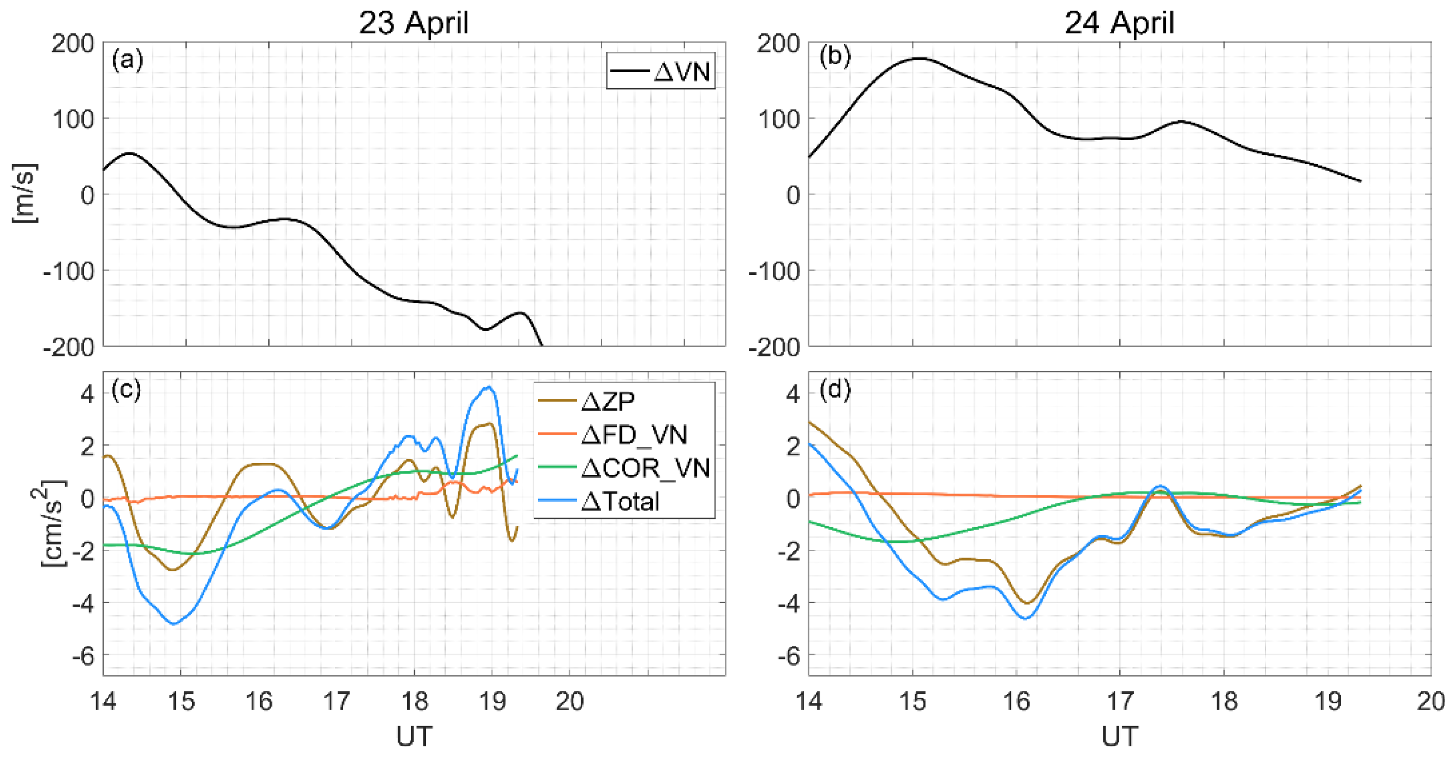
Figure 9 depicts the temporal variations in meridional wind responses (ΔVN) to the IMF Bz on 23–24 April 2023 and the associated accelerations due to different forces. The equation about ΔVN can be expressed as follows: . It can be seen that on April 23 (Figure 9a), ΔVN is generally equatorward and enhanced in equatorward. As shown in Figure 9c, the acceleration changes due to the total force, pressure gradient, ion drag, and Coriolis force are provided. The acceleration changes due to the total forcing share a large degree of similarity with that due to the pressure gradient. The acceleration changes due to ion drag are generally weak and negative, with an average magnitude close to zero. The acceleration perturbations associated with the pressure gradient are strong. They are negative at 14.5–15.5, 16.5–17.5 and 18.5 UT. The Coriolis force effects are negative at 14–17 UT, and positive at the following UTs. In summary, this equatorward ΔVN on 23 April might be related to the combined roles of pressure gradient and Coriolis force, with minor contributions from ion drag. A similar conclusion is achieved for the ΔVN on 24 April.
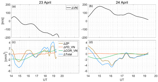
Figure 9.
Similar to Figure 6, but for the VN responses (ΔVN, a,b) and the associated accelerations (c,d). ‘Total’, ‘ZP’, ‘FD_VN’, and ‘COR_VN’ are the accelerations due to the total force, pressure gradient, ion drag, and Coriolis, respectively.
As shown in Figure 2e, the IMF Bz at 14–17 UT has an average magnitude of −7.8 nT. The southward IMF Bz occurs continually and lasts for hours. The interaction between southward Bz and the geomagnetic field can lead to the energy deposition and heat of the high-latitude neutrals. Therefore, the nighttime neutral winds at Mohe station in Figure 9c could be perturbed greatly by the pressure gradient in associated with the enhanced neutral temperature. In Figure 2e,f, the great oscillations of IMF Bz occur in the period from 18 UT on 23 April to 06 UT on 24 April. The perturbed neutral winds could have existed not only during the above periods but also at the following time (Figure 8 and Figure 9). Because the behaviors of the neutral winds are the accumulation of all forces. Furthermore, the disturbances in the neutral winds have a time delay in comparison with IMF Bz. Because the heated air needs time to travel from the high latitudes to the middle latitudes. Therefore, the nighttime neutral wind responses at Mohe station could be related to the great perturbations of IMF Bz. In Figure 2e,f, IMF Bz has a period ranging from minutes to hours. However, in Figure 8a,b and Figure 9a,b, the responses of zonal and meridional winds to IMF Bz are smooth. This is reasonable and related to large-scale traveling atmospheric disturbances (LSTADs). During storm times, the increased Joule heating at high latitudes could significantly enhance the neutral temperature, causing the upwelling of molecular-rich air. The heated air could extend to the lower latitudes through the dynamic processes, that is, LSTADs. Previous studies have demonstrated that the LSTADs have a period of 0.5–3 h [20]. Therefore, the residual zonal and meridional winds are smooth.
5. Summary
Using Swarm observed electron density and neutral density, FPI measured thermospheric winds, and TIEGCM simulations, the roles of IMF Bz on the thermospheric winds at Mohe station during the storm on 23–24 April are explored in the present work. During the study, a number of interesting results were derived as follows:
1. The meridional winds are strong/weak equatorward at pre-dawn on 23/24 April. The peak/trough of zonal winds occurs at midnight on 23/24 April.
2. The responses of zonal winds to the IMF Bz are westward and eastward at pre-midnight and pre-dawn, respectively. This finding is primarily attributed to the pressure gradient, with contributions from Coriolis force and ion drag.
3. The meridional wind perturbations are strong equatorward (–200 m/s) on 23 April. However, on 24 April, they are generally poleward and peak at midnight. This finding might be the result of the combined roles of both pressure gradient and Coriolis force.
Author Contributions
Conceptualization, K.Z. and H.W.; methodology, K.Z.; software, T.Y.; validation, Z.L. and C.Z.; data curation, K.Z.; writing—original draft preparation, K.Z.; writing—review and editing, H.W.; supervision, H.W.; project administration, H.W.; funding acquisition, H.W. and K.Z. All authors have read and agreed to the published version of the manuscript.
Funding
We are grateful for the sponsors from the National Key Research and Development Program (2022YFF0503700), the National Natural Science Foundation of China Basic Science Center (42188101), the National Nature Science Foundation of China (No. 42374200), the Fundamental Research Funds for the Central Universities (2042023kf0099), and Hubei Provincial Natural Science Foundation of China (2023AFB616). This work is also supported by the Project Supported by the Specialized Research Fund for State Key Laboratories. The authors acknowledge the use of data from the Chinese Meridian Project.
Data Availability Statement
The Swarm data can be accessed from the European Space Agency (ESA) (http://swarm-diss.eo.esa.int (accessed on 23–24 April 2023)). The FPI observations are archived from the World Data Center for Geophysics, Beijing (http://www.geophys.ac.cn/ (accessed on 23–24 April 2023)). The GNSS TEC can be obtained in madrigal (http://cedar.openmadrigal.org/ (accessed on 23–24 April 2023)). The 1 min Bx, By, Bz data are downloaded from the OMNI database available at https://omniweb.gsfc.nasa.gov/ (accessed on 23–24 April 2023). The Dst index is stored on the URL of https://wdc.kugi.kyoto-u.ac.jp/dstdir/ (accessed on 23–24 April 2023). The simulation data are available by email from Kedeng Zhang (ninghe_zkd@whu.edu.cn).
Acknowledgments
We are grateful to the Editor and anonymous reviewers for their assistance in improving the manuscript.
Conflicts of Interest
The authors declare no conflicts of interest.
References
- Rishbeth, H. The effect of winds on the ionospheric F2-peak. J. Atmos. Terr. Phys. 1967, 29, 225–238. [Google Scholar] [CrossRef]
- Blanc, M.; Richmond, A.D. The ionospheric disturbance dynamo. J. Geophys. Res. 1980, 85, 1669–1686. [Google Scholar] [CrossRef]
- Liu, J.; Wang, W.; Burns, A.; Solomon, S.C.; Zhang, S.; Zhang, Y.; Huang, C. Relative importance of horizontal and vertical transports to the formation of ionospheric storm-enhanced density and polar tongue of ionization. J. Geophys. Res. Space Phys. 2016, 121, 8121–8133. [Google Scholar] [CrossRef]
- Zhang, K.; Wang, H.; Wang, W. Equatorial nighttime thermospheric zonal wind jet response to the temporal oscillation of solar wind. J. Geophys. Res. Space Phys. 2021, 126, e2021JA029345. [Google Scholar] [CrossRef]
- Zhang, K.; Wang, H.; Liu, J.; Zheng, Z.; He, Y.; Gao, J.; Sun, L.; Zhong, Y. Dynamics of the tongue of ionizations during the geomagnetic storm on September 7, 2015. J. Geophys. Res. Space Phys. 2021, 126, e2020JA029038. [Google Scholar] [CrossRef]
- Zhang, K.; Song, H.; Wang, H.; Liu, J.; Wang, W.; Wan, X.; Wang, D.; Jin, Y. Dynamics of the tongue of ionizations during the geomagnetic storm on 7 September 2015: The altitudinal dependences. J. Geophys. Res. Space Phys. 2023, 128, e2023JA031735. [Google Scholar] [CrossRef]
- Richmond, A.D.; Ridley, E.C.; Roble, R.G. A thermosphere/ionosphere general circulation model with coupled electrodynamics. Geophys. Res. Lett. 1992, 19, 601–604. [Google Scholar] [CrossRef]
- Emmert, J.T.; Faivre, M.L.; Hernandez, G.; Jarvis, M.J.; Meriwether, J.W.; Niciejewski, R.J.; Sipler, D.P.; Tepley, C.A. Climatologies of nighttime upper thermospheric winds measured by ground-based Fabry-Perot interferometers during geomagnetically quiet conditions: 1. Local time, latitudinal, seasonal, and solar cycle dependence. J. Geophys. Res. 2006, 111, A12302. [Google Scholar] [CrossRef]
- Liu, H.; Doornbos, E.; Nakashima, J. Thermospheric wind observed by GOCE: Wind jets and seasonal variations. J. Geophys. Res. Space Phys. 2016, 121, 6901–6913. [Google Scholar] [CrossRef]
- Kondo, T.; Richmond, A.D.; Liu, H.; Lei, J.; Watanabe, S. On the formation of a fast thermospheric zonal wind at the magnetic dip equator. Geophys. Res. Lett. 2011, 38, L10101. [Google Scholar] [CrossRef]
- Miyoshi, Y.; Fujiwara, H.; Jin, H.; Shinagawa, H.; Liu, H. Numerical simulation of the equatorial wind jet in the thermosphere. J. Geophys. Res. 2012, 117, A03309. [Google Scholar] [CrossRef]
- Wu, Q.; Yuan, W.; Xu, J.; Huang, C.; Zhang, X.; Wang, J.S.; Li, T. First US-China joint ground-based Fabry-Perot interferometer observations of longitudinal variations in the thermospheric winds. J. Geophys. Res. Space Phys. 2014, 119, 5755–5763. [Google Scholar] [CrossRef]
- Zhang, K.; Wang, W.; Wang, H.; Dang, T.; Liu, J.; Wu, Q. The longitudinal variations of upper thermospheric zonal winds observed by the CHAMP satellite at low and midlatitudes. J. Geophys. Res. Space Phys. 2018, 123, 9652–9668. [Google Scholar] [CrossRef]
- Häusler, K.; Lühr, H. Nonmigrating tidal signals in the upper thermospheric zonal wind at equatorial latitudes as observed by CHAMP. Ann. Geophys. 2009, 27, L17103. [Google Scholar] [CrossRef]
- Zhang, K.; Wang, H.; Wang, W.; McInerney, J.M. Strong high-latitude zonal wind gradient observed by CHAMP and simulated by TIEGCM. J. Geophys. Res. Space Phys. 2023, 128, e2022JA030991. [Google Scholar] [CrossRef]
- Häusler, K.; Lühr, H.; Rentz, S.; Köhler, W. A statistical analysis of longitudinal dependences of upper thermospheric zonal winds at dip equator latitudes derived from CHAMP. J. Atmos. Sol. Terr. Phys. 2007, 69, L16102. [Google Scholar] [CrossRef]
- Wang, H.; Lühr, H. Longitudinal variation in zonal winds at subauroral regions: Possible mechanisms. J. Geophys. Res. Space Phys. 2016, 121, 745–763. [Google Scholar] [CrossRef]
- Wang, H.; Zhang, K. Longitudinal structure in electron density at mid-latitudes: Upward-propagating tidal effects. Earth Planets Space 2017, 69, 11. [Google Scholar] [CrossRef]
- Liu, J.; Wang, W.; Qian, L.; Lotko, W.; Burns, A.G.; Pham, K.; Lu, G.; Solomon, S.C.; Liu, L.; Wan, W.; et al. Solar flare effects in the Earth’s magnetosphere. Nat. Phys. 2021, 17, 807–812. [Google Scholar] [CrossRef]
- Zhang, K.; Liu, J.; Wang, W.; Wang, H. The effects of IMF Bz periodic oscillations on thermospheric meridional winds. J. Geophys. Res. Space Phys. 2019, 124, 5800–5815. [Google Scholar] [CrossRef]
- Zhang, K.; Wang, H.; Yamazaki, Y. Effects of subauroral polarization streams on the equatorial electrojet during the geomagnetic storm on 1 June 2013: 2. Temporal variations. J. Geophys. Res. Space Phys. 2022, 127, e2021JA030180. [Google Scholar] [CrossRef]
- Wang, H.; Lühr, H.; Ma, S.Y. The relation between subauroral polarization streams, westward ion fluxes, and zonal wind: Seasonal and hemispheric variations. J. Geophys. Res. 2012, 117, A04323. [Google Scholar] [CrossRef]
- Wang, H.; Zhang, K.D.; Wan, X.; Lühr, H. Universal time variation of high-latitude thermospheric disturbance wind in response to a substorm. J. Geophys. Res. Space Phys. 2017, 122, 4638–4653. [Google Scholar] [CrossRef]
- Dungey, J.W. Interplanetary magnetic field and the auroral zones. Phys. Rev. Lett. 1961, 6, 47–48. [Google Scholar] [CrossRef]
- Ritter, P.; Lühr, H.; Doornbos, E. Substorm-related thermospheric density and wind disturbances derived from CHAMP observations. Ann. Geophys. 2010, 28, 1207–1220. [Google Scholar] [CrossRef]
- Foster, J.C.; Vo, H.B. Average characteristics and activity dependence of the subauroral polarization stream. J. Geophys. Res. 2002, 107, SIA16-1–SIA16-10. [Google Scholar] [CrossRef]
- Zhang, K.D.; Wang, H.; Wang, W.B.; Liu, J.; Zhang, S.R.; Sheng, C. Nighttime meridional neutral wind responses to SAPS simulated by the TIEGCM: A universal time effect. Earth Planet. Phys. 2021, 5, 52–62. [Google Scholar] [CrossRef]
- Wang, H.; Zhang, K.; Zheng, Z.; Ridley, A.J. The effect of subauroral polarization streams on the mid-latitude thermospheric disturbance neutral winds: A universal time effect. In Annales Geophysicae; Copernicus Publications: Göttingen, Germany, 2018; Volume 36, pp. 509–525. [Google Scholar]
- Wang, W.; Talaat, E.R.; Burns, A.G.; Emery, B.; Hsieh, S.; Lei, J.; Xu, J. Thermosphere and ionosphere response to subauroral polarization streams (SAPS): Model simulations. J. Geophys. Res. 2012, 117, A07301. [Google Scholar] [CrossRef]
- Liu, J.; Liu, H.; Wang, W.; Burns, A.G.; Wu, Q.; Gan, Q.; Solomon, S.C.; Marsh, D.R.; Qian, L.; Lu, G.; et al. First results from the ionospheric extension of WACCM-X during the deep solar minimum year of 2008. J. Geophys. Res. Space Phys. 2018, 123, 1534–1553. [Google Scholar] [CrossRef]
- Rodríguez-Zuluaga, J.; Radicella, S.M.; Nava, B.; Amory-Mazaudier, C.; Mora-Páez, H.; Alazo-Cuartas, K. Distinct responses of the low-latitude ionosphere to CME and HSSWS: The role of the IMF Bz oscillation frequency. J. Geophys. Res. Space Phys. 2016, 121, 11528–11548. [Google Scholar] [CrossRef]
- Hsu, V.W.; Thayer, J.P.; Wang, W.; Burns, A. New insights into the complex interplay between drag forces and its thermospheric consequences. J. Geophys. Res. Space Phys. 2016, 121, 10–417. [Google Scholar] [CrossRef]
- Friis-Christensen, E.; Lühr, H.; Knudsen, D.; Haagmans, R. Swarm—An Earth observation mission investigating geo-space. Adv. Space Res. 2008, 41, 210–216. [Google Scholar] [CrossRef]
- Heelis, R.A.; Lowell, J.K.; Spiro, R.W. A model of the high-latitude ionospheric convection pattern. J. Geophys. Res. 1982, 87, 6339–6345. [Google Scholar] [CrossRef]
- Weimer, D.R. Improved ionospheric electrodynamic models and application to calculating Joule heating rates. J. Geophys. Res. 2005, 110, A05306. [Google Scholar] [CrossRef]
- Richards, P.G.; Fennelly, J.A.; Torr, D.G. EUVAC: A solar EUV flux model for aeronomic calculations. J. Geophys. Res. 1994, 99, 8981–8992. [Google Scholar] [CrossRef]
- Hagan, M.E.; Forbes, J.M. Migrating and nonmigrating diurnal tides in the middle and upper atmosphere excited by tropospheric latent heat release. J. Geophys. Res. 2002, 107, ACL 6-1–ACL 6-15. [Google Scholar] [CrossRef]
- Hagan, M.E.; Forbes, J.M. Migrating and nonmigrating semidiurnal tides in the upper atmosphere excited by tropospheric latent heat release. J. Geophys. Res. 2003, 108, 1062. [Google Scholar] [CrossRef]
- Qian, L.; Burns, A.G.; Wang, W.; Solomon, S.C.; Zhang, Y.; Hsu, V. Effects of the equatorial ionosphere anomaly on the interhemispheric circulation in the thermosphere. J. Geophys. Res. Space Phys. 2016, 121, 2522–2530. [Google Scholar] [CrossRef]
- Sori, T.; Shinbori, A.; Otsuka, Y.; Tsugawa, T.; Nishioka, M.; Yoshikawa, A. Generation mechanisms of plasma density irregularity in the equatorial ionosphere during a geomagnetic storm on December 21 and 22, 2014. J. Geophy. Res. Space Phys. 2022, 127, e2021JA030240. [Google Scholar] [CrossRef]
- Zhang, S.-R.; Coster, A.J.; Erickson, P.J.; Goncharenko, L.P.; Rideout, W.; Vierinen, J. Traveling ionospheric disturbances and ionospheric perturbations associated with solar flares in September 2017. J. Geophys. Res. Space Phys. 2019, 124, 5894–5917. [Google Scholar] [CrossRef]
- Lühr, H.; Rentz, S.; Ritter, P.; Liu, H.; Häusler, K. Average thermospheric wind patterns over the polar regions, as observed by CHAMP. Ann. Geophys. 2007, 25, 1093–1101. [Google Scholar] [CrossRef]

Disclaimer/Publisher’s Note: The statements, opinions and data contained in all publications are solely those of the individual author(s) and contributor(s) and not of MDPI and/or the editor(s). MDPI and/or the editor(s) disclaim responsibility for any injury to people or property resulting from any ideas, methods, instructions or products referred to in the content. |
© 2024 by the authors. Licensee MDPI, Basel, Switzerland. This article is an open access article distributed under the terms and conditions of the Creative Commons Attribution (CC BY) license (https://creativecommons.org/licenses/by/4.0/).