Abstract
The diurnal variation of surface incident solar radiation (Rs) has a significant impact on the Earth’s climate. Satellite-retrieved Rs datasets display good spatial and temporal continuity compared with ground-based observations and, more importantly, have higher accuracy than reanalysis datasets. Facilitated by these advantages, many scholars have evaluated satellite-retrieved Rs, especially based on monthly and annual data. However, there is a lack of evaluation on an hourly scale, which has a profound impact on sea–air interactions, climate change, agriculture, and prognostic models. This study evaluates Himawari-8 and Clouds and the Earth’s Radiant Energy System Synoptic (CERES)-retrieved hourly Rs data covering 60°S–60°N and 80°E–160°W based on ground-based observations from the Baseline Surface Radiation Network (BSRN). Hourly Rs were first standardized to remove the diurnal and seasonal cycles. Furthermore, the sensitivities of satellite-retrieved Rs products to clouds, aerosols, and land cover types were explored. It was found that Himawari-8-retrieved Rs was better than CERES-retrieved Rs at 8:00–16:00 and worse at 7:00 and 17:00. Both satellites performed better at continental sites than at island/coastal sites. The diurnal variations of statistical parameters of Himawari-8 satellite-retrieved Rs were stronger than those of CERES. Relatively larger MABs in the case of stratus and stratocumulus were exhibited for both hourly products. Smaller MAB values were found for CERES covered by deep convection and cumulus clouds and for Himawari-8 covered by deep convection and nimbostratus clouds. Larger MAB values at evergreen broadleaf forest sites and smaller MAB values at open shrubland sites were found for both products. In addition, Rs retrieved by Himawari-8 was more sensitive to AOD at 10:00–16:00, while that retrieved by CERES was more sensitive to COD at 9:00–15:00. The CERES product showed larger sensitivity to COD (at 9:00–15:00) and AOD (at 7:00–10:00) than Himawari-8. This work helps data producers know how to improve their future products and helps data users be aware of the uncertainties that exist in hourly satellite-retrieved Rs data.
1. Introduction
Surface incident solar radiation (Rs) is the primary energy source for the cycle and development of life and ecosystems on Earth [1,2,3,4]. Its existence means that the sun transmits energy outward in the form of electromagnetic waves [5]. Due to the Earth’s rotation and other atmospheric conditions, Rs appears to have significant diurnal variations, which have a profound impact on sea–air interactions, climate change, agriculture, and prognostic models [6].
Lin et al. [7] found that the diurnal variation of sea surface temperature in the East Pacific cold tongue is mainly influenced by the Rs diurnal variation. The Rs diurnal cycle also has an important impact on the diurnal variation of outer rainbands in a tropical cyclone [8]. In addition, the diurnal Rs cycle affects storm intensification and structure [9]. Pillai et al. [10] have shown that Rs diurnal variation can influence air and soil temperatures during summer and monsoon periods. Reshef et al. [11] found that prompt direct metabolic turnover in fruits is greatly affected by Rs diurnal variation. Shinod [12] used a one-dimensional mixed-layer model to study the mechanism by which the Rs diurnal cycle regulates seasonal changes in sea surface temperature in the Western Pacific Warm Pool.
Presently, various types of Rs datasets are available, including ground-based observation, reanalysis datasets, and satellite-retrieved datasets [13,14,15]. The accuracy of ground-based observation is relatively high [16]. However, due to the high maintenance cost of instruments, the distribution of stations is relatively sparse [17]. It is difficult to fully reflect the spatial characteristics of Rs. The reanalysis datasets have high spatiotemporal resolution and global coverage [18], but larger biases in cloud, aerosol, and water vapor simulations may result in poor accuracy in Rs evaluation [19,20]. Satellite-retrieved datasets have relatively high accuracy and continuity in spatial distribution, which have been proven by many evaluation studies [21,22,23]. In these works, most scholars mainly evaluated satellite-retrieved Rs data on longer time scales using monthly or annual mean data [4,15,24]. These studies also indicate that satellite-retrieved Rs has a smaller bias than reanalysis data on a long-term scale.
Instantaneous, hourly, and daily satellite-retrieved Rs data have also been widely evaluated. Tang et al. [25] incorporated high-temporal-resolution cloud products, derived from MODIS cloud products and Multifunctional Transport Satellite (MTSAT) geostationary satellite signals based on artificial neural networks (ANN) to retrieve hourly Rs. The mean bias error (bias) and root mean square error (RMSE), compared with hourly observations at three sites in the Haihe River basin of China in 2009, were 12.0 (or 3.5%) and 98.5 (or 28.9%) W m−2, respectively; their correlation coefficients (R) ranged from 0.92 to 0.93. Yu et al. [26] showed that Himawari-8-retrieved Rs had the highest accuracy compared with CERES and the other two reanalyses for instantaneous and daily values. Ma et al. [27] retrieved hourly Rs using Hamawari-8 cloud and aerosol products based on the radiative transfer model and deep neural network, and a bias of 27.6 W m−2, an RMSE of 105.4 W m−2, and an R of 0.93 were found in 2016 compared with measurements at 118 in situ radiation stations. Compared with ground radiation measurements at 33 BSRN stations in 2018, a bias of −15.4 (−8.3, −7.8) W m−2 and an RMSE of 101.0 (73.7, 32.3) W m−2 were found for instantaneous (3 h, daily) Rs from MODIS land products (MCD18) at a spatial resolution of 5 KM. The accuracy of daily MCD18 was higher than GLASS and lower than CERES [28]. A new benchmark of surface solar radiation products based on Himawari-8/AHI next-generation geostationary satellite over the East Asia–Pacific region was established by Letu et al. [29], with a much lower RMSE of 104.9 (31.5) W m−2 for hourly (daily) Rs compared with those for CERES, ERA5, and Global Land Surface Satellite (GLASS) products, providing a more accurate Rs diurnal variation for cloudy, clear, clean, and polluted conditions. Li et al. [30] applied an improved algorithm to simulate instantaneous, hourly, and daily mean Rs using cloud products from the Advanced Himawari Imager (AHI) onboard the Himawari-8 satellite. A bias of −14.1 W m−2, an RMSE of 82.4 W m−2, and an R of 0.96 for hourly Rs were shown in 2017 with reference to Baseline Surface Radiation Network (BSRN) observations. Tang et al. [31] used a more accurate hourly Himawari-8 version 3.1 (V31) aerosol optical depth (AOD) to drive a sophisticated radiative transfer algorithm to retrieve Rs, which was generally ~3 W m−2 larger than CERES-retrieved monthly Rs. In the same year, 2023, Letu et al. [32] incorporated Himawari-8/9 and Fengyun-4 and, with the aid of a radiative transfer model and machine learning techniques, developed a near-real-time monitoring system for surface solar radiation compositions. An RMSE of 19.7 W m−2 was shown for this newly developed hourly Rs data, which was much lower than the 31.5 W m−2 reported in their previous work in 2021 [29].
Bias, mean absolute bias (MAB), RMSE, and correlation coefficient (R) are widely used statistical parameters for evaluating hourly Rs data, as shown in the above studies. As Rs fluctuates with strong diurnal and seasonal variation, which can be easily retrieved by a satellite, relatively high R can be derived with these obvious unfiltered oscillations. Therefore, less sense is made of the relatively high R for direct comparisons of hourly data. For example, Rs values at noon, especially in summer, are relatively high, which directly leads to a larger bias and RMSE at this time for retrieved Rs. However, their relative bias and relative RMSE, divided by the corresponding mean state of the observed hourly Rs, may be smaller than those at sunrise and sunset.
In addition, most studies have focused on the mean state of all hourly data in a specific year and have not distinguished the difference at each hour, which hinders our understanding of the diurnal variation characterized by the hourly data. Hence, it is difficult to determine which hours are better than others for Rs retrieval. To overcome the issues mentioned above, we explored the diurnal changes in CERES for 2000.03–2021.07 by standardizing the original hourly Rs data by the top-of-atmosphere (TOA) fluxes and found that the cloud cover has more impact on the bias than aerosols in satellite-retrieved Rs [33]. However, universal insights are still lacking, as few comparisons of different satellite data have been conducted on this diurnal time scale.
Therefore, one of the motivations of this work was to comprehensively explore the diurnal Rs variations retrieved by state-of-the-art satellites spanning a relatively longer time period (not for one year), especially for high spatiotemporal Rs data. The AHI on Hamawari-8 provides better detection of cloud properties (cloud optical thickness and cloud height) and aerosols (aerosol optical thickness), which may directly promote their Rs products. Indeed, surface radiation products from Himawari-8, with the great advantages of their finer spatiotemporal resolutions of up to 0.05° (10 min)−1, have gained more attention worldwide [29,34]. To extend our previous work, which was only conducted on CERES-retrieved hourly Rs [33], this study additionally adopted the Himawari-8 hourly Rs products for comparisons. To eliminate the impact of strong diurnal and seasonal oscillations in Rs on the performance, the original hourly Rs data were all standardized by the TOA fluxes, similar to the previous work [33]. Observational data from the Baseline Surface Radiation Network (BSRN) for 2015.07–2021.07 were used as a reference. The other motivation of this work was to extensively investigate the impact of cloud types and land cover types, in addition to cloud optical depth and aerosol optical depth, on the difference between satellite-retrieved and observed hourly Rs.
Both motivations facilitated the key contributions of this paper, which are as follows: (1) This work allows a deeper investigation of Rs data retrieved from two widely used satellites and provides the extraordinary potential to reveal the cloud–radiation and aerosol–radiation interactions, even at an hourly temporal scale. (2) This work helps data producers improve their algorithm based on physical mechanisms and allows data users to learn about the uncertainties in hourly retrieved Rs data, which could be used as the input for land surface models.
The rest of the paper is structured as follows. The data and methods are described in Section 2. In Section 3, the difference between satellite-retrieved and observed Rs is shown in Section 3.1, and the related impact factors are investigated in Section 3.2. Discussion and conclusions are presented in Section 4 and Section 5, respectively.
2. Data and Methods
2.1. Ground-Based Observational Hourly Rs Data
The high-accuracy Baseline Surface Radiation Network (BSRN) was established in the early 1990s [35]. It is designed to measure multiple surface radiation fluxes. BSRN’s stations are distributed around the world, covering different climatic conditions [36], and they use well-calibrated and maintained state-of-the-art instruments. In our previous work [4], minor differences (~5 W m−2) in monthly solar radiation were found between Coupled Model Intercomparison Project (CMIP5) earth system models and BSRN, which was much smaller (~9.0–12.0 W m−2) than when using other observational networks as reference data. More than 100 Rs measurements were conducted in China. Although the instruments have improved a lot since 1993, their uncertainties are still larger than those of first-class instruments recommended by the World Meteorological Organization (WMO) [24]. Observations with lower accuracy will inevitably introduce large uncertainties in quantifying the performance of satellite retrievals; therefore, only BSRN measurements of high accuracy were used in this study despite the limited number of stations.
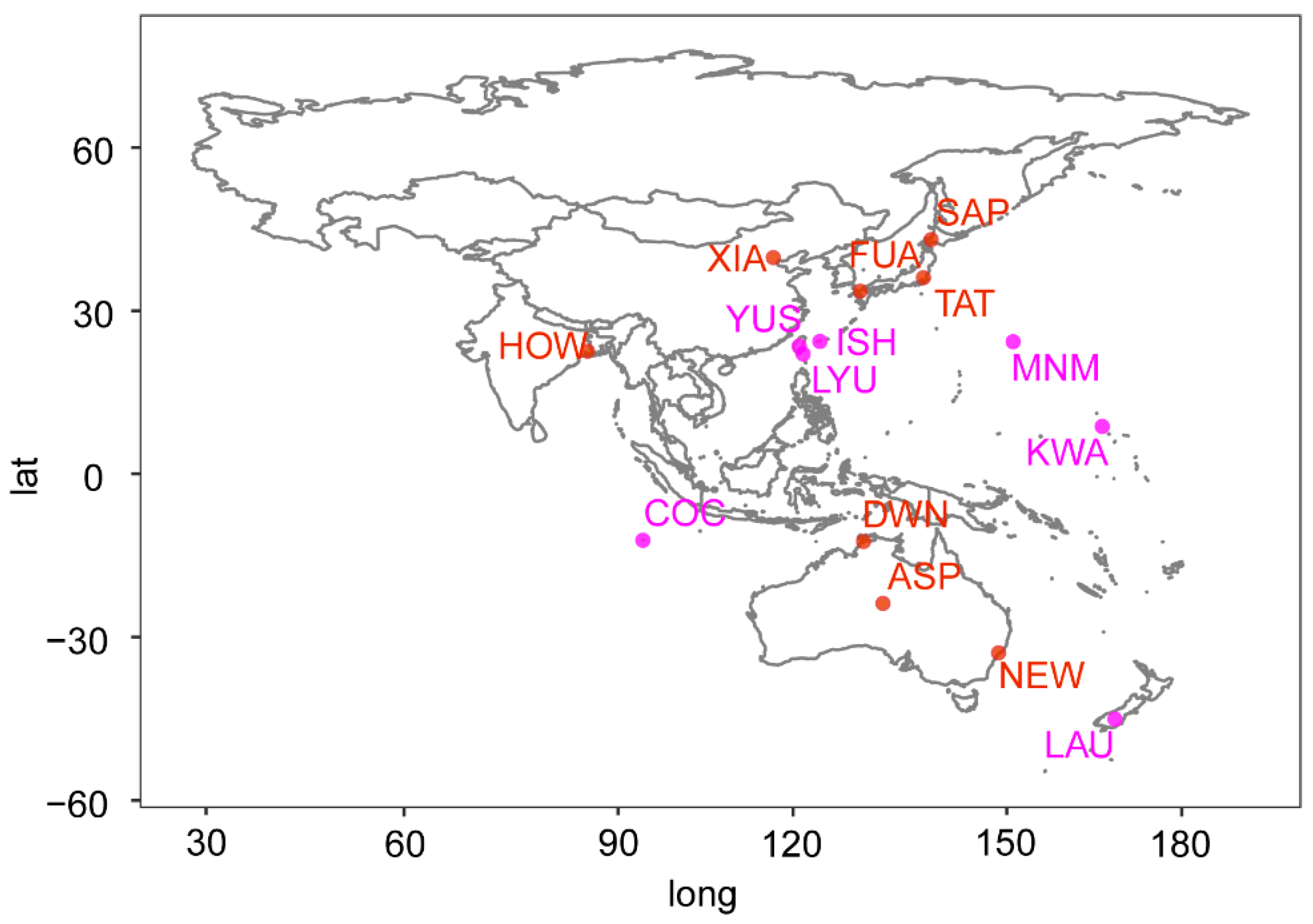
Himawari-8 monitors the spatial coverage of 60°S–60°N, 80°E–160°W, which covers a much smaller area than CERES. For a fair comparison, the East Asia–Pacific–Australia region was selected in this study. Fifteen stations are located in this area (as shown in Figure 1). Of these, eight sites, marked in red, are located on the continent, and the other seven sites, marked in magenta, are located along the island/coast.

Figure 1.
Geographical distribution of observational sites used for the evaluation of satellite-retrieved Rs data. The red and magenta circles indicate the site location on the continent and island/coast.
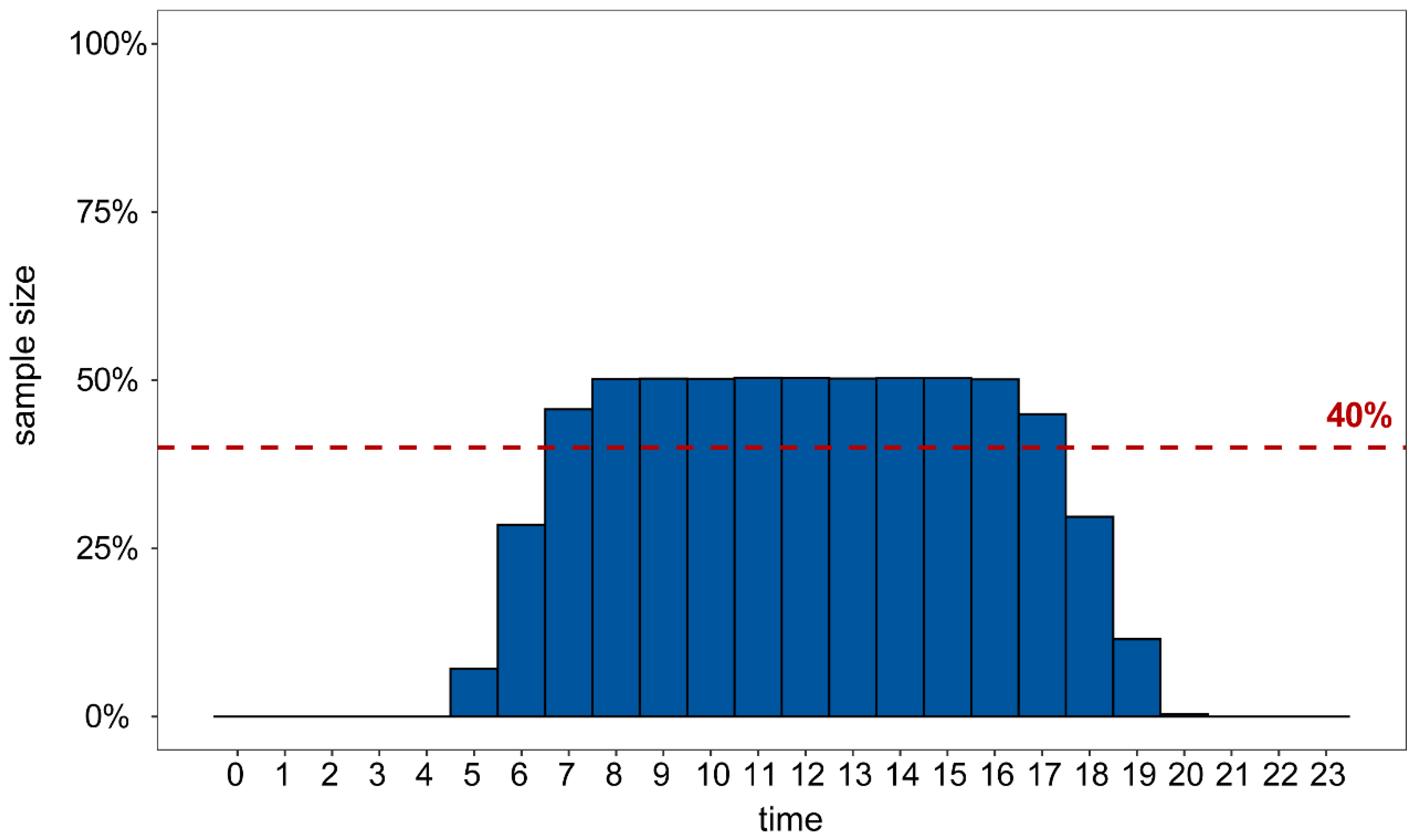
Due to infrared loss to the sky at night, the observational instrument records will be negative. This is not consistent with the actual physical situation; therefore, the nighttime measurements were discarded in this study. We solely focused on the performance of hourly Rs during the period from 7:00 to 17:00 each day, as the sample size of available data during this period was greater than 40% (see Figure 2).

Figure 2.
The sample size of the observational data at different times. The red line indicates 40% of the total sample size.
2.2. Himawari-8-Retrieved Dataset
Himawari-8, a geosynchronous meteorological satellite from the Japan Meteorological Agency (JMA), was officially launched on 7 July 2015 at 10:00 (02:00 UTC). The Himawari-8 satellite replaces MTSAT-2 (also known as Himawari-7), expanding the original 5-channel to 16-channel to include 3 visible, 3 near-infrared, and 10 infrared channels. It is located in the orbit at about 140.7°E and will observe the East Asia and Western Pacific region for 15 years. It provides Rs products with 5 km resolution (observational area of 60°S–60°N, 80°E–160°W) and 1 km resolution (observational area of 24°N–50°N, 123°E–150°E). Himawari-8, with its high temporal resolution (10 min), can better characterize cloud–radiation interactions and spatial and temporal variations of surface radiation on an hourly scale [37].
This study used hourly Short-Wave Radiation Level 3 products, hourly Aerosol Property Level 3 products, and 10 min Cloud Property Level 2 products at 5 km resolution from July 2015 to July 2021. The shortwave radiation parameterization method of the Himawari-8 Rs product is based on the work of Frouin and Murakami [38]. The algorithm utilizes the theory of plane-parallel radiation transfer. On the assumption that planetary atmospheres can be modeled as transparent atmospheres located above clouds, the effects of transparent atmospheres and clouds were treated and decoupled separately [26]. The Meteorological Research Institute (MRI) of JMA has developed an online aerosol transport model integrated with the atmospheric general circulation model (AGCM) of the Model of Aerosol Species in the Global Atmosphere (MASINGAR) [39]. Three visible bands (0.47, 0.51, and 0.64 μm) and one near-infrared band (0.86 μm) on the Himawari-8 satellite, which are sensitive to aerosol scattering and absorption, can retrieve aerosols [40]. Cloud optical depth (COD) was retrieved from thermal infrared measurements of AHI [41]. Although AHI can only detect limited regions, this new-generation geostationary meteorological satellite can offer continuous observations with a better diurnal cycle at regional scales.
2.3. CERES-Retrieved Dataset
The Clouds and the Earth’s Radiant Energy System (CERES) retrieved dataset is produced, archived, and made available to the scientific community by the Langley Research Center (LaRC), the Atmospheric Sciences Data Center (ASDC), and the National Aeronautics and Space Administration (NASA) [42]. CERES provides a global dataset with various spatial and temporal resolutions by measuring the Earth’s reflected solar and thermal radiation. Its products include TOA, surface, and atmospheric radiation. The CERES SYN1deg Ed4.1 product was used in this study.
CERES Terre and Aqua retrieved aerosol optical depth (AOD) is based on Moderate-resolution Imaging Spectroradiometer (MODIS) using the National Center for Atmospheric Research (NCAR) Model for Atmospheric Transport and Chemistry (MATCH) assimilation [43]. Cloud properties are based on imager data, which are Visible Infrared Scanner (VIRS) on TRMM and MODIS on Terra and Aqua, with plane-parallel and single-layer cloud assumptions [44]. CERES Edition 4 (Ed4) uses the revision algorithm in CERES (Ed2) [45]. Aerosol and cloud properties are the input data of the Fu and Liou [46] two-stream radiative transfer model, along with temperature and humidity profiles from the Goddard Earth Observing System (GEOS-4 and 5) Data Assimilation System reanalysis, ocean spectral surface albedo from Jin et al. [47], and broadband land surface albedo from the clear-sky TOA albedo retrieved from CERES measurements. In addition, the radiative transfer model also takes into account gaseous attenuation in the shortwave region, such as water vapor, carbon dioxide, ozone, methane, and oxygen [48].
The CERES SYN1deg Ed4.1 product contains hourly TOA fluxes, cloud properties, aerosols, and Fu–Liou radiative transferred surface and in-atmospheric (profile) fluxes. The calculated radiative fluxes are constrained by the CERES-observed TOA fluxes. We used hourly Rs, AOD, and COD with a 1° × 1° spatial resolution. For better retrieval of Rs, clouds incorporate the advantages of polar orbit and geostationary satellites. In general, sensors on polar orbit satellites have higher spectral resolutions, and those on geostationary satellites provide better detections of diurnal variation.
2.4. Methods
Rs has significant diurnal variation throughout the day due to changes in the sun’s altitude angle. Influenced by seasonal changes, it also has significant cyclical attenuation. This regular diurnal and seasonal variation could affect the calculation of relevant statistical parameters. Therefore, the standardized process was selected to remove the influence of seasonal and diurnal variation. Wild et al. [49] normalized the daily mean values with their collocated daily mean TOA fluxes rather than absolute magnitudes for trend calculation. Wang et al. [50] used the relative anomaly (%) of monthly mean-hour Rs with reference to that averaged for 1993–2014 to remove the impact of diurnal and seasonal variations on the absolute values. In this study, we followed the standardization method used in Wild et al. [49].
Standardization was carried out using the ratio of the radiation value (SW) at the time to the radiation value at the top of the atmosphere (SWTOA) at the same time, as shown in the following equation:
where SWi represents the original solar radiation at time i; SWi, std represents the standardized solar radiation at time i; and SWi, TOA represents solar radiation at TOA at time i. The following Rs indicates the standardized one.
Four parameters of bias (bias), mean absolute bias (MAB), root mean square error (RMSE), and correlation coefficient (R) were used in this study to evaluate Himawari-8 and CERES satellites, as shown in the following equation:
where Si is the satellite-retrieved Rs at hour i, and Oi is the observed Rs at hour i. The mean absolute bias was also used here to avoid the offsetting of positive and negative deviations.
3. Results
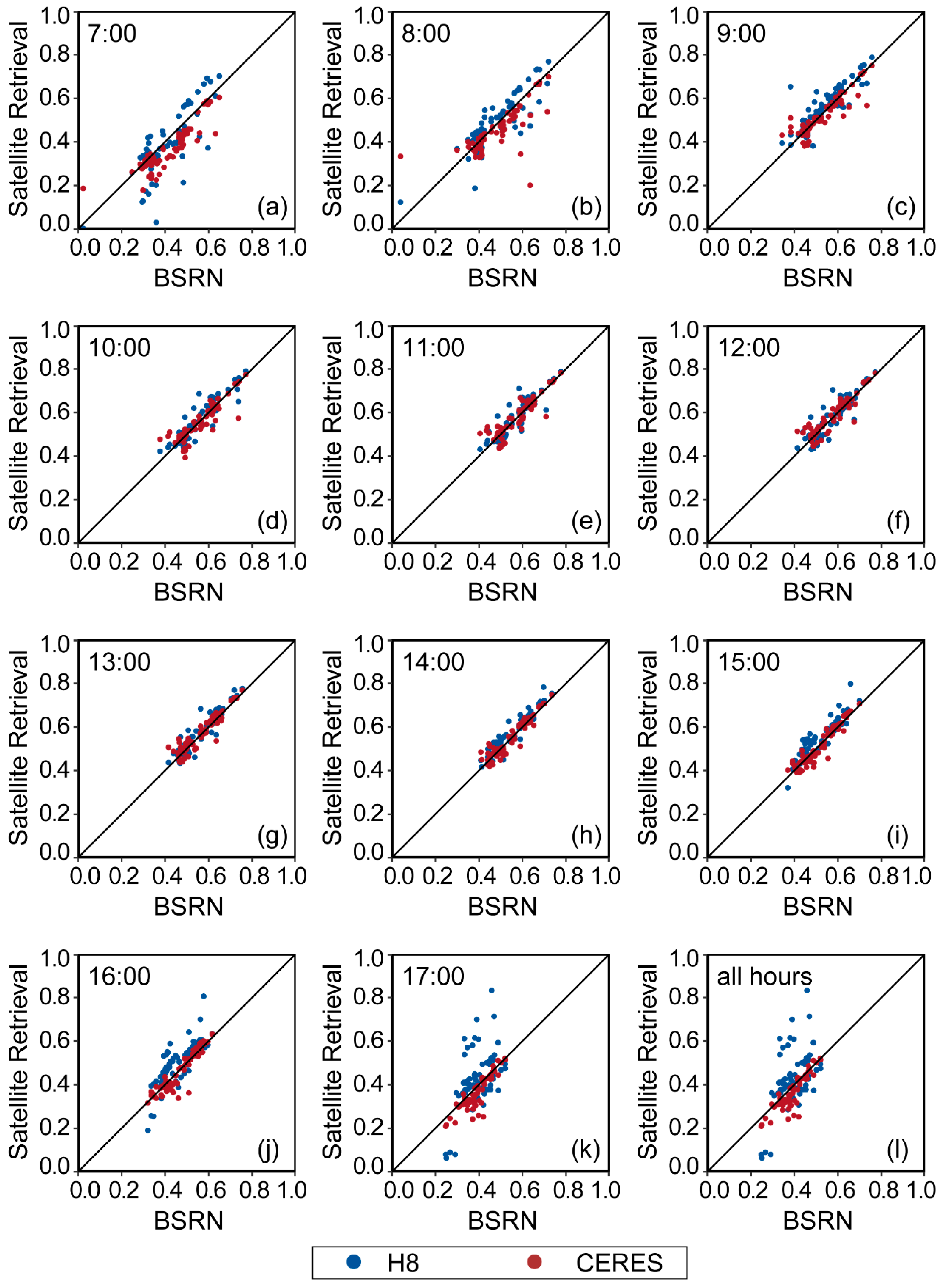
Most of the Rs values after standardization were concentrated at 0.4–0.8, except at 7:00 and 17:00, when the Rs values were in the range of 0.2–0.6, as shown in Figure 3. In this section, comparisons between satellite-retrieved and observed hourly Rs data are shown. Furthermore, the factors impacting their diurnal difference are explored.

Figure 3.
Scatter plots of the annual average of hourly satellite-retrieved and observed Rs from 2015 to 2021 at 7:00–17:00 (a–k) and all hours (l).
3.1. Difference between Satellite-Retrieved and Observed Rs
Combined with Table 1 and Figure 3, the bias of the Himawari-8 satellite was overestimated at 7:00–8:00 and 12:00–16:00, with the smallest positive bias at 12:00 (0.09%). The bias of CERES, which was less than 1% during 15:00–17:00, was overestimated; the rest of the time, the bias was negative, with the smallest negative bias at 14:00 (−0.11%). The MAB of both satellites generally decreased first and increased afterwards. For Himawari-8-retrieved Rs, the MAB ranged from 6.84% to 14.00%, with the smallest value at 11:00 and the largest value at 17:00. For hourly Rs retrieved by CERES, the MAB was the smallest at 10:00 (9.31%) and the largest at 7:00 (10.78%). The RMSE of Himawari-8-retrieved Rs was largest at 17:00 (19.28%) and smallest at 10:00 (9.72%); for CERES-retrieved Rs, it was the largest at 7:00 (13.78%) and smallest at 10:00 (12.47%). The R of the Himawari-8-retrieved Rs stabilized at 0.83–0.85 from 9:00 to 14:00, with the lowest R at 7:00 (0.63), while the R of CERES-retrieved Rs was 0.74–0.76 at 8:00–16:00.

Table 1.
Evaluation of satellite-retrieved hourly Rs against the ground-based measurements for different regions. Unit: bias %, MAB %, RMSE %.
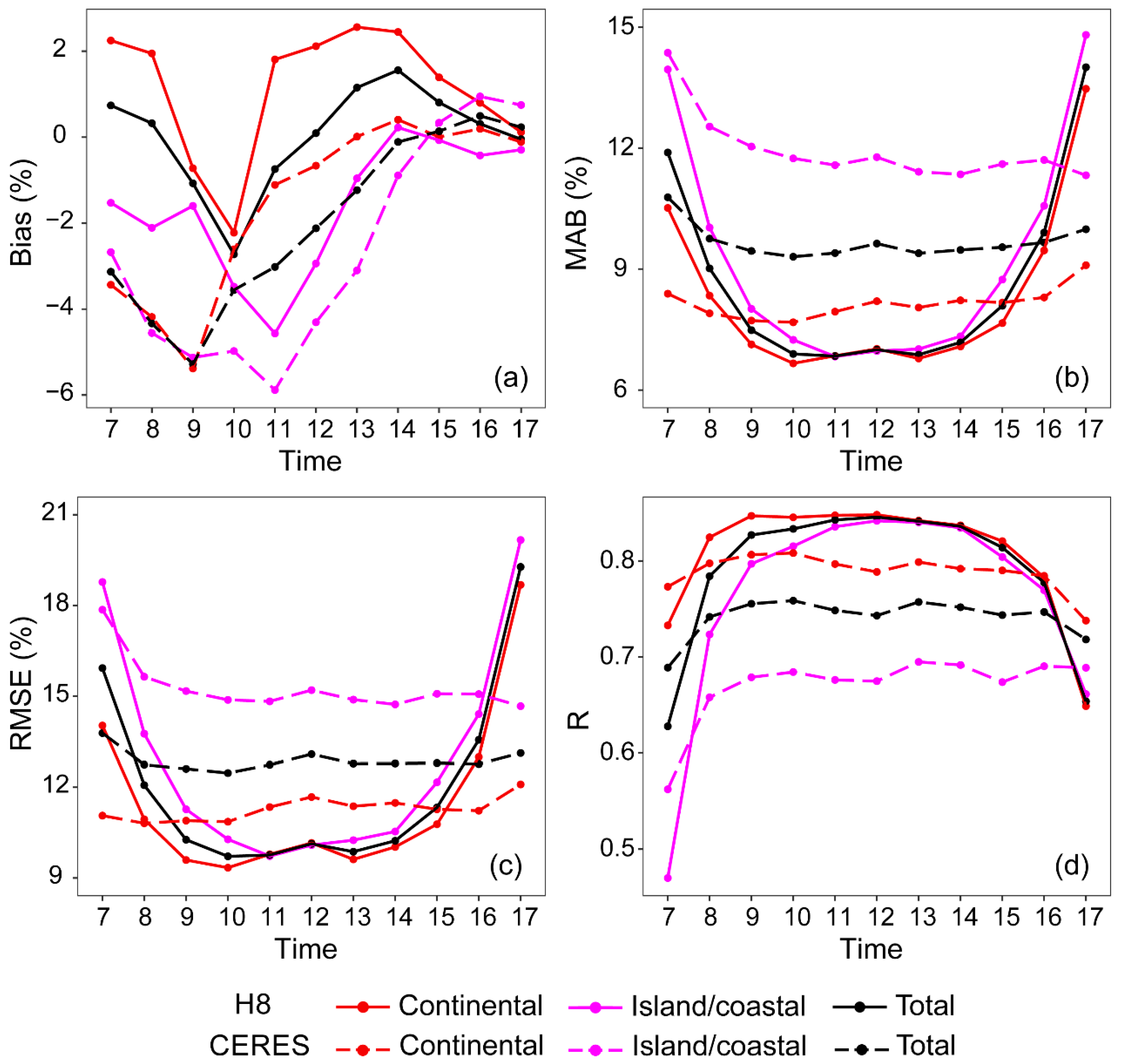
Generally speaking, the Himawari-8 satellite-retrieved Rs at 9:00–15:00 was better than that of the CERES satellite; at 7:00 and 17:00, it was worse than the CERES-retrieved Rs. Especially at 17:00, Himawari-8-retrieved Rs was the worst. Diurnal variations of statistical parameters in both satellites were similar: evaluation parameters became better and better before midday, deteriorated after midday, and were the best at midday (with the smallest MAB and RMSE). The CERES satellite-retrieved Rs was relatively stable all day except for the bias, while statistical parameters in Himawari-8 showed a large diurnal variation, which is confirmed in Figure 4.

Figure 4.
Diurnal variations of statistical parameters between hourly satellite-retrieved Rs and observed Rs for different types of sites. (a) Bias %; (b) mean absolute bias (MAB) %; (c) root mean square error (RMSE) %; and (d) correlation coefficient (R).
Figure 4 and Table 1 summarize the statistical parameters for the continental and island/coastal sites. Himawari-8-retrieved Rs at the continental sites had negative bias only at 9:00 and 10:00, while those at the island/coastal sites had negative bias except at 14:00. The mean bias at the continental sites was smaller (1.14%) than that at the island/coastal sites (−1.61%). The CERES underestimated Rs at both continental and island/coastal sites at most times, and the mean negative bias at continental sites (−1.53%) was smaller than that of island/coastal sites (−2.68%). At island/coastal sites, Himawari-8-retrieved Rs had a smaller negative bias than the CREES satellite during 7:00–13:00. At the continental sites, the absolute value of bias of the Himawari-8-retrieved Rs was smaller than that of the CERES for 7:00–10:00. However, it was opposite from 11:00 to 17:00, which may have been caused by the offset of the positive and negative bias of CERES-retrieved Rs at the continental sites.
The MAB of Himawari-8-retrieved Rs at continental sites ranged from 6.66% to 13.47%, which was overall smaller than that at island/coastal sites (6.83−14.81%). The MAB first decreased sharply at 10:00, remained stable for 11:00–13:00, and then increased after 14:00 in Himawari-8. The diurnal variation of CERES MAB was similar to that of Himawari-8, with smaller MAB at continental sites (7.68−9.10%) than at island/coastal sites (11.32−14.36%). The MAB of CERES-retrieved Rs was generally larger than that of Himawari-8 (except at continental sites at 7:00, 8:00, 16:00, and 17:00 and island/coastal sites at 17:00). Different from the Himawari-8 satellite, the MAB of the CERES-retrieved Rs at the island/coastal sites became substantially smaller with time.
The diurnal variation of RMSE was similar to that of MAB, with the Himawari-8 satellite showing a larger variation than the CERES satellite within a day. For both satellites, the RMSE at continental sites (9.34−18.68% for Himawari-8; 10.86−12.09% for CERES) was smaller than that at island/coastal sites (9.73−20.17% for Himawari-8; 14.73−17.86% for CERES). The RMSE of the Himawari-8-retrieved Rs was smaller than that of CERES for 9:00–15:00 at continental sites and for 8:00–16:00 at island/coastal sites.
For 7:00–12:00 and 14:00–16:00, the R of Himawari-8 satellite-retrieved Rs at continental sites (0.73–0.84) was larger than that at island/coastal sites (0.47–0.84), and all of them reflected the diurnal variation, in which R became higher and then lower. The R of CERES-retrieved Rs at continental sites (0.74–0.81) was significantly larger than that at island/coastal sites (0.56–0.69). The R of Himawari-8-retrieved Rs was higher than that of CERES at both continental and island/coastal stations during 8:00–15:00 (equal at 16:00 at the continental sites).
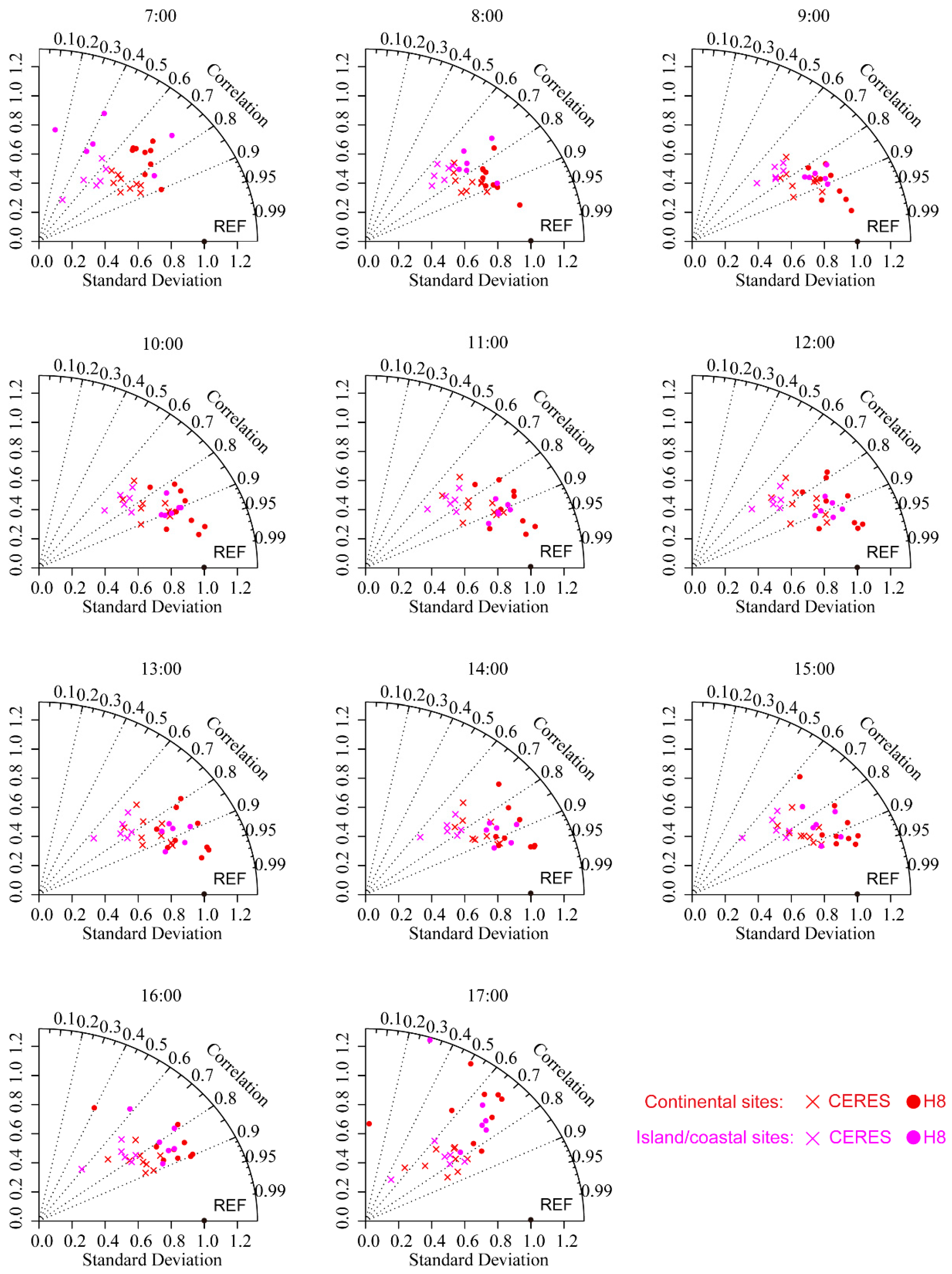
Combined with Figure 5, the satellite-retrieved Rs at continental sites was generally better than at island/coastal sites, especially for 7:00–9:00. CERES-retrieved Rs was worse at island/coastal sites than at continental sites, which may have been due to rapid weather changes and the presence of grid in land and water (edge effect) [51]. The hourly Rs retrieved by the Himawari-8 was better than that retrieved by CERES as a whole. This may be due to the higher spatial resolution of the Himawari-8 satellite. It is notable that the Himawari-8-retrieved Rs at 7:00 and 17:00 are worse than those of CERES at both continental and island/coastal sites.

Figure 5.
Taylor diagram describing the standard deviation and correlation coefficient between the hourly satellite-retrieved Rs and observed Rs at 15 selected stations. The circles and crosses denote Himawari-8-retrieved Rs and CERES-retrieved Rs. “REF” can be regarded as the point of perfection, where the value closer to the point indicates a better evaluation.
3.2. Factors Impacting the Satellite-Retrieved Rs Difference
The impact of cloud types on Rs is relatively complex. Different types of clouds have different optical properties, thickness, and spatial distribution, which in turn can have different impacts on the propagation, scattering, and absorption of Rs in the atmosphere [52,53]. According to the classification of International Satellite Cloud Climatology Project (ISCCP) cloud types, the cloud product data of Himawari-8 and CERES are divided into nine categories (see Table 2 and Figure 6).
Table 2.
Clouds are classified into different types and abbreviations based on ISCCP using cloud top pressure and cloud optical depth.

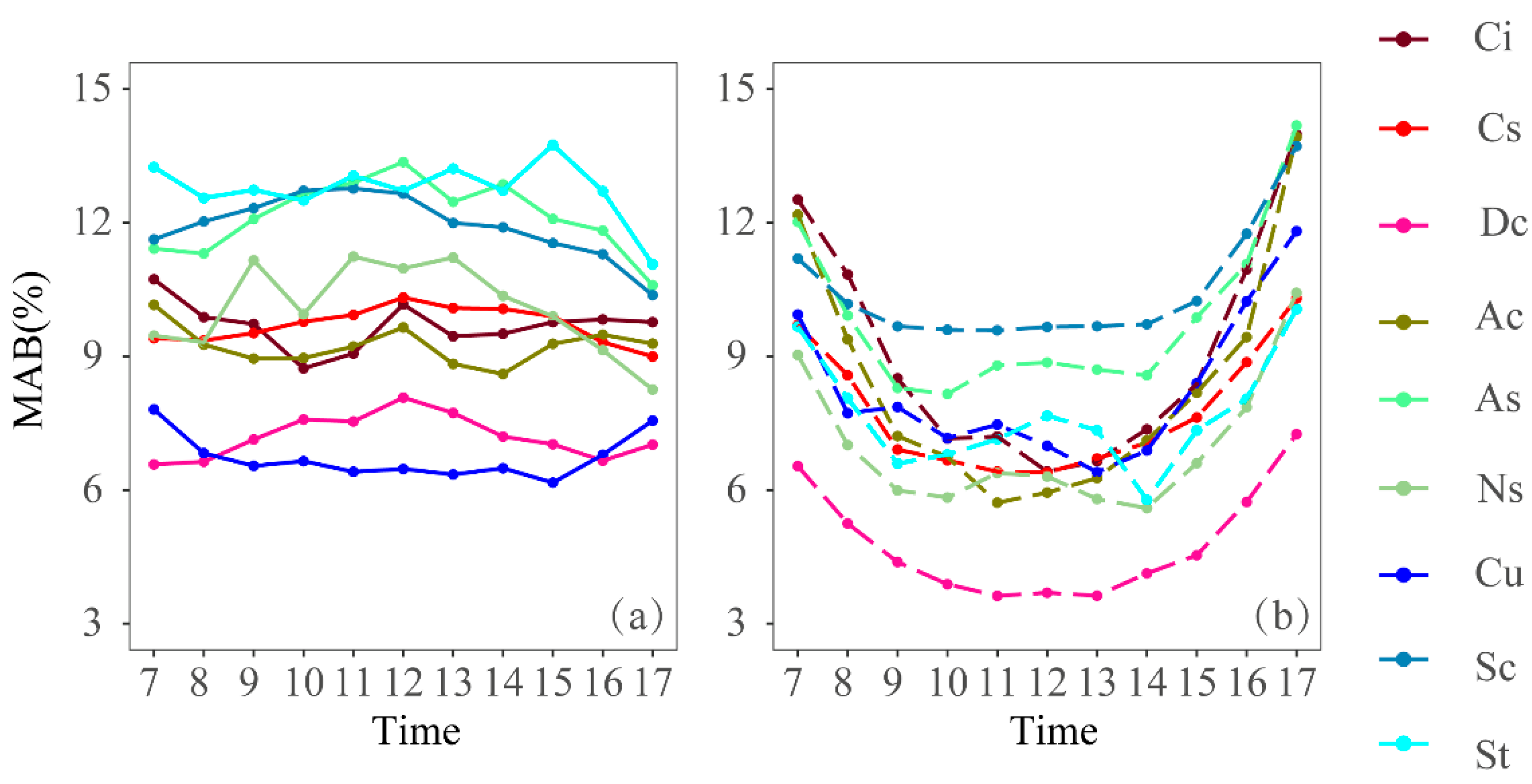
Figure 6.
MAB between satellites and BSRN hourly Rs under different cloud types from 7:00 to 17:00. (a) CERES and (b) Himawari-8.
CERES-retrieved Rs accuracy was poor in the categories of Altostratus (As), Stratocumulus (Sc), and Stratus (St). For 9:00 to 15:00, CERES-retrieved Rs had the smallest MAB under cumulus (Cu); for the remaining time, CERES-retrieved Rs had the smallest MAB under deep convection (Dc). The accuracy of Himawari-8-retrieved Rs was the highest in the deep convection (Dc) category at all hours. Stratocumulus (Sc) caused the greatest MAB of Himawari-8-retrieved Rs from 9:00 to 15:00. Cirrus (Ci), Altocumulus (Ac), Altostratus (As), and Stratocumulus (Sc) all led to poor accuracy of Himawari-8-retrieved Rs at other hours. The difference between the Rs MAB retrieved by the two satellites is relatively small during 7:00, 8:00, and 16:00. From 9:00 to 15:00, the Rs MAB retrieved by the Himawari-8 satellite was smaller than that of the CERES satellite in all cloud types except Cu. At 17:00, the performance of the Himawari-8 satellite was only superior to that of the CERES satellite in the stratus (St) category.
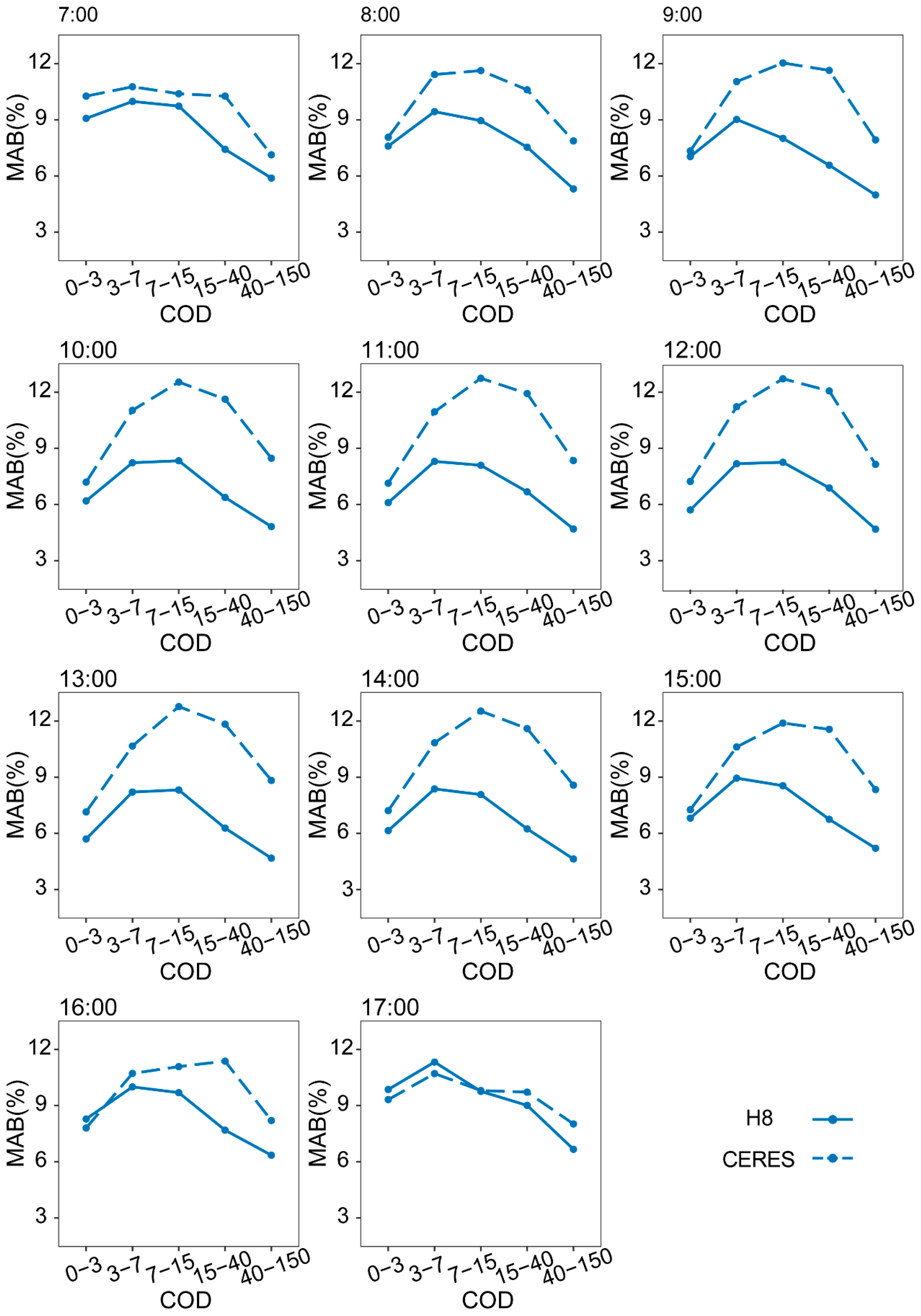
Clouds and aerosols are the key inputs for the radiative transfer model and have gained much attention in regulating satellite-retrieved Rs. Both satellites provide cloud optical depth (COD) and aerosol optical depth (AOD) products. To further explore their impacts on Rs retrieved by these two satellites, we classified COD into “0–3”, “3–7”, “7–15”, “15–40”, and “40–150” categories (see Figure 7) and AOD into “0.05–0.1”, “0.1–0.15”, “0.15–0.3”, and “0.3–8” categories (see Figure 8) to track the MAB changes among the categories.

Figure 7.
MAB between satellites and BSRN hourly Rs under different cloud optical depth (COD) categories from 7:00 to 17:00.

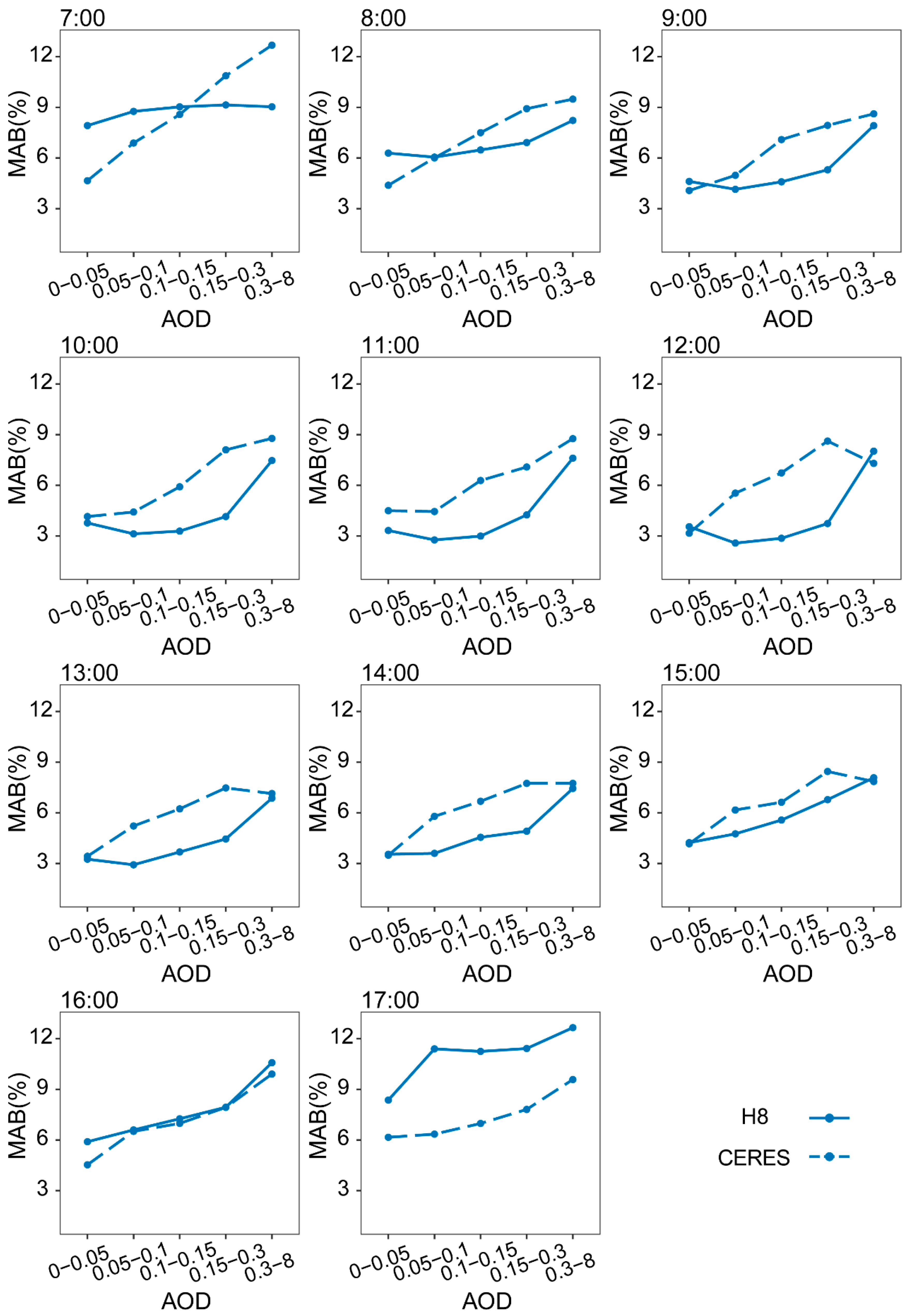
Figure 8.
MAB between satellites and BSRN hourly Rs under different aerosol optical depth (AOD) categories from 7:00 to 17:00.
For the Himawari-8 satellite, the MAB increased first and then decreased with the increase in COD. At most times, MAB reached a high in the “3–7” COD category and a low in the “40–150” category. The variation pattern of MAB from the CERES satellite was consistent with that of Himawari-8. Different from Himawari-8, the MAB had the largest value in the “7–15” category and the smallest value in the “0–3” category in the 9:00–15:00 period. At 7:00–8:00 and 17:00, both satellites had the smallest MAB in the “40–150” category. The MAB from CERES was larger than the Himawari-8 satellite except in the “0–3” category at 16:00 and in the “0–3” and “3–7” categories at 17:00. The MAB of Himawari-8 satellite-retrieved Rs increased as AOD increased, with the largest value in the “0.3–8” category. The MAB variation pattern of the CERES satellite was similar to that of the Himawari-8 satellite in most situations, except at 12:00–15:00, when the largest value appeared in the “0.15–0.3” category. It is worth noting that at 16:00, the MAB of the two satellites was almost identical. At 17:00, the MAB of the Himawari-8 satellite was completely larger than that of CERES, which is consistent with the previous conclusion. In most cases, the MAB of the CERES satellite was larger than that of the Himawari-8 satellite.
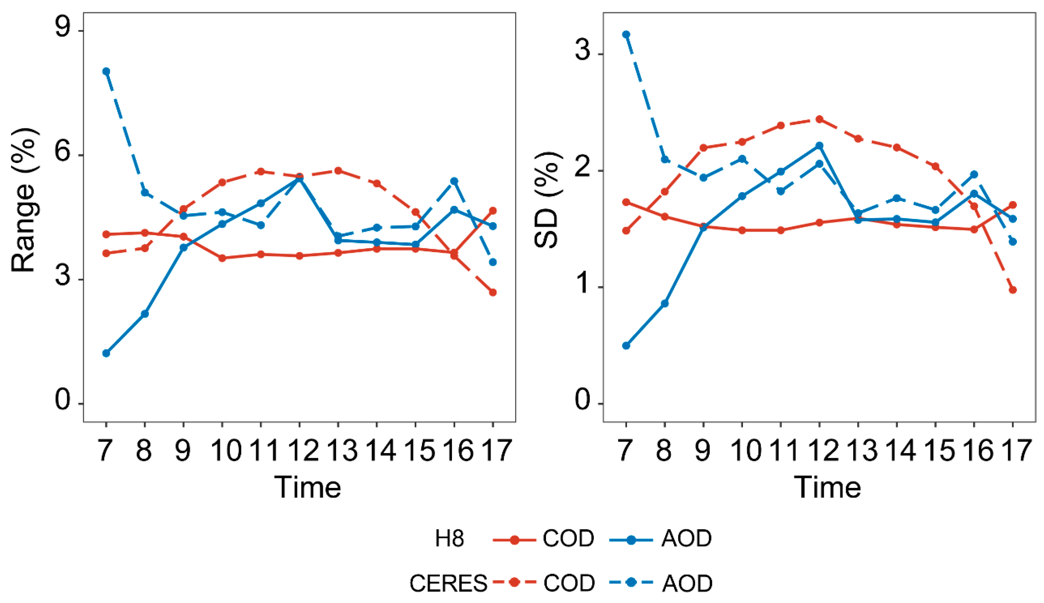
Figure 9 and Table 3 indicate the range and standard deviation of the MAB in Figure 7 and Figure 8. Results from the Himawari-8 satellite showed that it was significantly more sensitive to COD at 7:00–8:00 and 17:00. The sensitivity of COD to Himawari-8 Rs was stable through the daytime, as shown by the nearly constant values in Figure 9 (red solid line). From 9: 00 to 15: 00, the MAB of Himawari-8-retrieved hourly Rs was more sensitive to AOD (especially during 10: 00–12: 00). The MAB of CERES-retrieved Rs was more sensitive to COD during 9:00–15:00 and more sensitive to AOD at the remaining times. Comparing the two satellites, CERES was more sensitive to COD than the Himawari-8 satellite during 9:00–15:00 and more sensitive to AOD during 7:00–10:00 and 17:00. At 17:00, the Himawari-8 satellite showed higher sensitivity to both AOD and COD than CERES, which is consistent with the previous finding that Himawari-8 performed worst at 17:00. It seems that clouds play a more important role in regulating Rs during 9:00–15:00 in CERES, while aerosols impact Rs more during 10:00–16:00 in Himawari-8.

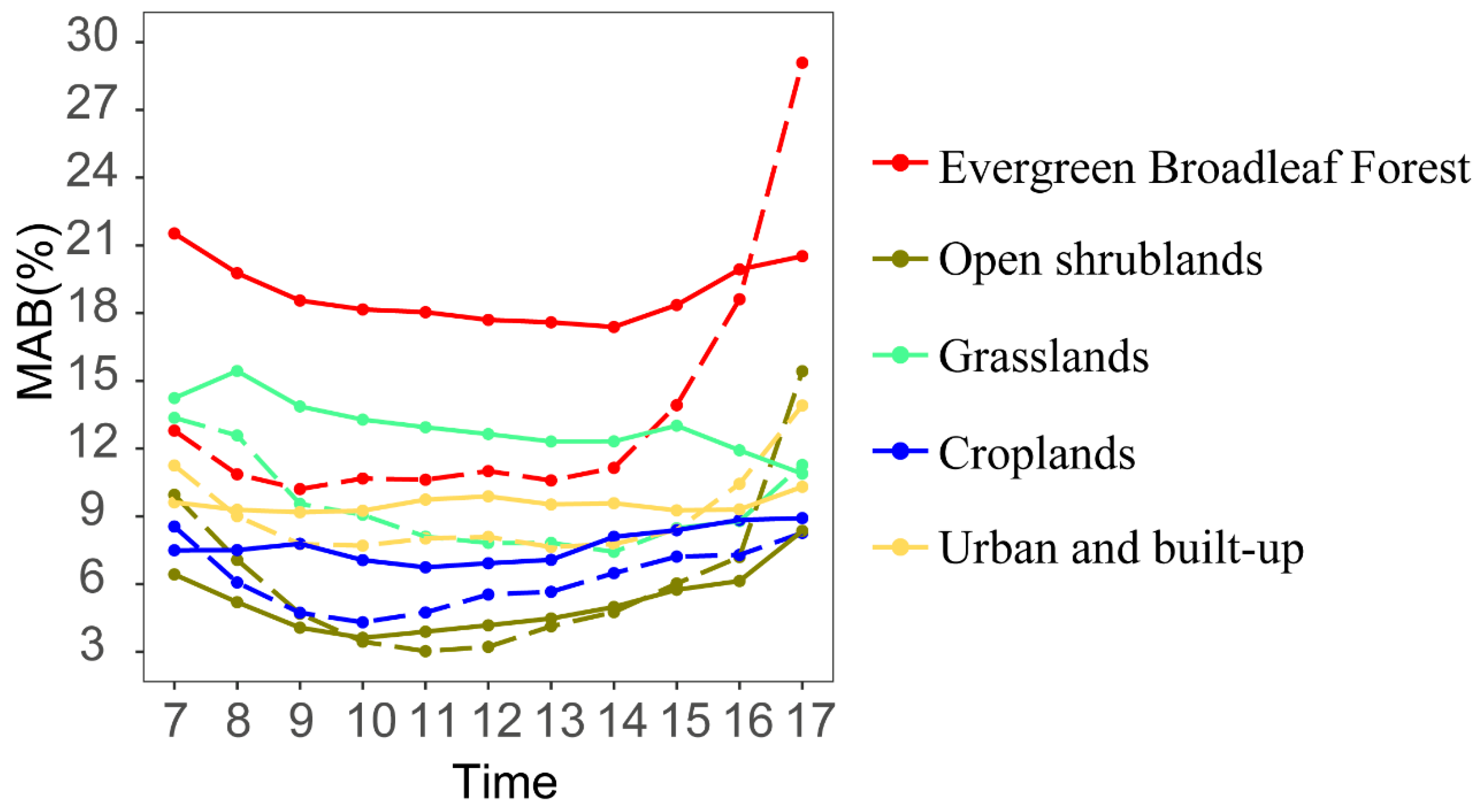
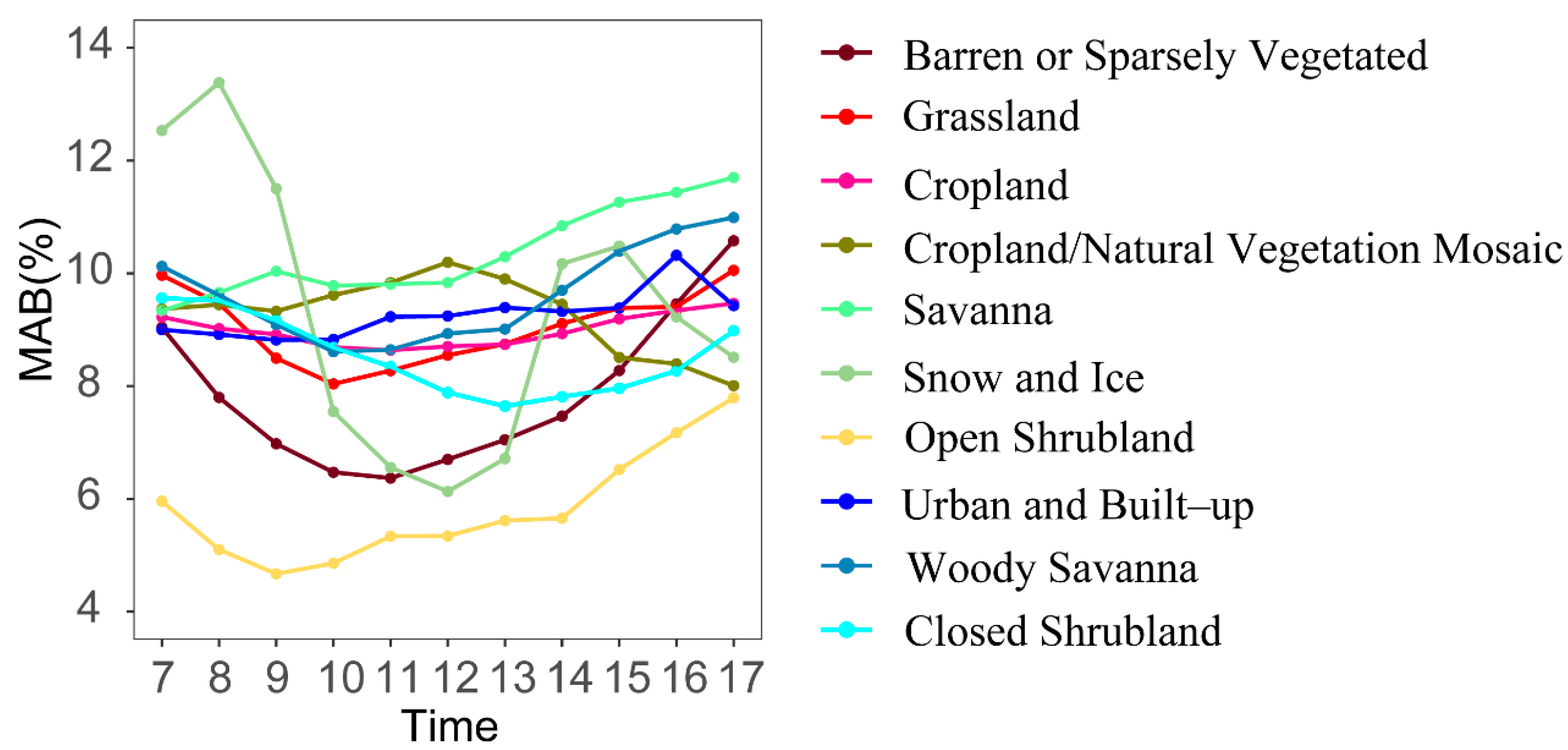
Surface energy balance, climate, ecosystem functions, and biogeochemical cycles are largely affected by land cover types [54,55,56]. Surface reflectance, influencing the multiscattering between the atmosphere and the surface, is a key input for retrieving Rs, which can be distinguished by land cover types [28]. In this study, MODIS land cover data were used to classify the sites according to the International Geosphere Biosphere Program (IGBP) land cover classification scheme. We selected nine sites from July 2015 to July 2021 for further evaluation (as shown in Table 4). Although the MAB at noon was generally lower than those at sunrise and sunset, no significant diurnal cycles in the MAB were found under different land cover types (Figure 10). During the period 9:00–14:00, the MAB of CERES-retrieved Rs under all land cover types was greater than that of the Himawari-8 satellite. Both satellite-retrieved Rs showed relatively small MAB values under open shrublands and large MAB values under evergreen broadleaf forest at most hours. It is worth noting that the MAB of Himawari-8 under evergreen broadleaf forest increased much after 14:00, especially at 17:00. The limited sites used in this study after 2015 for the East Asia–Pacific–Australia region may have led to large uncertainty in quantifying the effect of specific land cover types on Rs. The smallest MAB values were also found under open shrublands when we adopted more sites (36 sites) after 2000 over the globe to explore these effects on CERES MAB (Figure 11), which is consistent with that shown in Figure 10. Relatively large MAB values were found under grass for CERES, as shown in Figure 10 and Figure 11. A large diurnal variation of MAB was found under snow, as shown in Figure 11, which was smaller at noon and larger at sunrise and sunset. The accuracy varied significantly in shrub and forest areas (Figure 10 and Figure 11) at different times in the day, especially for Himawari-8. These failures may be partly explained by the uncertainties in surface reflectance, which is an essential determining factor in retrieving Rs, as pointed out by Wang et al. [28], and further detailed explorations are needed in future work.
Table 4.
Nine sites and their corresponding land cover types for the evaluation of satellite-retrieved hourly Rs datasets.

Figure 10.
Diurnal variations of MAB between hourly satellite-retrieved Rs and observed Rs at nine sites covered by different land cover types for 2015–2021. Solid lines for CERES and dashed lines for Himawari-8.

Figure 11.
Diurnal variations of MAB between hourly CERES-retrieved Rs and observed Rs at 39 sites covered by different land cover types for 2000–2021.
4. Discussion
This study evaluated the hourly Himawari-8 and CERES-retrieved Rs data based on observational Rs data from different global stations in the BSRN. As Rs fluctuates with the obvious diurnal and seasonal cycles, directly using the original values of hourly Rs will lead to an R value larger than 0.9, a relatively large difference at noon in summer, and a small difference at sunrise and sunset in winter. However, the diurnal variation of bias and RMSE could be opposite when using relative vias and relative RMSE. To diminish this effect, we first standardized the original hourly Rs by the TOA fluxes, which also display the strong diurnal and seasonal cycles recommended by Wild et al. [49]. Commonly used statistical parameters such as bias, RMSE, and R were used for the standardized data. MAB was also adopted as negative and positive biases at different sites, which may offset the bias calculations, especially for CERES-retrieved hourly Rs. The quality of observational data will impact the evaluation results [4]. Therefore, only BSRN sites with high accuracy were used as reference data in this study, despite their limited spatial distribution in the domain on which we are focused. Subsequently, the impacts of clouds, aerosols, and land cover types on the satellite-retrieved hourly Rs were further investigated.
The accuracy of the Himawari-8-retrieved Rs data at 8:00–16:00 was higher than that of the CERES; this may be attributed to the higher observation frequency of the Himawari-8 satellite [57]. The Himawari-8 satellite overestimates Rs data generally, while the CERES satellite tends to underestimate Rs. The results are consistent with the results of Yu et al. [26], although the R of the Himawari-8 satellite-retrieved Rs in this study was slightly lower owing to the standardization. Our study also found one point that needs to be noted: the accuracy of the Himawari-8 satellite was particularly poor at 17:00. As the time changed within the day, the accuracy of both sets of satellite-retrieved Rs data first increased and then decreased.
We divided the sites into continental and island/coastal sites for evaluation and found that the accuracy of both sets of satellite-retrieved Rs at continental sites was higher than that at island/coastal sites. This may be explained by the uncertainty in the aerosol input for retrieved Rs over island/coastal sites [58]. The spatial distribution result is consistent with other studies [30,59]. CERES satellite-retrieved Rs at island/coastal sites was even worse than that of the Himawari-8 satellite, which may be due to the higher spatial resolution of the Himawari-8 satellite and its ability to better handle edge effect issues at island/coastal sites. In addition, the diurnal variation of the statistical parameters of Himawari-8 satellite-retrieved Rs was larger than that of CERES, which was caused by the larger difference at 7:00 and 17:00 for Himawari-8.
After further studying the influencing factors of Rs, it was found that the response patterns of the two sets of data to different factors were generally consistent. The variation pattern of MAB from both satellites was roughly similar: MAB increased first with the increase in COD and then decreased, and MAB gradually increased with the increase in AOD. The variation pattern of COD-induced MAB was similar to that of our previous study on the sensitivity of CERES-retrieved Rs to cloud cover [33], both of which showed the largest MAB/bias in the middle range of COD/cloud cover. Within this range, they mainly correspond to Cirrostratus, Altostratus, and Stratocumulus. However, the variation in MAB caused by changes in COD and AOD was larger than the variation in bias caused by cloud cover and AOD, which may be due to the fact that MAB removes the effects of positive and negative offsets. CERES satellites are generally more sensitive to COD, which is consistent with other studies showing that cloud properties have greater effects on CERES than aerosols [33,58].
BSRN hourly Rs has been proven to be the highest level of observation; however, the sparse distribution over the globe is the key weakness. Although we have checked the accuracy of monthly CERES and CMIP simulations with other observational networks, including BSRN [4], much of the observational uncertainty is still unknown. Further investigation is recommended in future work, even for the hourly records. In addition, the representation of the observational sites should be further specified, although we used land cover types corresponding to the sites as a specific character to study the pattern of hourly Rs difference in this study. After that, more sites may be included for future evaluation work, which could make our conclusions more robust.
The most important thing to notice is that Hamawari-8 performed badly at sunrise and sunset hours, despite its advantageously higher spatial resolution. At most hours centered around midday, CERES-retrieved Rs was inferior to Himawari-8 Rs, especially at island/costal sites, which is mainly due to its relatively coarse spatial resolution to capture the exact surface characteristics and complex terrain. The representation of observational sites may also explain this observation. In complex topography, representativeness tends to be lower than that in homogeneous terrain. The mismatch of pixel size was ignored in this study, but it was taken into account by Letu et al. [29], who integrated grid datasets to the same spatial resolution for comparisons. Many studies have incorporated finer satellite-retrieved Rs data, e.g., the Satellite Application Facility on Climate Monitoring (CM-SAF), to explore the representation of observations on monthly, seasonal, and annual time scales over Europe and the globe and found that site-specific representativeness can be reliably estimated by the subgrid variability in a fixed grid of 1° [60,61,62]. Madhavan et al. [63] revealed that hourly Rs at a site can be representative for a few kilometers, which drives us to speculate that CERES with 1° resolution is incapable of capturing the hourly Rs at a specific site. It is inferred that the satellite-retrieved Rs diurnal variation with a spatial resolution smaller than 10 KM can be directly comparable to the site observations, and those with coarse spatial resolution are recommended to be compared with observations assembled by more than three sites in a grid cell. Further work is needed, in our opinion, to prove this speculation.
In this study, we only considered optical thickness as the main property for the effect of clouds and aerosols on Rs, which has some limitations. Cloud properties include other physical properties, such as cloud cover, cloud top height, cloud albedo, and so on. Aerosols also contain a single scattering albedo, an asymmetry factor, and other properties. In subsequent studies, other variables can be investigated to more comprehensively consider the effects of clouds, aerosols, and their interactions on satellite-retrieved Rs. In the future, more satellite-retrieved and reanalyzed hourly Rs will be further evaluated with reference to more observations of high accuracy.
5. Conclusions
This study fills the gap relating to the difference in diurnal variation of hourly Rs between CERES and Himawari-8 based on BSRN observations. Further explorations were conducted by quantifying the effects of clouds, aerosols, and land cover types on the hourly Rs for CERES and Himawari-8. The main conclusions of this study are as follows:
- The accuracy of Himawari-8-retrieved hourly Rs was higher than that of CERES for 8:00–16:00. It should be noted that the accuracy of the Himawari-8 satellite-retrieved Rs data was much poorer at 17:00.
- The Himawari-8 satellite-retrieved Rs usually showed a slight overestimation, and the CERES satellite underestimated Rs at most hours.
- The bias of the two sets of satellite-retrieved Rs data at the continental sites was smaller than that at the island/coastal sites. The bias of Himawari-8 satellite-retrieved Rs data at island/coastal stations was much smaller than that of the CERES satellite.
- Both hourly products exhibited a relatively larger MAB in the cases of Stratus and Stratocumulus. Smaller MAB values were found for CERES covered by deep convection and cumulus clouds and for Himawari-8 covered by deep convection and Nimbostratus clouds. Larger MAB values at evergreen broadleaf forest sites and smaller MAB values at open shrubland sites were found for both products.
- Himawari-8 satellite-retrieved Rs showed larger sensitivity to AOD at 10:00–16:00, while CERES was more sensitive to COD than AOD at 9:00–15:00. The changes in COD had a greater impact on MAB of CERES-retrieved Rs than Himawari-8 at 9:00–15:00, while the effect of AOD was greater on CERES than Himawari-8 hourly Rs at 7:00–10:00.
More satellite-retrieved and observed Rs data could be added in future work, which may make our evaluation results more solid. In addition, the trend of hourly Rs, an important indicator of climate change, should be taken into account as the next step of this work.
Author Contributions
Conceptualization, Q.M.; methodology, Q.M.; software, L.L. (Lu Lu); validation, L.L. (Lu Lu) and Q.M.; formal analysis, Q.M.; investigation, Q.M.; resources, L.L. (Lu Lu); data curation, L.L. (Lu Lu); writing—original draft preparation, L.L. (Lu Lu); writing—review and editing, Q.M., Y.L., and L.L. (Lingjun Liang); visualization, L.L. (Lu Lu); supervision, Q.M. All authors have read and agreed to the published version of the manuscript.
Funding
This research was funded by the National Science Foundation of China (grant number 41930970) and the BNU-FGS Global Environmental Change Program (No. 2023-GC-ZYTS-06).
Data Availability Statement
Baseline Surface Radiation Network (BSRN) data are available at https://dataportals.pangaea.de/bsrn/?q=LR0100, accessed on 19 July 2024; Clouds and the Earth’s Radiant Energy System for CERES SYN data are available at https://ceres.larc.nasa.gov/order_data.php, accessed on 19 July 2024; Himawari-8 data are available at https://www.eorc.jaxa.jp/ptree, accessed on 19 July 2024.
Acknowledgments
We thank the following institutions for sharing their data freely: the World Data Center PANGAEA for BSRN observation data, the NASA Langley Research Center Atmospheric Science Data Center for CERES SYN data, and the Japan Meteorological Agency for Himawari-8 data.
Conflicts of Interest
The authors declare no conflicts of interest.
References
- He, Y.; Wang, K. Variability in Direct and Diffuse Solar Radiation across China from 1958 to 2017. Geophys. Res. Lett. 2020, 47, e2019GL084570. [Google Scholar] [CrossRef]
- Wild, M. Global dimming and brightening: A review. J. Geophys. Res. Atmos. 2009, 114. [Google Scholar] [CrossRef]
- Wild, M.; Gilgen, H.; Roesch, A.; Ohmura, A.; Long, C.N.; Dutton, E.G.; Forgan, B.; Kallis, A.; Russak, V.; Tsvetkov, A. From Dimming to Brightening: Decadal Changes in Solar Radiation at Earth’s Surface. Science 2005, 308, 847–850. [Google Scholar] [CrossRef] [PubMed]
- Ma, Q.; Wang, K.; Wild, M. Impact of geolocations of validation data on the evaluation of surface incident shortwave radiation from Earth System Models. J. Geophys. Res. Atmos. 2015, 120, 6825–6844. [Google Scholar] [CrossRef]
- Wentz, F.J.; Schabel, M. Precise climate monitoring using complementary satellite data sets. Nature 2000, 403, 414–416. [Google Scholar] [CrossRef]
- Božnar, M.Z.; Grašič, B.; Mlakar, P.; Soares, J.; de Oliveira, A.P.; Costa, T.S. Radial frequency diagram (sunflower) for the analysis of diurnal cycle parameters: Solar energy application. Appl. Energy 2015, 154, 592–602. [Google Scholar] [CrossRef]
- Lin, P.; Liu, H.; Zhang, L. The Simulation Study of the Features of Diurnal Variation of Sea Surface Temperature in the Eastern Pacific Cold Tongue. Chin. J. Atmos. Sci. 2012, 36, 259. [Google Scholar] [CrossRef]
- Zhou, S.; Ma, Y.; Ge, X. Impacts of the diurnal cycle of solar radiation on spiral rainbands. Adv. Atmos. Sci. 2016, 33, 1085–1095. [Google Scholar] [CrossRef]
- Ge, X.; Ma, Y.; Zhou, S.; Li, T. Impacts of the diurnal cycle of radiation on tropical cyclone intensification and structure. Adv. Atmos. Sci. 2014, 31, 1377–1385. [Google Scholar] [CrossRef]
- Pillai, J.S. Diurnal Variation of Meteorological Parameters in the Land Surface Interface. Bound.-Layer Meteorol. 1998, 89, 197–209. [Google Scholar] [CrossRef]
- Reshef, N.; Fait, A.; Agam, N. Grape berry position affects the diurnal dynamics of its metabolic profile. Plant Cell Environ. 2019, 42, 1897–1912. [Google Scholar] [CrossRef] [PubMed]
- Shinoda, T.J. Impact of the Diurnal Cycle of Solar Radiation on Intraseasonal SST Variability in the Western Equatorial Pacific. J. Clim. 2005, 18, 2628–2636. [Google Scholar] [CrossRef]
- Ma, Q.; Wang, K.; He, Y.; Su, L.; Wu, Q.; Liu, H.; Zhang, Y. Homogenized century-long surface incident solar radiation over Japan. Earth Syst. Sci. Data 2022, 14, 463–477. [Google Scholar] [CrossRef]
- Feng, F.; Wang, K. Merging ground-based sunshine duration observations with satellite cloud and aerosol retrievals to produce high-resolution long-term surface solar radiation over China. Earth Syst. Sci. Data 2021, 13, 907–922. [Google Scholar] [CrossRef]
- Feng, F.; Wang, K. Determining Factors of Monthly to Decadal Variability in Surface Solar Radiation in China: Evidences From Current Reanalyses. J. Geophys. Res. Atmos. 2019, 124, 9161–9182. [Google Scholar] [CrossRef]
- Ji, Q.; Tsay, S.-C. On the dome effect of Eppley pyrgeometers and pyranometers. Geophys. Res. Lett. 2000, 27, 971–974. [Google Scholar] [CrossRef]
- Wild, M. Decadal changes in radiative fluxes at land and ocean surfaces and their relevance for global warming. WIREs Clim. Change 2016, 7, 91–107. [Google Scholar] [CrossRef]
- Urraca, R.; Huld, T.; Martinez-de-Pison, F.J.; Sanz-Garcia, A. Sources of uncertainty in annual global horizontal irradiance data. Solar Energy 2018, 170, 873–884. [Google Scholar] [CrossRef]
- Urankar, G.; Prabha, T.V.; Pandithurai, G.; Pallavi, P.; Achuthavarier, D.; Goswami, B.N. Aerosol and cloud feedbacks on surface energy balance over selected regions of the Indian subcontinent. J. Geophys. Res. Atmos. 2012, 117, D04210. [Google Scholar] [CrossRef]
- Dolinar, E.K.; Dong, X.; Xi, B.; Jiang, J.H.; Su, H. Evaluation of CMIP5 simulated clouds and TOA radiation budgets using NASA satellite observations. Clim. Dyn. 2015, 44, 2229–2247. [Google Scholar] [CrossRef]
- Pinker, R.T.; Zhang, B.; Dutton, E.G. Do Satellites Detect Trends in Surface Solar Radiation? Science 2005, 308, 850–854. [Google Scholar] [CrossRef]
- Ramirez Camargo, L.; Dorner, W. Comparison of satellite imagery based data, reanalysis data and statistical methods for mapping global solar radiation in the Lerma Valley (Salta, Argentina). Renew. Energy 2016, 99, 57–68. [Google Scholar] [CrossRef]
- Bamehr, S.; Sabetghadam, S. Estimation of global solar radiation data based on satellite-derived atmospheric parameters over the urban area of Mashhad, Iran. Environ. Sci. Pollut. Res. 2021, 28, 7167–7179. [Google Scholar] [CrossRef] [PubMed]
- Wang, K.; Ma, Q.; Li, Z.; Wang, J. Decadal variability of surface incident solar radiation over China: Observations, satellite retrievals, and reanalyses. J. Geophys. Res. Atmos. 2015, 120, 6500–6514. [Google Scholar] [CrossRef]
- Tang, W.; Qin, J.; Yang, K.; Liu, S.; Lu, N.; Niu, X. Retrieving high-resolution surface solar radiation with cloud parameters derived by combining MODIS and MTSAT data. Atmos. Chem. Phys. 2016, 16, 2543–2557. [Google Scholar] [CrossRef]
- Yu, Y.; Shi, J.; Wang, T.; Letu, H.; Yuan, P.; Zhou, W.; Hu, L. Evaluation of the Himawari-8 Shortwave Downward Radiation (SWDR) Product and its Comparison With the CERES-SYN, MERRA-2, and ERA-Interim Datasets. IEEE J. Sel. Top. Appl. Earth Obs. Remote Sens. 2019, 12, 519–532. [Google Scholar] [CrossRef]
- Ma, R.; Letu, H.; Yang, K.; Wang, T.; Shi, C.; Xu, J.; Shi, J.; Shi, C.; Chen, L. Estimation of Surface Shortwave Radiation From Himawari-8 Satellite Data Based on a Combination of Radiative Transfer and Deep Neural Network. IEEE Trans. Geosci. Remote Sens. 2020, 58, 5304–5316. [Google Scholar] [CrossRef]
- Wang, D.; Liang, S.; Zhang, Y.; Gao, X.; Brown, M.G.L.; Jia, A. A New Set of MODIS Land Products (MCD18): Downward Shortwave Radiation and Photosynthetically Active Radiation. Remote Sens. 2020, 12, 168. [Google Scholar] [CrossRef]
- Letu, H.; Nakajima, T.Y.; Wang, T.; Shang, H.; Ma, R.; Yang, K.; Baran, A.J.; Riedi, J.C.; Ishimoto, H.; Yoshida, M.; et al. A new benchmark for surface radiation products over the East Asia-Pacific region retrieved from the Himawari-8/AHI next-generation geostationary satellite. Bull. Am. Meteorol. Soc. 2021, 103, E873–E888. [Google Scholar] [CrossRef]
- Li, J.; Tang, W.; Qi, J.; Yan, Z. Mapping high-resolution surface shortwave radiation over East Asia with the new generation geostationary meteorological satellite Himawari-8. Int. J. Digit. Earth 2023, 16, 323–336. [Google Scholar] [CrossRef]
- Tang, C.; Shi, C.; Letu, H.; Ma, R.; Yoshida, M.; Kikuchi, M.; Xu, J.; Li, N.; Zhao, M.; Chen, L.; et al. Evaluation and uncertainty analysis of Himawari-8 hourly aerosol product version 3.1 and its influence on surface solar radiation before and during the COVID-19 outbreak. Sci. Total Environ. 2023, 892, 164456. [Google Scholar] [CrossRef] [PubMed]
- Letu, H.; Ma, R.; Nakajima, T.Y.; Shi, C.; Hashimoto, M.; Nagao, T.M.; Baran, A.J.; Nakajima, T.; Xu, J.; Wang, T.; et al. Surface Solar Radiation Compositions Observed from Himawari-8/9 and Fengyun-4 Series. Bull. Am. Meteorol. Soc. 2023, 104, E1772–E1789. [Google Scholar] [CrossRef]
- Lu, L.; Ma, Q. Diurnal Cycle in Surface Incident Solar Radiation Characterized by CERES Satellite Retrieval. Remote Sens. 2023, 15, 3217. [Google Scholar] [CrossRef]
- Kim, B.-Y.; Lee, K.-T. Using the Himawari-8 AHI Multi-Channel to Improve the Calculation Accuracy of Outgoing Longwave Radiation at the Top of the Atmosphere. Remote Sens. 2019, 11, 589. [Google Scholar] [CrossRef]
- Wild, M. Changes in shortwave and longwave radiative fluxes as observed at BSRN sites and simulated with CMIP5 models. AIP Conf. Proc. 2017, 1810, 090014. [Google Scholar] [CrossRef]
- Ohmura, A.; Dutton, E.G.; Forgan, B.; Fröhlich, C.; Gilgen, H.; Hegner, H.; Heimo, A.; König-Langlo, G.; McArthur, B.; Müller, G.; et al. Baseline Surface Radiation Network (BSRN/WCRP): New Precision Radiometry for Climate Research. Bull. Am. Meteorol. Soc. 1998, 79, 2115–2136. [Google Scholar] [CrossRef]
- Bessho, K.; Date, K.; Hayashi, M.; Ikeda, A.; Imai, T.; Inoue, H.; Kumagai, Y.; Miyakawa, T.; Murata, H.; Ohno, T.; et al. An Introduction to Himawari-8/9— Japan’s New-Generation Geostationary Meteorological Satellites. J. Meteorol. Soc. Jpn. Ser. II 2016, 94, 151–183. [Google Scholar] [CrossRef]
- Frouin, R.; Murakami, H. Estimating photosynthetically available radiation at the ocean surface from ADEOS-II global imager data. J. Oceanogr. 2007, 63, 493–503. [Google Scholar] [CrossRef]
- Tanaka, T.Y.; Chiba, M. Global Simulation of Dust Aerosol with a Chemical Transport Model, MASINGAR. J. Meteorol. Soc. Jpn. Ser. II 2005, 83A, 255–278. [Google Scholar] [CrossRef]
- Yumimoto, K.; Tanaka, T.Y.; Yoshida, M.; Kikuchi, M.; Nagao, T.M.; Murakami, H.; Maki, T. Assimilation and Forecasting Experiment for Heavy Siberian Wildfire Smoke in May 2016 with Himawari-8 Aerosol Optical Thickness. J. Meteorol. Soc. Jpn. Ser. II 2018, 96B, 133–149. [Google Scholar] [CrossRef]
- Wang, X.; Iwabuchi, H.; Yamashita, T. Cloud identification and property retrieval from Himawari-8 infrared measurements via a deep neural network. Remote Sens. Environ. 2022, 275, 113026. [Google Scholar] [CrossRef]
- Almorox, J.; Ovando, G.; Sayago, S.; Bocco, M. Assessment of surface solar irradiance retrieved by CERES. Int. J. Remote Sens. 2017, 38, 3669–3683. [Google Scholar] [CrossRef]
- Collins, W.D.; Rasch, P.J.; Eaton, B.E.; Khattatov, B.V.; Lamarque, J.-F.; Zender, C.S. Simulating aerosols using a chemical transport model with assimilation of satellite aerosol retrievals: Methodology for INDOEX. J. Geophys. Res. Atmos. 2001, 106, 7313–7336. [Google Scholar] [CrossRef]
- Su, W.; Charlock, T.P.; Rose, F.G. Deriving surface ultraviolet radiation from CERES surface and atmospheric radiation budget: Methodology. J. Geophys. Res. Atmos. 2005, 110. [Google Scholar] [CrossRef]
- Trepte, Q.Z.; Minnis, P.; Sun-Mack, S.; Yost, C.R.; Chen, Y.; Jin, Z.; Hong, G.; Chang, F.L.; Smith, W.L.; Bedka, K.M.; et al. Global Cloud Detection for CERES Edition 4 Using Terra and Aqua MODIS Data. IEEE Trans. Geosci. Remote Sens. 2019, 57, 9410–9449. [Google Scholar] [CrossRef]
- Fu, Q.; Liou, K.N. Parameterization of the Radiative Properties of Cirrus Clouds. J. Atmos. Sci. 1993, 50, 2008–2025. [Google Scholar] [CrossRef]
- Jin, Z.; Charlock, T.P.; Smith, W.L.; Rutledge, K. A parameterization ocean surface albedo. Geophys. Res. Lett. 2004, 31, L22301. [Google Scholar] [CrossRef]
- Kato, S.; Loeb, N.G.; Rose, F.G.; Doelling, D.R.; Rutan, D.A.; Caldwell, T.E.; Yu, L.; Weller, R.A. Surface Irradiances Consistent with CERES-Derived Top-of-Atmosphere Shortwave and Longwave Irradiances. J. Clim. 2013, 26, 2719–2740. [Google Scholar] [CrossRef]
- Wild, M.; Wacker, S.; Yang, S.; Sanchez-Lorenzo, A. Evidence for Clear-Sky Dimming and Brightening in Central Europe. Geophys. Res. Lett. 2021, 48, e2020GL092216. [Google Scholar] [CrossRef]
- Wang, Y.; Zhang, J.; Sanchez-Lorenzo, A.; Tanaka, K.; Trentmann, J.; Yuan, W.; Wild, M. Hourly Surface Observations Suggest Stronger Solar Dimming and Brightening at Sunrise and Sunset over China. Geophys. Res. Lett. 2021, 48, e2020GL091422. [Google Scholar] [CrossRef]
- Hao, D.; Asrar, G.R.; Zeng, Y.; Zhu, Q.; Wen, J.; Xiao, Q.; Chen, M. DSCOVR/EPIC-derived global hourly and daily downward shortwave and photosynthetically active radiation data at 0.1° × 0.1° resolution. Earth Syst. Sci. Data 2020, 12, 2209–2221. [Google Scholar] [CrossRef]
- Ackerman, A.S.; Toon, O.B.; Stevens, D.E.; Heymsfield, A.J.; Ramanathan, V.; Welton, E.J. Reduction of Tropical Cloudiness by Soot. Science 2000, 288, 1042–1047. [Google Scholar] [CrossRef] [PubMed]
- Stephens, G.L.; Li, J.; Wild, M.; Clayson, C.A.; Loeb, N.; Kato, S.; L‘Ecuyer, T.; Stackhouse, P.W.; Lebsock, M.; Andrews, T. An update on Earth’s energy balance in light of the latest global observations. Nat. Geosci. 2012, 5, 691–696. [Google Scholar] [CrossRef]
- Xiaoyan, Z.; Xiaoming, C.; Maosi, C.; Zhiqiang, G. Research response of land surface water and heat flux to land use land cover changes in Laizhou Bay. In Remote Sensing and Modeling of Ecosystems for Sustainability V, Proceedings of the SPIE Optical Engineering + Applications, San Diego, CA, USA, 10–14 August 2008; SPIE: Bellingham, WA, USA; p. 70830J.
- Liu, Z.; Shao, Q.; Tao, J.; Chi, W. Intra-annual variability of satellite observed surface albedo associated with typical land cover types in China. J. Geogr. Sci. 2015, 25, 35–44. [Google Scholar] [CrossRef]
- Ryu, Y.; Berry, J.A.; Baldocchi, D.D. What is global photosynthesis? History, uncertainties and opportunities. Remote Sens. Environ. 2019, 223, 95–114. [Google Scholar] [CrossRef]
- Letu, H.; Yang, K.; Nakajima, T.Y.; Ishimoto, H.; Nagao, T.M.; Riedi, J.; Baran, A.J.; Ma, R.; Wang, T.; Shang, H.; et al. High-resolution retrieval of cloud microphysical properties and surface solar radiation using Himawari-8/AHI next-generation geostationary satellite. Remote Sens. Environ. 2020, 239, 111583. [Google Scholar] [CrossRef]
- Zhang, K.; Zhao, L.; Tang, W.; Yang, K.; Wang, J. Global and Regional Evaluation of the CERES Edition-4A Surface Solar Radiation and Its Uncertainty Quantification. IEEE J. Sel. Top. Appl. Earth Obs. Remote Sens. 2022, 15, 2971–2985. [Google Scholar] [CrossRef]
- Shi, H.; Li, W.; Fan, X.; Zhang, J.; Hu, B.; Husi, L.; Shang, H.; Han, X.; Song, Z.; Zhang, Y.; et al. First assessment of surface solar irradiance derived from Himawari-8 across China. Solar Energy 2018, 174, 164–170. [Google Scholar] [CrossRef]
- Schwarz, M.; Folini, D.; Hakuba, M.Z.; Wild, M. Spatial Representativeness of Surface-Measured Variations of Downward Solar Radiation. J. Geophys. Res. Atmos. 2017, 122, 13319–13337. [Google Scholar] [CrossRef]
- Hakuba, M.Z.; Folini, D.; Sanchez-Lorenzo, A.; Wild, M. Spatial representativeness of ground-based solar radiation measurements—Extension to the full Meteosat disk. J. Geophys. Res. Atmos. 2014, 119, 11760–11771. [Google Scholar] [CrossRef]
- Hakuba, M.Z.; Folini, D.; Sanchez-Lorenzo, A.; Wild, M. Spatial representativeness of ground-based solar radiation measurements. J. Geophys. Res. Atmos. 2013, 118, 8585–8597. [Google Scholar] [CrossRef]
- Madhavan, B.L.; Deneke, H.; Witthuhn, J.; Macke, A. Multiresolution analysis of the spatiotemporal variability in global radiation observed by a dense network of 99 pyranometers. Atmos. Chem. Phys. 2017, 17, 3317–3338. [Google Scholar] [CrossRef]
Disclaimer/Publisher’s Note: The statements, opinions and data contained in all publications are solely those of the individual author(s) and contributor(s) and not of MDPI and/or the editor(s). MDPI and/or the editor(s) disclaim responsibility for any injury to people or property resulting from any ideas, methods, instructions or products referred to in the content. |
© 2024 by the authors. Licensee MDPI, Basel, Switzerland. This article is an open access article distributed under the terms and conditions of the Creative Commons Attribution (CC BY) license (https://creativecommons.org/licenses/by/4.0/).