Wet-ConViT: A Hybrid Convolutional–Transformer Model for Efficient Wetland Classification Using Satellite Data

Abstract

Accurate and efficient classification of wetlands, as one of the most valuable ecological resources, using satellite remote sensing data is essential for effective environmental monitoring and sustainable land management. Deep learning models have recently shown significant promise for identifying wetland land cover; however, they are mostly constrained in practical issues regarding efficiency while gaining high accuracy with limited training ground truth samples. To address these limitations, in this study, a novel deep learning model, namely Wet-ConViT, is designed for the precise mapping of wetlands using multi-source satellite data, combining the strengths of multispectral Sentinel-2 and SAR Sentinel-1 datasets. Both capturing local information of convolution and the long-range feature extraction capabilities of transformers are considered within the proposed architecture. Specifically, the key to Wet-ConViT’s foundation is the multi-head convolutional attention (MHCA) module that integrates convolutional operations into a transformer attention mechanism. By leveraging convolutions, MHCA optimizes the efficiency of the original transformer self-attention mechanism. This resulted in high-precision land cover classification accuracy with a minimal computational complexity compared with other state-of-the-art models, including two convolutional neural networks (CNNs), two transformers, and two hybrid CNN–transformer models. In particular, Wet-ConViT demonstrated superior performance for classifying land cover with approximately 95% overall accuracy metrics, excelling the next best model, hybrid CoAtNet, by about 2%. The results highlighted the proposed architecture’s high precision and efficiency in terms of parameters, memory usage, and processing time. Wet-ConViT could be useful for practical wetland mapping tasks, where precision and computational efficiency are paramount.

1. Introduction

Wetlands represent a critical and invaluable ecological asset situated at the intersection of land and water environments [1]. Typically experiencing periods of inundation or water saturation for a part of the year, these areas play a pivotal role in the ecosystem [2]. Within wetland regions, woodlands, shrubs, and emergent plants make up the dominant coverage [1]. Their influence on biological, ecological, and hydrological services, encompassing regional and global scales, holds profound significance. Noteworthy among these services are climate regulation, water purification, flood mitigation, and preservation of wildlife habitats [3,4,5]. Functioning as downstream recipients, wetlands receive water and waste from natural and anthropogenic sources, which is why they are known as the environment’s kidneys [6,7]. These intrinsic services and processes have collectively established wetlands as the most valuable component of nature [8].

Despite the advantages and significance of wetlands, these ecosystems have experienced considerable decline and degradation in recent decades. This process has been further exacerbated by climate change [9,10]. Wetlands are now the most endangered ecosystems due to the convergence of climate change and anthropogenic activities, characterized by shifts in land-use patterns [11]. Consequently, the implementation of effective management programs and precise monitoring techniques becomes essential in comprehensively assessing and protecting wetlands against further degradation.

The conventional method of wetland monitoring through field campaign measurements yields essential reference data for the assessment of wetlands. However, these approaches are time-consuming, demanding significant fieldwork, and are mainly applicable to localized scales [2]. Moreover, the presence of numerous wetlands in difficult-to-reach regions further emphasizes the ineffectiveness of these strategies [4]. Satellite remote sensing observations effectively address the deficiencies of traditional approaches and offer valuable insights for monitoring land-use land-cover (LULC) and wetland dynamics with frequent data collection [12,13].

Multispectral satellite sensors have gained widespread recognition and achieved significant success in the field of wetland monitoring [14,15]. Leveraging their high temporal and spatial resolution and extensive global coverage, these sensors have emerged as invaluable assets for wetland classification. However, their efficacy is constrained in specific circumstances, such as cloud cover and night-time data acquisition. Furthermore, the separation of certain wetland classes solely through the utilization of multispectral data is a challenging task [10]. The adoption of synthetic aperture radar (SAR) has expanded wetland classification due to its remarkable ability for data collection independent of solar conditions and cloud presence, along with its capacity to penetrate vegetation canopies [16] at high resolution and wide swath coverage [17]. Despite the distinct advantages offered by SAR data, the classification of wetland areas is still challenging when relying solely on SAR information. This complexity arises from the similarity in SAR backscatter response to the presence of water, a common characteristic among various wetland land covers, whether situated under the surface of vegetation canopies, at the canopy, or within the soil [18,19].

The fusion of diverse satellite data sources, such as SAR and multispectral data, facilitates the precise monitoring of various land-cover characteristics and dynamics [5,19]. The integration of multispectral and SAR data holds the potential to improve the accuracy of each individual data type. The fused data could effectively differentiate between classes exhibiting similar characteristics, such as bog and fen, surpassing the performance achieved with singular data types [20]. Previous studies have demonstrated the efficacy of this multi-sensor data fusion in mapping wetlands across diverse scales, ranging from local to large scales [21,22,23]. Large-scale wetland mapping has led to comprehensive inventories, laying the foundation for further endeavors on the development of wetland regulations, mapping of vulnerable wetland ecosystems to facilitate their preservation, and the discernment of evolving patterns within wetland environments [10].

The fusion of Sentinel-1 SAR and Sentinel-2 multispectral sensors from the Copernicus program of the European Space Agency (ESA) provides opportunities for precise LULC classification, along with facilitating wetland mapping. Both missions involve dual satellite constellations, with Sentinel-1 encompassing dual-polarized C-band SAR sensors and Sentinel-2 incorporating visible, near-infrared (NIR), and shortwave infrared bands. The Sentinel-1 SAR data provide insights into the physical and geometric structure of targets, while the Sentinel-2 multispectral data capture details regarding the molecular composition and chemical characteristics of these targets [5,24]. The fusion of these two comprehensive Sentinel datasets has gained widespread attention for the purpose of wetland mapping, exploiting their complementary features delivered at frequent revisit intervals and decent spatial resolutions [25,26].

Despite the presence of suitable datasets, such as fused SAR and multispectral imagery, the classification of wetlands remains a challenging task using remote sensing data. Each wetland class has distinctive features but shares many similarities with other wetland and non-wetland classes [27]. These similarities lead to difficulties in distinguishing between different classes, even when using spectral and backscattering information from optical and SAR imageries [28]. The application of nonparametric machine learning (ML) methodologies has addressed this issue to a feasible extent. ML algorithms, such as decision tree [29], random forest [30,31], and support vector machines [32,33], have shown great potential for wetland classification. For example, the fusion of Sentinel-1 and Sentinel-2 data to produce successive generations of Canadian wetland inventory maps is an example of recent development using the twin Sentinel mission [34,35]. They utilized random forest classification techniques and yielded comprehensive insights into the spatial extent, condition, and distribution of wetlands across Canada. Nevertheless, the capability of ML techniques remains circumscribed by the procedure of feature selection. Consequently, rigorous feature selection has a vital role in the context of ML classification techniques [5,36], yet this could sometimes be a challenging and tedious process that requires significant domain expertise.

Deep learning (DL) models have emerged as efficient tools for automatically extracting optimal features, addressing the challenge of feature selection in ML methods [37,38]. In the field of remote sensing, DL techniques have achieved considerable success across various applications, including LULC as well as wetland classification. A range of DL methods, such as feed-forward multilayer perceptron (MLP), convolutional neural network (CNN), recurrent neural network (RNN), graph neural network, generative adversarial network (GAN), and the more recent transformer-based models, have been used for wetland mapping. Using their kernel abilities to extract neighboring pixel information, CNN models have particularly demonstrated efficacy in image classification tasks. DeLancey et al. [39] presented the superior performance of CNNs when compared to conventional ML and shallow learning approaches in the classification of Alberta wetlands. Yang et al. [40] compared twelve well-known CNN architectures in the classification of urban wetlands within Shenzhen, China, using Sentinel-2 multispectral data. This analysis revealed the superior performance of the DenseNet121 architecture compared to the other well-known CNN models.

Recent studies suggested that the development of hybrid DL architectures has the potential to use the strengths of each model, which could result in improved accuracies. Jafarzadeh et al. [41] proposed a multimodal DL model comprising a shallow CNN and a graph convolutional network for wetland classification. Through the fusion of Sentinel-1 and Sentinel-2 data, their proposed model indicated superior performance in comparison to traditional ML and CNN models. Their hybrid model results showed significant promise for large-scale wetland mapping while requiring only a minimal amount of training data. Hosseiny et al. [5] presented a spatial–temporal ensemble DL model, WetNet, which included three distinct submodels of RNNs and CNNs. The model’s performance was assessed within a wetland area in Newfoundland, Canada, where it surpassed the capabilities of state-of-the-art CNN and RNN models.

CNN model capabilities are limited when capturing long-range spatial dependencies within satellite remote sensing images due to their inherent focus on local features. Transformer architectures, on the other hand, have recently shown great promise in their ability to overcome this restriction by using self-attention mechanisms [42,43,44]. With the recent advancements of transformer-based models in natural language processing (NLP), these models have paved their way into the field of wetland classification. Transformer models benefit from generalization capabilities to extract long-range patterns [1,7]. Several studies demonstrated the adaptability of transformer-based models to wetland classification. For example, Jamali et al. [1] trained a GAN model to generate synthetic data and subsequently classified them using a vision transformer (ViT) model to map wetlands across three study areas in New Brunswick, Canada. In another investigation by Jamali and Mahdianpari [7], the application of the shifted windows transformer (Swin) model for coastal wetland classification, using the integration of Sentinel-1 and Sentinel-2 data, yielded remarkable outcomes. In comparison to traditional CNN models, the Swin transformer model resulted in more than 14% improvement in classification accuracy.

Despite the notable potential of transformer models in capturing long-range information, they have limited capabilities in handling neighboring information of remote sensing images. However, by combining transformer and CNN architectures, it is possible to address this shortcoming and harness the potential of both models effectively. As a result, combining the advantages of CNNs and transformers offers the chance to improve the classification accuracy of both individual designs even further. Qi et al. [45] demonstrated the effectiveness of integrating global and local information in hyperspectral image classification using a hybrid convolutional transformer model, where 3D convolutions are embedded into a spatial–spectral dual-branch transformer model. This hybrid approach also led to significant improvements in classification accuracy, underscoring the potential benefits of hybrid CNN–transformer models in other remote sensing applications. Jamali et al. [19] introduced the WetMapFormer classifier in this context, which combines CNN and transformer models. This approach involves the utilization of CNNs in initial blocks, followed by a local window attention transformer block. This hybrid model resulted in a higher accuracy for mapping wetland classes, surpassing the performance of well-known CNN and transformer models.

Despite these advancements, existing models have notable deficiencies. CNNs, while effective in capturing local features, struggle with long-range spatial dependencies crucial for accurate wetland classification. Transformers, although adept at capturing long-range dependencies, suffer from high computational costs and complexity, particularly when dealing with large spatial dimensions. Furthermore, there are limited studies exploring hybrid models that combine the strengths of both CNNs and transformers to achieve higher accuracies with lower computational costs. For example, the WetMapFormer classifier introduced by Jamali et al. [19] demonstrated the potential of hybrid architectures by integrating CNN and transformer models, achieving superior classification accuracy. WetMapFormer achieves this with a significantly lower number of parameters and reduced computational cost compared to traditional CNN or transformer models. This efficiency makes it particularly suitable for large-scale wetland mapping, where computational resources are often a limiting factor. However, the exploration of such hybrid models remains sparse. The advantageous design of a hybrid architecture specifically for wetland classification arises from the unique characteristics of wetlands, which require both local detail and long-range spatial dependencies for accurate classification. Wetlands exhibit complex patterns that are influenced by various environmental factors and surrounding land cover types. Developing a hybrid architecture specifically designated for wetland mapping could be beneficial in achieving even higher accuracy at a reasonable computational cost.

A main challenge in using transformer models for wetland classification is their high computational complexity and requirement for a substantial amount of training samples. Particularly, the computational complexity of transformer models increases quadratically in relation to spatial dimensions [46]. Therefore, considering their possible high cost, using transformer models for practical mapping cases could be challenging and infeasible. This study mitigates the computational cost of transformers by introducing a novel hybrid CNN–transformer model, namely Wet-ConViT, designed for precise wetland classification with optimal computational complexity. Levering Sentinel-1 and Sentinel-2 data sources, the hybrid Wet-ConViT model consists of a sequence of convolutional and transformer blocks. By using multi-head convolutional attention rather than self-attention, these blocks considerably reduce the computational complexity of vanilla ViT models. Furthermore, the model uses a local feed-forward network (LFFN) that incorporates local CNN-based insights into the feed-forward stage of transformer architectures. This cohesive fusion of convolutional and transformer components not only overcomes computational challenges but also improves the model’s capacity to accurately classify wetlands using remote sensing imagery data.

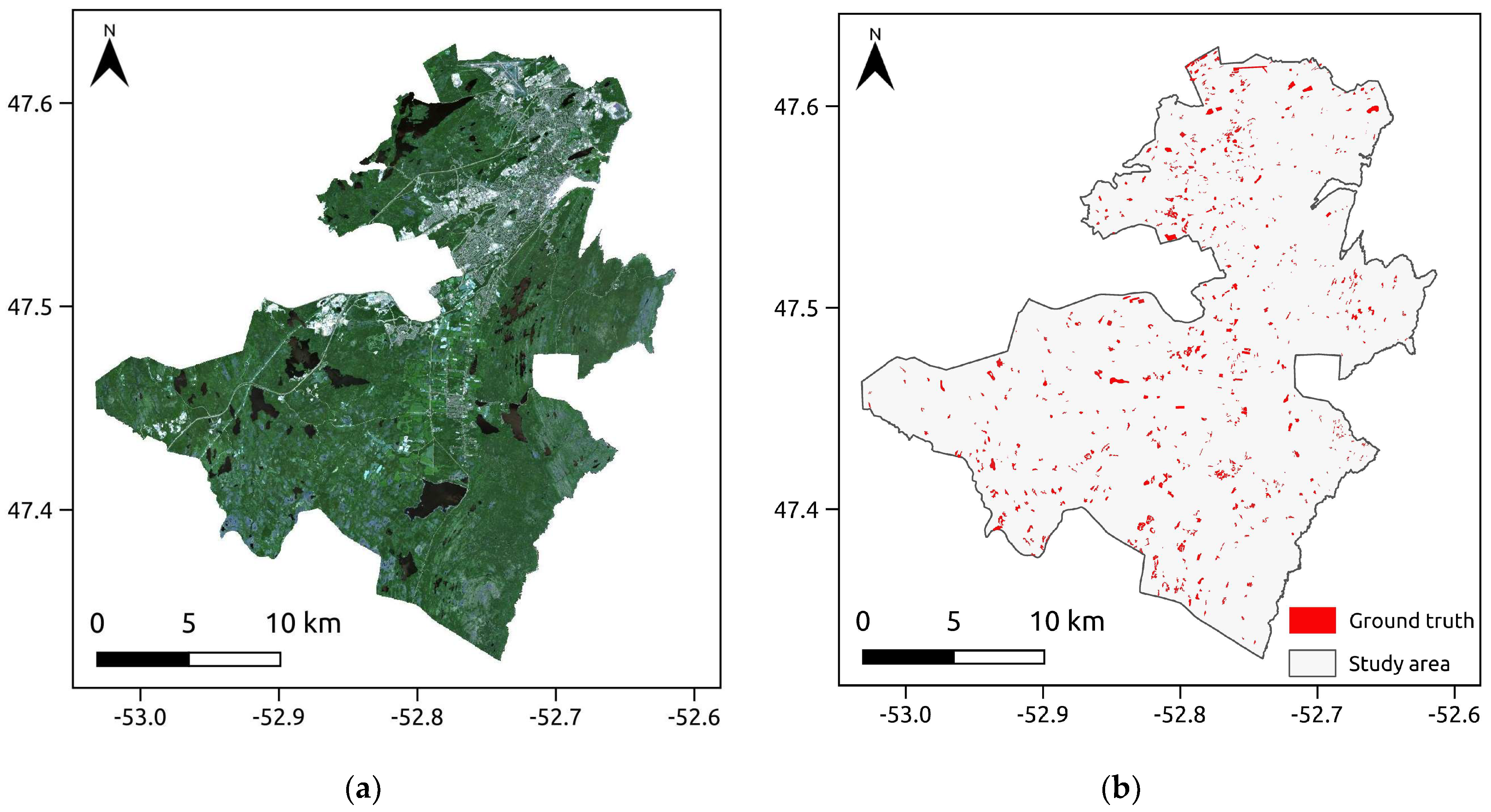
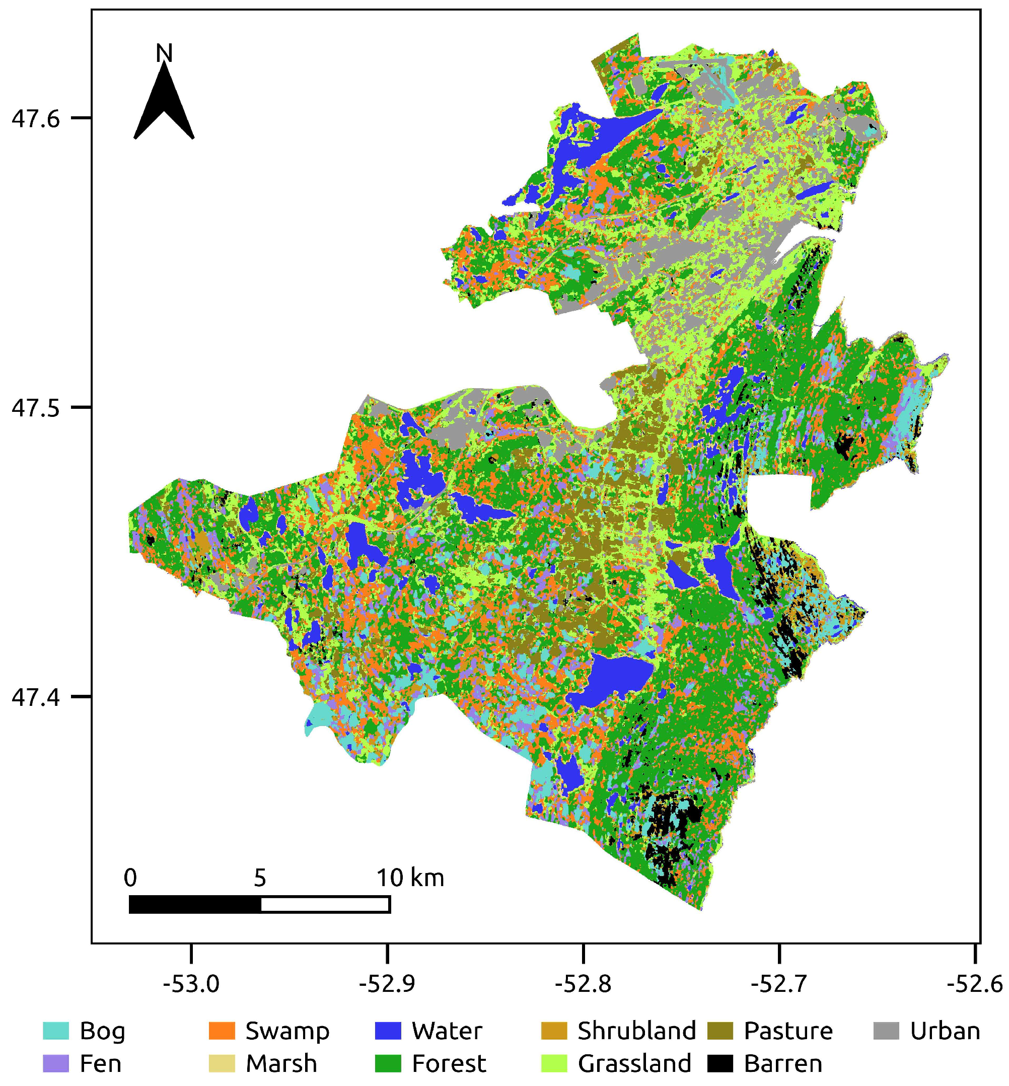
2. Study Area and Dataset

The study area under investigation is St. John’s, located on the Avalon Peninsula in the southeastern region of Newfoundland Island, Canada. This island has a humid continental climate, significantly influenced by the nearby Atlantic Ocean. The majority of land cover type in Newfoundland is wetlands, encompassing various wetland categories such as bogs, fens, marshes, swamps, and water bodies. Other land cover types, such as forests, shrublands, pastures, barren, and urban areas, are also considered in this study.

Reference Data

To gather accurate annotated ground truth data, a methodology similar to previous studies was employed [47,48,49,50]. Previous classifications and wetland ground-truth data from 2015 to 2019 were reviewed to identify additional wetlands for field verification, ensuring a distributed and representative sample within the study area. The field campaign involved visiting wetlands identified through prior classifications and remote sensing data to ensure a distributed and representative sample within the study area.

During the campaign, wetlands were classified according to the Canadian Wetland Classification System [51]. Additionally, the fieldwork included collecting Global Positioning System (GPS) data, photographs, and field notes to determine the land cover types. Due to accessibility and time constraints, only wetlands within 200 m of roads and pathways were surveyed. These wetlands were later determined using very high-resolution (VHR) imagery, LiDAR-derived digital elevation models (DEMs), and ancillary field data.

To verify data accuracy, the collected polygons were cross-validated against multi-seasonal VHR imagery and previous datasets collected in prior years. Remote sensing-based vegetation indices, such as the normalized difference vegetation index (NDVI), were used to verify vegetation patterns and validate classifications. Additionally, non-wetland land cover information was integrated using VHR imagery, Google Earth multi-seasonal imagery, and the Agriculture and Agri-food Canada’s 2018 Crop Inventory map [52], resulting in a comprehensive dataset of both wetland and non-wetland classes.

The annotated dataset is shown in Figure 1 and detailed in

Table 1. Number of ground truth land cover polygons and samples per class.

Class	Polygons	Samples
Bog	98	42,148
Fen	113	29,648
Swamp	116	15,424
Marsh	49	3445
Water	68	24,615
Forests	103	35,452
Shrublands	37	6400
Grassland	126	17,624
Pastures	47	19,745
Barren	24	1789
Urban	48	25,308
Total	829	221,598

. It includes 829 classified polygons and 221,598 sample pixels. Of these, 115,280 samples represent wetland classes, while 106,318 samples represent non-wetland classes. Among the wetland samples, bog and fen were the most common categories, accounting for more than 30% of all samples.

It is evident from Table 1 that there is a high class imbalance between the different land cover classes. For example, in our dataset, the bog and fen classes have significantly more samples (42,148 and 29,648, respectively) compared to classes like marsh and barren (3445 and 1789, respectively). Class imbalance can potentially affect the training and testing phases of machine learning models by biasing the model towards the majority classes. The proposed Wet-ConViT model and other compared models are inherently robust to class imbalances due to their complex architectures, which are capable of learning from limited samples. The use of convolutional and transformer blocks helps capture both local and global patterns, improving the model’s ability to generalize across classes with fewer samples. Despite the imbalance, the results indicate that the proposed model achieved high accuracy in classifying various wetland classes, demonstrating its effectiveness even in the presence of class imbalance.

Sentinel-1 SAR and Sentinel-2 multispectral time series data from the summer of 2021 were obtained through the Google Earth Engine (GEE) cloud platform. The acquired Sentinel-1 dataset comprises ground range-detected (GRD) dual-polarized VV and VH data acquired from the ascending orbit, as well as dual-polarized HH and HV data from the descending orbit at a spatial resolution of 10 m. All four collected SAR backscatter layers are the average composite of the summer time series, which reduces the speckle noise level of the backscatter layers. Sentinel-1 data are collected approximately every 6 to 12 days, depending on the orbit and revisit schedule, ensuring frequent updates that contribute to temporal coherence in wetland monitoring applications. The acquired Sentinel-2 data encompass optical, red-edge, near-infrared, and shortwave infrared bands. It is noteworthy that, similar to Sentinel-1, the multispectral data are also an average composite of summer images with cloud cover below 10% and a spatial resolution of 10 m. Sentinel-2 operates with a revisit frequency of approximately 5 days, enabling more frequent observations that are crucial for capturing temporal dynamics and improving the model’s ability to discern seasonal changes and wetland classifications. The Sentinel-2 true-color image of the study area and acquired ground truth polygons is depicted in Figure 1a.

3. Methodology

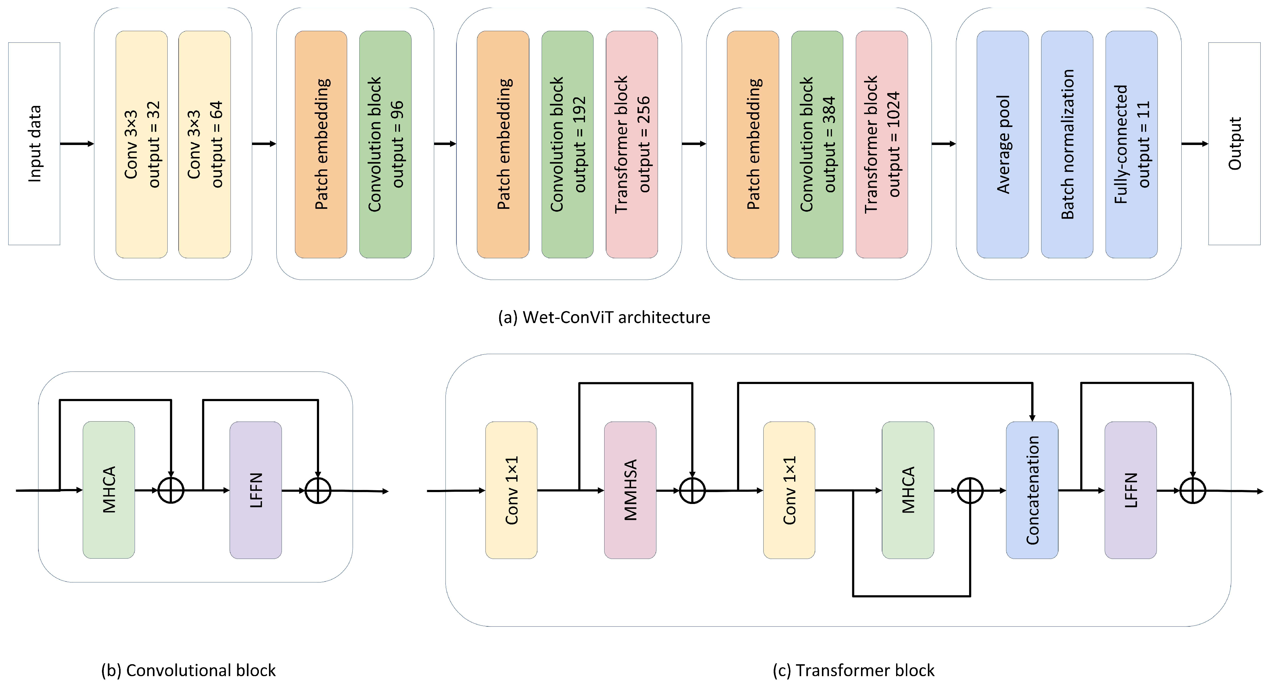
3.1. Proposed Framework

This study introduces a hybrid CNN–transformer model, namely Wet-ConViT, for wetland classification from satellite data. The architecture of Wet-ConViT includes patch embedding, transformer, and convolutional blocks (Figure 2). The model processes 14 layer inputs, comprising 10 from Sentinel-2 and 4 from Sentinel-1, using a patch size of 16 (determined through an experimental analysis detailed in Section 4.8). These inputs are initially passed through two convolutional layers with output sizes of 32 and 64, respectively. Following the initial processing, patch embedding is applied to capture multi-scale contextual information. The embedded data are then directed through multiple convolutional and local transformer blocks, enabling the extraction of both short- and long-range features. Accordingly, the data flow proceeds through a convolutional block with an output size of 96. The model then progresses through two consecutive blocks, each comprising patch embedding, convolutional block, and transformer block. The first block outputs 256 features, while the second block outputs 1024 features from the transformer blocks.

Within these convolutional and local transformer blocks, specialized modules, namely the modified multi-head self-attention (MMHSA), multi-head convolutional attention (MHCA), and local feed-forward network (LFFN), are employed to derive the desired features. MMHSA focuses on extracting low-frequency features, MHCA attends to local relationships among data tokens, and LFFN preserves locality in the feed-forward framework. This strategic integration ensures that Wet-ConViT can effectively capture both short-range spatial details and long-range dependencies inherent in wetland classification tasks.

After the feature extraction stages, the derived information is passed through batch normalization to stabilize and accelerate training, followed by average pooling to aggregate spatial information. Finally, a fully connected layer with an output size equal to the number of wetland classes (11 in this case) performs the classification for each pixel. Detailed information regarding the modules and blocks is summarized in the following subsections.

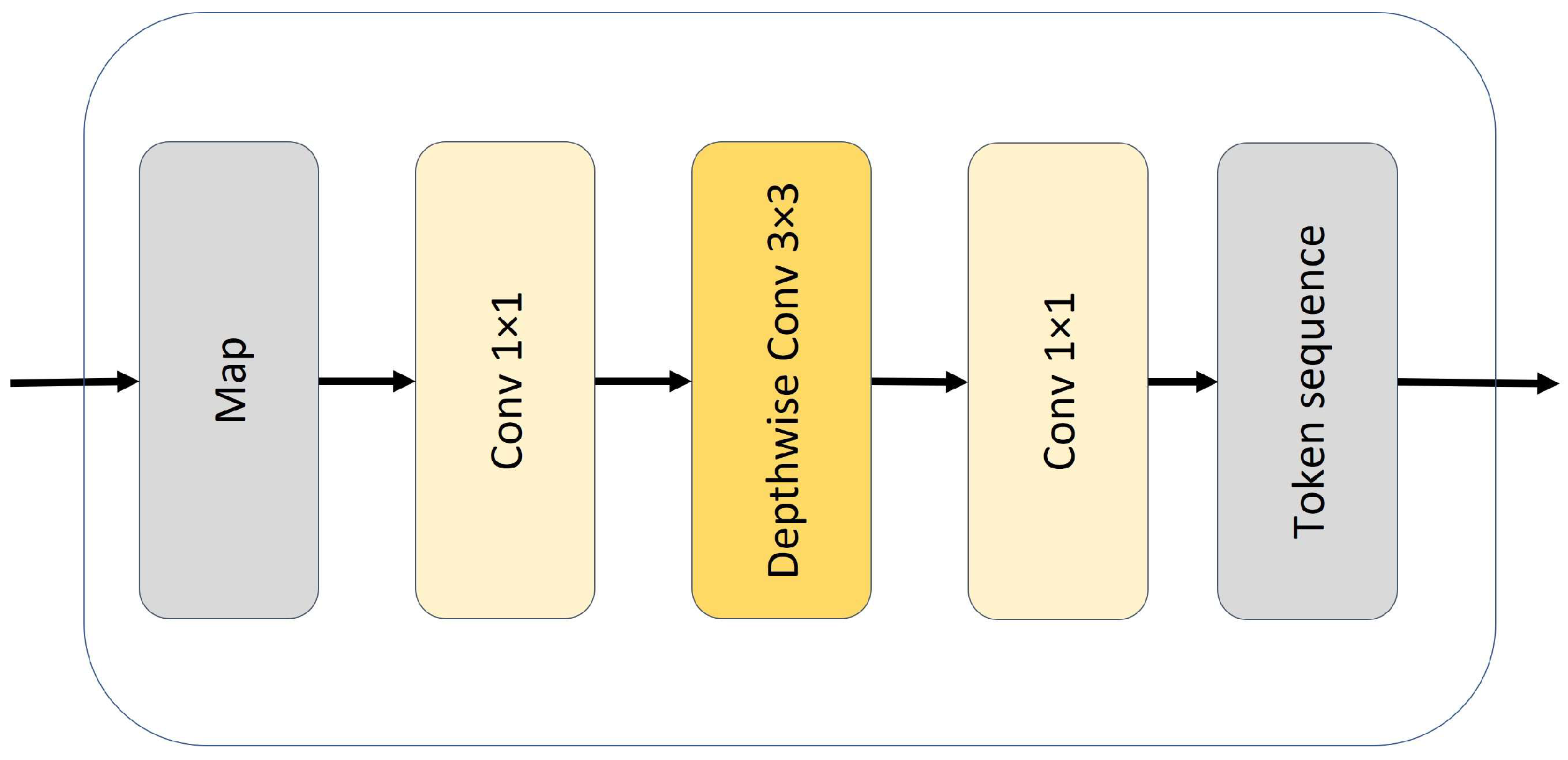
3.1.1. Modified Multi-Head Self-Attention (MMHSA)

The utilized modified multi-head self-attention (MMHSA) [53] module extracts low-frequency information with a reduced cost compared to a typical MHSA module. This module is composed of h parallel self-attentions to derive features from the input X, with subspaces of x₁, …, x_h to be fed to each head. The self-attention (SA) for input X can be calculated using Query, Key, and Value layer parameters (W^Q, W^K, W^V) as follows:

SA(X) = Attention(X·W^Q, P_s (X·W^K), P_s (X·W^V)),

(1)

The layer parameters in typical attention can be calculated using $softmax(Q K^T/\sqrt{d} V)$, where d is the hidden dimension of the transformer. In the modified version in Equation (1), there is an addition P_s parameter, which involves average-pooling downsampling operation with stride s. This parameter reduces the spatial dimension before the attention module and reduces the computational cost as well.

By concatenating the SAs of the parallel subspaces, the MMHSA can be calculated as follows:

$$\mathrm{MMHSA}(\mathrm{x})=\mathrm{concatenate}({\sum }_{\mathrm{i}=1}^{\mathrm{h}}{\mathrm{S}\mathrm{A}}_{\mathrm{i}}({\mathrm{x}}_{\mathrm{i}})){\mathrm{W}}^{\mathrm{O}}$$

(2)

where W^O is the output layer parameter. To further reduce the computational cost, a shrinking ratio parameter reduces the data dimension within a pointwise convolution. These modifications can improve the efficiency of the self-attention module, which is a critical factor in the computational complexity of the model.

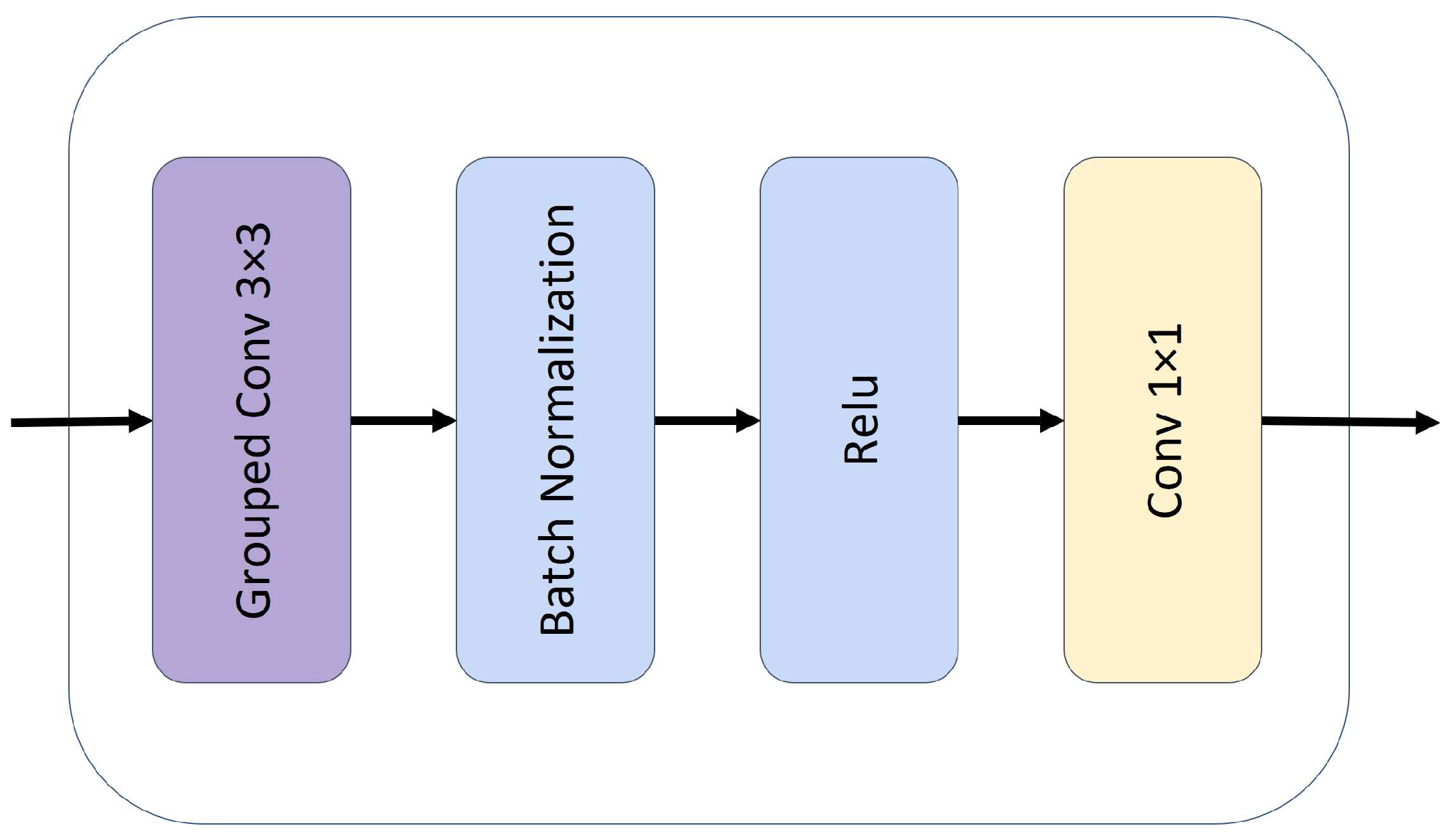
3.1.2. Multi-Head Convolutional Attention (MHCA)

Multi-head convolutional attention (MHCA) [53] is an attention mechanism levering the capabilities of convolutional operations. This module is designed to direct its attention to distinct representation subspaces across different regions, enabling the effective learning of local relationships. Within each of these subspaces, the calculation of single-head convolutional attention (CA) involves the utilization of a trainable parameter (W) and adjunct tokens (T_i,j) in the input data (X), as follows:

CA(X) = W·T_i,j, T_i,j∈X

(3)

The MHCA concatenates the single-head CAs from different subspaces (h) using a trainable weight (W^O):

$$\mathrm{MHCA}(\mathrm{x})=\mathrm{concatenate}({\sum }_{\mathrm{i}=1}^{\mathrm{h}}{\mathrm{C}\mathrm{A}}_{\mathrm{i}}({\mathrm{x}}_{\mathrm{i}})){\mathrm{W}}^{\mathrm{O}}$$

(4)

The MHCA module captures the local relationships among tokens. This module is constructed using a group convolution operation with a kernel size of 3, which is succeeded by batch normalization, the ReLU activation function, and a pointwise convolution with a size of 1 (Figure 3). In other words, the group convolution operation implements the multi-head step by taking adjacent tokens as input. Group convolutions involve partitioning the data into several groups and then applying separate kernels to each group. This approach effectively reduces the computational cost associated with conventional convolution operations [54].

3.1.3. Local Feed-Forward Network (LFFN)

Local feed-forward network (LFFN) [53] considers the locality in a feed-forward framework, which is essential for accurately capturing spatial dependencies in remote sensing data. The LFFN addresses the challenge of preserving local information by converting the sequence of tokens into a feature map and preserving location information by placing tokens at pixel locations. The architecture of the LFFN, shown in Figure 4, involves passing the mapped sequences through 1 × 1 pointwise convolutions and a 3 × 3 depthwise convolution. This structure allows the LFFN to effectively capture local features and neighboring information.

The combination of pointwise convolutions and depthwise convolutions enables the LFFN to extract detailed local features. The pointwise convolutions help in reducing dimensionality while preserving essential information, and the depthwise convolutions focus on capturing spatial relationships within a small neighborhood.

By mapping sequences to a feature map and applying convolutions, the LFFN preserves the spatial relationships between pixels. This preservation is critical for maintaining the integrity of local features, which are often lost in traditional feed-forward networks. This preservation of local information ensures that the subsequent attention layers receive a rich representation of spatial features. This feed-forward network helps the model to consider the locality and neighboring information in a feed-forward architecture. The output is reverted back to its sequence format to be used in the next attention layers.

3.1.4. Convolutional and Local Transformer Blocks

The utilized convolutional block incorporates both an MHCA and an LFFN within a residual block framework (see Figure 2b). This hybrid design aims to efficiently capture short-range and local information. The convolutional block’s formulation is described by the following equations:

z₁^l = MHCA(z^l−1) + z^l−1

(5)

z^l = LFFN(z₁^l) + z₁^l

(6)

where z^l−1 and z^l donate the input and output of the l th convolution block, while z₁^l represents the output of the l th MHCA. The convolutional block leverages the transformer-like token mixing capability of the MHCA module and the locality aspects of the LFFN to extract low-frequency information from the satellite data.

The local transformer block combines MMHSA, MHCA, LFFN, and pointwise convolutions by using the capabilities of residual module structure (Figure 2c). This block is able to capture long-range dependencies using the MMHSA module efficiently. The formulation of the local transformer block is presented as follows:

z₁^l = conv(z^l−1)

(7)

z₂^l = MMHSA(z₁^l) + z₁^l

(8)

z₃^l = conv(z₂^l)

(9)

z₄^l = MHCA(z₃^l) + z₃^l

(10)

z₅^l = concatenate(z₂^l, z₄^l)

(11)

z^l = LFFN(z₅^l) + z₅^l

(12)

where z^l−1 and z^l represent the input and output of the l^th transformer block, while z₁^l to z₅^l denote the outputs of the respective transformer block layers. The conv() function indicates a pointwise convolutional layer.

The MHCA module is responsible for learning dependencies among tokens within short ranges, and the LFFN module improves the extraction of local information within the transformer block. The concatenation of MMHSA and MHCA within the transformer block combines both low and high-frequency information.

3.2. Evaluation Models and Metrics

We compared the proposed Wet-ConViT model’s performance with multiple state-of-the-art deep learning models, including convolutional, transformer, and hybrid architectures, in order to evaluate its potential for classifying wetland areas. These models include ResNet50 [55] and EfficientNet-V2 [56] from the CNN category, ViT [42] and Swin-v2 [44] from the transformers, and CvT [57], CoAtNet [58], and WetMapFormer (WMF) [19] from the hybrid category. To ensure a more effective comparison with the proposed model, we deliberately opted for the smallest version of each model among their various existing variants. This approach allows for a closer match in terms of model parameters and processing time when compared to the proposed model. As such, we considered the small version of EfficientNet-V2, the base version of ViT, the tiny version of Swin-V2, CvT-13, and CoAtNet-0.

Next, the efficiency of the deep learning models is examined in terms of both accuracy metrics and computational complexity. Model complexity is a crucial consideration, particularly in large-scale applications. Various factors serve as indicators of model complexity, with key metrics being the number of parameters (Params) and training time. Params represent the number of trainable parameters involved in the training process.

The per-class accuracy of the models is assessed using the F1-Score (F1), along with three overall metrics: overall accuracy (OA), average accuracy (AA), and the kappa coefficient (k), to evaluate the performance of the models in wetland classification. The per-class F1 can be calculated based on precision (P), recall (R), and confusion matrix elements, as follows:

P = TP/TP + FP

(13)

R = TP/TP + FN

(14)

F1-score = 2 × (P × R)/(P + R)

(15)

True positive (TP) is the number of correctly classified samples for a specific land cover class, whereas false positive (FP) and false negative (FN) signify the number of samples incorrectly predicted as a particular category (positive) and as different categories (negative), respectively. These metrics can be defined using the following equations:

OA = N_Correct/N_Total

(16)

$$\mathrm{AA}=({\sum }_{\mathrm{i}=1}^{\mathrm{C}}{\mathrm{R}}_{\mathrm{i}})/\mathrm{C}$$

(17)

$$\mathrm{k}=(\mathrm{OA}-{\mathrm{P}}_{\mathrm{e}})/(1-{\mathrm{P}}_{\mathrm{e}}); \mathrm{where} {\mathrm{P}}_{\mathrm{e}}=({\sum }_{\mathrm{i}=1}^{\mathrm{C}}({{\mathrm{N}}^{\mathrm{i}}}_{\mathrm{True}}+{{\mathrm{N}}^{\mathrm{i}}}_{\mathrm{Predict}}))/{\mathrm{N}}_{{\mathrm{Total}}^2}$$

(18)

where C represents the total number of classes, and R_i donates the recall (R) of the i^th class. Nⁱ_True and Nⁱ_Predict stand for the number of true samples (TP + FN) and correctly predicted samples (TP + TN) within class i, respectively. N_Correct and N_Total represent the number of correct predictions and total number of samples.

4. Experiments and Results

4.1. Implementation Details

The experiments were conducted on the PyTorch platform (version 2.3), utilizing a Tesla T4 GPU with 12 GB of VRAM. The specific environment included CUDA version 12.1 and CuDNN version 8.9.6. The deep learning models were trained over 50 epochs with a fixed learning rate of 1 × 10⁻⁴, which were selected based on preliminary experiments and validation performance. The error for each epoch was computed using the cross-entropy loss function and optimized using the Adam optimizer [59]. The input patch size of 16 × 16 was determined through experimental analysis (Section 4.8).

A stratified K-fold sampling technique was employed to validate the performance of the classification methods. In this approach, K = 3 was considered to provide a balance between training and testing datasets. Each of the three folds was designed to contain an approximately equal number of samples, ensuring a nearly uniform distribution of samples across each class within every fold.

To achieve this, we spatially distributed the samples such that the first fold primarily included samples from the northern part of the study area, the second fold included samples from the middle, and the third fold included samples from the southern part. This spatial distribution reduces the spatial dependency of samples between folds, thus reducing the spatial dependency of the train and test samples, leading to a more rigorous validation of model performance.

For thorough evaluation, we repeated the K-fold procedure five times for each model, resulting in a total of 15 training iterations. In each training iteration, one fold (approximately 33% of the data) was left out for testing, while the remaining two folds (approximately 67% of the data) were used for training. This process ensured that each sample was used for both training and testing, enhancing the robustness of the validation. Furthermore, within the training samples, 10,000 samples (approximately 5%) were randomly selected for validation, employing a stratified random sampling technique. This ensured that the validation set was also representative of the overall class distribution, providing a reliable measure of model performance during training.

This stratified K-fold validation approach ensures a well-balanced distribution of training and testing samples, enhancing the reliability of our assessment. By spatially and statistically distributing the samples across the folds, land covers, and iterations, we can more rigorously assess the generalizability and robustness of our classification methods.

4.2. Classification Maps

The classified wetland map produced by the Wet-ConViT model over the study area is depicted in Figure 5. Different land covers are classified into wetland and non-wetland categories on this map. In order to evaluate the performance of the proposed model, a zoom-in-area covering the North and East end of St. John’s is considered for visual interpretation and comparison with classification maps of other state-of-the-art DL models (Figure 6).

Overall, all models successfully identified the primary features and land cover types; however, each approach encountered specific challenges. The classification of marshland covers emerged as the most challenging task across the classified maps. In particular, CNN-based (i.e., Resnet50 and EfficientNet) classification maps underestimated this wetland category, whereas transformer-based models (i.e., ViT and Swin) represented an overestimation of this particular category. This overestimation issue was especially noticeable in the Swin model’s results, where some regions saturated with lake water were incorrectly categorized as marshlands. Despite challenges in classifying water bodies within the transformer models, this category exhibited the highest degree of consistency across all predicted maps. An additional challenge observed with the transformer model was the classification of bog and fen wetland covers. In certain instances, these wetland types were erroneously identified as pasture, notably in the northern part of the study area.

The category of urban land cover was effectively identified by most models, although some, like the CvT model, overestimated this category. The CvT model, while preserving many details in urban areas, occasionally misclassified grasslands and pastures as urban land. On the other hand, the hybrid CoAtNet model encountered overestimation challenges when classifying swamps, leading to the misclassification of numerous grassland and urban areas as swamps. The WMF model output map preserved details but showed an underestimation of bog and swamp land cover in the northern part of the study area. It also slightly overestimated forest land cover. As illustrated, the proposed model yielded a more homogenous land cover map with less noise while still preserving the key features of land cover classes.

4.3. UMAP Feature Distribution

For a comprehensive visual assessment of the feature extraction capability of the DL models, a uniform manifold approximation and projection (UMAP) technique was considered [60]. UMAP is a dimensionality reduction technique that projects high-dimensional data into a lower-dimensional space, typically 2D or 3D while preserving the global structure and local relationships of the data. This technique is particularly useful for visualizing complex patterns and distributions in the data, allowing for an intuitive understanding of how well different models separate various land cover classes. The resulting 2-dimensional feature distributions, obtained through UMAP, are illustrated in Figure 7.

The UMAP visualizations revealed the remarkable potential of all models in distinguishing water and urban from other land covers, verifying the observations of the visual interpretation of classification maps. However, for the remaining land cover categories, particularly bog, fen, and swamp wetland land covers, the 2D feature distributions exhibited substantial overlap, making their differentiation challenging. The hybrid models demonstrated superior performance in separating these wetland classes when compared to CNNs and transformers. The overlap between sub-wetland categories is still high for CvT and WMF, with CoAtNet and the proposed model showing better performance distinguishing wetland subcategories. The UMAP representation of the proposed model demonstrated the highest level of separability for distinguishing these wetland subclasses. For example, marsh and water land covers exhibited closely overlapping distributions for most DL models, as shown by the classification maps, yet our proposed model demonstrates the highest degree of separability for these classes.

In addition to wetland classes, the separation of pasture and grassland categories presented its own set of challenges. These classes often share similar spectral characteristics, leading to overlapping feature distributions. Nevertheless, the hybrid models, particularly the proposed Wet-ConViT, excelled in effectively separating these classes. The enhanced separability observed in the UMAP visualizations for the proposed model can be attributed to its ability to capture both local and global features, thanks to the combined use of convolutional and transformer blocks.

The detailed interpretation of the UMAP feature distribution results, alongside the classification maps and statistical results (in Section 4.5), provides a comprehensive understanding of how the proposed model achieves superior performance. The separability of different land cover classes in UMAP visualizations demonstrates the effectiveness of the proposed Wet-ConViT model in accurately classifying complex wetland and non-wetland categories.

4.4. Statistical Results

The proposed Wet-ConViT model’s per-class accuracy and overall accuracy metrics are thoroughly examined and compared to those of other current state-of-the-art models, as shown in

Table 2. Per-class and overall accuracy metrics of the deployed classification models for wetland classification (the highest accuracies per class and overall metric are shown in bold).

	Models
	Convolution		Transformer		Hybrid
Class	ResNet50	EfficientNet	ViT	Swin	CvT	CoAtNet	WMP	Proposed
Bog	90.14%	89.07%	81.94%	88.87%	90.71%	92.15%	88.15%	94.79%
Fen	83.29%	82.61%	78.14%	81.19%	84.63%	86.85%	82.45%	90.57%
Swamp	80.66%	79.81%	73.93%	75.56%	79.01%	84.47%	81.37%	89.04%
Marsh	75.80%	79.42%	79.59%	76.91%	84.94%	89.52%	82.03%	89.91%
Water	98.66%	98.62%	98.97%	98.63%	99.07%	99.21%	99.43%	99.02%
Forests	90.52%	90.34%	87.32%	89.20%	90.94%	94.29%	91.09%	95.96%
Shrublands	88.35%	87.61%	84.46%	85.56%	91.29%	96.66%	88.18%	94.88%
Grassland	82.86%	82.77%	78.15%	79.45%	83.29%	89.75%	85.89%	93.41%
Pastures	93.89%	94.93%	92.23%	91.71%	93.74%	95.40%	96.33%	98.08%
Barren	92.33%	89.85%	92.35%	86.20%	82.03%	98.66%	94.63%	94.23%
Urban	98.77%	98.32%	98.90%	97.90%	98.44%	99.21%	99.13%	99.46%
OA	90.39%	90.18%	87.05%	88.75%	90.82%	93.34%	90.91%	95.36%
AA	88.66%	88.49%	86.00%	86.47%	88.92%	93.29%	88.84%	94.49%
k	89.08%	88.82%	85.26%	87.22%	89.56%	92.44%	89.64%	94.72%

. The results of this comparative analysis indicate the remarkable performance of the Wet-ConViT model, outperforming other models in terms of overall accuracy metrics and the majority of the land cover categories. However, the hybrid CoAtNet model demonstrated higher accuracies for some non-wetland classes, such as shrubland and barren land covers. The results revealed that the combination of convolutional and transformer components within the hybrid models yielded the highest accuracy compared to the single network architecture (either convolutional or transformer). However, convolutional layers were found to be more successful compared to transformers for classifying land covers, achieving an approximate overall accuracy of 90% with both ResNet50 and EfficientNet. This could be attributed to the better capability of CNNs in extracting local features, a key factor in land cover classification tasks that may be overlooked by transformers. This improvement was noticeable across all overall and most per-class accuracy metrics.

4.5. Result Analysis and Discussion

The statistical results (presented in Table 2) indicate the superior performance of the proposed Wet-ConViT model across various land cover classes and overall accuracy metrics. The proposed model achieved the highest accuracies for bog (94.79%), fen (90.57%), swamp (89.04%), and marsh (89.91%), which are challenging wetland classes. In comparison, other models showed lower accuracies for these classes, highlighting the effectiveness of the proposed hybrid approach in capturing both local and global features essential for accurate wetland classification.

As discussed earlier (on both classification maps and UMAPs in Figure 6 and Figure 7), the classes of water and urban are the most discernible categories, achieving accuracies surpassing 97% across all models. Particularly, the proposed model demonstrated exceptional potential, achieving accuracies exceeding 99% for both of these categories. Conversely, the marsh and swamp land covers presented to be the most challenging classes to be distinguished in both classification maps and UMAPs and consistently yield the lowest accuracies.

The overlap in spectral features between marsh, swamp, and water reflected in the spectral feature overlap seen in UMAP results (Figure 7), as well as their proximity to each other (shown in classification maps in Figure 6), led to confusion among these categories. Accordingly, both state-of-the-art and proposed models struggled with these classes and resulted in the lowest accuracies among all the land covers. Despite these challenges, the proposed model attained accuracy rates exceeding 89% for these wetland categories.

Among the non-wetland land covers, grassland showed the lowest accuracy, which only the proposed model could achieve above 90% accuracy. As evident in classification maps (Figure 6), grasslands are the dominant land covers in the northern part of the study area, where they coexist along the urban area of the city of St. John’s. The separability of these land covers is limited by the spatial resolution of the input data. The presence of mixed pixels, where more than one land cover type is present within a single pixel, further complicates accurate classification. Moreover, grassland-extracted features overlap with the pasture category (as evident in UMAP Figure 7). This inherent heterogeneity and spatial distribution of land covers add complexity to the classification task.

The spectral similarity between certain classes, as well as the spatial resolution of the input data, influenced the classification accuracy. The overlap in spectral features often led to confusion between these classes. Furthermore, the spatial distribution and heterogeneity of land covers, especially in transitional zones, posed additional challenges. The use of both convolutional and transformer blocks improved the classification performance of our hybrid model by capturing both local and global patterns. Additionally, the use of the LFFN module helps to better preserve spatial features within different blocks of the model. Overall, the accuracy metrics support the visual interpretation of our findings, highlighting the superior performance of the Wet-ConViT model for classifying wetlands.

4.6. Impact of Multi-Source Satellite Data

To determine the influence of multispectral Sentinel-2 (S2) and Synthetic Aperture Radar Sentinel-1 (S1) data on the classification results obtained by the Wet-ConViT model, we conducted an ablation study, extending this analysis to other hybrid models as well. As represented in

Table 3. Ablation results on different satellite data sources.

	S1				S2				S1S2
Class	CvT	CoAtNet	WMF	Proposed	CvT	CoAtNet	WMF	Proposed	CvT	CoAtNet	WMF	Proposed
Bog	70.41%	81.89%	58.56%	79.79%	81.60%	83.22%	79.86%	93.78%	90.71%	92.15%	88.15%	94.79%
Fen	61.47%	75.63%	54.44%	72.88%	79.99%	79.26%	78.46%	89.19%	84.63%	86.85%	82.45%	90.57%
Swamp	50.37%	65.07%	28.62%	68.36%	67.46%	71.90%	70.34%	86.63%	79.01%	84.47%	81.37%	89.04%
Marsh	64.57%	73.84%	48.72%	79.11%	48.44%	59.78%	51.98%	87.73%	84.94%	89.52%	82.03%	89.91%
Water	96.80%	96.49%	95.73%	97.75%	97.25%	98.52%	98.14%	97.83%	99.07%	99.21%	99.43%	99.02%
Forests	72.28%	82.66%	72.58%	85.36%	80.93%	85.03%	85.29%	94.06%	90.94%	94.29%	91.09%	95.96%
Shrublands	56.78%	67.09%	46.79%	67.56%	85.72%	83.40%	87.33%	90.98%	91.29%	96.66%	88.18%	94.88%
Grassland	52.39%	65.76%	16.41%	70.36%	77.26%	79.86%	79.35%	90.14%	83.29%	89.75%	85.89%	93.41%
Pastures	85.89%	91.33%	84.11%	91.46%	85.29%	90.79%	90.89%	96.51%	93.74%	95.40%	96.33%	98.08%
Barren	60.53%	73.73%	30.16%	72.39%	39.24%	45.81%	72.22%	92.31%	82.03%	98.66%	94.63%	94.23%
Urban	84.97%	93.37%	86.08%	90.47%	94.85%	94.78%	94.49%	98.74%	98.44%	99.21%	99.13%	99.46%
OA	72.43%	82.36%	67.52%	82.56%	82.23%	84.42%	83.89%	93.73%	90.82%	93.34%	90.91%	95.36%
AA	69.51%	78.79%	56.62%	80.78%	77.37%	81.93%	79.43%	92.75%	88.92%	93.29%	88.84%	94.49%
k	68.77%	79.95%	62.77%	80.18%	79.75%	82.23%	81.59%	92.87%	89.56%	92.44%	89.64%	94.72%

, the result of this analysis revealed that using only the S2 dataset yields significantly higher accuracies for all land cover categories when compared to the S1 dataset. For the proposed model, the single use of S2 data obtained an overall accuracy of approximately 93%, which is 11% higher than that obtained with a single source S1 dataset. Similar trends were observed for other hybrid models, although the proposed Wet-ConViT consistently outperformed them.

When using S1 data, the proposed Wet-ConViT model showed superior performance with an OA of 82.56%, outperforming other models such as CoAtNet (82.36%) and WMF (67.52%). This highlights the effectiveness of the proposed model in leveraging SAR data for wetland classification tasks. In comparison, CvT and CoAtNet models demonstrated moderate performance, with CoAtNet achieving relatively higher accuracy among these models.

For S2 data, the proposed model achieved 93.73% OA, which was significantly higher than the OAs of CoAtNet (84.42%) and CvT (82.23%). WMF showed competitive results with other hybrid models achieving an OA of 83.89%, still falling behind the proposed model. These results indicate the robustness of the proposed model in effectively utilizing multispectral data for improved classification accuracy.

The combination of S1 and S2 data (S1S2) yielded the highest overall performance for all models. These improvements can be attributed primarily to the distinct, complementary information provided by SAR data. While SAR data alone showed inferior capability compared to optical data, it serves as a valuable source of information in the classification task by playing a key role in discriminating categories with similar optical features. For example, despite the close optical feature distribution of shrubland and grassland categories, the combined dataset led to notable enhancements for the separation of these classes, attaining 3–4% improvements for the proposed model. This could be attributed to the greater capability of SAR data compared to optical data in capturing different soil and canopy moisture levels within shrublands and grasslands, thus enabling a better separation of these two classes [61,62]. The complementary utilization of multi-source satellite data not only leverages the strengths of each but also compensates for their individual limitations, thereby highlighting the importance of their combined application in remote sensing.

The results indicated that the proposed Wet-ConViT model achieved the highest performance among all tested models, even when using single-source data. For example, using only S2 data, the proposed model achieved 93.73% OA, whereas the second-best model, CoAtNet, achieved 84.42% OA. This demonstrates the superior capability of the proposed Wet-ConViT model in effectively utilizing multi-source satellite data for enhanced classification accuracy.

4.7. Efficiency Analysis

The proposed Wet-ConViT model exhibits a remarkable performance in accurately classifying various wetland land covers. One critical factor to be considered, particularly in large-scale applications, is the efficiency of deep learning (DL) models in terms of memory usage and processing time. This challenge was taken into account during the design of the Wet-ConViT architecture, with the aim of achieving the highest accuracy while minimizing the number of parameters and optimizing processing time.

To assess the efficiency of the proposed model, a comparative analysis was conducted between the proposed model and other state-of-the-art models in terms of four factors: the number of parameters (in millions), memory size (in MB), average training time per epoch (in seconds), and inference time (in seconds). The results are summarized in

Table 4. Efficiency analysis of the DL models.

	ResNet50	EfficientNet	ViT	Swin	CvT	CoAtNet	WMF	Proposed
Params (millions)	23.57	20.19	87.72	27.61	19.66	17.37	0.7	9.44
Memory size (MB)	90.2	77.9	335.1	105.8	75.3	66.4	8.3	36.3
Training time (s)	63	122	122	276	116	75	37	77
Inference time (s)	5.99	13.64	13.08	32.99	19.73	15.55	3.07	9.16
OA (%)	90.39	90.18	87.05	88.75	90.82	93.34	90.91	95.36

.

Among the deployed DL models, the proposed model comprises a relatively low number of parameters and memory size, the second after WMF. The proposed model’s number of parameters and memory size are approximately half of the second-best model, CoAtNet, along with a 2% improvement in terms of overall accuracy. The memory size is a crucial factor for evaluating the efficiency of models, especially for deployment in resource-constrained environments. The relatively low size of the proposed model (36.3 MB) makes it more suitable for real-time applications and scenarios where computational resources are limited.

Training time and inference time are crucial factors for evaluating the efficiency of models in practical applications. The proposed Wet-ConViT model has an average training time of 77 s per epoch, which is competitive compared to other models such as CoAtNet (75 s) and significantly faster than transformer models. Although ResNet50 demonstrates a relatively short training time per epoch (63 s), it demands considerably more memory and falls behind the Wet-ConViT model in terms of overall accuracy metrics (~5%). Regarding inference time, the proposed model has an inference time of 9.16 s, which, although not the fastest, strikes a balance between speed and accuracy. WMF exhibits the fastest inference time (3.07 s) but is less accurate compared to the proposed model (~5%). The proposed model’s inference time is acceptable for real-time applications while offering superior classification performance.

4.8. Patch Size Effect

The proposed model requires a minimum patch size of 8 x 8; nevertheless, increasing the patch size has the potential to improve classification accuracy with a higher computational cost. To determine the optimal balance between accuracy and computational complexity, the model’s performance was evaluated with different patch sizes ranging from 8 to 20 in Figure 8. This analysis revealed that patch sizes exceeding 16 × 16 yield a negligible improvement in OA (less than 0.03%); however, they also exhibit a drastic rise in processing time (about 24 s increase per training epoch). Accordingly, a patch size of 16 was identified as the optimum patch size, maintaining an effective balance between accuracy and computational cost.

5. Conclusions

In this research, a novel deep learning architecture for mapping wetlands was introduced by harnessing a combination of multi-source satellite data, including multispectral Sentinel-2 and Sentinel-1 SAR datasets. The proposed model, called Wet-ConViT, has been developed with the primary objective of achieving precise land cover classification while minimizing computational complexity.

The proposed model leverages the capabilities of both convolutions for capturing local information and transformers for capturing the long-range dependencies of extracted features. Accordingly, a multi-head convolutional attention module (MHCA), a modified version of multi-head self-attention, and a local feed-forward network (LFFN) were used in the Wet-ConViT model within convolutional and transformer blocks. These integrated modules and blocks reduce the computational complexity associated with vanilla transformers and enhance the models’ ability to incorporate local contextual information, thereby contributing to the overall efficiency and improved classification accuracy of the model.

The performance of our proposed Wet-ConViT model was compared to several state-of-the-art CNNs, transformers, and hybrid models. The results demonstrated the superiority of the proposed model compared to other state-of-the-art models in terms of accuracy metrics and parameter efficiency. Although WMF exhibited the best efficiency in terms of inference time and memory usage, it fell short by approximately 5% in classification accuracy compared to the proposed model. Moreover, the second-best model in terms of accuracy, CoAtNet, required significantly larger memory and longer inference time, making the proposed model more balanced for practical applications.

The Wet-ConViT model represents a notable achievement in maintaining a delicate balance between efficiency and accuracy in the context of complex land cover classification. Its superior performance, coupled with its efficiency in terms of parameters, memory, and processing time, underscores its value as an exemplary model for practical applications in wetland classification tasks.

References

1. Jamali, A.; Mahdianpari, M.; Mohammadimanesh, F.; Homayouni, S. A Deep Learning Framework Based on Generative Adversarial Networks and Vision Transformer for Complex Wetland Classification Using Limited Training Samples. Int. J. Appl. Earth Obs. Geoinf. 2022, 115, 103095. [Google Scholar] [CrossRef]
2. Jamali, A.; Mahdianpari, M. Swin Transformer and Deep Convolutional Neural Networks for Coastal Wetland Classification Using Sentinel-1, Sentinel-2, and LiDAR Data. Remote Sens. 2022, 14, 359. [Google Scholar] [CrossRef]
3. Jaramillo, F.; Brown, I.; Castellazzi, P.; Espinosa, L.; Guittard, A.; Hong, S.-H.; Rivera-Monroy, V.H.; Wdowinski, S. Assessment of Hydrologic Connectivity in an Ungauged Wetland with InSAR Observations. Environ. Res. Lett. 2018, 13, 024003. [Google Scholar] [CrossRef]
4. Adeli, S.; Salehi, B.; Mahdianpari, M.; Quackenbush, L.J.; Brisco, B.; Tamiminia, H.; Shaw, S. Wetland Monitoring Using SAR Data: A Meta-Analysis and Comprehensive Review. Remote Sens. 2020, 12, 2190. [Google Scholar] [CrossRef]
5. Hosseiny, B.; Mahdianpari, M.; Brisco, B.; Mohammadimanesh, F.; Salehi, B. WetNet: A Spatial–Temporal Ensemble Deep Learning Model for Wetland Classification Using Sentinel-1 and Sentinel-2. IEEE Trans. Geosci. Remote Sens. 2022, 60, 4406014. [Google Scholar] [CrossRef]
6. Mitsch, W.J.; Bernal, B.; Hernandez, M.E. Ecosystem Services of Wetlands. Int. J. Biodivers. Sci. Ecosyst. Serv. Manag. 2015, 11, 1–4. [Google Scholar] [CrossRef]
7. Jamali, A.; Mahdianpari, M. Swin Transformer for Complex Coastal Wetland Classification Using the Integration of Sentinel-1 and Sentinel-2 Imagery. Water 2022, 14, 178. [Google Scholar] [CrossRef]
8. Costanza, R.; De Groot, R.; Sutton, P.; Van Der Ploeg, S.; Anderson, S.J.; Kubiszewski, I.; Farber, S.; Turner, R.K. Changes in the Global Value of Ecosystem Services. Glob. Environ. Change 2014, 26, 152–158. [Google Scholar] [CrossRef]
9. Serran, J.N.; Creed, I.F.; Ameli, A.A.; Aldred, D.A. Estimating Rates of Wetland Loss Using Power-Law Functions. Wetlands 2018, 38, 109–120. [Google Scholar] [CrossRef]
10. Mahdianpari, M.; Granger, J.E.; Mohammadimanesh, F.; Salehi, B.; Brisco, B.; Homayouni, S.; Gill, E.; Huberty, B.; Lang, M. Meta-Analysis of Wetland Classification Using Remote Sensing: A Systematic Review of a 40-Year Trend in North America. Remote Sens. 2020, 12, 1882. [Google Scholar] [CrossRef]
11. Holland, R.A.; Darwall, W.R.T.; Smith, K.G. Conservation Priorities for Freshwater Biodiversity: The Key Biodiversity Area Approach Refined and Tested for Continental Africa. Biol. Conserv. 2012, 148, 167–179. [Google Scholar] [CrossRef]
12. Onojeghuo, A.O.; Onojeghuo, A.R. Wetlands Mapping with Deep ResU-Net CNN and Open-Access Multisensor and Multitemporal Satellite Data in Alberta’s Parkland and Grassland Region. Remote Sens Earth Syst Sci 2023, 6, 22–37. [Google Scholar] [CrossRef]
13. Cho, M.S.; Qi, J. Characterization of the Impacts of Hydro-Dams on Wetland Inundations in Southeast Asia. Sci. Total Environ. 2023, 864, 160941. [Google Scholar] [CrossRef]
14. Fu, B.; Zuo, P.; Liu, M.; Lan, G.; He, H.; Lao, Z.; Zhang, Y.; Fan, D.; Gao, E. Classifying Vegetation Communities Karst Wetland Synergistic Use of Image Fusion and Object-Based Machine Learning Algorithm with Jilin-1 and UAV Multispectral Images. Ecol. Indic. 2022, 140, 108989. [Google Scholar] [CrossRef]
15. Singh, M.; Allaka, S.; Gupta, P.K.; Patel, J.G.; Sinha, R. Deriving Wetland-Cover Types (WCTs) from Integration of Multispectral Indices Based on Earth Observation Data. Environ. Monit. Assess. 2022, 194, 878. [Google Scholar] [CrossRef]
16. Mahdianpari, M.; Motagh, M.; Akbari, V.; Mohammadimanesh, F.; Salehi, B. A Gaussian Random Field Model for De-Speckling of Multi-Polarized Synthetic Aperture Radar Data. Adv. Space Res. 2019, 64, 64–78. [Google Scholar] [CrossRef]
17. Chang, S.; Deng, Y.; Zhang, Y.; Zhao, Q.; Wang, R.; Zhang, K. An Advanced Scheme for Range Ambiguity Suppression of Spaceborne SAR Based on Blind Source Separation. IEEE Trans. Geosci. Remote Sens. 2022, 60, 5230112. [Google Scholar] [CrossRef]
18. Slagter, B.; Tsendbazar, N.-E.; Vollrath, A.; Reiche, J. Mapping Wetland Characteristics Using Temporally Dense Sentinel-1 and Sentinel-2 Data: A Case Study in the St. Lucia Wetlands, South Africa. Int. J. Appl. Earth Obs. Geoinf. 2020, 86, 102009. [Google Scholar] [CrossRef]
19. Jamali, A.; Roy, S.K.; Ghamisi, P. WetMapFormer: A Unified Deep CNN and Vision Transformer for Complex Wetland Mapping. Int. J. Appl. Earth Obs. Geoinf. 2023, 120, 103333. [Google Scholar] [CrossRef]
20. Franklin, S.E.; Skeries, E.M.; Stefanuk, M.A.; Ahmed, O.S. Wetland Classification Using Radarsat-2 SAR Quad-Polarization and Landsat-8 OLI Spectral Response Data: A Case Study in the Hudson Bay Lowlands Ecoregion. Int. J. Remote Sens. 2018, 39, 1615–1627. [Google Scholar] [CrossRef]
21. Wang, C.; Pavelsky, T.M.; Kyzivat, E.D.; Garcia-Tigreros, F.; Podest, E.; Yao, F.; Yang, X.; Zhang, S.; Song, C.; Langhorst, T.; et al. Quantification of Wetland Vegetation Communities Features with Airborne AVIRIS-NG, UAVSAR, and UAV LiDAR Data in Peace-Athabasca Delta. Remote Sens. Environ. 2023, 294, 113646. [Google Scholar] [CrossRef]
22. Xiang, H.; Xi, Y.; Mao, D.; Mahdianpari, M.; Zhang, J.; Wang, M.; Jia, M.; Yu, F.; Wang, Z. Mapping Potential Wetlands by a New Framework Method Using Random Forest Algorithm and Big Earth Data: A Case Study in China’s Yangtze River Basin. Glob. Ecol. Conserv. 2023, 42, e02397. [Google Scholar] [CrossRef]
23. Mahdianpari, M.; Mohammadimanesh, F. Applying GeoAI for Effective Large-Scale Wetland Monitoring. In Advances in Machine Learning and Image Analysis for GeoAI; Elsevier: Amsterdam, The Netherlands, 2024; pp. 281–313. ISBN 978-0-443-19077-3. [Google Scholar]
24. Mohammadimanesh, F.; Salehi, B.; Mahdianpari, M.; Gill, E.; Molinier, M. A New Fully Convolutional Neural Network for Semantic Segmentation of Polarimetric SAR Imagery in Complex Land Cover Ecosystem. ISPRS J. Photogramm. Remote Sens. 2019, 151, 223–236. [Google Scholar] [CrossRef]
25. Wang, X.; Jiang, W.; Deng, Y.; Yin, X.; Peng, K.; Rao, P.; Li, Z. Contribution of Land Cover Classification Results Based on Sentinel-1 and 2 to the Accreditation of Wetland Cities. Remote Sens. 2023, 15, 1275. [Google Scholar] [CrossRef]
26. Peng, K.; Jiang, W.; Hou, P.; Wu, Z.; Ling, Z.; Wang, X.; Niu, Z.; Mao, D. Continental-Scale Wetland Mapping: A Novel Algorithm for Detailed Wetland Types Classification Based on Time Series Sentinel-1/2 Images. Ecol. Indic. 2023, 148, 110113. [Google Scholar] [CrossRef]
27. Mahdavi, S.; Salehi, B.; Granger, J.; Amani, M.; Brisco, B.; Huang, W. Remote Sensing for Wetland Classification: A Comprehensive Review. GIScience Remote Sens. 2018, 55, 623–658. [Google Scholar] [CrossRef]
28. Amani, M.; Salehi, B.; Mahdavi, S.; Granger, J. Spectral analysis of wetlands in newfoundland using sentinel 2a and landsat 8 imagery. In Proceedings of the IGTF, Baltimore, MD, USA, 12–16 March 2017. [Google Scholar]
29. Jamali, A.; Mahdianpari, M.; Brisco, B.; Granger, J.; Mohammadimanesh, F.; Salehi, B. Deep Forest Classifier for Wetland Mapping Using the Combination of Sentinel-1 and Sentinel-2 Data. GIScience Remote Sens. 2021, 58, 1072–1089. [Google Scholar] [CrossRef]
30. Wang, M.; Mao, D.; Wang, Y.; Xiao, X.; Xiang, H.; Feng, K.; Luo, L.; Jia, M.; Song, K.; Wang, Z. Wetland Mapping in East Asia by Two-Stage Object-Based Random Forest and Hierarchical Decision Tree Algorithms on Sentinel-1/2 Images. Remote Sens. Environ. 2023, 297, 113793. [Google Scholar] [CrossRef]
31. Jafarzadeh, H.; Mahdianpari, M.; Gill, E.W.; Mohammadimanesh, F. Enhancing Wetland Mapping: Integrating Sentinel-1/2, GEDI Data, and Google Earth Engine. Sensors 2024, 24, 1651. [Google Scholar] [CrossRef]
32. Munizaga, J.; García, M.; Ureta, F.; Novoa, V.; Rojas, O.; Rojas, C. Mapping Coastal Wetlands Using Satellite Imagery and Machine Learning in a Highly Urbanized Landscape. Sustainability 2022, 14, 5700. [Google Scholar] [CrossRef]
33. Islam, M.K.; Simic Milas, A.; Abeysinghe, T.; Tian, Q. Integrating UAV-Derived Information and WorldView-3 Imagery for Mapping Wetland Plants in the Old Woman Creek Estuary, USA. Remote Sens. 2023, 15, 1090. [Google Scholar] [CrossRef]
34. Mahdianpari, M.; Salehi, B.; Mohammadimanesh, F.; Brisco, B.; Homayouni, S.; Gill, E.; DeLancey, E.R.; Bourgeau-Chavez, L. Big Data for a Big Country: The First Generation of Canadian Wetland Inventory Map at a Spatial Resolution of 10-m Using Sentinel-1 and Sentinel-2 Data on the Google Earth Engine Cloud Computing Platform. Can. J. Remote Sens. 2020, 46, 15–33. [Google Scholar] [CrossRef]
35. Mahdianpari, M.; Brisco, B.; Granger, J.E.; Mohammadimanesh, F.; Salehi, B.; Banks, S.; Homayouni, S.; Bourgeau-Chavez, L.; Weng, Q. The Second Generation Canadian Wetland Inventory Map at 10 Meters Resolution Using Google Earth Engine. Can. J. Remote Sens. 2020, 46, 360–375. [Google Scholar] [CrossRef]
36. Hemati, M.; Mahdianpari, M.; Shiri, H.; Mohammadimanesh, F. Integrating SAR and Optical Data for Aboveground Biomass Estimation of Coastal Wetlands Using Machine Learning: Multi-Scale Approach. Remote Sens. 2024, 16, 831. [Google Scholar] [CrossRef]
37. Dang, K.B.; Nguyen, M.H.; Nguyen, D.A.; Phan, T.T.H.; Giang, T.L.; Pham, H.H.; Nguyen, T.N.; Tran, T.T.V.; Bui, D.T. Coastal Wetland Classification with Deep U-Net Convolutional Networks and Sentinel-2 Imagery: A Case Study at the Tien Yen Estuary of Vietnam. Remote Sens. 2020, 12, 3270. [Google Scholar] [CrossRef]
38. Zheng, J.-Y.; Hao, Y.-Y.; Wang, Y.-C.; Zhou, S.-Q.; Wu, W.-B.; Yuan, Q.; Gao, Y.; Guo, H.-Q.; Cai, X.-X.; Zhao, B. Coastal Wetland Vegetation Classification Using Pixel-Based, Object-Based and Deep Learning Methods Based on RGB-UAV. Land 2022, 11, 2039. [Google Scholar] [CrossRef]
39. DeLancey, E.R.; Simms, J.F.; Mahdianpari, M.; Brisco, B.; Mahoney, C.; Kariyeva, J. Comparing Deep Learning and Shallow Learning for Large-Scale Wetland Classification in Alberta, Canada. Remote Sens. 2019, 12, 2. [Google Scholar] [CrossRef]
40. Yang, R.; Luo, F.; Ren, F.; Huang, W.; Li, Q.; Du, K.; Yuan, D. Identifying Urban Wetlands through Remote Sensing Scene Classification Using Deep Learning: A Case Study of Shenzhen, China. ISPRS Int. J. Geo-Inf. 2022, 11, 131. [Google Scholar] [CrossRef]
41. Jafarzadeh, H.; Mahdianpari, M.; Gill, E.W. Wet-GC: A Novel Multimodel Graph Convolutional Approach for Wetland Classification Using Sentinel-1 and 2 Imagery With Limited Training Samples. IEEE J. Sel. Top. Appl. Earth Obs. Remote Sens. 2022, 15, 5303–5316. [Google Scholar] [CrossRef]
42. Dosovitskiy, A.; Beyer, L.; Kolesnikov, A.; Weissenborn, D.; Zhai, X.; Unterthiner, T.; Dehghani, M.; Minderer, M.; Heigold, G.; Gelly, S.; et al. An Image Is Worth 16x16 Words: Transformers for Image Recognition at Scale. arXiv 2020, arXiv:2010.11929. [Google Scholar] [CrossRef]
43. Liu, Z.; Lin, Y.; Cao, Y.; Hu, H.; Wei, Y.; Zhang, Z.; Lin, S.; Guo, B. Swin Transformer: Hierarchical Vision Transformer Using Shifted Windows. In Proceedings of the IEEE/CVF International Conference on Computer Vision 2021, Virtual, 11–17 October 2021. [Google Scholar]
44. Liu, Z.; Hu, H.; Lin, Y.; Yao, Z.; Xie, Z.; Wei, Y.; Ning, J.; Cao, Y.; Zhang, Z.; Dong, L.; et al. Swin Transformer V2: Scaling Up Capacity and Resolution. arXiv 2021, arXiv:2111.09883. [Google Scholar] [CrossRef]
45. Qi, W.; Huang, C.; Wang, Y.; Zhang, X.; Sun, W.; Zhang, L. Global–Local 3-D Convolutional Transformer Network for Hyperspectral Image Classification. IEEE Trans. Geosci. Remote Sens. 2023, 61, 5510820. [Google Scholar] [CrossRef]
46. Han, K.; Wang, Y.; Chen, H.; Chen, X.; Guo, J.; Liu, Z.; Tang, Y.; Xiao, A.; Xu, C.; Xu, Y.; et al. A Survey on Vision Transformer. IEEE Trans. Pattern Anal. Mach. Intell. 2023, 45, 87–110. [Google Scholar] [CrossRef] [PubMed]
47. Mahdianpari, M.; Salehi, B.; Mohammadimanesh, F.; Homayouni, S.; Gill, E. The First Wetland Inventory Map of Newfoundland at a Spatial Resolution of 10 m Using Sentinel-1 and Sentinel-2 Data on the Google Earth Engine Cloud Computing Platform. Remote Sens. 2018, 11, 43. [Google Scholar] [CrossRef]
48. Mahdianpari, M.; Salehi, B.; Mohammadimanesh, F.; Brisco, B. An Assessment of Simulated Compact Polarimetric SAR Data for Wetland Classification Using Random Forest Algorithm. Can. J. Remote Sens. 2017, 43, 468–484. [Google Scholar] [CrossRef]
49. Mohammadimanesh, F.; Salehi, B.; Mahdianpari, M.; Motagh, M.; Brisco, B. An Efficient Feature Optimization for Wetland Mapping by Synergistic Use of SAR Intensity, Interferometry, and Polarimetry Data. Int. J. Appl. Earth Obs. Geoinf. 2018, 73, 450–462. [Google Scholar] [CrossRef]
50. Mahdianpari, M.; Granger, J.E.; Mohammadimanesh, F.; Warren, S.; Puestow, T.; Salehi, B.; Brisco, B. Smart Solutions for Smart Cities: Urban Wetland Mapping Using Very-High Resolution Satellite Imagery and Airborne LiDAR Data in the City of St. John’s, NL, Canada. J. Environ. Manag. 2021, 280, 111676. [Google Scholar] [CrossRef] [PubMed]
51. Warner, B.G.; Rubec, C.D. The Canadian Wetland Classification System; Wetlands Research Centre, University of Waterloo: Waterloo, ON, Canada, 1997; ISBN 0-662-25857-6. [Google Scholar]
52. Agriculture and Agri-Food Canada. ISO 19131 Annual Crop Inventory–Data Product Specifications; Agriculture and Agri-Food Canada: Ottawa, ON, Canada, 2018; Volume 27. [Google Scholar]
53. Manzari, O.N.; Ahmadabadi, H.; Kashiani, H.; Shokouhi, S.B.; Ayatollahi, A. MedViT: A Robust Vision Transformer for Generalized Medical Image Classification. Comput. Biol. Med. 2023, 157, 106791. [Google Scholar] [CrossRef]
54. Krizhevsky, A.; Sutskever, I.; Hinton, G.E. Imagenet Classification with Deep Convolutional Neural Networks. In Advances in Neural Information Processing Systems; MIT Press: Cambridge, MA, USA, 2012; Volume 25. [Google Scholar]
55. He, K.; Zhang, X.; Ren, S.; Sun, J. Deep Residual Learning for Image Recognition. In Proceedings of the IEEE Conference on Computer Vision and Pattern Recognition (CVPR), Las Vegas, NV, USA, 27–30 June 2016; pp. 770–778. [Google Scholar]
56. Tan, M.; Le, Q.V. EfficientNetV2: Smaller Models and Faster Training. In Proceedings of the International Conference on Machine Learning, Vienna, Austria, 18–24 July 2021. [Google Scholar]
57. Wu, H.; Xiao, B.; Codella, N.; Liu, M.; Dai, X.; Yuan, L.; Zhang, L. CvT: Introducing Convolutions to Vision Transformers. arXiv 2021, arXiv:2103.15808. [Google Scholar] [CrossRef]
58. Dai, Z.; Liu, H.; Le, Q.V.; Tan, M. CoAtNet: Marrying Convolution and Attention for All Data Sizes. arXiv 2021, arXiv:2106.04803. [Google Scholar] [CrossRef]
59. Kingma, D.P.; Ba, J. Adam: A Method for Stochastic Optimization. arXiv 2014, arXiv:1412.6980. [Google Scholar] [CrossRef]
60. McInnes, L.; Healy, J.; Melville, J. UMAP: Uniform Manifold Approximation and Projection for Dimension Reduction. arXiv 2018, arXiv:1802.03426. [Google Scholar] [CrossRef]
61. Sang, H.; Zhang, J.; Lin, H.; Zhai, L. Multi-Polarization ASAR Backscattering from Herbaceous Wetlands in Poyang Lake Region, China. Remote Sens. 2014, 6, 4621–4646. [Google Scholar] [CrossRef]
62. Xing, M.; Chen, L.; Wang, J.; Shang, J.; Huang, X. Soil Moisture Retrieval Using SAR Backscattering Ratio Method during the Crop Growing Season. Remote Sens. 2022, 14, 3210. [Google Scholar] [CrossRef]
Figure 1. (a) True-color RGB Sentinel-2 image of the study area and (b) ground truth samples over the study area.
Remotesensing 16 02673 g001
Figure 2. (a) Overall architecture of the proposed Wet-ConViT model, (b) convolutional block, and (c) transformer block.
Remotesensing 16 02673 g002
Figure 3. Multi-head convolutional attention (MHCA) module architecture.
Remotesensing 16 02673 g003
Figure 4. Local feed-forward network (LFFN) module architecture.
Remotesensing 16 02673 g004
Figure 5. Proposed Wet-ConViT model classified map of the study area.
Remotesensing 16 02673 g005
Figure 6. (a) A small extent of the study area, alongside the associated land classification maps derived from (b) ResNet50, (c) EfficientNet, (d) ViT, (e) Swin, (f) CvT, (g) CoAtNet, (h) WMF, and (i) the proposed Wet-ConViT model.
Remotesensing 16 02673 g006
Figure 7. Two-dimensional visualization of extracted features from (a) ResNet50, (b) EfficientNet, (c) ViT, (d) Swin, (e) CvT, (f) CoAtNet, (g) WMF, and (h) the proposed Wet-ConViT model using UMAP.
Remotesensing 16 02673 g007
Figure 8. The effects of patch size on overall accuracy and processing time (measured in seconds per training epoch) of the proposed model.
Remotesensing 16 02673 g008